Parallel Programming Concepts

Parallel Programming Concepts

John BurkardtInformation Technology Department

Virginia Tech..........

HPPC-2008High Performance Parallel Computing Bootcamp ..........

http://people.sc.fsu.edu/∼jburkardt/presentations/parallel 2008 vt2.pdf

28 July - 02 August2008

1 / 140


2 / 140


The difference between 1,000 workers working on 1,000 projects, and1,000 workers working on 1 project is organization and communication.

The key idea of parallel programming:

Independent agents, properly organized and able tocommunicate, can cooperate on one task.

3 / 140


1 Sequential Computing and its Limits

Your next computer won’t run any faster that the one you have.

4 / 140

Sequential Computing and its Limits

ENIAC Weighed 30 Tons5 / 140


John von Neumann’s name appears on the cover of the user manual forthe ENIAC computer, the first working electronic reprogrammable generalpurpose calculating device.

ENIAC was huge, heavy, and slow. Data was stored as voltage levels. Toadd two numbers required turning dials and plugging a connecting wirebetween the devices that stored the numbers.

Nonetheless, von Neumann’s mental image of the logical structure ofENIAC guided computer designers for 50 years.

6 / 140


The von Neumann Architecture

7 / 140


The interesting part of the von Neumann architecture is, of course, thecentral processing unit or CPU:

The control unit is in charge. It fetches a portion of the programfrom memory, it gets data from memory to “feed” the arithmeticunit, and it sends results back to memory.

The arithmetic-logic unit is the raw computational device thatcarries out additions and multiplications and logical operations.

The registers are a small working area of temporary data usedduring computations.

8 / 140


Over time, faster electronics were put in the CPU but often thecomputations did not speed up as expected. It turned out that the CPUwas “starving”, that is, it could compute results so fast that it wasalmost always idle, waiting for more data from memory.

For this reason, more connections to memory were added, but mostimportantly, a small fast cache unit was added to the CPU. The cachekept a local copy of certain data that was frequently used.

The cache was so useful that there are now elaborate multi-level caches,and sophisticated algorithms for guessing what data should be kept in thecache.

9 / 140


A sequential program carried out a computation

solve this system of linear equations

by breaking it down into a series of simple steps:

For column K = 1 to N-1Find the maximum element in column K

from row K through row N.Interchange row K and row P.Zero the entry in column K from row K+1 to row N.

10 / 140


A sequential program computes a sequence of simple tasks in a fixedorder, one at a time.

11 / 140


Improvements in electronics brought faster execution.

12 / 140


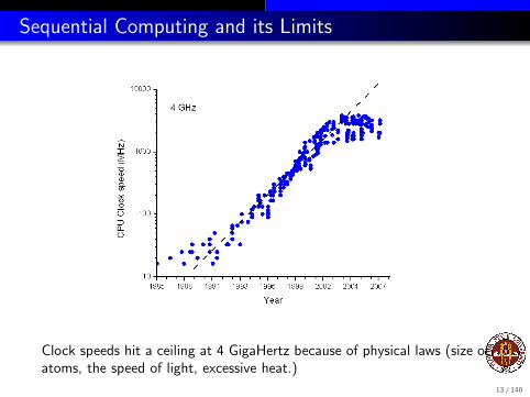
Clock speeds hit a ceiling at 4 GigaHertz because of physical laws (size ofatoms, the speed of light, excessive heat.)

13 / 140


Future processors will have the same clock speed as today...

What do we do for improved performance?

14 / 140


Hardware possibilities include:

several, or many, cores on a processor;

several, or many, processors in one machine;

tens of machines with very fast communication;

hundreds or thousands of machines with moderately fastcommunication.

15 / 140


Software possibilities include:

System software to control multiple cores or processors

Software to allow separate machines to communicate

Compilers that extend common languages to control multipleprocesses

Algorithms chosen to exploit any inherent parallelism in a problem

16 / 140



2 Data Dependence

How many tasks can we do at the same time?

17 / 140

Data Dependence

Tasks are ordered sequentially because a sequential computer can only doone at a time. But is it logically necessary?

18 / 140

Data Dependence

Computational biologist Peter Beerli has a program named MIGRATEwhich infers population genetic parameters from genetic data usingmaximum likelihood by generating and analyzing random genealogies.

His computation involves:

1 an input task

2 thousands of genealogy generation tasks.

3 an averaging and output task

19 / 140

Data Dependence

In an embarrassingly parallel calculation, there’s a tiny amount ofstartup and wrapup, and in between, complete independence.

20 / 140

Data Dependence

A more typical situation occurs in Gauss elimination of a matrix.Essentially, the number of tasks we have to carry out is equal to thenumber of entries of the matrix on the diagonal and below the diagonal.

A diagonal task seeks the largest element on or below the diagonal.

A subdiagonal task adds a multiple of the diagonal row that zeroes outthe subdiagonal entry.

Tasks are ordered by column. For a given column, the diagonal taskcomes first. Then all the subdiagonal tasks are independent.

21 / 140

Data Dependence

In Gauss elimination, the number of independent tasks available variesfrom step to step.

22 / 140

Data Dependence

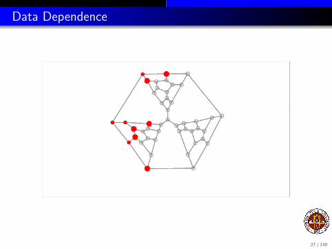
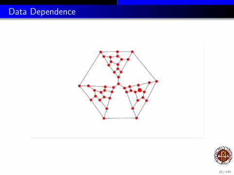
An example that is less structured occurs whenever the computation canbe regarded as “exploring” a graph, that is, starting at one root node andfollowing the edges to visit all the nodes.

If the tasks depend on each other in the same way that the nodes areconnected back to the root node, then the dependence graph is the treethat starts at the root node.

23 / 140

Data Dependence

24 / 140

Data Dependence

25 / 140

Data Dependence

26 / 140

Data Dependence

27 / 140

Data Dependence

28 / 140

Data Dependence

29 / 140

Data Dependence

30 / 140

Data Dependence

31 / 140

Data Dependence

32 / 140

Data Dependence

In our example, we saw the graph, so we know what to expect. In a realproblem, the graph might be much more irregular, and we would neversee it.

If we are working in parallel, and can do P tasks on a step, then at eachstep, we are completing anywhere from 1 to P tasks.

And by completing these tasks, we encounter an unknown number of newtasks that are ready to be worked on.

A sequential program uses a stack to work through such tasks.

33 / 140

Data Dependence - Vocabulary

If the tasks we are considering are relatively large computations, we speakof coarse grained parallelism. Such tasks can often be distributedacross multiple computers, since the amount of communication (whentasks begin and end) will be relatively small compared to the amount ofcomputation done.

If these tasks are on the order of a statement or a block of statements,we speak of fine grained parallelism. Here we presume the tasks will allbe done on one computer, but perhaps by different co-processors whichshare the memory.

34 / 140

Data Dependence

Data dependence between tasks T1 and T2, involving variable V, occursif either:

1 V is an input to one task and an output of the other.

2 V is an output of both tasks

Data dependence means T1 and T2 cannot be performed in parallel.

35 / 140

Data Dependence

If tasks T1 and T2 are sets of computer statements, then dependenceoccurs if one task’s “left hand side” variable V occurs anywhere in theother task (on the left or right hand side).

Arrays, pointers and functions will complicate this test!

36 / 140

Data Dependence

What pairs of tasks can be run in parallel?

a = f + 5 Task 1b = sqrt ( w )

-------------------e = 2 * e + 1 Task 2f = b + d * e

-------------------c = f * f - d Task 3d = min ( d, c )

-------------------a = 1 Task 4c = 2

37 / 140

Data Dependence

For which loops are the iterations data dependent?

for ( i = 1; i < n - 1; i++ ) Loop 1x[i] = x[i] + x[i-1];

-------------------do j = 2, n - 1y(j) = ( y(j) - y(j+1) ) / 2 Loop 2

end do-------------------for k = 2 : n - 1 Loop 3z(k) = z(k) * z(k);

end

38 / 140



2 Data Dependence

3 Parallel Algorithms

We try to understand how parallelism could help us.

39 / 140

Parallel Algorithms

There is a lot we need to understand, but we have to start somewhere!

Let’s consider how certain problems could be treated if some kind ofparallel computing facility was available.

We won’t worry about the details, but we will try to pay attention tosome common themes.

40 / 140

Parallel Algorithms

At the end of the year, a teacher has 1,000 test scores to add up andaverage. Her noisy classroom of 50 kids is distracting her.

She comes up with several ways to use their help.

41 / 140

Parallel Algorithms

Method 1

The students could all come up to the front desk and stare at thegradebook with the 1,000 scores.

Each student could take one row of the table of scores and add it up.

They only have one sheet of paper to work on, so the teacher would markit off into 50 separate boxes for their intermediate sums.

The teacher would pencil in a 0 for the initial sum. Students take turnserasing the current sum, adding their result, and writing the new sum.

42 / 140

Parallel Algorithms

Method 2

The teacher could hand each student one set of grades to add.

Each student work at their desk, without worrying about any interferencefrom others.

As soon as they have computed their sum, they call the teacher over,who adds the result to the total.

43 / 140

Parallel Algorithms

These two simple stories might seem very similar, but they suggest twodifferent ways to go about a parallel algorithm; we will come back tothese ideas soon.

But let us take from this exercise a simple model for a parallelcomputation.

Let’s say there’s a Boss or Master, with N pieces of data, typically X1,X2, ...XN.

We let p stand for the number of helpers or agents, each of whomworks with n pieces of data, typically x1, x2,... xn.

44 / 140

Parallel Algorithms

To sum N numbers, the Master sends n numbers to each agent.

When an agent returns the partial sum, the Master performs the finalreduction of the partial sums to a single total.

The same amount of computation is done, and happens faster becausethe big sum has been broken up.

But this computation may take much longer. For every computation(plus sign) there is also a communication (send the number).Communication between machines takes much longer than computation(100 or 1,000 times longer).

We will see other examples of how communication costs are an importantitem in judging a parallel algorithm.

45 / 140

Parallel Algorithms

Suppose on the other hand that communication costs are insignificant,and that computing power is so cheap that we have one agent for everynumber Xi in our sum.

Suppose that an agent can add two numbers in one time step, and that asequential program would take about N steps to compute the sum.

Then we can add N numbers in log(N) time using our agents.

We start with each agent having one number.

On the first step, each even agent I sends its value to the agent I/2, whoadds it to its number.

The even agents drop out, we renumber the odd agents, and repeat theprocess til we end up with the total sum stored by agent 1.

46 / 140

Parallel Algorithms

The addition examples may seem unrealistic and impractical.

But the pattern of combination used by these simple tasks often occursin more complicated calculations. In those cases, a similar pattern ofdata distribution and combination might turn out to be appropriate andefficient.

47 / 140

Parallel Algorithms

Now suppose we have a set of N numbers to sort.

You probably know several algorithms for sorting, but they are allexpressed sequentially.

Suppose we use N/2 agents, giving each two values, y1 and y2.

We number the agents, and imagine them standing in a line, able tocommunicate with their left and right neighbors.

The following algorithm sorts the data in N steps. The best sequentialalgorithms take about N log(N) steps.

48 / 140

Parallel Algorithms

During a step, each agent:

sorts its two values so that y1 < y2,

sends a copy of y1 left;receives a number x2 from the left.y1 = max ( y1, x2 );

sends a copy of x2 right.receives a number z1 from the right.y2 = min ( y2, z1).

49 / 140

Parallel Algorithms

Some features of this algorithm that occur elsewhere:

the agents are arranged in a communication network

the communication is regular (a number is passed left, then anumber is passed right)

the communication is local (left or right)

If the number of agents is limited, it’s not difficult to modify thealgorithm so that each agent handles more than just 2 values.

By the way, what should we do at the first and last agents?

50 / 140

Parallel Algorithms

Quadrature involves the estimation of the integral of a function over aregion, usually by averaging a number of sample function values.

In the simplest case, the region is a line, the function is “well behaved”,and we know the number of sample values we want.

In that case we can divide the line in segments, and have each agentsample its segment, sum its values and send them to the ”Boss” for afinal total.

51 / 140

Parallel Algorithms

52 / 140

Parallel Algorithms

When a parallel version of an algorithm is produced by subdividing thegeometric region, this technique is known as domain decomposition.

In this case, the division was simple. But sometimes, the subregions willneed to communicate with each other.

If the function changes behavior, then it may be necessary to do moresampling in some regions. Instead of dividing the whole region into 4segments, we could have given each agent a part, but left most of thework unassigned. As an agent finishes a task, it gets more work. This isknown as dynamic scheduling.

53 / 140

Parallel Algorithms

The power method seeks the maximum eigenvalue λ of a matrix A, andits corresponding eigenvector v.

Starting with an initial estimate for v, we essentially do the following:

v_new = A * v;lambda = v_new’ * v;v = v_new / || v_new ||;

Matrix-vector multiplication is easy to do in parallel. We can divide Ainto p groups of rows, or columns, or even into submatrices. Since thematrix doesn’t change, the communication at each step involves sendingpieces of v and v new back and forth.

54 / 140

Parallel Algorithms

55 / 140

Parallel Algorithms

I mentioned the idea of searching a graph or tree. The solution of aSudoku puzzle is an illustration of this concept. As you can see, thepartially-filled in puzzle includes indicators for the digits that are possiblefillers for the empty boxes.

Every digit represents a task, that is, moving to a new node on the treeand taking yet another (educated) guess.

Clearly, a set of agents could profitably explore different possibilities.

Note that in this example, two agents could start out in differentdirections and end up exploring the same node further down the tree.

This is a problem whose “geometry” is very hard to diagram in advance.

56 / 140

Parallel Algorithms

The heat equation is a model of the kinds of partial differential equationsthat must be solved in scientific computations.

Determine the values of H(x , t) over a range t0 <= t <= t1 and spacex0 <= x <= x1, given an initial value H(x , t0), boundary conditions, aheat source function f (x , t), and a partial differential equation

∂H

∂t− k

∂2H

∂x2= f (x , t)

57 / 140

Parallel Algorithms

An approximate solution to this problem can be computed by using a gridof points in space and time. The values are known at the initial time, andat the left and right endpoints. Internally, we can compute a value at thenext time by a kind of average of the current value with its left and rightneighbors.

We can use domain decomposition, as we did for the quadrature problem.However, we now see that we will need to arrange for communicationbetween neighboring agents, since in some cases, the neighbor of a pointbelongs to a different subregion.

58 / 140

Parallel Algorithms

59 / 140



2 Data Dependence


4 Shared Memory Parallel Computing

A shared memory program runs on one computer with multiple cores.

60 / 140

Shared Memory - Multiple Processors

The latest CPU’s are called dual core and quad core, with rapid increasesto 8 and 64 cores to be expected.

The cores share the memory on the chip.

A single program can use all the cores for a computation.

It may be confusing, but we’ll refer to a core as a processor.

61 / 140


If your laptop has a dual core or quad core processor, then you will see aspeedup on many things, simply because the operating system can rundifferent tasks on each core.

When you write a program to run on your laptop, though, it probably willnot automatically benefit from multiple cores.

62 / 140


63 / 140

Shared Memory - Multiple Local Memories

The diagram of the Intel quad core chip includes several layers of memoryassociated with each core.

The full memory of the chip is relatively “far away” from the cores. Thecache contains selected copies of memory data that is expected to beneeded by the core.

Anticipating the core’s memory needs is vital for good performance.(There are some ways in which a programmer can take advantage of this.)

A headache for the operating system: cache coherence, that is, makingsure the original data is not changed by another processor, whichinvalidates the cached copy.

64 / 140

Shared Memory - NUMA Model

It’s easy for cores to share memory on a chip. And each core can reachany memory item in the same time, known as UMA or “Uniform Accessto Memory”.

Until we get 8 or 16 core processors, we can still extend the sharedmemory model, if we are willing to live with NUMA or “Non-UniformAccess to Memory”.

We arrange several multiprocessor chips on a very high speed connection.It will now take longer for a core on one chip to access memory onanother chip, but not too much longer, and the operating system makeseverything look like one big memory space.

65 / 140

Shared Memory - NUMA Model

Chips with four cores share local RAM, and have access to RAM on otherchips.

VT’s SGI ALTIX systems use the NUMA model.

66 / 140

Shared Memory - Implications for Programmers

On a shared memory system, the programmer does not have to worryabout distributing the data. It’s all in one place or at least it looks thatway!

A value updated by one core must get back to shared memory beforeanother core needs it.

Some parallel operations may have parts that only one core at a timeshould do (searching for maximum entry in vector).

Parallelism is limited to the number of cores on a chip (2, 4, 8?), orperhaps the number of cores on a chip multiplied by the number chips ina very fast local network (4, 8, 16, 64, ...?).

67 / 140

Shared Memory - Implications for Programmers

The standard way of using a shared memory system in parallel involvesOpenMP.

OpenMP allows a user to write a program in C/C++ or Fortran, andthen to mark individual loops or special code sections that can beexecuted in parallel.

The user can also indicate that certain variables (especially “temporary”variables) must be treated in a special way to avoid problems duringparallel execution.

The compiler splits the work among the available processors.

This workshop will include an introduction to OpenMP in a separatetalk.

68 / 140

Shared Memory - Data Conflicts

Here is one example of the problems that can occur when working inshared memory.

Data conflicts occur when data access by one process interferes withthat of another.

Data conflicts are also called data races or memory contention. In part,these problems occur because there may be several copies of a singledata item.

If we allow the “master” value of this data to change, the old copies areout of date, or stale data.

69 / 140

Shared Memory - Data Conflicts

A mild problem occurs when many processes want to read the same itemat the same time. This might cause a slight delay.

A bigger problem occurs when many processes want to write or modifythe same item. This can happen when computing the sum of a vector,for instance. But it’s not hard to tell the processes to cooperate here.

A serious problem occurs when a process does not realize that a datavalue has been changed, and therefore makes an incorrect computation.

70 / 140

Data Conflicts: The VECTOR MAX Code

program main

i n t e g e r i , ndouble p r e c i s i o n x (1000) , x max

n = 1000

do i = 1 , nx ( i ) = rand ( )

end do

x max = −1000.0

do i = 1 , ni f ( x max < x ( i ) ) then

x max = x ( i )end i f

end do

stopend

71 / 140

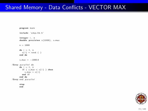
Shared Memory - Data Conflicts - VECTOR MAX

program main

i n c l u d e ’ omp l i b . h ’

i n t e g e r i , ndouble p r e c i s i o n x (1000) , x max

n = 1000

do i = 1 , nx ( i ) = rand ( )

end do

x max = −1000.0

! $omp p a r a l l e l dodo i = 1 , n

i f ( x max < x ( i ) ) thenx max = x ( i )

end i fend do

! $omp end p a r a l l e l

stopend

72 / 140


It’s hard to believe, but the parallel version of the code is incorrect. Inthis version of an OpenMP program, the variable X MAX is shared, thatis, every process has access to it.

Each process will be checking some entries of X independently.

Suppose process P0 is checking entries 1 to 50, and process P1 ischecking entries 51 to 100.

Suppose X(10) is 2, and X(60) is 10000, and all other entries are 1.

73 / 140


Since the two processes are working simultaneously, the following is apossible history of the computation:

1 X MAX is currently 1.

2 P1 notes that X MAX (=1) is less than X(60) (=10,000).

3 P0 notes that X MAX (=1) is less than X(10) (=2).

4 P1 updates X MAX (=1) to 10,000.

5 P0 updates X MAX (=10,000) to 2.

and of course, the final result X MAX=2 will be wrong!

74 / 140


This simple example has a simple correction, but we’ll wait until theOpenMP lecture to go into that.

The reason for looking at this problem now is to illustrate the job of theprogrammer in a shared memory system.

The programmer must notice points in the program where the processorscould interfere with each other.

The programmer must coordinate calculations to avoid such interference.

75 / 140



2 Data Dependence



5 Distributed Memory Parallel Computing

Distributed memory programs run on multiple computers; messages areused to send data and results.

76 / 140

Distributed Memory - Multiple Processors

77 / 140

Distributed Memory

A distributed memory computation manages the resources of severalindependent computers which are joined on a communication network.

Thus, theoretically, no fancy new hardware is needed: just cables and arouter.

If the communication is fast enough, the result is a powerful computingdevice.

78 / 140

Distributed Memory

A distributed memory system will need some kind of software daemon,running on each machine, which will:

copy the program and data files to all machines;

start the program on all the machines;

send and receive messages from programs, holding them til received;

gather program outputs to a single file

shut down programs at the end and clean up

79 / 140

Distributed Memory

A distributed memory system must offer a library that allows a userprogram to make function calls:

to “check in”

to find out how many other processes are running

to request an ID

to send a message to another process

to receive messages from other processes

to request that other processes wait

to “check out”

80 / 140

Distributed Memory

The programmer writes a single program to run on all machines.

This program

defines and initializes data

determines the portion of work that a process will do

shares data with other processes as needed

collects results in the end.

81 / 140

Distributed Memory

How can copies of the same program execute differently on differentmachines?

Each process is assigned a unique ID, which it can find out through afunction call.

Each process can also find out P, the total number of processesparticipating in the calculation.

ID’s run from 0 to P-1. Simply assigning an ID is enough to guide theprocesses to the work they must do.

82 / 140

Distributed Memory

A simple design for parallel programs is the master/worker model.

Process 0 is assigned to control the computation: read input, assignwork, gather results, print reports.

Independent tasks are divided up among processes 1 through P-1.

People like this model because it is not so different from sequentialprogramming - someone is still “in charge”.

IF/ELSE statements separate the master and worker portions of theprogram.

83 / 140

Distributed Memory

Sketch of a master/worker quadrature program:

if ( master )send N to all workersfor each worker I, send A[I], B[I]set Q = 0for each worker I, receive Q_PART[I], add to Q.print "Integral = " Q

elsereceive N from masterreceive A, B from masterQ_PART = 0for N equally spaced X between A and B,Q_PART = Q_PART + F(X)

send Q_PART to master

84 / 140

Distributed Memory

Another design for parallel programs comes from domain decomposition.

If the problem to be solved is associated with a geometric region, thenprocess I is assigned to work in subregion I.

Communication between processes corresponds to the geometry of thesubregions. For the 1D heat equation, each process (except the first andlast) has a left and right neighbor.

Typically, a process must inform its neighbors of data it has updated thatlies on their common boundary.

The amount of communication is typically related to the “area” of theboundary. It’s useful to keep the subregions compact.

85 / 140

Distributed Memory

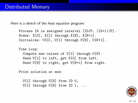
Here is a sketch of the heat equation program:

Process ID is assigned interval [ID/P, (ID+1)/P].Nodes: X[0], X[1] through X[N], X[N+1].Initialize: U[0], U[1] through U[N], U[N+1].

Time Loop:Compute new values of U[1] through U[N].Send U[1] to left, get U[0] from left.Send U[N] to right, get U[N+1] from right.

Print solution at end:

U[1] through U[N] from ID 0,U[1] through U[N] from ID 1, ...

86 / 140

Distributed Memory

Using distributed memory brings some new costs and potential errors.

The costs may include a substantial effort to rethink and rewrite theprogram.

There is also a communication cost that offsets the; remember wesuggested that sending a number somewhere else might take 100 or 1000times as long as performing a computation on that number.

But there are also several new problems that can occur because of thefact that we are trying to communicate between machines.

87 / 140

Distributed Memory

Generally, the processes are free to run independently on the variousmachines, as fast as they can.

In most programs there will be certain synchronization points, that is,lines of code which some or all of the processors must reach at the sametime.

Processors reaching the synchronization point early must wait for theothers.

As an example, if the processors are working together on an iteration,then generally they all must synchronize at the end of each step, to shareupdated information.

88 / 140

Distributed Memory

Synchronization can increase the costs and delays associated withcommunication.

In particular, if the work is poorly divided, or if communication to aparticular processor is slow, or if that processor is less powerful, then it islikely that all the other processors will have to wait at synchronizationpoints.

Problems of this sort are called load balancing problems.

89 / 140

Distributed Memory

Another instance that can involve synchronization involves the sending ofmessages.

In the typical case, only two processes are involved, a sender and areceiver.

In the simplest case, the sender pauses at the SEND statement, thereceiver pauses at the RECEIVE statement. When they are both there,the sender sends the message, the receiver receives it, and sends back aconfirmation.

The idle time that one process spent waiting for the other (asynchronization point) is wasted.

90 / 140

Distributed Memory

There are alternatives when transmitting messages:

1 Synchronous transmission: the message is not transmitted until bothsender and receiver are ready;

2 Buffered transmission: the message is put into a buffer as soon asthe sender is ready. The sender proceeds, and the receiver picks upthe message when it is ready

3 Nonblocking transmission: the receiver indicates that it is ready toreceive the message, but may continue to do other work whilewaiting

91 / 140

Distributed Memory

Not only can message transmission cause delays - it can also cause theprogram to fail entirely.

It is possible to write a program which uses the communication channelsincorrectly, so that messages can’t get through.

Deadlock is a situation in which a process cannot proceed, because it iswaiting for a condition that will never come true.

Recall that in the simplest version of message transmission, a sendercan’t proceed until the message is received; a receiver can’t proceed untilthe message is sent.

92 / 140

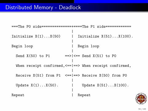
Distributed Memory - Deadlock

Here is a recipe for deadlock, using our heat equation problem.

Suppose we use 2 processes, each responsible for computing 50 values ofX. To keep things simple, we will refer to all 100 values of X as thoughthey were in a single global array.

Process P0 has X(1) through X(50)process P1 has X(51) through X(100).

P0 needs updated copies of X(51) from P1;P1 needs updated copies of X(50) from P0.

If they do this in the wrong way, they deadlock.

93 / 140

Distributed Memory - Deadlock

===The P0 side==============+====The P1 side============|

Initialize X(1)...X(50) | Initialize X(51)...X(100).|

Begin loop | Begin loop|

Send X(50) to P1 ==>|<== Send X(51) to P0|

When receipt confirmed,<==|==> When receipt confirmed,|

Receive X(51) from P1 <==|==> Receive X(50) from P0|

Update X(1)...X(50). | Update X(51)...X(100).|

Repeat | Repeat

94 / 140

Distributed Memory - Programmer Implications

MPI is a system designed for parallel programming on distributedmemory systems.

MPI allows the user to write a program, in C/C++ or Fortran.

The user program calls various functions from the MPI library in order todetermine the process ID, send messages, and other tasks.

Depending on the installation, the user runs a job interactively, using acommand like mpirun or through a batch system, which requires a jobscript.

The next two days of this workshop will concentrate on a detailedpresentation of MPI.

Let’s get a preview of an MPI program.

95 / 140

Distributed Memory: The VECTOR MAX Code

program main

i n c l u d e ’ mpi f . h ’

i n t e g e r i di n t e g e r i e r ri n t e g e r p

c a l l MPI I n i t ( i e r r )c a l l MPI Comm rank ( MPI COMM WORLD, id , i e r r )c a l l MPI Comm size ( MPI COMM WORLD, p , i e r r )

c a l l d o s t u f f ( id , p )

c a l l MPI F i n a l i z e ( i e r r )

stopend

96 / 140


s u b r o u t i n e d o s t u f f ( id , p )

i n c l u d e ’ mpi f . h ’

i n t e g e r i , id , i e r r , j , p , s r c , tag , t a r g e tdouble p r e c i s i o n x (1000) , x max , x max l o c a l

i f ( i d == 0 ) then <−−MASTER c r e a t e s data and sends i t

do i = 1 , p − 1

do j = 1 , 1000x ( j ) = rand ( )

end do

t a r g e t = itag = 1c a l l MPI Send ( x , 1000 , MPI DOUBLE PRECISION , t a r g e t , tag ,

& MPI COMM WORLD, i e r r )

end do

e l s e <−− WORKERS r e c e i v e data

s r c = 0tag = 1c a l l MPI Recv ( x , 1000 , MPI DOUBLE PRECISION , s r c , tag ,

& MPI COMM WORLD, s t a t u s , i e r r )

end i f

97 / 140


i f ( i d == 0 ) then <−− MASTER r e c e i v e s maximums .

x max = −1000.0tag = 2

do i = 1 , p − 1

c a l l MPI Recv ( x max l o ca l , 1 , MPI DOUBLE PRECISION ,& MPI ANY SOURCE , tag , MPI COMM WORLD, s t a t u s , i e r r )

x max = max ( x max , x max l o c a l )

end do

e l s e <−− WORKERS send maximums .

x max l o c a l = x (1 )

do i = 2 , ni f ( x max l o c a l . l t . x ( i ) ) x max l o c a l = x ( i )

end do

t a r g e t = 0tag = 2c a l l MPI Send ( x max l o ca l , 1 , MPI DOUBLE PRECISION , t a r g e t ,

& tag , MPI COMM WORLD, i e r r )

end i f

r e t u r nend

98 / 140



2 Data Dependence




6 Performance Measurements for Parallel Computing

What does faster mean? Can you have too many parallel processes?

99 / 140

Performance Measurement

Performance measurements allow us to estimate whether our program isrunning at maximum speed on a given computer.

They can help us to estimate the running time required if we double theproblem size N.

They can help us compare algorithms, compilers, computers.

We can try to understand how the problem size N and the number ofparallel processes P interact, so that we can find the “sweet spot”, therange of parameters that yield good performance.

100 / 140


A common performance measurement is the MegaFLOPS rate.

This measurement concentrates entirely on the speed with which a givenset of floating-point arithmetic operations is carried out.

A FLOP is a floating point operation: addition or multiplication.

We can sometimes estimate the FLOPs required for a calcuation.

Matrix multiplication takes 2N2,typical Gauss elimination requires about 2

3N3.

101 / 140

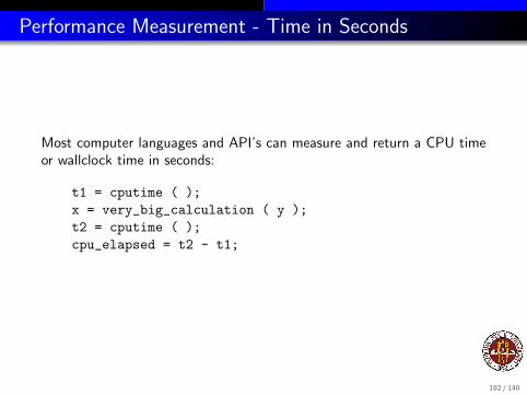
Performance Measurement - Time in Seconds

Most computer languages and API’s can measure and return a CPU timeor wallclock time in seconds:

t1 = cputime ( );x = very_big_calculation ( y );t2 = cputime ( );cpu_elapsed = t2 - t1;

102 / 140


To keep things from getting too big, we typically scale the FLOPS by amillion.

Now if we divide the work, in MegaFLOPs, by the elapsed CPU time, inseconds, we get the MegaFLOPS rate:

MFLOPS = ( FLOPS / 1,000,000 ) / seconds

103 / 140


A MegaFLOPS rate is a reasonable number to use when comparingprograms or computers.

Even on a sequential (non-parallel) computation, there can be variationsin the computed rate. It’s important to run a “big enough” program for a“long enough” time so that the rate settles down.

A MegaFLOPS rate is at the heart of the LINPACK benchmarkprogram, which measures the speed at which a 1000x1000 linear systemis solved.

104 / 140

Performance Measurement - The LINPACK Benchmark

Table: Sample LINPACK Ratings

Rating Computer Language Comment108 Apple G5 C used ”rolled” loops184 Apple G5 C used ”unrolled” loops221 Apple G5 F77 gfortran compiler227 Apple G5 Java

20 Apple G5 MATLAB using ”verbatim” LINPACK1857 Apple G5 MATLAB using MATLAB “backslash”

105 / 140


Rating Computer Site Processors12,250,000 2.3 GHz Apple VT, System X 2,20013,380,000 Xeon 53xx “Bank in Germany” 2,64042,390,000 PowerEdge Maui 5,200

102,200,000 Cray XT3 “Red Storm”, Sandia 26,569126,900,000 SGI Altix New Mexico 14,336167,300,000 BlueGeneP FZ Juelich 65,536478,200,000 BlueGeneL DOE/NNSA/LLNL 212,992

1,026,000,000 Cell+Opteron Roadrunner, LANL 12,240+6,562

1000 MegaFLOPS = 1 GigaFLOPS

1000 GigaFLOPS = 1 TeraFLOPS

1000 TeraFLOPS = 1 PetaFLOPS(30 May 2008)

106 / 140


Even if you only have your own computer to experiment with, theLINPACK benchmark can sometimes give you some insight into whatgoes on inside.

Run the program for a series of values of N. We often see three phases ofbehavior:

a rising zone: cache memory and processor are not challenged.

a flat zone, the processor is performing at top efficiency.

a decaying zone, the matrix is so large the cache can’t hold enoughdata to keep the processor running at top speed.

107 / 140


108 / 140


CPU time is the right thing to measure for sequential computing,

Typical runs occur on a time-shared computer.Your main cost is the arithmetic calculations.

C/C++:

ctime = ( double ) clock ( )/ ( double ) CLOCKS_PER_SEC;

FORTRAN90:

call cpu_time ( ctime )

109 / 140


Wallclock time is what you measure for parallel programming.

A typical run is on a dedicated set of processors.Cost is number of processors times the elapsed time.

OpenMP (C/C++/FORTRAN):

wtime = omp_get_wtime ( );

MPI (C/C++/FORTRAN):

wtime = MPI_Wtime ( );

110 / 140

Performance Measurement - Wallclock Time

Wallclock time forces us to count communication, memory access, andother noncomputational costs.

The total CPU time of a parallel computation is usually significantlyhigher than for a sequential computation.

We assume (correctly) that individual processors are cheap;our concern is to cut the real time required for an answer.

We can still compute MegaFLOPS ratings, but our timings will be interms of wall clock time!

111 / 140

Performance Measurement - Problem Size

Problem size, symbolized by N, affects our performance ratings.Very small and very large problems will do badly, of course.What happens for “reasonable” values of N?

Fix the number of processors P, and record the solution time T for arange of N values.

For the Fast Fourier Transform, we know the algorithm, so we know thenumber of FLOPS, and can compute a MegaFLOPS rate.

If we are using the machine well, it should be able to work at roughly aconstant rate for a wide range of N.

112 / 140

MFLOPS Plot for FFT + OpenMP on 2 Processors

113 / 140


The story is incomplete though! Let’s go back (like I said you should do!)and gather the same data for 1 processor.

It’s useful to ask ourselves, before we see the plot, what we expect orhope to see. Certainly, we’d like evidence that the parallel code wasfaster.

But what about the range of values of N for which this is true?

Here we will see an example of a “crossover” point. For some values ofN, running on one processor gives us a better computational rate (and afaster execution time!)

114 / 140

MFLOPS Plot for FFT + OpenMP on 1 versus 2Processors

115 / 140


Now, roughly speaking, we can describe the behavior of this FFTalgorithm, (at least on 2 processors) as having three ranges, and I willinclude another which we do not see yet:

startup phase, of very slow performance;

surge phase, in which performance rate increases linearly;

plateau phase, in which performance levels off;

saturation phase, in which performance deteriorates;

116 / 140


It should become clear that a parallel program may be better than asequential program...eventually or over a range of problem sizes or whenthe number of processors is large enough.

Just from this examination of problem size as an influence onperformance, we can see evidence that parallel programming comes witha startup cost. This cost may be excessive for small problem size ornumber of processors.

117 / 140


While a MegaFLOPS rate can be very illuminating, it’s only computableif the FLOPs can be determined.

That assumes the entire computation is basically one simple algorithm(Gauss elimination, FFT, etc).

This is NOT true for most scientific programs of interest.

Program run time is very accessible. We can learn by studying itsdependence on the number of processors, and on the problem size.

118 / 140

Performance Measurement - Speedup

Speedup measures the work rate as we add processors.

The work W depends on the problem size N.

For a fixed N, we solve the problem for an increasing series of processorsP, and record the time T.

For a “perfect speedup”, we would hope that

T = W /P

Doubling the processors would halve the time, and we could drive T tozero if we had enough processors.

119 / 140

Performance Measurement - Speedup

To define a formula for speedup S, we time the problem solution using 1processor, and set that to be T(1).

Then if we repeat the computation using P processors, the speedupfunction is defined as

S(P) = T (1)/T (P)

In a perfect world, S(P) would equal P.Tracking S(P) indicates how well our program parallelizes.

120 / 140

Performance Measurement - Number of Processors

When we plot the speedup function P versus S(P), the first data pointshould be (1,1). This simply means that we are normalizing the data sothat the computational rate on one processor is set to 1.

When we run the program on two processors, our time probably won’t behalf of T(1), but maybe it will be 0.55 times it. We plot the point (2,1/0.55) = (2, 1.818).

The ideal speedup behavior is a diagonal line, but we will see the actualbehavior is a curve that “strives” for the diagonal line at first, and then“gets tired” and flattens out (and will actually decrease if we go out toofar!)

121 / 140

Performance Data for a version of BLAST

122 / 140


When you plot data this way, there is a nice interpretation of the scale.In particular, note that when we use 6 processors, our speedup is about4.5. This means that we when use 6 processors, the program speeds upas though we had 4.5 processors (assuming a perfect speedup).

Some people define the parallel effficiency as the ratio of the effectivenumber of processors divided by the actual number. For this case, at 6processors our efficiency would be 0.75. (It’s actually the slope of thespeedup graph).

You can also see the curve flattening out as the number of processorsincreases.

123 / 140


The speedup function really depends on the problem size as well as thenumber of processors, so we could write S(P,N).

If we fix P, and consider a sequence of increasing sizes N, we often seethe familiar rise, plateau and deterioration behavior.

But it is often the case that the plateau, the range of problem sizes withgood performance, moves and widens as we increase P.

For a fixed P, bigger problems run better.For a fixed N, adding processors reduces time, but also efficiency.

124 / 140


We can try to display the relationship between P and N on one plot.

The problem size for the BLAST program is measured in the length ofthe protein sequence being analyzed, so we can’t pick N arbitrarily.

Let’s go back and do timings for sequences of 5 different sizes, anddisplay a series of S(P) curves for different N.

125 / 140

Performance Data for a version of BLAST

126 / 140

Performance Measurement - Applying for Computer Time

To get time on a parallel clusters, you must justify your request withperformance data.

You should prepare speedup plots for a few typical problem sizes N andprocessors from 1, 2, 4, 8, ... to P.

If you still get about 30% speedup using P processors, your request isreasonable.

In other words, if a 100 processor machine would let you run 30 timesfaster, you’re got a good case.

127 / 140



2 Data Dependence




6 Performance Measurements for Parallel Computing

7 Auto-Parallelization

A quick and easy way to try parallel programming on your code.

128 / 140

Auto-Parallelization

Auto-parallelization is a feature, available with some compilers, whichattempts to identify portions of the source code which can be executed inparallel.

This is an easy way to experiment with the potential for parallelexecution.

This feature is generally only available for use on shared memorymachines - which includes laptops with dual cores, the Virginia Tech SGIsystems.

The executable code must be run in the appropriate parallel environment(that is, you must set the OpenMP environment variable that specifiesthe number of threads to use).

129 / 140


Auto-parallelization is cautious: its goal is only to make changes that itcan guarantee will execute the same on multiple processors.

Auto-parallelization is limited: it will miss some chances to parallelize.

Auto-parallelization is not perfect: it may be fooled into parallelizingsome code when it is not safe to do so.

So code that is auto-parallelized should be checked for accuracy as wellas timed for speedup.

130 / 140

Auto-Parallelization - GCC Compiler Flags

GCC/G++/GFORTRAN compilers:

gcc -ftree-vectorize -O2 myprog.c

Add the switch -maltivec on PowerPC hardware.

Note that -ftree-vectorize is one word!

These commands invoke auto-vectorization, which is less ambitious.GCC is currently developing auto-parallelization features, but they are notwidely used yet.

131 / 140

Auto-Parallelization - IBM Compiler Flags

IBM FORTRAN compiler:

xlf_r -O3 -qsmp=auto -qreport=smplist myprog.f

IBM C compiler:

xlc_r -O3 -qsmp=auto -qreport=smplist myprog.c

The optional -qreport=smplist switch reports on why some loops couldnot be parallelized.

There is also a -qsource switch which produces a compiler listing.

132 / 140

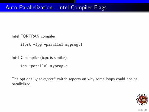
Auto-Parallelization - Intel Compiler Flags

Intel FORTRAN compiler:

ifort -fpp -parallel myprog.f

Intel C compiler (icpc is similar):

icc -parallel myprog.c

The optional -par report3 switch reports on why some loops could not beparallelized.

133 / 140

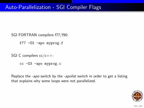
Auto-Parallelization - SGI Compiler Flags

SGI FORTRAN compilers f77/f90:

f77 -O3 -apo myprog.f

SGI C compilers cc/c++:

cc -O3 -apo myprog.c

Replace the -apo switch by the -apolist switch in order to get a listingthat explains why some loops were not parallelized.

134 / 140

Auto-Parallelization - Sun Compiler Flags

Sun FORTRAN compilers f77/f90/f95:

f77 -fast -autopar -parallel -loopinfo myprog.f

Sun C compilers:

cc -xautopar -xparallel -xloopinfo myprog.c

The optional loopinfo switch reports on why some loops could not beparallelized.

135 / 140

Auto-Parallelization - Execution

To run the program, first set the OpenMP environment variable toindicate how many threads you want (perhaps 2 or 4):

Bourne, Korn and Bash shell users:

export OMP_NUM_THREADS=4

C and T shell users:

setenv OMP_NUM_THREADS 4

Then run your program with the usual ./a.out command.

136 / 140

Auto-Parallelization - Obstacles to good results

loops that contain output statements

exiting a loop early

while loops

loops that call functions

loops with very little work

loops with low iteration count - N is small

loops that compute scalar functions of vector data: maximum, dotproduct, norm, integral estimates

loops with complicated array indexing - possible data dependence

loops with actual data dependence

137 / 140


The code produced by the auto-parallelizer may run more slowly, or evenincorrectly.

However, it can be a very useful place from which to begin parallelizationefforts.

Some compilers offer a listing that shows why some loops were notparallelized. Working from this listing, it may be possible to modify loopsso that the auto-parallelizer can handle them.

Moreover, the auto-parallizer may even produce a revised version of thesource code, including parallelization directives. This code may be veryuseful as a starting point for further parallelization “by hand.”

138 / 140

Conclusion - Don’t Panic!

A simple model of the two kinds of parallel programming:

shared memory, more than one processor can see the problem andhelp out; sometimes processors can get in the way of each other

distributed memory, the problem is divided up in some way;processors work on their part in isolation, and send messages tocommunicate

In the next few days, we’ll implement these ideas to make practicalparallel programs.

139 / 140

Conclusion - Don’t Panic

140 / 140

Date post:	18-Feb-2022
Category:	Documents
Upload:	others
View:	12 times
Download:	0 times

Parallel Programming Concepts

Documents