Parallel simulation of reinforced concrete sructures using ...

University of New MexicoUNM Digital Repository

Civil Engineering ETDs Engineering ETDs

7-1-2011

Parallel simulation of reinforced concrete sructuresusing peridynamicsNavid Sakhavand

Follow this and additional works at: https://digitalrepository.unm.edu/ce_etds

This Thesis is brought to you for free and open access by the Engineering ETDs at UNM Digital Repository. It has been accepted for inclusion in CivilEngineering ETDs by an authorized administrator of UNM Digital Repository. For more information, please contact [email protected].

Recommended CitationSakhavand, Navid. "Parallel simulation of reinforced concrete sructures using peridynamics." (2011).https://digitalrepository.unm.edu/ce_etds/42

https://digitalrepository.unm.edu?utm_source=digitalrepository.unm.edu%2Fce_etds%2F42&utm_medium=PDF&utm_campaign=PDFCoverPages

https://digitalrepository.unm.edu/ce_etds?utm_source=digitalrepository.unm.edu%2Fce_etds%2F42&utm_medium=PDF&utm_campaign=PDFCoverPages

https://digitalrepository.unm.edu/eng_etds?utm_source=digitalrepository.unm.edu%2Fce_etds%2F42&utm_medium=PDF&utm_campaign=PDFCoverPages

https://digitalrepository.unm.edu/ce_etds?utm_source=digitalrepository.unm.edu%2Fce_etds%2F42&utm_medium=PDF&utm_campaign=PDFCoverPages

https://digitalrepository.unm.edu/ce_etds/42?utm_source=digitalrepository.unm.edu%2Fce_etds%2F42&utm_medium=PDF&utm_campaign=PDFCoverPages

mailto:[email protected]

Navid SakhavandCandidate

Civil EngineeringDepartment

This thesis is approved, and it is acceptable in qualityand form for publication:

Approved by the Thesis Committee:

~G.w1l*~y::~~:4-~

7?

PARALLEL SIMULATION OF REINFORCED CONCRETE

STRUCTURES USING PERIDYNAMICS

by Navid Sakhavand B.S. Civil Engineering, Sharif University of Technology, 2008 THESIS Submitted in Partial Fulfillment of the Requirements for the Degree of Master of Science Civil Engineering The University of New Mexico Albuquerque, New Mexico May, 2011

iii

© 2011, Navid Sakhavand

iv

DEDICATION

To my Beloved Mom who loves me, like nobody

To my Dear Dad who supports me, like nobody

To my sisters, Nooshin and Nahal

v

ACKNOWLEDGEMENTS

I owe my utmost gratitude to Prof. Walter Gerstle, my advisor, for his patience,

support, guidance and understanding during the time of my research.

I am heartily thankful to my co-advisor, Prof. Susan Atlas, whose encouragement,

supervision and support enabled me to develop an understanding of the subject.

It is a pleasure to thank Dr. Stewart Silling whose kind concern and consideration

regarding my research and my academic achievements is acknowledged.

I would also like to express gratitude to Prof. Timothy Ross and Prof. Percy Ng,

members of my committee, for their comments and suggestions.

Also, I thank the Center for Advanced Research Computing for the use of

facilities and help in harnessing the supercomputers.

Lastly, I offer my regards and blessings to my family, my friends, and all of those

who supported me in any respect during the completion of my thesis.



by Navid Sakhavand B.S. Civil Engineering, Sharif University of Technology, 2008 ABSTRACT OF THESIS Submitted in Partial Fulfillment of the Requirements for the Degree of Master of Science Civil Engineering The University of New Mexico Albuquerque, New Mexico May, 2011

vii



by

Navid Sakhavand

B.S., Civil Engineering, Sharif University of Technology, 2008

M.S., Civil Engineering, University of New Mexico, 2011

ABSTRACT

The failure of concrete structures involves many complex mechanisms.

Traditional theoretical models are limited to specific problems and are not applicable to

many real-life problems. Consequently, design specifications mostly rely on empirical

equations derived from laboratory tests at the component level. It is desirable to develop

new analysis methods, capable of harnessing material-level test parameters.

To overcome limitations and shortcomings of models based on continuum

mechanics and fracture mechanics, Stewart Silling introduced the concept of

peridynamics in 1998. Similar to molecular dynamics, peridynamic modeling of a

physical structure involves simulating interacting particles subjected to an empirical

viii

“force field”. The evolution of interacting particles determines the deformation of the

structure at a given time due to the applied boundary condition.

As a particle-based model, peridynamics requires the repeated evaluation of many

particle interactions which is computationally demanding. However, with today’s

inexpensive computing hardware, parallel algorithms can be utilized to run such

problems on multi-node supercomputers with fast interconnects. However, existing codes

tend to be domain-specific with too many built-in physical assumptions.

In this work, a novel method for parallelization of any particle-based simulation is

presented which is quite general and suitable for simulating diverse physical structures. A

scalable parallel code for molecular dynamics and peridynamics simulation, PDQ, is

described which implements a novel wall method parallelization algorithm, developed as

part of this thesis. PDQ partitions the geometric domain of a problem across multi-nodes

while the physics is left open to the user to decide whether to simulate a solvated protein

or alloy grain boundary at the atomic scale or to simulate cracking phenomena in

concrete via peridynamics. A further extension of PDQ brings more flexibility by

allowing the user to define any desired number of degrees of freedom for each particle in

a peridynamics simulation.

At the end of this thesis, plain, reinforced and prestressed concrete benchmark

problems are simulated using PDQ and the results are compared to available design code

equations or analytical solutions.

This research is a step toward next level of computational modeling of reinforced

concrete structures and the revolutionizing of how concrete is analyzed and also how

concrete structures are designed.

ix

TABLE OF CONTENTS

LIST OF FIGURES ........................................................................................... xiii

1. INTRODUCTION ...................................................................................... 1

1.1. Motivation ............................................................................................. 1

1.2. Background ............................................................................................ 4

1.2.1. Peridynamics ...................................................................................... 4

1.2.2. Molecular dynamics ........................................................................... 5

1.2.3. Scalable parallel computing ............................................................... 6

1.3. Objectives of thesis ................................................................................ 7

1.4. Scope of thesis ....................................................................................... 9

2. LITERATURE REVIEW ........................................................................ 11

2.1. Peridynamics ....................................................................................... 11

2.1.1. Micropolar peridynamic modeling ................................................... 13

2.1.2. Peridynamic states ............................................................................ 15

2.1.3. Implementation of peridynamics within finite element framework . 18

2.1.4. Multi-physical peridynamics ............................................................ 19

2.2. Computational algorithms for parallel simulations ............................. 22

2.2.1. The neighbor list method .................................................................. 24

2.2.2. The multi-cell method ...................................................................... 25

x

2.2.3. The midpoint method ....................................................................... 27

2.2.4. Plimpton’s method of processor communication ............................. 29

2.2.5. Zonal methods .................................................................................. 31

2.3. Existing parallel codes for MD and PD ............................................... 31

2.3.1. SPaSM .............................................................................................. 32

2.3.2. LAMMPS ......................................................................................... 33

2.3.3. GROMACS ...................................................................................... 34

2.3.4. Desmond ........................................................................................... 34

2.3.5. NAMD .............................................................................................. 35

2.3.6. EMU ................................................................................................. 35

2.4. Summary .............................................................................................. 36

3. IMPLEMENTATION OF WALL METHOD IN PDQ ........................ 38

3.1. Mapping between procCubes and processors (processor layout) ... 39

3.1.1. Identification of adjacent processors ................................................ 42

3.1.2. Periodic boundary conditions (PBC) ................................................ 43

3.2. Identification and mapping of cells (cell layout) ................................. 45

3.3. Particle allocation to processors .......................................................... 46

3.4. Particle allocation to cells (Linked List and Head arrays) .......... 48

3.5. Interaction paths .................................................................................. 50

xi

3.6. Particle communication ....................................................................... 55

3.7. Particle interaction ............................................................................... 60

3.8. Message components (beams, columns, and cornices) ....................... 61

3.9. Force communication .......................................................................... 63

3.10. Integration ............................................................................................ 63

3.11. Particle shuffling .................................................................................. 64

3.12. Generalization of degrees of freedom ................................................. 64

3.13. Summary .............................................................................................. 65

4. EXAMPLE PROBLEMS ......................................................................... 67

4.1. Plain concrete cantilever beam ............................................................ 70

4.2. Reinforced concrete cantilever beam .................................................. 74

4.3. Simply supported plain concrete beam ................................................ 79

4.4. Simply supported reinforced concrete beam ....................................... 81

4.5. Lap splice pullout ................................................................................ 85

4.6. Prestressed concrete beam ................................................................... 91

4.7. Scalability and timing performance ..................................................... 96

5. CONCLUSIONS ....................................................................................... 99

5.1. Summary and conclusions ................................................................... 99

5.2. Future work ........................................................................................ 100

APPENDIX ........................................................................................................ 103

xii

REFERENCES………..........………………………………………………….122

xiii

LIST OF FIGURES

Figure 1.1 – Shear failure of a prestressed concrete beam, from [Runzell et al. 2008] ...... 1

Figure 1.2 - Damaged column at Olive View Hospital, from [Steinbrugge 1992] ............. 2

Figure 1.3 – 2D cantilever beam subjected to uniform downward loading ........................ 7

Figure 2.1 – Terminology for peridynamic model ............................................................ 12

Figure 2.2 - Terminology for micropolar peridynamic model (from [Gerstle, Sau and

Silling 2005]) ........................................................................................................ 14

Figure 2.3 - Micropolar constitutive model for concrete (from [Gerstle et al. 2007b]) ... 17

Figure 2.4 - Shear beam at ultimate stage (from [Gerstle, Sau and Aguilera 2007]) ....... 18

Figure 2.5 – Example of finite element implementation of peridynamic method (from

[Gerstle, Sau and Silling 2007]) ............................................................................ 19

Figure 2.6 - Interaction path in multi-cell method in 2D, The gray colored cell interacts

with adjacent cells following the path shown [Beazley and Lomdahl 1992], In this

example, each node of the parallel machine has a single processor only ............. 26

Figure 2.7 - Particles distributed in 3x3 processors [Bowers et al. 2006] ........................ 28

Figure 2.8 - Plimpton’s method of message passing [Plimpton 1993] ............................. 30

Figure 3.1 - Global physical domain subdivided into 2 x 3x3 = 18 procCubes ........... 39

Figure 3.2 - Processors and associated procCubes. Processors 6, 7, and 8 are connected

to their associated procCubes as examples ....................................................... 41

Figure 3.3 - Interchangeable coordinate systems .............................................................. 43

Figure 3.4 - Periodic boundary condition in 2D ............................................................... 44

xiv

Figure 3.5 – A procCube and its cells. Cells are indexed from 1 to 60 in the 1D

coordinate system .................................................................................................. 46

Figure 3.6 - Cells 1 and 2, Linked List and Head Arrays (Adapted from [Allen and

Tildesley 1987]) .................................................................................................... 49

Figure 3.7 - Cells and their interaction paths .................................................................... 50

Figure 3.8 – An example procCube and its walls, (a) cells IDs of the North and the

South walls local to the procCube domain mapped to the wall domain ........... 52

Figure 3.9 - Message passing five steps ............................................................................ 57

Figure 3.10 – Third step of receiving adjacent walls, necessary columns from southeast

and southwest procCubes shown in yellow ...................................................... 59

Figure 3.11 – Walls, beams, columns and cornices are components of the messages ..... 62

Figure 4.1 – Peridynamic constitutive model for concrete ............................................... 68

Figure 4.2 – Peridynamic constitutive model for steel ..................................................... 69

Figure 4.3 – Description of cantilever plain concrete beam ............................................. 71

Figure 4.4 – Applied force vs. time .................................................................................. 72

Figure 4.5 – Deformed shape of cantilever plain concrete beam using PDQ .................... 73

Figure 4.6 – Displacement vs. force plot .......................................................................... 74

Figure 4.7 – Description of cantilever reinforced concrete beam ..................................... 75

Figure 4.8 – Applied force vs. time .................................................................................. 76

Figure 4.9 – Deformed shape of cantilever reinforced concrete beam ............................. 77

Figure 4.10 – Displacement vs. force plot ........................................................................ 78

Figure 4.11 – Description of simply supported plain concrete beam ............................... 79

Figure 4.12 – Applied force vs. time ................................................................................ 80

xv

Figure 4.13 – Simulation results of simply supported plain concrete beam ..................... 81

Figure 4.14 – Formation of cracks in a simply supported reinforced concrete beam ....... 82

Figure 4.15 – Description of simply supported reinforced concrete beam ....................... 82

Figure 4.16 – Deformed shape of simply supported reinforced concrete beam using PDQ

............................................................................................................................... 84

Figure 4.17 – Displacement vs. force plot ........................................................................ 85

Figure 4.18 – Lap splice problem detail [Gerstle, Sakhavand and Chapman 2010] ........ 86

Figure 4.19 - Undeformed and deformed shapes at three simulation times from EMU

[Silling 2003]. Deformation is magnified by a scale factor of 50. Particles with

more than 30% of peridynamic links being broken are displayed as black [Gerstle,

Sakhavand and Chapman 2010]. ........................................................................... 88

Figure 4.20 – Lap splice problem simulated with PDQ (7.8 in/sec pullout velocity),

particles with more than 35% or more damage are shown in black ..................... 89





Figure 4.23 – Cross section of BT 72 beam, The dimensions are in millimeters (inches in

parentheses) ........................................................................................................... 92

Figure 4.24 – Details of simply supported prestressed concrete beam ............................. 92

Figure 4.25 – Details of the strands in the prestressed bulb T beam ................................ 93

Figure 4.26 – 2D view of the BT72 beam simulation results ........................................... 94

Figure 4.27 – 3D view of the BT72 beam simulation results ........................................... 95

xvi

Figure 4.28 – Speedup for the lap splice pullout problem with 362677 particles ............ 97

1

1. INTRODUCTION

1.1. Motivation

Concrete, a quasi-brittle material, has been commonly used in civil engineering

structures such as bridges, buildings and dams. Concrete cracks under loading, causing

discontinuities in the displacement field. In fact, concrete contains many micro-cracks

even before loading. Figure 1.1 and Figure 1.2 illustrate failure behavior in some

reinforced concrete structures.

Figure 1.1 – Shear failure of a prestressed concrete beam, from [Runzell et al. 2008]

2

Figure 1.2 - Damaged column at Olive View Hospital, from [Steinbrugge 1992]

Computational modeling of civil engineering structures is an active area of

research. Displacement discontinuities (cracks) make modeling of concrete structures

challenging. Continuum mechanics [Mase et al. 2009] and finite elements methods

[Huebner et al. 2008] address many problems in solid mechanics. However, the implicit

assumption of continuity of the displacement field prevents these methods from bing

capable of predicting cracking in materials. Researchers have applied fracture mechanics

[Anderson 2010] in an attempt to overcome these issues. The smeared crack approach,

the discrete crack approach, and the discrete element approach are among the models

based upon fracture mechanics. In smeared-crack models, the cracks are represented

through changes of the material constitutive equations instead of changes in the geometry

as with discrete models. Sensitivity of results to the mesh is the major deficiency with

3

smeared crack models [Nguyen and Chun 2005]. In discrete crack models, long equations

with many empirical factors based upon nonlinear fracture mechanics theory are utilized

to predict the direction of crack propagation. The problem geometry and the finite

element mesh are incrementally altered as cracks propagate [Cusatis et al. 2006]. Both

discrete crack and discrete element approaches require redefinition of the geometry in the

predicted location of nucleation of discontinuity [Silling 1998]. Such approaches confines

formation of spontaneous discontinuities (cracks).

In light of the limitations of these traditional approaches, it is desirable to develop

new analysis methods which can model cracking behavior of quasi-brittle materials. Such

methods should address real-life problems in the field of structural engineering such as

reinforced and prestressed concrete structures.

With today’s access to powerful supercomputers, concepts similar to molecular

dynamics can be utilized to model cracking phenomenon in concrete. Molecular

dynamics is a computer simulation method wherein particles are modeled at the atomistic

scale and Newton’s equations are applied to each atom at each time step of the

simulation. Interactions between atoms require calculation of the forces acting between

them. These forces are based on empirical spring models, electrostatics, and the

underlying quantum mechanics of the electrons in the atoms [Allen and Tildesley 1987].

Applying molecular dynamics to quasi-brittle materials would involve specifying

an appropriate force field for such material, representing how the consisting atoms

interact. Determination of such force field is beyond the level of interest of a structural

engineer. In addition, as a rough estimation, a 6m x 0.6m x 0.3m concrete beam contains

approximately 1028 atoms (based on atomic spacing of silica). Today’s most powerful

4

supercomputers are able to run molecular dynamics simulations up to several billions

(109) of particles only [Kadau et al. 2006].

1.2. Background

As discussed in the previous section, many researchers have tried to advance the

traditional models of continuum mechanics, finite elements and fracture mechanics and

reduce their limitations in applying them to quasi-brittle materials. In addition, molecular

dynamics is impractical for simulating large-scale structural engineering problems. A

more unified, conceptually simple, and general approach which is applicable to quasi-

brittle materials is “peridynamics”, presented next.

1.2.1. Peridynamics

To overcome the limitations and shortcomings of models based on continuum

mechanics and fracture mechanics, Stewart Silling, at Sandia National Laboratories,

introduced the concept of peridynamics [Silling 1998]. The term “peridynamic” comes

from the Greek words “peri”, meaning “near”, and “dynamic”, meaning “force” [Silling

1998].

Peridynamics, although similar to, is not the same as molecular dynamics. In

peridynamics, the material domain is thought of as an infinite number of infinitesimal

interacting particles. Particles closer than a particular distance, called the material

horizon, interact with each other. The interacting forces between particles are calculated

through empirical particle interaction relations. Particles move in accordance with

Newton’s second law.

5

1.2.2. Molecular dynamics

In molecular dynamics, the forces acting between atoms are assumed to be

functions strictly of current particle positions. Peridynamics, on the other hand, uses a

reference configuration of particles as well as their current positions to calculate

interacting forces. In addition, in peridynamics, inter-particle forces may depend upon the

history of particle motions.

In molecular dynamics, Newton’s laws of motion are integrated to evolve the

motion of the particles (atoms) in the system. The general algorithm is that first, particles

interact and total forces acting on each particle are computed. Next, by integrating

numerically in time, new particle positions are computed. The process is repeated until a

desired time period has reached, typically to several nanoseconds. The time series record

of the motion of a given atom is called a trajectory. Thermodynamic statistics may be

extracted from the set of trajectories recording the motion of all the atoms.

Even with the fastest computers, it takes a very long time to run molecular

dynamics simulations on a single machine, if it is even possible due to limited per-node

memory. Consequently, running simulations on parallel processors is common for

molecular dynamics problems. For this purpose, specific algorithms are devised and

implemented as parallel codes. In principle, these algorithms are applicable to any multi-

particle system including peridynamics as long as particles and the force field are suitably

defined. The next section presents an overview of the concept of parallel computing.

6

1.2.3. Scalable parallel computing

Similar to molecular dynamic systems, peridynamic systems require a large

number of interacting particles. Assuming one-inch spacing between particles in a

cuboidal grid, more than 300,000 particles are needed to model a typical 3’x2’x30’

concrete beam. The large number of particles required in realistic simulations makes

peridynamics computationally expensive, although feasible. A considerable amount of

research has been conducted to address these high computational requirements.

Optimizing methods of calculation, use of specialized hardware and advanced

computational approaches are among researchers’ efforts. Barney lists the following

physical and practical reasons why simply building ever faster serial computers is

insufficient to address large-scale problems [Barney 2010]:

• The speed of a serial computer is directly dependent upon the limited

speed of data transmission through its hardware.

• The number of transistors that can be placed on a chip is limited by atomic

size.

• Using a larger number of commodity processors is less expensive than

making a single processor faster with the same (or better) performance.

Parallel algorithms allow researchers to run multi-body simulations on multi-node

machines. Parallel algorithms divide a simulation into parts and assign each part to a

single processor. Every processor is responsible for a designated part of the problem.

7

1.3. Objectives of thesis

Early in this research, several peridynamic codes were developed by the author,

using FORTRAN 90 and Matlab, to simulate some simple specific problems. Matlab

codes were developed to analyze the output data and illustrate the deformed shapes. For

example Figure 1.3 depicts a two-dimensional cantilever beam, consisting of 31500

particles, under a uniform vertical load applied at the top of the beam.

Figure 1.3 – 2D cantilever beam subjected to uniform downward loading

For 0.07 seconds of simulation time, it took two hours to run this problem on an

Intel® Dual-CoreTM CPU T3400 @ 2.16 MHz laptop computers with 4 GB of RAM. The

beam is plain concrete with a simple linear force field. Running real problems with

hundreds of thousands or millions of particles and sophisticated peridynamic pairwise

force models is unrealistic on such a machine. Parallel machines and parallel algorithms

are mandatory to solve real, large-scale problems.

8

In the course of explaining the possibility of determining a de novo general

peridynamics simulation code, the author’s advisor, Prof. W. Gerstle, encountered a

similar effort underway in the UNM Department of Physics and Astronomy (research

group of Prof. S. R. Atlas). A previously developed object-oriented parallel molecular

dynamics (MD) code, PDQ [Atlas et al. 1996, Reynders et al. 1996, Atlas 1999], was

undergoing a complete redevelopment effort in order to take advantage of the object-

oriented and modular benefits of C++ and FORTRAN 90, without the concomitant

syntactical and performance issues that can be encountered in these languages. The new

version of PDQ would also be designed to accommodate a novel charge-transfer (reactive

dynamics) force field developed at the University of New Mexico [Valone and Atlas

2006, Atlas and Valone 2011].

In light of the high-level similarities between peridynamics and molecular

dynamics simulations (“particles” interacting via a “force field”), and the need for a fast,

parallel code capable of flexible, large-scale computations, it was decided that a

collaboration between the two groups would be of mutual benefit. This effort was

initiated in the fall of 2009, and included the author, Prof. W. Gerstle, Prof. S. R. Atlas,

and a graduate student in Physics and Astronomy, Vijay Janardhanam.

This joint effort culminated in the development of a novel parallel algorithm for

particle-based simulations, implemented in a completely re-written version of PDQ. PDQ1

(parallel dynamics Quantum) is an integrated code which is able to simulate molecular

dynamics as well as peridynamics problems. This thesis presents the new parallelization

algorithm and its implantation in PDQ. The code is designed to balance generality,

1 Also, in idiomatic English, “PDQ” means “fast”.

9

flexibility and speed in solving problems and to address complex state-of-the-art research

problems difficult to answer before in both peridynamics and in molecular dynamics.

1.4. Scope of thesis

In this thesis, a novel method for parallelization of particle-based molecular

dynamics and peridynamics models is introduced. This new method, termed the “wall

method”, utilizes a spatial decomposition approach together with Plimpton’s message

passing method [Plimpton 1993]. Implementation of this scheme within PDQ is

explained.

This thesis is divided into five chapters: Introduction, Literature Review,

Implementation of Wall Method in PDQ, Example Problems, and Conclusions.

Chapter Two is a literature review, divided into three sections. The first section

introduces the concept of peridynamics and peridynamic models and covers some recent

work on peridynamics. In the second section, algorithms and techniques that are used in

developing PDQ are reviewed. The last section reviews existing parallel simulation codes

for peridynamics and molecular dynamics.

Chapter Three explains the computational implementation of the novel wall

method parallelization algorithm. The resulting scalable parallel code, PDQ, is able to

solve molecular dynamics as well as peridynamics problems with millions of particles.

Chapter Four, “Example Problems”, contains several peridynamics simulations

using PDQ. Several reinforced and prestressed concrete elements are simulated and the

results are discussed.

10

The final chapter reviews the contribution of this thesis to computational science

and parallel computing and to the ability to solve important, practical peridynamic

problems in civil engineering. Possible improvements in the code in the aspects of speed-

up, adding more features and generalizing the code to solve more comprehensive

problems, are proposed in the final chapter.

A PDQ user manual for peridynamics is provided as an appendix at the end of this

thesis, which explains how to run peridynamic problems using PDQ. Preparation of input

files, running the code and post processing the output data are explained.

11

2. LITERATURE REVIEW

This chapter contains three main sections. In the first section, the theory of

peridynamics is explained and compared to continuum mechanics and molecular

dynamics. Various peridynamic models are reviewed. The second section is a review of

computational algorithms and techniques for parallelization of Newtonian-particle

simulations. The third section introduces and evaluates existing codes for molecular

dynamic and peridynamics simulations. The final section summarizes the literature

review and provides the justification for our current research.

2.1. Peridynamics

Since partial derivatives are used to determine the relative displacement,

continuum mechanics fails to correctly predict nucleation and propagation of

discontinuities in solid mechanics problems. Although regularization techniques based on

continuum mechanics and fracture mechanics received achievements to varying degrees,

they do not allow spontaneous discontinuities to occur (Section 1.1).

In 1998, Silling proposed peridynamics [Silling 1998], which is based upon

integral rather than differential equations. Because differentiation of the displacement

field is not required, peridynamics is well-behaved even if there is a discontinuity in the

displacement field. Therefore, unlike in the fracture mechanics [Anderson 2005], there is

no need to explicitly model cracks, as they emerge naturally.

To computationally solve peridynamic problems, the model may be discretized as

a finite number of interacting particles, although the discretization is not part of the

12

peridynamic model per se. Because the interaction of particles is at a finite distance,

peridynamics is a nonlocal model. The interaction distance in peridynamics is called the

material horizon, which may be considered as a material property.

Figure 2.1 illustrates the peridynamic model, showing relative displacement,

relative position vectors and the force vector between a pair of particles.

Figure 2.1 – Terminology for peridynamic model

The peridynamic formulation proposed by Silling is defined by the following

equation:

! !, ! = ! ! !!, ! − ! !, ! , !! − ! !!!! ∀! ∈ !, 2.1

where ! is the force per unit volume acting on particle volume, !!!, at location !, due to

interaction with volume !!! located at !!, through a force function !. ! is the

displacement field and ! is the reference configuration. The force function f is called the

13

pairwise force function. Silling uses the following notation for the relative displacement

and the relative reference position vectors, respectively:

! = !! − !, ! = !! − ! 2.2

Based on Newton’s second law, the peridynamic equation of motion is given by

!! = !! + !, 2.3

where b is the external force density, in units of force per volume.

Silling has shown that classical elasticity problems can be modeled using

peridynamics. In addition, the original peridynamic formulation results in material

isotropy, in a sufficient distance (material horizon) away from the boundary of the

geometric domain [Silling 1998].

Some attempts have been made to improve and generalize peridynamics, as well

as to integrate it with other frameworks such as finite elements. Some of these efforts are

reviewed in the next sections.

2.1.1. Micropolar peridynamic modeling

In 2005, Gerstle, Sau and Silling extended peridynamics by adding moments and

rotation equations to the original peridynamic formulation [Gerstle et al. 2005]. The

resulting model was called the micropolar peridynamic model. In this model pairwise

moments, as well as pairwise forces, act between particles (Figure 2.2).

14

Figure 2.2 - Terminology for micropolar peridynamic model (from [Gerstle, Sau and

Silling 2005])

The micropolar peridynamic model applies Newton’s second law of motion for

moments and rotations to the peridynamic model:

!!! !! = !!, 2.4

!!! !! = !! , 2.5

where !! is the force vector and !! is the moment vector acting on the free body of

an infinitesimal particle. !!! is the differential mass and !!! is the differential mass

moment of inertia of particle i. In the quasi-static case the linear and rotational

accelerations are zero.

The micropolar peridynamic model formulation in the quasi-static case yields:

!!" !, !,!! !"! + !! = 0, 2.6

!!" !, !,!! !"! +!! = 0, 2.7

z

x

y

z

ix jx

iu jθ

ju jθ

ijξ

dVi dVj

R

x

y

ijf ijm

dVi dVj

R

jim

jif

(a) Kinematic Terminology (b) Kinetic Terminology

15

where !, ! and ! are relative displacement, relative position and relative rotation,

respectively between particles i and j with volumes dVi and dVj. In analogy to !!", the

pairwise force function, !!" is the pairwise moment function between two particles. The

pairwise moment function has three components with the units of moment per volume

squared. Note that although by Newton’s third law, the mutual forces !!" and !!" are

equal, !!" is not necessarily equal to !!".

Micropolar peridynamic model generalizes peridynamics to cover materials with

Poisson’s ratios different from 1/4 [Gerstle et al. 2005]. The current version of PDQ does

not allow for micropolar peridynamics. However, a peridynamic-specific version, which

accepts multiple user-defined degrees of freedom, is available. This version of the code

can model micropolar peridynamic problems (Section 2.1.1), and is in the process of

being integrated with the official PDQ release.

2.1.2. Peridynamic states

Difficulties occur in applying the original (bond-based) peridynamic model,

proposed by Silling in 1998, to phenomena such as plasticity [Silling 2008]. The original

approach oversimplifies the interaction between the particles in the sense that the mutual

force between two particles is assumed to be independent of the positions of other nearby

particles. For example, bond-based peridynamics is unable to model plasticity [Silling

2008].

In an effort to overcome these difficulties, Silling et al. introduced the concept of

peridynamic states [Silling et al. 2007]. In the constitutive model, the deformations and

16

the forces have states. The deformation state is the deformation field within the material

horizon of a particle. The force state is the collection of all pairwise forces acting on a

particle. The constitutive model is the relationship between deformation states and force

states. The state-based model is a generalization of the bond-based model.

Introducing the state-based theory, Silling et al. replaced the original peridynamic

equation of motion by

! ! ! !, ! = ! !, ! !! − ! − ! !!, ! ! − !! !!!!!!+ !(!, !), 2.8

where Hx is spherical region centered at x with the radius of the material horizon. T is the

force vector state field.

State-based peridynamic modeling is computationally more demanding than the

original bond-based peridynamic model. However, the state-based theory seems to be

very promising for modeling certain phenomena like plasticity [Silling et al. 2007]. PDQ

is currently being modified to allow the implementation of the state-based theory.

In 2007, Gerstle et al. developed several peridynamic codes using Matlab. They

simulated an over-reinforced concrete beam with a rebar at the top. The state-based

micropolar peridynamic model used in their simulation is shown in Figure 2.3 [Gerstle et

al. 2007a, 2007b].

17

Figure 2.3 - Micropolar constitutive model for concrete (from [Gerstle et al. 2007b])

In this micropolar model, the pairwise force function between a pair of particles

depends on the axial stretch, s, of the peridynamic link between those particles as well as

on the maximum stretch, smax, of any other peridynamic link connected to either of the

particles [Gerstle et al. 2007b].

Flexural cracks were observed at the start of failure, followed by shear cracks as

shown in Figure 2.4. Nucleation of additional shear cracks and compression failure at the

lower left corner of the beam progressed as the simulation continued. The beam was

modeled in 2D with 7500 particles subjected to a downward force at the top right corner.

Figure 2.4 shows the state of pairwise forces at the end of the simulation: per Figure 2.3,

yellow is in tension plateau, red is after complete tension failure, green is in compression

plateau and blue is after complete compression failure.

s

f

{ } ( )[ ]{ }ijijij ddckf ,=

sc

αtst

αcsc

st

cst

β(cst)

c

1

smax < st

smax > st

18

Figure 2.4 - Shear beam at ultimate stage (from [Gerstle, Sau and Aguilera 2007])

As Gerstle et al. stated in their paper, it took four hours to solve this problem on a

Toshiba Satellite Intel® CoreTM 2 CPU T550 @ 1.66 MHz laptop computer with 1.99 GB

of RAM.

2.1.3. Implementation of peridynamics within finite element framework

The peridynamic method was implemented in a finite element framework by

Gerstle et al. in 2007 [Gerstle, Sau and Silling 2007]. The model is initially meshed with

finite elements. If, during the simulation, an element approaches the strain-softening

regime of the strain-stress curve, the element is replaced with a grid of peridynamic

particles as shown in Figure 2.5. This adds more degrees of freedom to the problem at

softening locations. Using only peridynamic particles to model the problem adds to the

accuracy of the solution. However, this method increases the number of degrees of

freedom and consequently the simulation time substantially. The propagation of a crack

in a cantilever concrete beam using peridynamic finite element is shown in Figure 2.5.

19

Figure 2.5 – Example of finite element implementation of peridynamic method (from

[Gerstle, Sau and Silling 2007])

The size of the finite elements must be large compared to the material horizon.

Using finite elements with smaller size than the material horizon produces more degrees

of freedom than necessary. Also when the finite element size is approximately the same

as the material horizon, it is more reasonable to use individual peridynamic particles.

2.1.4. Multi-physical peridynamics

Multi-physical phenomena are of interest to many engineers. The diverse nature

of mechanisms in multi-physical processes adds to the complexity of the problems.

Gerstle et al. have applied peridynamics to a multi-physical model [Gerstle et al. 2008].

In 2008, Gerstle et al. published a paper on applying peridynamics to simulate

mechanical, thermal, electrical, and atomic diffusion processes which often account for

the failure of integrated circuits (electromigration). It was noted that peridynamics

0 50 100 150 200

0

20

40

60

80

100

X

Y

100

100100

100100

100100

100

Broken links0-D Elements

2-D Elements

20

simulation of electromigration simplifies the modeling and can be used to describe the

physical behavior of interconnects [Gerstle et al. 2008]. Unlike previous simulation

techniques, peridynamics provides a unified multi-physical modeling paradigm that

allows discontinuities in the material to evolve.

In the peridynamic model for electromigration, the constitutive relations of solid

mechanics, heat conduction, electric conduction and atomic diffusion, which normally

involve differentiations at a point being replaced by integrations over a finite

neighborhood of the point. The conservation equations governing these phenomena are

applied at each point.

The multi-physics constitutive model includes fluxes of force, heat energy,

electrical charge, and atoms. “Peridynamic kernels” [Gerstle et al. 2008] are used to

represent the physical constitutive behavior of these processes. Table 2.1 shows the

constitutive peridynamic models for electromigration.

21

Table 2.1 - Peridynamic fluxes, constitutive relations, and conservation equations for

modeling electromigration (from [Gerstle et al. 2008])

Such a peridynamic model provides a theoretical framework to simultaneously

model many phenomena observed in microchips, including electromigration,

thermomechanical crack formation, and fatigue crack formation. In their work, Gerstle et

al. presented a one-dimensional example problem, solved with the proposed peridynamic

model.

The peridynamic model demonstrated satisfactory results and suggested that the

peridynamic model has significant promise for the simulation of three-dimensional

22

problems exhibiting interfacial and cracking behavior [Gerstle et al. 2007]. PDQ provides

an appropriate framework for solving such computationally-demanding problems.

2.2. Computational algorithms for parallel simulations

As discussed in Section 1.2.3, both peridynamics and molecular dynamics involve

particle interactions. Simulating real-life problems requires tracking of millions of

particles over a sufficient time period. Parallel computing is necessary for such large

simulations. Atom decomposition, force decomposition and spatial decomposition are the

principal parallelization methods that have been developed for molecular dynamics

simulations. These methods are described next.

In the atom decomposition method, an approximately equal number of particles

are assigned to each processor, regardless of the particles’ positions. To calculate new

positions, at each time step, all processors must exchange all particle information. This

communication scheme is called all-to-all communication. Efficient algorithms

implementing this method are described in [Bruck et al. 1994].

The force decomposition method was introduced by Hendrickson and Plimpton in

1992 [Hendrickson and Plimpton 1992]. In this method, a subset of pairwise forces is

assigned to each processor. The forces between two particles might be calculated on a

processor to which neither of the interacting particles belongs.

In spatial decomposition (also called the geometric algorithm [Fincham 1987]),

each processor is responsible for a geometric subdomain of the problem. The particles

residing on a subdomain are assigned to the associated processor. Some particles interact

with neighboring particles on adjacent processors. Therefore, the adjacent processors

23

must exchange data. Interacting forces between a pair of particles on the same processor

are calculated by that processor. If two particles are on different processors, one of the

processors assumes responsibility for the force calculation. There is no need to calculate

the mutual force, because according to Newton’s third law, the interacting forces between

a pair of particles have the same magnitude and are in the opposite direction.

The atom and force decomposition methods have the potential to divide

computations evenly among the processors. This is called load balancing. In these

methods, subdivision of computation does not depend upon particle position. The

communication bandwidth required in the force decomposition method is global (all-to-

all). In contrast, in the spatial decomposition method, the communication scheme is local.

That is, the particles are reassigned to new processors if they move to a subdomain which

is assigned to another processor, resulting in less time spent on inter-processor

communications. In contrast to the atom and force decomposition methods, the

communication time in the spatial decomposition method decreases as the range of

interaction decreases [Plimpton 1995].

New algorithms, integrating force and spatial decomposition methods, have been

recently introduced, showing high scalability and efficient load balancing. More details

on these algorithms are provided in this section.

Choosing an algorithm for a molecular dynamics simulation is problem-

dependent. Brown and Miagret note that the choice depends on factors such as the

average number of particles per processor and the speed of the individual processors.

When the number of particles per processor is high, the spatial decomposition algorithm

is the most efficient one [Brown and Miagret 1999].

24

This chapter contains an explanation of several techniques in implementation of

parallelization algorithms for molecular dynamics simulations which are provided in the

literature. Plimpton’s message-passing method is also introduced.

2.2.1. The neighbor list method

In 1967, Verlet suggested a technique for speeding up molecular dynamics

simulations [Verlet 1967]. The idea is based on maintaining a list of neighbors for each

particle, which facilitates searching for the particles with which each particle interacts.

The lists are updated periodically. This method does not affect the force computation

time but reduces the time spent in finding interacting particles.

In the original Verlet method, each particle has two surrounding spherical layers.

The smaller sphere has a radius corresponding to the material horizon (range of

interaction in molecular dynamics) and the larger sphere surrounds it. The thickness of

the outer layer, called the “skin”, is chosen so that it is guaranteed that nearby particles

outside of the skin cannot move within the material horizon of the particle during the

neighbor list update interval. The neighbor lists in such algorithms are usually

reconstructed every 10-20 time steps [Allen and Tildesley 1987]. Fincham and Ralston

proposed a modification for automatic update of the neighbor lists without predefining an

interval [Fincham and Ralston 1981]. The total displacement of each particle since the

last neighbor list update is monitored. When the displacement exceeds the thickness of

the skin, the list is updated.

25

The neighbor list method is not currently implemented in PDQ. However, its

combination with the “multi-cell” method could speed up the code, as explained in the

next section.

2.2.2. The multi-cell method

The multi-cell method is at the heart of the new algorithm implemented in PDQ.

Beazley and Lomdahl used the multi-cell method for their molecular dynamics

simulation algorithm [Beazley and Lomdahl 1992]. In this method, similar to other

spatial decomposition algorithms, the geometry of the problem is subdivided into

cuboids, each of which is assigned to a processor. However, in addition, each cuboid is

further subdivided into smaller cuboids, called cells [Beazley and Lomdahl 1992]. Using

cells in the spatial decomposition makes it possible to locate a particle’s neighboring

particles more quickly, thus minimizing the time spent finding interacting particles. A

cell stores information such as particle positions, velocities, masses, forces and particle

types, in data blocks with sequential access capability, which further facilitates inter-

processor communication.

Interaction between particles is either inter- (between) or intra- (within) cellular.

First, all the particles within a cell interact and mutual forces are calculated. Next,

particles interact with particles in adjacent cells, following the interaction path shown in

Figure 2.6 [Melcuk et al. 1991]. By choosing the cell dimensions to be somewhat greater

than the material horizon, interaction of particles within the material horizon is

guaranteed. Taking advantage of Newton’s third law, the number of necessary interaction

paths is reduced from all adjacent cells to those shown in Figure 2.6.

26

Figure 2.6 - Interaction path in multi-cell method in 2D, The gray colored cell interacts

with adjacent cells following the path shown [Beazley and Lomdahl 1992], In this

example, each node of the parallel machine has a single processor only

Cells lying adjacent to the boundary of processors may need to interact with cells

on adjacent processors, necessitating communication between processors. In the Beazley

and Lomdahl algorithm, whenever a cell needs to interact with a cell on an adjacent

processor, the information required for that cell is sent and received immediately. This

method of communication makes the total number of exchanged messages, in each time

step, problem-dependent, because the number of the cells depends on the geometry of the

problem as well as the total number of processors and the range of interaction [Beazley

and Lomdahl 1992].

The multi-cell method could be combined with the Verlet neighbor list method for

faster determination of interacting particles. In this method, particles interact only with

27

the particles in their neighbor lists. The cells help to construct the neighbor lists faster

without looping over all the particles. The algorithm checks particles located only in the

home cell and adjacent cells to maintain the neighbor list.

2.2.3. The midpoint method

In 2006, Dr. D. E. Shaw’s research group introduced the midpoint method which

is a combination of the spatial and the force decomposition algorithms (Section 2.2)

[Bowers et al. 2006]. The midpoint method algorithm is a member of the class of “neutral

territory” methods. Unlike traditional spatial decomposition methods, in neutral territory

methods, the mutual force calculation between two particles might take place on a

processor upon which neither particle resides [Bowers et al. 2006].

In the simple case of calculating pairwise forces between two particles, the

processor, associated with the region containing the midpoint of the line connecting the

two particles assumes responsibility for calculating the pairwise force (Figure 2.7).

Nonetheless, like other spatial decomposition methods, each processor is responsible for

maintaining and updating properties of particles it contains. As shown in Figure 2.7, the

pairwise force between particles might be calculated on a processor upon which neither

of the particles resides. For example the force between particle 2 and 5 is calculated in

processor e.

Force calculation involving more than two particles takes place on the processor

which contains the center of the smallest sphere containing all the particles [Bowers et al.

2006].

28

Figure 2.7 - Particles distributed in 3x3 processors [Bowers et al. 2006]

Bowers et al. have noted several advantages for this method over traditional

spatial decomposition methods as well as other neutral territory methods [Bowers et al.

2006]. This midpoint method decreases required communication bandwidth by

distributing the communication load over the network that links the processors. The

amount of data in each direction of the network links (sending or receiving) are balanced

more effectively using this method. Finally, they argue that it is the best choice for

simulations involving both bonded (covalent) forces as well as non-bonded forces,

involving three or more particles. Therefore, it is preferable to other spatial

decomposition methods for biomolecular force fields, where covalent bond structures of

molecules (bonded forces) as well as electrostatic and pairwise van der Waals

interactions (non-bonded forces) contribute to the total force on a particle.

29

A problem that inevitably occurs when using spatial decomposition for a system

that includes enforced molecular connectivity (intermolecular bonds between atoms) is

that atoms of a particular molecule may be distributed over several processors [Brown

and Miagret 1999].

2.2.4. Plimpton’s method of processor communication

Parallelization of particle-based simulations requires communication between

processors. Information necessary to calculate forces between particles on different

processors is exchanged. This information is exchanged as a data package called a

message. Communication between processors is called message passing.

In the spatial decomposition algorithm, message passing occurs between cuboids.

Each cuboid requires access to information on adjacent cuboids. The simplest way is for

each cuboid to ask directly for the necessary information from its adjacent cuboids as the

need arises. In this case, each cuboid needs to communicate with twenty-six adjacent

cuboids. Thus, in each time step, twenty-six received messages are required by each

processor.

In 1993, Plimpton introduced a novel message-passing scheme for the spatial

decomposition algorithm which reduces the required number of messages to six

[Plimpton 1993]. Figure 2.8 illustrates Plimpton’s method of message passing. The first

step involves each processor pairing up with its East and West processors [Plimpton

1993]. For example, processor 2, as shown in Figure 2.8a, packs the necessary

information in an appropriate data structure and sends it to the West processor (processor

1). Simultaneously, it receives a pack of data from East (processor 3). The received

30

information is stored on processor 2. Then the process is repeated in the West to East

direction, i.e., processor 2 sends a message to processor 3 and receives a message from

processor 1. The second step involves pairing up in the North/South direction. The

difference is that the messages exchanged in this step contain the information from the

source processor itself, as well as the information received from its East and West

processors in the previous step (processors 1 and 3). Finally, processors communicate in

the Up/Down direction, sending and receiving the information of the plane, as shown in

Figure 2.8c. In each step of Figure 2.8, the message sent by processor 2 is dark-colored.

In a similar procedure, processor 2 and all other processors receive information from their

respective twenty-six adjacent processors using the six message exchanges [Plimpton

1993].

Figure 2.8 - Plimpton’s method of message passing [Plimpton 1993]

Reducing the number of messages reduces communication latency.

Communication latency is a fixed time interval required for passing a message which is

31

overhead (start-up time for preparing to send the message) and is independent of the size

of the message.

PDQ benefits from Plimpton’s method of message passing combined with the

concept of “walls”, as described in Section 3.5.

2.2.5. Zonal methods

Recently several MD research groups have modified their codes to utilize a zonal

methods parallelization approach (Section 2.3). Zonal methods have been described in

detail in recent papers, reviewed in [Bowers et al. 2006]. This class of parallelization

algorithms integrates traditional spatial decomposition methods with a force

decomposition method. Zonal methods rely on specific regions of space called zones. At

each time step, each processor imports (receives) specific zones (regions) from the

processors which are responsible for an adjacent physical subdomain of the global

domain. Following the forces calculation, these regions are exported to those adjacent

processors, i.e. the calculated mutual forces are sent back to adjacent processors. In fact,

zones comprise the messages that are exchanged between processors. The goal of zonal

methods is to reduce communication time, to avoid redundant force calculations, and to

optimize scaling with respect to the number of processors for biophysical systems with

hundreds of thousands of atoms and range-limited force fields [Bowers et al. 2007].

2.3. Existing parallel codes for MD and PD

Several parallel codes have been developed for molecular dynamics and

peridynamics simulations: SpaSM, LAMMPS, GROMACS, Desmond, NAMD, and

32

EMU. Each of these parallel codes has been developed to solve a specific class of

problems. Among these codes, EMU is the only specifically developed to solve

peridynamics problems. LAMMPS was primarily developed for molecular dynamics

simulations. However, in 2008, Parks et al. modified the code to implement peridynamics

[Parks et al. 2008]. This section reviews some of existing scalable parallel molecular

dynamics and peridynamics codes.

2.3.1. SPaSM

In the early 1990s, SPaSM (Scalable Parallel Short-range Molecular dynamics)

was developed at Los Alamos National Laboratory [Beazley and Lomdahl 1994]. It was

first implemented for the Thinking Machines CM-5 using the multi-cell spatial

decomposition method, explained in Section 2.2.1. SPaSM was primarily developed for

large-scale materials science and physics simulations of many particles. In 2006, SpaSM

was ported to the BlueGene/L supercomputer which consists of 65,536 nodes, each with

two IBM PowerPC 440 processors (at 700 MHz clock speeds) and 512 MB of memory

[Kadau et al. 2006]. Solving benchmark problems with billions of particles, SpaSM

showed excellent scaling properties, both in terms of problem size and parallel efficiency.

The BlueGene/L architecture was used to simulate a molecular dynamics problem with

320 billion particles. However, each time step of the run required 20 seconds of real time;

thus it remains unrealistic to model problems of this size on a real-time basis.

33

2.3.2. LAMMPS

In the mid-1990s, a cooperative research group from Sandia National

Laboratories, Los Alamos National Laboratory and three companies (Cray, Bristol Myers

Squibb, and Dupont) began to develop a large-scale parallel classical MD code

[LAMMPS 2011]. The coding effort was led by Dr. Steve Plimpton at Sandia National

Laboratories. LAMMPS was first coded in FORTRAN 77 and later converted to

FORTRAN 90. The current version of LAMMPS is written in C++ and contains many

new features and capabilities. The developers rewrote LAMMPS in C++ to make it

object-oriented and modular. Nonetheless, writing the code in C++ instead of FORTRAN

makes the code intuitively less extensible and makes the physics harder to read.

The spatial decomposition method is used for parallelization of the code.

According to its website, LAMMPS supports simulations of a wide range of particle

types and models such as atoms, coarse-grained particles (e.g. bead-spring polymers),

united-atom polymers or organic molecules, all-atom polymers, organic molecules,

proteins, DNA, metals, granular materials, coarse-grained mesoscale models, extended

spherical and ellipsoidal particles, point dipolar particles, rigid collections of particles

and hybrid combinations of these. In addition, LAMMPS provides various options for

molecular dynamics force fields, ensembles, constraints, boundary conditions and

different integrator methods. LAMMPS has been extended to address peridynamics

simulations [Parks et al. 2008]; however, the peridynamics support is at a very early

stage. LAMMPS is an open source code.

34

2.3.3. GROMACS

The GROMACS (GROningen MAchine for Chemical Simulations) package is

developed at the University of Groningen in the Netherlands. It is primarily designed for

molecular dynamics simulations of biomolecules such as proteins, lipids, and nucleic

acids [Lindahl et al. 2001]. GROMACS was a re-write and re-development in the C

language of another code developed by the same group in FORTRAN 77. GROMACS

was intended to be faster than any existing code for simulating biomolecular systems,

including NAMD and Desmond [Lindahl et al. 2001]. However, GROMACS is biased to

gain maximal performance on smaller numbers of processors rather than a

supercomputer. This is in contrast to interests of the developers of PDQ, which are to be

able to simulate with good efficiency systems ranging from 100,000 biomolecule

problems to millions of atoms or volume elements, and will be scalable to thousands of

processors if required by the problem.

The GROMACS code utilizes the spatial decomposition algorithm with MPI.

Efforts are ongoing to keep GROMACS updated with state-of-the-art computational

algorithms. In 2007, a paper was published on upgrading GROMACS using the zonal

method [Hess et al. 2008].

2.3.4. Desmond

Desmond is a molecular dynamics package originally designed for improved

parallel scalability on commodity clusters [Bowers et al. 2006]. Commodity clusters are

off-the-shelf parallel machines which have not been customized for any particular

application. The code was primarily developed for simulation of a single very long

35

molecular trajectory for a biomolecular system with tens or hundreds of thousands of

atoms [Bowers et al. 2006]. It is therefore not expected to be able to scale to billions of

particles like SpaSM, which utilizes an underlying cell structure, also used in PDQ.

Desmond implements an integrated force decomposition and spatial decomposition

algorithm, which is based on the careful construction of tailored import regions for

buffering inter-processor communication.

2.3.5. NAMD

Similar to Desmond and GROMACS, NAMD is a parallel molecular dynamics

code designed for biophysical simulations. It is written in C++ and specialized to the

biophysical domain, which does not support simulations with millions or billions of

independent particles as required for atomistic material or peridynamics simulations.

2.3.6. EMU

EMU was developed by Dr. Stewart Silling at Sandia National Laboratories

[http://www.sandia.gov/emu/emu.htm]. It was the first code which was designed

specifically to implement the peridynamic theory of solid mechanics. The code was

primarily written to solve pure dynamics problems involving impact, failure due to

fracture etc. EMU was designed as a research code rather than for broad production use,

although a user manual is provided [Silling, personal communication, 2011]. It is unable

to accept externally-applied forces and peridynamic force models are limited. In EMU,

problem parameters are defined by editing an input file and a graphical interface is

included to help visualize the results.

36

The author used EMU prior to collaborating on the development of PDQ. Gerstle,

Sakhavand and Chapman simulated a lap splice problem using EMU [Gerstle et al.

2010]. The same problem was simulated again using PDQ, and the results are discussed

and compared in Chapter Five.

EMU shows promising results for certain simulated problems. However, the code

supports a limited set of geometries, and the pairwise force and stretch relationship is

limited to few built-in force fields. These limitations motivated the development of a

general, parallel peridynamics capability through the collaboration on PDQ.

2.4. Summary

Several existing molecular dynamics and peridynamics codes have been reviewed

in this chapter. Most have limitations ranging from a fixed selection of built-in force

fields to limitations on defining different materials. LAMMPS is probably the only code

which allows the user to use his/her own physical equations. Flexibility in addressing

multi-physical phenomena and the ability to develop user-defined physical equations

were of utmost importance in motivating the PDQ project. All reviewed codes other than

LAMMPS are designed to address certain set of problems such as simulation of

materials, biomolecules, etc. These codes lack the flexibility in supporting both atomistic

molecular dynamics simulations, as well as peridynamics simulations of structural

materials.

On the peridynamic side, a key motivation of the presented work was the desire to

solve problems such as the prestressed concrete beam and the need for significant

flexibility in defining and solving increasingly complex civil engineering problems. On

37

the MD side, the goal was to develop and implement advanced reactive charge transfer

force fields in a flexible development environment for application to both biophysical and

material systems.

PDQ is straightforward to understand, is general and extensible, and also provides

enough flexibility for the user to easily define his/her own physical problems without

having to be concerned about the parallelization aspects. In PDQ, the parallel compute

engine is clearly separated from the engineering and physics equations as well as the

input and outputs to give the user the flexibility to define his/her own pre- and post-

processing modules. A new user does not have to have any knowledge of the specifics of

MPI (message passing interface) or parallel computing in order to adapt and modify PDQ

to suit his/her problem-specific needs.

The new parallelization algorithm, which is the heart of PDQ, is described in this

thesis. The wall method algorithm benefits from some of the features explained in this

chapter such as the multi-cell method of SpaSM and Plimpton’s method of message-

passing. The wall method algorithm and its implementation in PDQ are explained in the

next chapter.

38

3. IMPLEMENTATION OF WALL METHOD IN PDQ

Similar to most parallel particle-based codes, PDQ uses a spatial decomposition

method. The inter-processor communication scheme in PDQ uses Plimpton’s message-

passing approach which was introduced in Section 2.2.4. To reduce the number of

required messages and their latency overhead, the concept of walls is described in Section

3.5. The philosophy is to decompose the geometry of the problem between the processors

while hiding the parallelization from the user. This approach and the resulting high-level

design of PDQ was based on the vernet electronic structure, a code previously developed

at UNM [Atlas et al. 1998-2011].

In the peridynamic mode of PDQ, currently two files containing computer coding

for the force field and the integration method are exposed to the user. The user can revise

these files on his/her discretion and according to the specifics of the problem. Some

examples of these files can be found in the peridynamics user manual for PDQ (Appendix

A).

User access to these files provides considerable flexibility for the code, enabling

it to be customized to virtually solve any particle dynamics problem in PD and MD. For

instance, incorporation of multiple peridynamic materials can be accomplished through

appropriate coding in the force and integration files. The prestressed concrete beam is an

interesting example which contains concrete, reinforcing bars and prestressed bars.

This chapter explains the wall message passing method as well as its

implementation in PDQ.

39

3.1. Mapping between procCubes and processors (processor layout)

In PDQ, the global geometric domain is assumed to be a cuboid which is

subdivided into cuboids called procCubes (Figure 3.1).

Figure 3.1 - Global physical domain subdivided into 2 x 3x3 = 18 procCubes

A procCube need not have sides of equal dimensions. Dividing the dimensions

of the global domain (Lx, Ly and Lz in Figure 3.1) in the x, y, z directions by the number of

processors in each direction (Nx, Ny and Nz), respectively, uniquely defines the procCube

dimensions in each direction. Processor dimensions are computed in the subroutine

ComputeDerivedParams.

The wall method incorporates the multi-cell method introduced in Section 2.2.2,

and utilizes Plimpton’s message passing method (Section 2.2.4) for its communication

scheme. The concept of walls, discussed in Section 3.5, is used to minimize the number

of passed messages.

PDQ utilizes the open source Message Passing Interface (MPI) [Pacheco 1998] to

implement inter-processor communication. For this purpose, MPI assigns an integer

40

number to each processor whose value varies from zero to the total number of processors

minus one (Nx*Ny*Nz-1). Each processor is recognized by this MPI-assigned processor

ID at runtime, which provides a handle for addressing the each processor.

PDQ divides the geometry of the problem into procCubes and assigns each

procCube to a specific processor. There is a one-to-one relationship between processors

and procCubes. A procCube thus embodies a geometric as well as computational

subdomain of the problem.

To link the processors with their procCubes, the procCubes must be identified

in the physical domain. A three-dimensional topological coordinate system is used to

identify each procCube. In this system, the ξ, η and ζ axes are respectively associated

with the x, y and z axes in the Cartesian coordinate system. The coordinates of

procCubes in the ξ, η and ζ directions vary from zero to the number of processors in that

direction, minus one (Nx-1, Ny-1, Nz-1).

An example of a global physical domain with eighteen procCubes is shown in

Figure 3.2. Each procCube in the three-dimensional coordinate system is identified by

three IDs. In this particular example, the first ID is the ξ coordinate which varies from

zero to one, the second ID, the η coordinate, varies from zero to two and the third ID,

representing the ζ coordinate, also varies from zero to two.

41

Figure 3.2 - Processors and associated procCubes. Processors 6, 7, and 8 are

connected to their associated procCubes as examples

To associate processors and procCubes, a function was written which provides a

mapping between the two coordinate systems.

In the PDQ subroutine ProcLayout, two mapping functions between the

coordinate systems are constructed. The first function prepares a mapping from the MPI-

defined one-dimensional coordinate system to the three-dimensional topological

coordinate system. Following Equation 3.1, the MPI-assigned ID of a processor is

accessed, given the three procCube IDs (i, j, k).

!"#$3!"#1!(!, !, !) = ! ∗ !" ∗ !" + ! ∗ !" + !, 3.1

42

where i, j, k are the three integer IDs in the 3D coordinate system, and Ny and Nz are the

total number of processors in the y and z directions, respectively. The MPI processor ID

values are stored in the matrix PMap3Dto1D.

The second mapping in the subroutine ProcLayout helps find the procCube

IDs (i, j, k) if the processor ID is provided. This is the inverse of the first mapping. The

three coordinate values (i, j, k) of each procCube are kept in the lookup table

PMap1Dto3D.

3.1.1. Identification of adjacent processors

Each procCube must communicate with its adjacent procCubes. Subroutine

ProcLayout determines the adjacent procCubes of each procCube. Each procCube

in the global physical domain at most has 26 adjacent procCubes (6 sharing faces, 12

sharing edges and 8 sharing vertices). However, because Plimpton’s message passing

method (Section 2.2.4) is used in PDQ, only 6 procCubes, which share faces, must be

recognized by the home procCube. In PDQ, positive and negative ξ, η and ζ directions

are associated with South, North, East, West, Up and Down directions, respectively, as

shown in Figure 3.3.

If the home procCube is identified in the ξ, η, ζ coordinate system as (i, j, k), the

required neighboring faces will be as follows:

North procCube = (i-1, j, k) corresponding to – ξ direction South procCube = (i+1, j, k) corresponding to + ξ direction East procCube = (i, j+1, k) corresponding to + η direction West procCube = (i, j-1, k) corresponding to – η direction Up procCube = (i, j, k+1) corresponding to + ζ direction Down procCube = (i, j, k-1) corresponding to – ζ direction

43

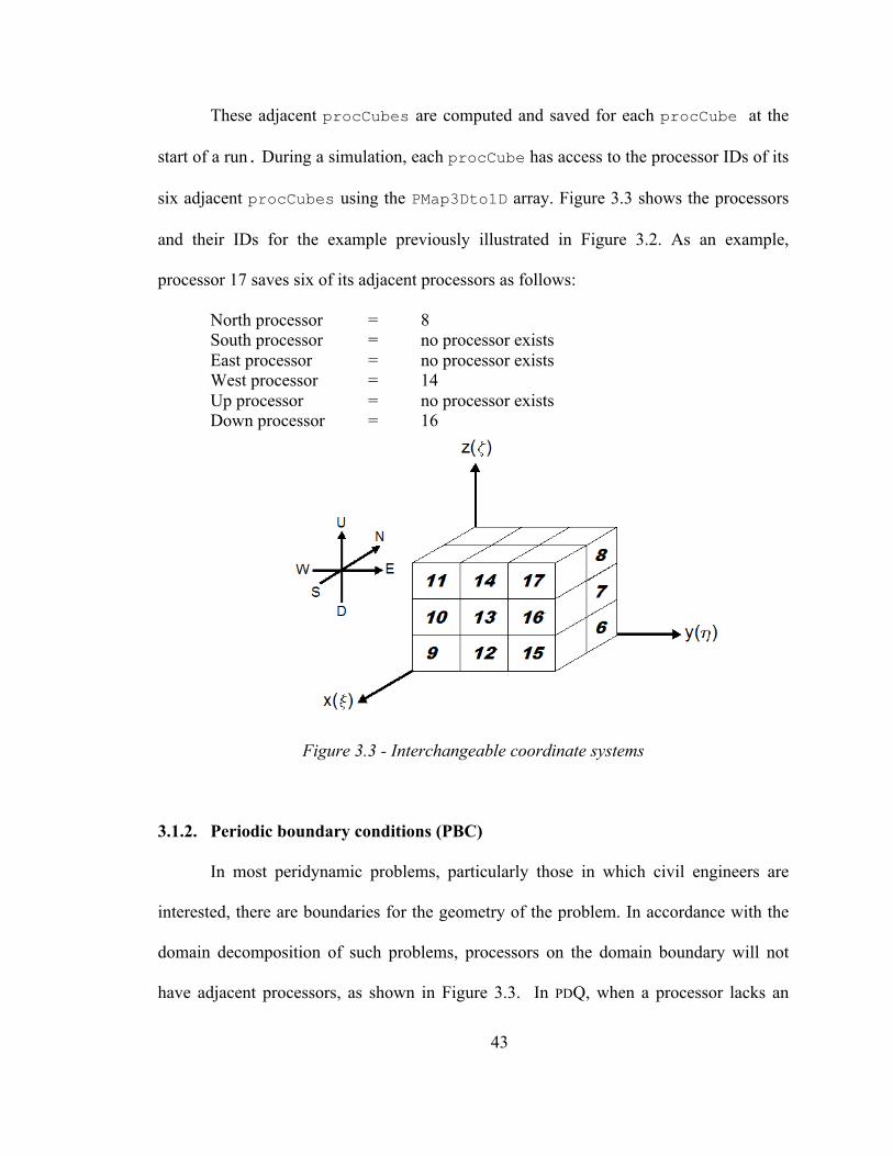
These adjacent procCubes are computed and saved for each procCube at the

start of a run. During a simulation, each procCube has access to the processor IDs of its

six adjacent procCubes using the PMap3Dto1D array. Figure 3.3 shows the processors

and their IDs for the example previously illustrated in Figure 3.2. As an example,

processor 17 saves six of its adjacent processors as follows:

North processor = 8 South processor = no processor exists East processor = no processor exists West processor = 14 Up processor = no processor exists Down processor = 16

Figure 3.3 - Interchangeable coordinate systems

3.1.2. Periodic boundary conditions (PBC)

In most peridynamic problems, particularly those in which civil engineers are

interested, there are boundaries for the geometry of the problem. In accordance with the

domain decomposition of such problems, processors on the domain boundary will not

have adjacent processors, as shown in Figure 3.3. In PDQ, when a processor lacks an

44

adjacent processor, the ID of the adjacent processor is assigned the value −1. Some

problems (mostly in molecular dynamics) are better simulated with periodic boundary

conditions (PBC) [Allen et al. 1987]. With PBC, it is assumed that the global domain is

replicated through the space in all the directions. Therefore, when a procCube lies on

the boundary of the global domain, it is surrounded by adjacent procCubes in all

directions.

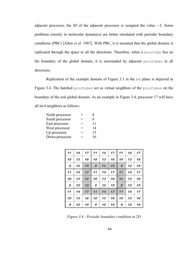
Replication of the example domain of Figure 3.3 in the y-z plane is depicted in

Figure 3.4. The hatched procCubes act as virtual neighbors of the procCubes on the

boundary of the real global domain. As an example in Figure 3.4, processor 17 will have

all its 6 neighbors as follows:

North processor = 8 South processor = 8 East processor = 11 West processor = 14 Up processor = 15 Down processor = 16

Figure 3.4 - Periodic boundary condition in 2D

45

After execution of subroutine ProcLayout in PDQ, each processor knows its

own IDs in both the 3D and the 1D coordinate systems and also knows its West, East,

South, North, Up and Down processors in either the PBC or non-PBC scheme.

3.2. Identification and mapping of cells (cell layout)

In a further level of decomposition in PDQ, each procCube is subdivided into

cuboids called cells. This is analogous to what is done in SpaSM. The function of the cell

is to facilitate keeping track of neighboring particles. As mentioned in Section 2.2.2, the

cell dimension must be slightly larger than the material horizon to guarantee that particles

interact only with particles in their containing or adjacent cells.

The cell dimension in each direction is also governed by the procCube

dimension in the same direction. The product of the cell dimension and the number of the

cells in a given direction must be exactly equal to the procCube dimension in that

direction.

In the subroutine CellLayout, each procCube is partitioned into cells. Similar

as with the procCubes, the cells are identified by two sets of IDs: an integer number for

the 1D coordinate system and three integers for the 3D coordinate system.

Mapping mechanisms, similar to those in the subroutine ProcLayout are

provided in the subroutine CellLayout. The only difference is that in the 1D coordinate

system for cell layout, the cell IDs start from one and continue to the total number of cells

in the home procCube. Such numbering prevents a cell with zero ID, facilitating array

indexing in the code. Note that zero cell IDs are avoided only in the 1D cell coordinate

system.

46

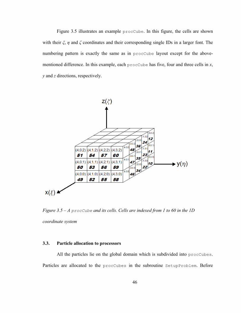
Figure 3.5 illustrates an example procCube. In this figure, the cells are shown

with their ξ, η and ζ coordinates and their corresponding single IDs in a larger font. The

numbering pattern is exactly the same as in procCube layout except for the above-

mentioned difference. In this example, each procCube has five, four and three cells in x,

y and z directions, respectively.

Figure 3.5 – A procCube and its cells. Cells are indexed from 1 to 60 in the 1D

coordinate system

3.3. Particle allocation to processors

All the particles lie on the global domain which is subdivided into procCubes.

Particles are allocated to the procCubes in the subroutine SetupProblem. Before

47

calculating acting forces, each procCube has a copy of the attributes of all the particles

in the global domain. Each procCube independently identifies the particles it contains

based on particle positions.

According to a particle’s x, y and z positions in the global domain, three IDs are

determined for each particle. These IDs are similar to procCube IDs in the 3D Cartesian

coordinate system (ξ, η, ζ) of procCubes, although in this step, they are defined for the

particles not procCubes. Similar to procCube IDs in the 3D coordinate system, their

values vary from zero to the total number of processors in that direction minus one (Nx-1,

Ny-1, Nz-1). Using PMap3Dto1D lookup array, defined in the section on processor layout

(Section 3.2), the appropriate ID in the 1D coordinate system is defined for each particle.

The processor compares the computed particle ID in the 1D coordinate system

with its own processor ID. If these IDs match, the particle belongs to that procCube and

particle information, including position, velocity, mass, material type, reference position,

etc. is copied from the global arrays into the corresponding local procCube arrays.

When reading particle information from the input files, each particle is assigned a

unique global ID which remains unchanged during the simulation. The global particle

IDs start from one and increase sequentially to the total number of particles. The purpose

of the global IDs is to keep track of particles in the global domain. The global particle

IDs are accessible within all the subroutines and should not be confused with the

computed particle IDs calculated when allocating particles to procCubes.

Particles residing of a procCube are also assigned a local ID which remains

unchanged while the particle stays on that procCube. These local IDs facilitate access to

particle atttributes in the local arrays and help to keep track of particles in the local

48

domain of a procCube. If a particle leaves a procCube and enters a new procCube, a

new local ID is assigned to it by the new home procCube.

After each processor executes the SetupProblem subroutine, the procCubes

know their contained particles and have their particle attributes in local arrays.

3.4. Particle allocation to cells (Linked List and Head arrays)

As discussed in the previous section, particles are identified in their home

procCube by their assigned local ID. Each procCube stores the particle local IDs in

two arrays: the Linked List array and the Head array. These arrays allow each particle

to recognize its cell. The Linked List and Head arrays are used to access necessary

particles and their attributes during particle interactions.

The Head array acts as the door to other particles inside each cell. The size of this

one-dimensional array is equal to the total number of the cells within a procCube. The

first element of the Head array is the local ID of an arbitrary particle on the first cell. The

second element contains the local ID of a particle in the second cell and similarly each

element of the Head array addresses to one arbitrary particle in the associated cell.

The particle local IDs from the Head array are used in the Linked List array to

access other particles in a particular cell. Each element of the Head array points to an

element in the Linked List array, which on one hand, is the particle local ID of the

next particle and on the other hand, points to the next element in the Linked List

array.

49

Figure 3.6 shows the first and second cells in a sample procCube with their

particles and their local IDs. The corresponding Linked List and Head arrays of that

procCube are also shown in the figure.

Figure 3.6 - Cells 1 and 2, Linked List and Head Arrays (Adapted from [Allen and

Tildesley 1987])

The code starts from the 1st element of the Head array. The value of 8 in the first

element, points to the particle 8 (local ID). Also it directs the code to find the next

particle of cell 1, in the 8th element of the Linked List array which is 7. Again, 7 is the

local ID of the next particle and points to 7th element of the Linked List which is 5.

The procedure will go on until the 2nd element of the Linked List points to the 1st

element which is zero. Zero value indicates that all the particles in that cell are processed.

The code will move on to the 2nd element of the Head. The procedure continues until all

the cells of a procCube are processed.

50

3.5. Interaction paths

Each particle potentially interacts with particles within all the cells adjacent to its

home cell. Each cell in each procCube knows where to look for its neighboring cells. In

other words, each cell knows which cells it interacts with. Each adjacent cell that a

particular cell needs to interact with is on the “interaction path” of that specific cell.

Subroutine DefineInteractPath defines the interaction path for each cell.

The same as with procCubes, each cell has at most 26 adjacent cells. However,

due to Newton’s third law, the interacting force between a pair of particles can be

calculated one time because the mutual force has the same magnitude but is in the

opposite direction; therefore, only one-half of the neighboring cells need be included in

the interaction path. Figure 3.7 shows the 13 neighboring cells on the interaction path of

the dark colored cell. The figure illustrates two planes of the example procCube of

Figure 3.5 separately. The illustrated pattern is analogous to the 2D interaction path

introduced in Section 2.2.2, now in three-dimensions. This interaction path following the

displayed orientation of the axes and numbering is arbitrarily defined and used in PDQ.

Figure 3.7 - Cells and their interaction paths

51

It is appropriate here to mention that the interaction paths of the cells located on

the boundary of the global domain have less than 13 cells. With PBC, all the cells, no

matter where they are located, have exactly 13 cells in their interaction paths.

Three steps are taken in DefineInteractPath to determine the interaction

paths. In the first step, six IDs are defined for each neighboring cell on the interaction

path of each cell. The first three IDs are the ξ, η and ζ coordinates of the adjacent cell

with which the home cell interacts. These coordinates are computed with the facilities

developed in cell layout (Section 3.2) and they help locating the adjacent cells on their

home procCube. To identify on which procCube each adjacent cell resides, the ξ, η,

and ζ coordinates of each adjacent cell’s home procCube are also saved which

constitutes the second stored set of IDs.

Cells located on the boundary of a procCube may have an interaction path with

cells on adjacent procCubes. A cell located on an adjacent procCube will be on its

boundary plane. A plane of cells, one cell deep, located on the boundary of a procCube,

is called a wall. According to their locations within the home procCube, these walls are

named the North, South, East, West, Up and Down walls. The boundary cells find their

adjacent cells on foreign processors through these walls. Walls are components of the

messages exchanged between adjacent procCubes. How the walls help to create the

messages is explained in detail in Section 3.6.

A wall has its own local geometric domain. Therefore, cells of a wall have

coordinates local to the domain of their home wall as well as that of the home procCube.

The ξ, η and ζ coordinates of the adjacent cells, defined in the first step, are local to their

containing procCube coordinate system. In the second step of defining interaction paths,

52

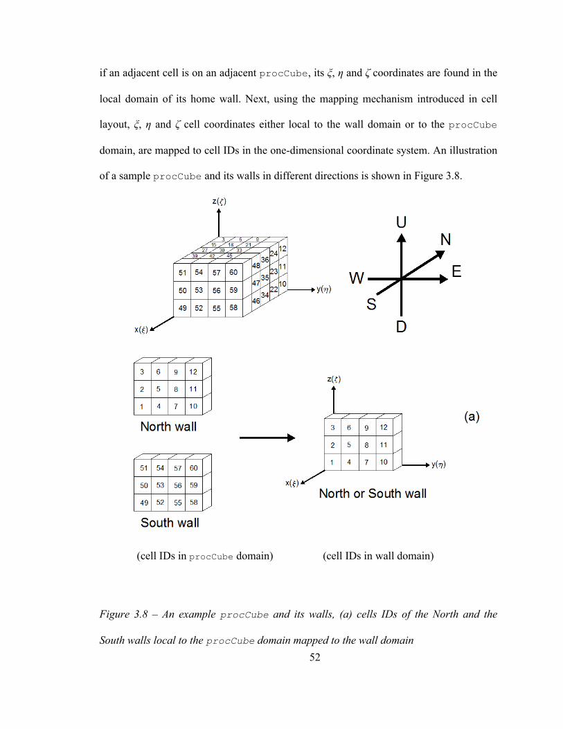
if an adjacent cell is on an adjacent procCube, its ξ, η and ζ coordinates are found in the

local domain of its home wall. Next, using the mapping mechanism introduced in cell

layout, ξ, η and ζ cell coordinates either local to the wall domain or to the procCube

domain, are mapped to cell IDs in the one-dimensional coordinate system. An illustration

of a sample procCube and its walls in different directions is shown in Figure 3.8.

Figure 3.8 – An example procCube and its walls, (a) cells IDs of the North and the

South walls local to the procCube domain mapped to the wall domain

(cell IDs in procCube domain) (cell IDs in wall domain)

53

Figure 3.8 (continued) – An example procCube and its walls, (b) cells IDs of the East

and the West walls local to the procCube domain mapped to the wall domain (c) cells

IDs of the Up and the Down walls local to the procCube domain mapped to the wall

domain

(cell IDs in procCube domain) (cell IDs in wall domain)

54

As was earlier mentioned and will be elaborated in the next section, during

processor communication, the walls constitute the components of the messages

exchanged between adjacent processors. When a wall is received from an adjacent

processor, its information is stored appropriately for later access. Therefore, a predefined

set of IDs is devised in the code for each received wall, according to its relative position

to the home procCube.

These IDs are used to store and address the indices of exchanged buffer matrices

(messages). Each ID refers to a specific location relative to the home procCube. For

instance, the adjacent procCube located to the southwest of the home procCube will be

recognized with ID number 5. Therefore, the wall received from the southwest adjacent

procCube is stored and addressed, using ID number 5. PDQ benefits from careful

assignment of these IDs to the received walls in specific order, which obviates packing

and unpacking of exchanged data.

In the final step of defining the interaction path for each cell, the interaction path

is divided into two sets. The cells which reside on the home procCube are distinguished

from those on foreign procCubes. The two matrices generated for this purpose are

PathinHomeProc and PathinAdjProc. This separation of the interaction paths is

necessary for particle interaction (Section 3.7). In addition, if fewer than 13 cells in the

interaction path are required for a particular cell (as with a boundary cell in non-PBC),

non-existing paths are excluded from the interaction path array. After the interaction

paths are defined, each cell has the local cell IDs of its adjacent cells (local to the

procCube if on the home procCube and local to the home wall if on an adjacent

55

procCube). If the interaction path points to a cell on an adjacent procCube, the

appropriate ID of that procCube is known to the home cell.

3.6. Particle communication

If a processor needs information located on an adjacent processor, message

passing is required. The necessary data is delivered from the source processor to the

asking processor. Message passing is enabled by the physical network links that are

provided in the architecture of the multi-node machine connecting all the processors to

each other.

To calculate the forces acting on particles, each particle must interact with its

neighboring particles. However, some of these neighboring particles are located not on

the home procCube, but on adjacent procCubes. Therefore, the necessary information

must be received by the home processor. The subroutine ParticleComm is responsible

for sending and receiving the necessary data using MPI commands.

A procCube is potentially surrounded by up to 26 procCubes, which implies

that 26 messages are needed for each processor in each time step. With Plimpton’s

method of message passing (Section 2.2.4), all the data is sent by only six messages.

Taking full advantage of Newton’s third law further reduces the 6 messages to 5.

According to the interaction paths shown in Figure 3.7, a cell never asks for information

from its North (-x direction) plane. Therefore, if a cell is on the edge of a procCube,

there is no need for the information of the adjacent cells on its North plane, which is the

“south” wall of the “north” procCube. Consequently, there is no need to exchange the

“south” walls between the processors and the necessary messages are reduced to 5.

56

The concept of the walls is used in PDQ combined with Plimpton’s method of

message passing. The messages are, in fact, composed of the walls. Walls are received in

buffers which are constructed in such a way that their particles’ home cells and home

procCubes are known. The structure of buffer matrices has been explained in

interaction paths. As explained in Section 2.2.4, the idea of Plimpton’s method is that in

some steps of message passing, some parts of received buffers are sent themselves as

messages. Thus, each procCube potentially works as the source to send a message, as

the destination to receive a message and also as a transmitter, i.e., it relays some of the

received messages to other procCubes.

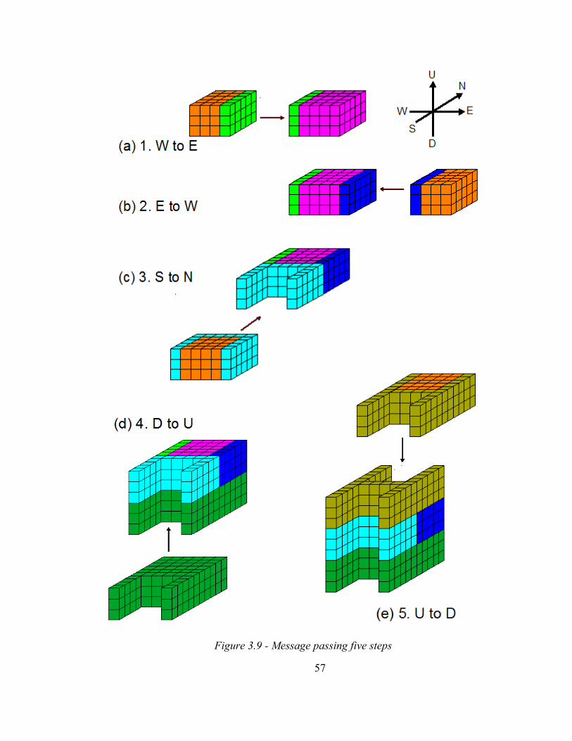
In PDQ, all of the procCubes receive all the information they need in five steps

(messages). Figure 3.9 shows how necessary messages are received by the purple object

which is assumed to represent the home procCube. The orange objects are neighboring

procCubes. It is very important to note that the figure only illustrates how the messages

are received by the purple procCube. However, the purple procCube also sends its

information to its adjacent procCubes as well, and the identical procedure is performed

simultaneously by all of the procCubes, in parallel.

57

Figure 3.9 - Message passing five steps

58

In the first step, simultaneously, all procCubes send their East walls to their East

procCube and receive a wall from their West procCube. After the first step, all the

procCubes have the received the wall of their East procCube which is saved in the

appropriate place in the receiving procCubes. This is illustrated graphically in Figure

3.9a where the green wall, sent by the East processor, is attached to the home procCube.

The second step involves exchange of information in the East-to-West direction.

Each procCube sends its West wall to the West procCube and receives a wall from the

East. After the second step, the procCubes have received walls from West and East

procCubes. In Figure 3.9b the blue wall represents the received buffer from the East by

the home procCube.

In the third step of message passing, all procCubes send the North walls to their

North procCubes and receive walls from the South. In this step, the size of the message

is roughly three times the size of the messages exchanged in the E-W and W-E message-

passing steps, because the message includes three walls: the North wall of the South

procCube as well as the walls previously received from the East and West procCubes

of the South procCube. Thus the home processor receives the North wall of its South

processor and the East and West walls of the processors located on southwest and

southeast of the home processor in one package. Figure 3.9c shows the received message

from South procCube in light blue.

In the third step of message passing, as well as fourth and fifth steps, procCubes

not only send and receive data they need, but also send previously received walls to

adjacent procCubes.

59

From the walls received from southeast and southwest procCubes, the home

procCube requires only a column of the cells which are shown in yellow in Figure 3.10.

The rest of the cells of the walls, received from southeast and southwest procCubes, are

not required, although they are exchanged.

.

Figure 3.10 – Third step of receiving adjacent walls, necessary columns from southeast

and southwest procCubes shown in yellow

The fourth message, shown in Figure 3.9d, contains six walls: the walls

previously received by the Down procCube from its East and West in the first step,

three walls received by the Down procCube from South as explained in step three, and

the up wall of the Down procCube. All of this information is sent in one pack of data

(one message) by the Down procCube. Simultaneously, the home procCube sends such

information to its own Up procCube.

The last step is similar to the fourth one. Six walls, including five walls previously

received from nearby procCubes, along with the Down wall of the Up procCube are

sent down and received by the home procCube. At the end of the final step all the

procCubes have received the necessary data (Figure 3.9e).

As noted earlier, due to Newton’s third law, there is no need for data exchange in

the direction of North to South which reduces the number of messages to five. As

60

explained before, benefiting from Newton’s third law obviates exchange of information

from North to south.

Every procCube needs only the information in the boundary cells of adjacent

procCubes which creates one cell-deep shell around the home procCube. However, as

illustrated in Figure 3.9e, some unneeded cells are transferred to the home procCube. In

fact, there is a surfeit of exchanged data. More research is required to determine if, in this

particular method, the advantage of a reduced number of messages outweighs the

disadvantage of passing more information than is absolutely required.

3.7. Particle interaction

This section explains how particle interacting forces are calculated. Subroutine

Interact does this in three steps. In the first step, all the particles, that reside on a

specific cell and are within the material horizon of each other, interact. In the second step,

the interactions between a particle and the neighboring particles which lie outside the

home cell but within the home procCube are computed. Such particles are accessible by

PathinHomeProc, constructed in defining interaction paths. In both steps, the

interacting particles are within the home procCube and all required information to

calculate the interaction forces is accessible via local arrays. In the final step of

interaction, cells having interaction paths on adjacent procCubes interact with those

adjacent cells. These interaction paths have been previously stored in array

PathinAdjProc. The predefined IDs introduced in the second step of defining

interaction paths are used to find the appropriate data through buffer arrays. At the end of

61

this step, all inter-particle forces on all particles have been calculated for the specific time

step.

Benefiting from Newton’s third law, only half of the interaction forces need be

calculated. Each interaction force has a mutual force with the same magnitude and

direction but with opposite sign. These mutual forces must be added to the total force

acting on the other particle. For the interactions inside the home procCube, the reaction

forces are added to local force arrays immediately after the calculation of the interaction

forces. For interactions with particles on foreign procCubes, the mutual forces are

stored in specific buffer arrays called ForceAdjBuf. These arrays are sent to adjacent

procCubes, where the corresponding particles reside. On home procCubes, received

mutual forces are added to local force arrays to sum the total forces acting on each

particle.

3.8. Message components (beams, columns, and cornices)

The most efficient code sends and receives the least number of messages which

contain only the necessary data. Reducing the number of exchanged messages decreases

the computation latency (Section 2.2.4). Latency is largely a function of the speed of

light, and in most fiber optic cables it results in about 4.9 microseconds of latency for

every kilometer. One of the wall message-passing method’s strengths is that it reduces

the number of necessary exchanged messages to 5 as opposed to 6 in Plimpton’s original

method. However, there is a surfeit of data exchanged in this method which might

counterbalance its speed. It is unclear how these two factors balance each other.

Clarifying this issue requires further research.

62

The size of the messages can be reduced by sending only the necessary data. To

prevent over-sending information, new objects with a similar functionality as with the

walls should be defined. In consistent with previous naming convention, these objects can

be names beams, columns, and cornices. Figure 3.11 illustrates these objects, where the

walls are colored cyan, columns are yellow, beams are orange and cornices are shown

green.

Figure 3.11 – Walls, beams, columns and cornices are components of the messages

Using these objects in creating the messages adds another step to forming the

messages. The messages must be packed appropriately before sending and be unpacked

in the destination procCube. There are predefined MPI commands for packing and

unpacking data. However, packing and unpacking of data, while reducing communication

time, require more computation time. More research is required to determine if doing so

will speed up the code.

63

3.9. Force communication

As was discussed in previous section, the mutual forces calculated on foreign

procCubes are sent to associated procCubes. Subroutine ForceComm is responsible

for sending and receiving force buffer arrays which contain the mutual reaction forces.

The same message-passing idea used in particle communication is implemented in

force communication with some alterations. The process involves sending and receiving

five messages in the reverse process as for the particle communication procedure (Section

3.6). The only difference is that in each step of message passing, the receiver processor

adds up the forces acting on particles received from different sender processors.

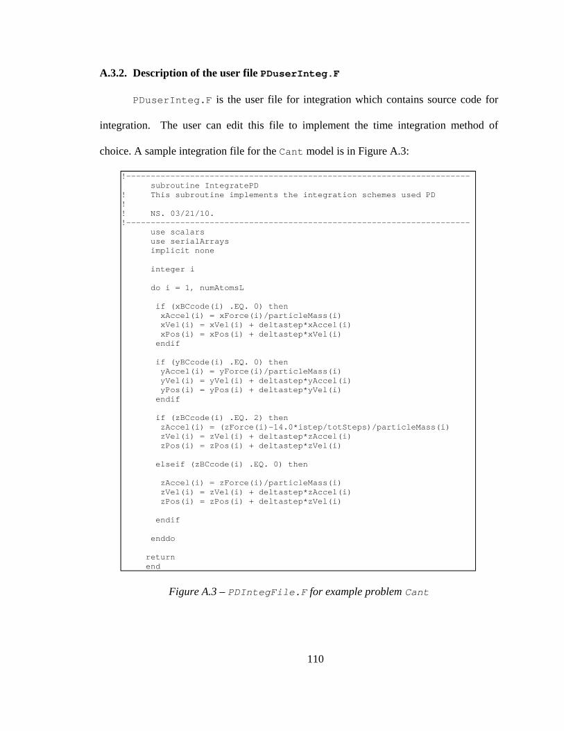
3.10. Integration

After calculating the total force acting on all particles, the positions and velocities

of all the particles are updated in the integration subroutine. Using Newton’s second law,

its acceleration of every particle is calculated based on its mass and the applied force. The

updated velocity is computed given the acceleration and velocity at the previous time

step. The particle position is updated using the new velocity and previous position.

There are several integration methods in the literature. The molecular dynamics

mode in PDQ offers two options: the “Velocity Verlet” integration method and the

“Leapfrog” method. Other methods include finite difference methods such as the

“predictor-corrector” algorithm, the “Gear predictor-corrector” algorithm and the

“Runge-Kutta-Gill” method [Allen and Tildesley 1987]. The integration source code file

in peridynamics mode of PDQ is exposed to the user to enable alternative integration

scheme to be replaced.

64

3.11. Particle shuffling

A necessary feature for the code is particle shuffling. This involves

transferring particles to new procCubes and cells. When particle displacements are not

negligible compared to the radius of interaction, particles may leave their home

procCubes and cells and move into adjacent procCubes and cells. It is necessary to

transfer particles from their home procCube (to which the particles originally belong)

to new procCubes. This involves deleting alterable particle attributes from the local

arrays of the home processor, and inserting this information to the new processor local

arrays. Relocation of particles to an adjacent procCube is possible for particles lying on

the walls of the procCubes. Currently, the developed parallel algorithm is being revised

to address particle shuffling in PDQ. Particle shuffling is very important particularly for

molecular dynamics simulations, wherein large displacements, compared to the cutoff

distance of the particles, occur.

3.12. Generalization of degrees of freedom

Modifying PDQ to handle user-defined degrees of freedom is a necessary

feature of PDQ which gives PDQ unique generality and flexibility. Several steps need to

be done to supply this capability to PDQ. The most important step, which has been

implemented in the current version of PDQ, involves modifying the communication

subroutines, ParticleComm and ForceComm. These subroutines basically contain MPI

send and receive commands. The indices of arrays and array sizes, which are to be

exchanged, are pre-calculated based upon the number of degrees of freedom of the

65

problem. In peridynamics simulation, number of degrees of freedom is an input

parameter in the main input file. Its value is set to three as a default value for molecular

dynamics simulations. A new extension of PDQ has been developed which fully addresses

generalized degrees of freedom for peridynamics simulations. Solving similar problems

with available versions showed a slowdown in calculation time. The latest version seems

to be more than three times slower than the original version. This reduction in speed is

expected as the modified version utilizes multi-dimensional arrays for particle and force

field attributes instead of one-dimensional arrays used in the original version of PDQ.

Processors spend more time on calculating the address of a certain element of a multi-

dimensional array in the memory. Memory address finding process takes place much

quicker for one-dimensional arrays. Further research is required to minimize the effect of

using multi-dimensional arrays on the speed of the code.

3.13. Summary

The wall method message passing algorithm was explained in this chapter. In

addition, details of the parallel scheme used in PDQ and the implementation of the wall

method message passing were described.

The source code in peridynamic mode of PDQ is divided into two sections. The

main source code contains the parallelization scheme where it takes place behind the

user’s eye. Some of the source code is open to the user to define desired force field and

integrating method. Editing these files does not require any knowledge of the

parallelization method. To help the user to edit these source code files, create necessary

input files and analyze the outputs, a user manual is provided.

66

Several example problems are simulated using PDQ which are presented in the

next chapter. The user is able replicate the simulated problems using the user manual

(Appendix A).

67

4. EXAMPLE PROBLEMS

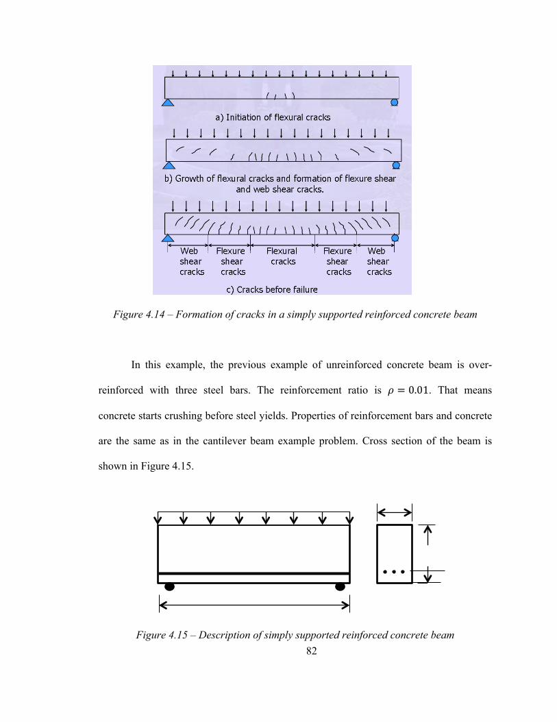
This chapter presents the results from six example problems in civil engineering

simulated using PDQ. The example problems include a plain and a reinforced (RC)

concrete cantilever beam, a plain and a reinforced simply supported concrete beam, a lap

splice pullout problem and a prestressed (PS) bulb T beam. The first four problems are

canonical, relatively simple problems in structural analysis for which the strength can be

simply calculated from solid mechanics equations. The lap splice pullout problem was

previously simulated by Gerstle, Sakhavand and Chapman [Gerstle et al. 2010] using

EMU. The shear failure mechanism of a prestressed bulb T beam is a problem of interest

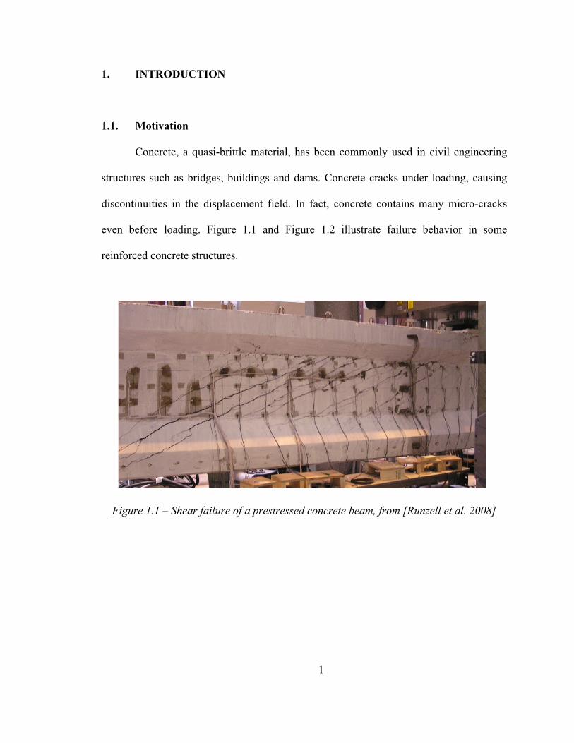
to many civil engineers. Figure 1.1, in the Introduction section of this thesis, illustrates

shear cracking of a prestressed concrete beam under loading in a laboratory test.

The presentation of these results serves two purposes: validating the code, and

demonstrating the range of problems that can be tackled using peridynamics.

For all these problems, the initial minimum and maximum natural frequency of

vibration of the problem is determined using a commercial finite element simulation

package, SAP2000 11.0.8 (Computers and Structures, Inc., Berkeley, California). The

total duration of the simulation is determined based on the minimum natural frequency.

The maximum frequency is used to determine the time step of the problem in the

preprocessing step (Appendix A).

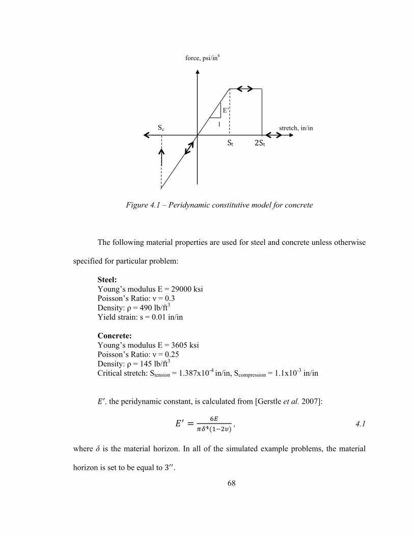
Both concrete and steel are treated as nonlinear elastic, but this should not matter

if no unloading of links occurs. The constitutive model used in the simulations for

concrete is shown in Figure 4.1.

68

Figure 4.1 – Peridynamic constitutive model for concrete

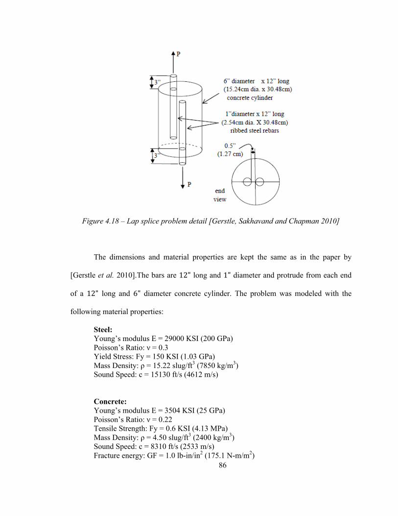
The following material properties are used for steel and concrete unless otherwise

specified for particular problem:

Steel: Young’s modulus E = 29000 ksi Poisson’s Ratio: ν = 0.3 Density: ρ = 490 lb/ft3 Yield strain: s = 0.01 in/in Concrete: Young’s modulus E = 3605 ksi Poisson’s Ratio: ν = 0.25 Density: ρ = 145 lb/ft3 Critical stretch: Stension = 1.387x10-4 in/in, Scompression = 1.1x10-3 in/in !!, the peridynamic constant, is calculated from [Gerstle et al. 2007]:

!! = !!!!!(!!!!)

, 4.1

where δ is the material horizon. In all of the simulated example problems, the material

horizon is set to be equal to 3!!.

force, psi/in6

stretch, in/in

1

E’

Sc

St

2St

69

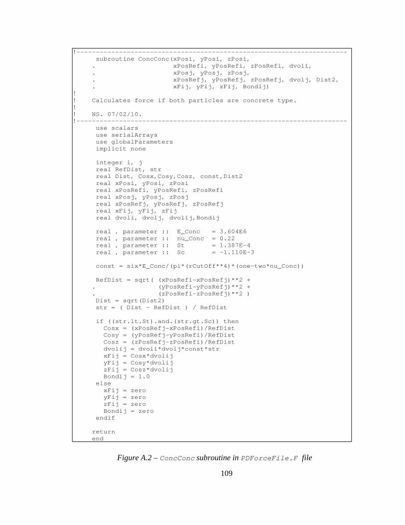
Figure 4.2 shows the peridynamic pairwise force function for steel.

Figure 4.2 – Peridynamic constitutive model for steel

To simulate the bond-slip behavior between the steel bars and the concrete, the

interaction between steel and concrete particles is simulated as concrete-concrete except

that the calculated pairwise force and the critical stretches are both multiplied by a factor

of three. This is the recommended factor in the EMU user manual.

Black regions in the figures illustrate particles having more than specified

percentage of broken links. A link breaks when the previously existing interacting force

between a pair of particles turns zero. Post-processing tools allow choosing the specified

percentage of damaged links.

All the simulations were performed on the nano Linux parallel supercomputer at

the University of New Mexico Center for Advanced Research Computing (CARC).

nano’s specifications are as follows:

• Dell PowerEdge 1950 nodes

force, psi/in6

stretch, in/in

1

E’

Sc

St

Fy

Fy

70

• 36 nodes each with dual 2.33 GHz dual core Intel Xeon processors

• 144 processors total

• 8 GB/node of local memory (RAM)

• 73 GB/node of local disk

• Myrinet2 Interconnect for fast inter-node communication

• 3 TB temporary scratch storage

In general, not all nodes are available for production computing. One node is

reserved for debugging purposes and one node is reserved for maintenance.

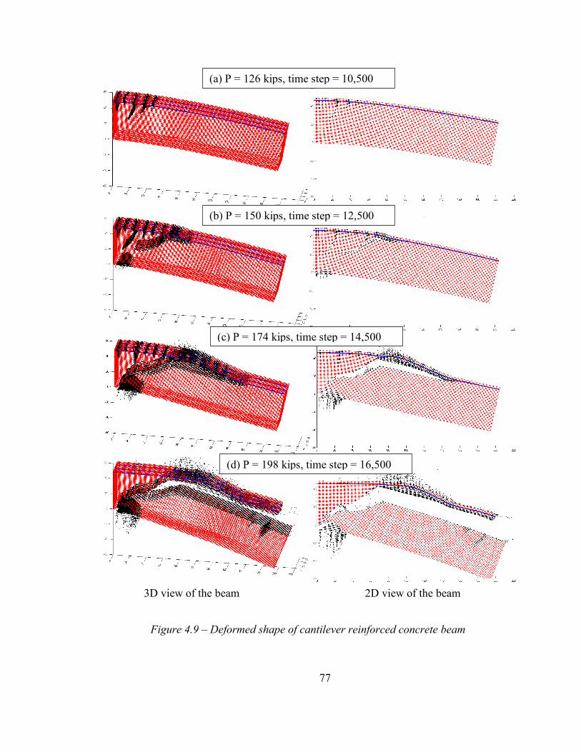
4.1. Plain concrete cantilever beam

In the first example, a 3D concrete beam, subjected to a downward force (Figure

4.3), is simulated with PDQ. A similar 2D example was previously simulated by Sau [Sau

2008] with a different peridynamic model on a single processor. Sau states that solving

such a problem requires a lot of memory and computer run time [Sau 2008], suggesting

that this might be a good test problem for PDQ on a parallel supercomputer.

The simulated problem is a three-dimensional concrete beam of 200" length, with

a rectangular cross section of 30" wide and 50" deep. Three planes of particles in the

cross section of the beam are constrained in all the directions at the left end. The problem

consists of a cubical grid of 200×50×30 = 300,000 particles spaced at 1" with a

material horizon of 3".

The model is subjected to a uniform force at the free end of the beam. The

external force is applied to two planes of particles at the right end. The total applied force

P is calculated as follows:

71

! = !"#$%!"#$%&'(

× !"!#$ !"#$%& !" !"#$%$ !"#$%&'() = 2×50×30 . 4.2

The model is illustrated in Figure 4.3.

Figure 4.3 – Description of cantilever plain concrete beam

In a mechanics of material analysis, the maximum stress forms at the fixed end of

the beam and is calculated as:

!!"# = !.!!= !.!.!

!, 4.3

where ! is the resulting moment, ! is the moment of inertia of the cross section, ! is the

total length of the beam, ! is the total applied load and ! is the half vertical length of the

cross section.

The fracture strength of concrete is computed from:

!! = 7.5 !!!, 4.4

where f!! is the 28-day compressive strength of concrete.

P

200"

30"

50"

72

With L = 200", f!! = 4000 psi, c = 25" , I = !"!!!"!"

= 312500 in4, and by

substituting f! from Equation 4.4 in Equation 4.3, it is estimated that the beam should

start cracking at P = 30 kips.

The force is linearly increased as a function of time shown in Figure 4.4.

Figure 4.4 – Applied force vs. time

The simulation time step is 0.34×10!! sec. A magnified 100x view of the beam

deformation at different time steps is shown in Figure 4.5. The applied force at each

particular time step is shown in each frame. Particles with 20% or more damage are

shown in black. The beam suddenly starts cracking when the applied force approaches 30

kips.

Time (sec)

Force (kips)

42 kips

73

Figure 4.5 – Deformed shape of cantilever plain concrete beam using PDQ

P = 28.0 kip

P = 29.4 kips

P = 30.8 kips

P = 32.2 kips

(a) time step = 20,000

(b) time step = 21,000

(c) time step = 22,000

(d) time step = 23,000

74

Figure 4.6 shows absolute value of the displacement of a point located at the

bottom right side of the beam, drawn according to the applied force. As the load is

increased, the magnitude of the displacement is consequently increased. At the time the

beam reaches its ultimate strength, the rate of change of displacement starts to increase

and the displacement approaches an infinite value.

Figure 4.6 – Displacement vs. force plot

The value of the ultimate load estimated from Figure 4.6 is comparable to the

calculated strength of the beam from the mechanics of materials equations.

4.2. Reinforced concrete cantilever beam

This is the same as problem number one except that the beam is now reinforced

with three steel bars. The reinforcement ratio is 0.014. Figure 4.7 shows details of the

model.

! ≈ 30 !"#$

75

Figure 4.7 – Description of cantilever reinforced concrete beam

The model consists of 300,600 particles located in a box grid of one-inch spacing.

The boundary conditions are similar to the previous example problem. Three planes of

particles in the cross section of the beam are restrained from moving in all the directions

on the left side. The load is applied to two planes of particles on the right side of the bam.

The American Institute of Concrete (ACI) design code specifies that the shear

strength of a reinforced concrete beam can be calculated from:

!! = 2 !!!!!!. 4.5

With b = 30", f!! = 4000 psi, and d = 46.5", the maximum shear strength of the

beam is predicted as V! = 175 kips.

Similar to the first example, a force linearly increasing by time (Figure 4.4), is

applied to two planes of particles at the right end of the beam.

30" P

200"

50"

3.5"

10” 10”

76


The simulation time step is 0.18×10!! sec, which is smaller than the plain

concrete example, because steel increases the strength of the beam, thus decreasing the

minimum period (! = !!= !!

!).

Snapshots from 100x magnified deformation of the cantilever beam at different

time steps are shown in Figure 4.9. Particles with more than 20% damage are shown in

black. For clarity, only the outer periphery of concrete is shown in the figure. Figures on

the left are 3D view of the same time step which is shown on the right in 2D.

Time (sec)

Force (kips)

240 kips

77

Figure 4.9 – Deformed shape of cantilever reinforced concrete beam

(a) P = 126 kips, time step = 10,500

3D view of the beam 2D view of the beam

(b) P = 150 kips, time step = 12,500

(d) P = 198 kips, time step = 16,500

(c) P = 174 kips, time step = 14,500

78

Propagation of flexural and shear cracks are observed in Figure 4.9. Crushing of

concrete also is visible at the left bottom corner of the beam. The simulation took

approximately 3 hours to run on nano using 32 processors.

The absolute value of the displacement of a particle located at the bottom right

corner of the beam is shown in Figure 4.10, according to the increasing applied force.


Such displacement vs. force plot can be used to determine strength of a beam.

Sudden change in the rate of increase of the displacement takes place when the beam is

not able to hold any larger loading (ultimate strength of the beam). The estimated value

of the ultimate strength from the displacement vs. force plot (180 kips) is comparable to

the ultimate shear strength computed using ACI equations (175 kips).

! ≈ 180 !"#$

79

4.3. Simply supported plain concrete beam

The failure of a simply supported concrete beam is a famous problem in fracture

mechanics. The beam is simulated using PDQ and is subjected to a uniform load applied

at the top of the beam. The model description is shown in Figure 4.11.

Figure 4.11 – Description of simply supported plain concrete beam

The beam consists of 375,000 particles with 1” spacing between particles. The

problem is simulated with the pairwise force function shown in Figure 4.1.

As the maximum stress happens at the bottom middle of the beam, it is expected

that first cracks will nucleate in that area. The maximum normal stress is:

!!"# = !!"#.×!

!. 4.6

The fracture strength of concrete is computed from:

!! = 7.5 !!! 4.7

From classical beam theory, the maximum moment and shear for a simply

supported beam are:

!! = !×!!

!, !! =

!×!!

4.8

w

250"

30"

50"

80

With L = 250", f!! = 4000 psi, c = 25" , I = !"!!!"!"

= 312500 in4, and by

substituting f! from Equation 4.7 in Equation 4.8, the strength of the beam is calculated

as w = 760 lb/in.

The beam is under a uniform force applied at two top layers of the particles. The

force is increased linearly as the simulation advances.


The deformed shape of the beam using PDQ is shown in Figure 4.13. Each frame

shows a snapshot of the simulation at a certain time step and includes the applied force at

that time step. Particles with 20% or more damage are shown in black. The deformation

is magnified 100 times. As shown in Figure 4.13, a sudden failure occurs when the load

reaches to 765 lb/in, which is comparable to the calculated strength of 760 lb/in.

Time (sec)

Force (lb/in)

900 lb/in

81

Figure 4.13 – Simulation results of simply supported plain concrete beam

4.4. Simply supported reinforced concrete beam

Studying shear failure mechanism in a reinforced concrete beam is an interesting

area of research which has led to the development of shear provisions in the civil

engineering design codes such as ACI and AASHTO. Figure 4.14 shows formation and

propagation of shear cracks in a simply supported reinforced concrete beam.

(c) w = 810 lb/in, time step = 18,000

(b) w = 765 lb/in, time step = 17,000

(a) w = 720 lb/in, time step = 16,000

82

Figure 4.14 – Formation of cracks in a simply supported reinforced concrete beam

In this example, the previous example of unreinforced concrete beam is over-

reinforced with three steel bars. The reinforcement ratio is ! = 0.01. That means

concrete starts crushing before steel yields. Properties of reinforcement bars and concrete

are the same as in the cantilever beam example problem. Cross section of the beam is

shown in Figure 4.15.

Figure 4.15 – Description of simply supported reinforced concrete beam

83

The ACI specifies that the shear strength of a concrete beam can be calculated

from:

!! = !! = 2 !!!!!!, 4.9

where !! is the width of the beam, d is the distance between steel bars and farthest in-

compression fibers of concrete, and !!! is the 28-day strength of concrete.

With !! = 30", !!! = 4000 psi, and ! = 46.5", the maximum shear strength of

the beam is calculated approximately as !! = 175 kips. The beam is subjected to a

uniform force at the top which is increasing proportional to the time.

If Vc equals the maximum nominal shear force Vu, the value of the uniform

applied force, w, which produced Vc will be:

! = !!!!= !×!"#$$$

!"#= 1400 !"

!" 4.10

A uniform force, which is a linear function of time, is applied to the two top

layers of particles. Nucleation and propagation of shear cracks are observed as shown in

Figure 4.16.

84

Figure 4.16 – Deformed shape of simply supported reinforced concrete beam using PDQ

w = 1020 lb/in

w = 1080 lb/in

w =1160 lb/in

w = 1240 lb/in

w = 1260 lb/in

85

The absolute value of the displacement of a particle located at the middle top of

the beam is plotted against the time (Figure 4.17). The displacement becomes unstable at

the time when force is approximately 1300 lb/in. This value can be compared to the

calculated strength of 1400 lb/in.


4.5. Lap splice pullout

Gerstle, Sakhavand and Chapman [Gerstle, Sakhavand and Chapman 2010]

simulated the reinforced concrete lap splice problem in 2010 using EMU. The results

were compared to a finite element model using ANSYS (ANSYS, Inc., Canonsburg,

Pennsylvania) and experimental laboratory tests. The same problem is solved using PDQ

and the results are compared. The problem consists of a cylinder of concrete with two

bars embedded in the concrete as shown in Figure 4.18.

! ≈ 1300 !"/!"

86

Figure 4.18 – Lap splice problem detail [Gerstle, Sakhavand and Chapman 2010]

The dimensions and material properties are kept the same as in the paper by

[Gerstle et al. 2010].The bars are 12" long and 1" diameter and protrude from each end

of a 12" long and 6" diameter concrete cylinder. The problem was modeled with the

following material properties:

Steel: Young’s modulus E = 29000 KSI (200 GPa) Poisson’s Ratio: ν = 0.3 Yield Stress: Fy = 150 KSI (1.03 GPa) Mass Density: ρ = 15.22 slug/ft3 (7850 kg/m3) Sound Speed: c = 15130 ft/s (4612 m/s)

Concrete: Young’s modulus E = 3504 KSI (25 GPa) Poisson’s Ratio: ν = 0.22 Tensile Strength: Fy = 0.6 KSI (4.13 MPa) Mass Density: ρ = 4.50 slug/ft3 (2400 kg/m3) Sound Speed: c = 8310 ft/s (2533 m/s) Fracture energy: GF = 1.0 lb-in/in2 (175.1 N-m/m2)

87

The lap splice problem is in dynamic, not static, equilibrium. The top part of the

bar protruding from the top of the concrete is subjected to a uniform upward velocity of

7.87 in/s during the run. Similarly, the bottom part of the bar protruding from the bottom

of the concrete is subjected to a uniform downward velocity of 7.87 in/s. The protruding

parts of the bars are restricted from moving in the plane of cylinder base.

Figure 4.19 shows some figures from the simulation using EMU [Gerstle et al.

2010]. The black particles show damaged regions.

88

Figure 4.19 - Undeformed and deformed shapes at three simulation times from EMU [Silling 2003]. Deformation is magnified by a scale factor of 50. Particles with more than 30% of peridynamic links being broken are displayed as black [Gerstle, Sakhavand and Chapman 2010].

t = 0.00072 s

(a)

t = 0.0014 s (b)

t = 0.0022 s (c)

89

The lap splice pullout problem is also simulated using PDQ. The peridynamic

constitutive model (pairwise force and stretch relationship) used for concrete is shown in

Figure 4.1. The material properties are the same as used in EMU.

There are certain differences between the codes. EMU uses state-based

peridynamic model (Section 2.1.2) whereas the results from PDQ are based on the

original bond-based peridynamic theory. Figure 4.20 shows the results of the lap splice

problem using PDQ subjected to a 7.87 in/sec velocity applied in opposite direction to the

protruding sections of steel bars.


particles with more than 35% or more damage are shown in black

time step = 3000 t = 0.0005 sec

time step = 4000 t = 0.0007 sec

time step = 5000 t = 0.0009 sec

90

The time step used is 0.18×10!! sec. Comparing figures from EMU simulations

to those from PDQ simulations, shows that cracking pattern starts similarly and diverges

as the simulation moves forward. Comparison of the figures according to their time step

shows that propagation of cracks occurs much faster in PDQ than in EMU. Although the

same parameters used in EMU have been used in PDQ for simulating this problem, the

force fields might be different. The parameters used in the force filed in EMU are not

clearly defined, thus using different parameters might account for the discrepancy in the

results.

The same problem has been solved with a slower applied velocity (2.00 in/sec).

The results are shown in Figure 4.21.



time step = 5000 t = 0.0009 sec

time step = 7000 t = 0.0012 sec

time step = 9000 t = 0.0016 sec

91

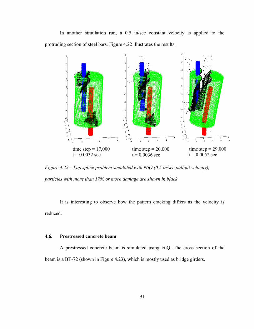
In another simulation run, a 0.5 in/sec constant velocity is applied to the

protruding section of steel bars. Figure 4.22 illustrates the results.



It is interesting to observe how the pattern cracking differs as the velocity is

reduced.

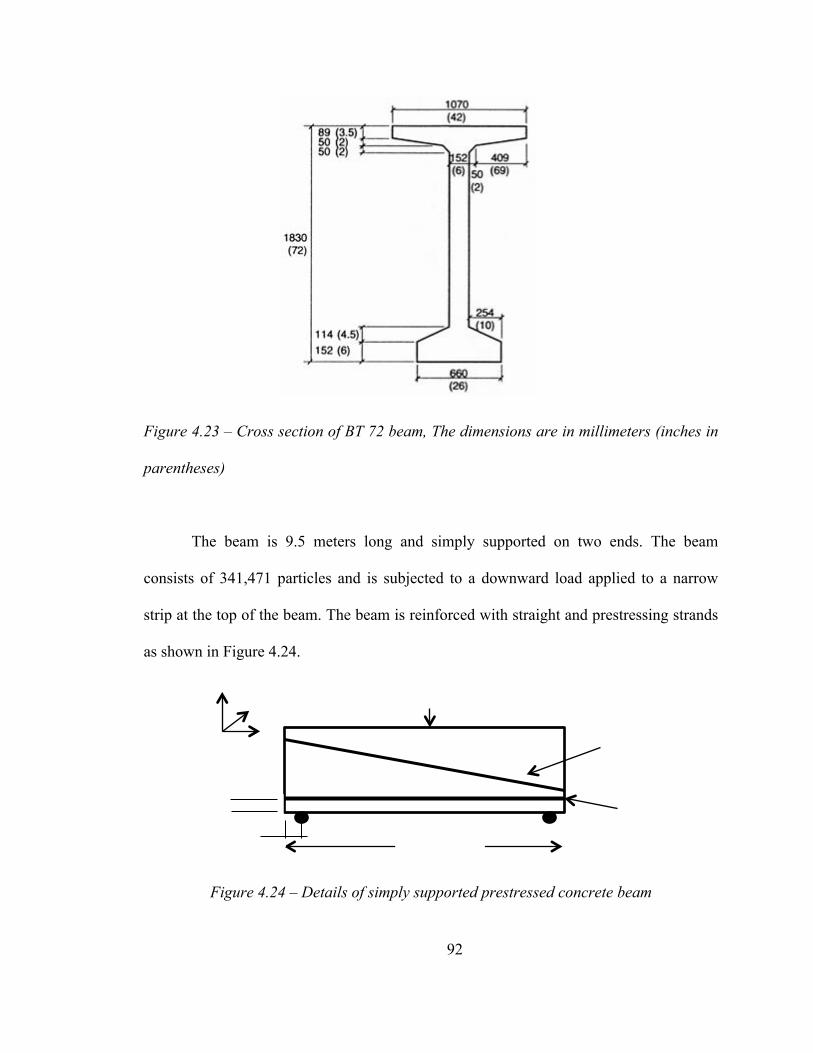
4.6. Prestressed concrete beam

A prestressed concrete beam is simulated using PDQ. The cross section of the

beam is a BT-72 (shown in Figure 4.23), which is mostly used as bridge girders.

time step = 17,000 t = 0.0032 sec

time step = 20,000 t = 0.0036 sec

time step = 29,000 t = 0.0052 sec

92

Figure 4.23 – Cross section of BT 72 beam, The dimensions are in millimeters (inches in

parentheses)

The beam is 9.5 meters long and simply supported on two ends. The beam

consists of 341,471 particles and is subjected to a downward load applied to a narrow

strip at the top of the beam. The beam is reinforced with straight and prestressing strands

as shown in Figure 4.24.

Figure 4.24 – Details of simply supported prestressed concrete beam

93

The pattern of reinforcing strands is shown in Figure 4.25. Eight reinforcing bars

and three prestressing strands are inserted in the beam. Each reinforcing bar has an area

of 400 mm2 and each prestressing strand has an area of 450 mm2.

Figure 4.25 – Details of the strands in the prestressed bulb T beam

Two lines of particles in the x-direction and two lines in the z-direction are

restrained from moving in z-direction. The top middle strip of the beam (two lines of

particles in x-direction and two lines of particles in z-direction) are subjected to a

downward force, P.

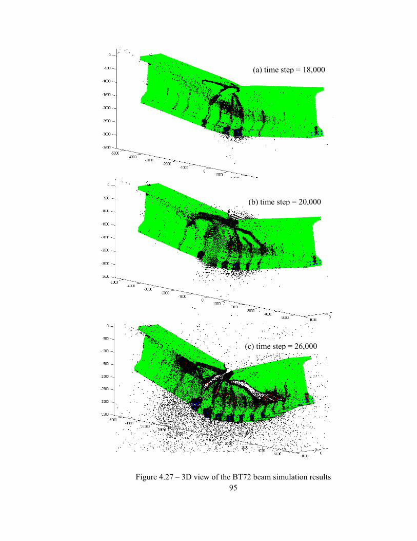
The deformed beam is shown in Figure 4.26 and Figure 4.27 at different time

steps. The black particles show particles with more than 10% damage. The deformation

is magnified 100 times. The time step used in this simulation is 0.18×10!! sec.

100 mm

160 mm

prestressing strands

94

Figure 4.26 – 2D view of the BT72 beam simulation results




95

Figure 4.27 – 3D view of the BT72 beam simulation results




96

Cracking starts with the flexural cracks in the bottom flange. As the simulation

advances, shear cracks nucleate and propagate in the web of the beam. In this example,

the simulation results from PDQ are qualitatively presented. Quantitative comparison can

be done by incorporation of ACI code provisions for designing prestressed girders used

in bridges.

4.7. Scalability and timing performance

Scalability is how the performance of a system, network or process changes in

accordance with the increased load. Consequently, a scalable system is a system whose

performance improves proportionally with the hardware added.

As computational hardware prices drop, low-cost commodity systems are

increasingly used for high-performance computing. The parallelization algorithms used

for parallel particle-based simulations are desired to scale, i.e., they must be suitably

efficient and practical when applied to simulations of a large number of particles. In the

context of high performance computing, speedup refers to how much a parallel algorithm

is faster than a serial algorithm. Speedup is defined by Equation 5.11.

! = !!!!

, 4.11

where S is speedup, Ts is the calculation time using one processor and Tp is the

calculation time using a parallel algorithm for a specific number of processors.

In an ideal scalable algorithm, calculation time is inversely proportional to the

number of processors used, for the same problem with the same size. Figure 4.28 shows

the calculation time per 1000 time steps against number of processors for the lap splice

pull out problem with 362,677 particles.

97

Figure 4.28 – Speedup for the lap splice pullout problem with 362677 particles

Gerstle et al. [Gerstle, Sakhavand and Chapman 2010] tried to estimate the total

simulation time of a given problem in EMU using Equation 5.11:

! = !× !×!!

, 4.12

where K is processor-seconds per particle-time step, P is the number of processors, N is

the total number of particles and C is the number of simulation time steps.

For the lap splice pullout problem, this factor is calculated to be approximately

1.8x10-4 for EMU, while in PDQ, K is 0.7x10-4 for this problem. In PDQ, for the other

problems, K varies from approximately 0.4x10-4 to 0.7x10-4 processor-seconds per

particle per time step. Substituting K = 0.55x10-4 in Equation 6.1 with N = 106, P = 1000

and C = 70,000, T will be around one hour. The author plans to run PDQ on encanto, a

supercomputer with 14,000 processors, which will allow simulating real-life problems in

several hours using PDQ.

0 20 40 60 80

100

0 5 10 15 20 25 30 35

Execu&

on &me pe

r 1000 &m

e step

(m

in)

Number of processors

pdQ Speedup for Lap Splice Problem

98

Preliminary timing performance analysis of PDQ shows that, in most of the

simulations, approximately 8% of simulation time is spent on the inter-processor

communication. 4.5% is approximately spent on particle communication and 3.5% is

spent on force communication. Force calculation is dominant in an MD or PD simulation

and takes 80%-90% of simulation time, depending on the problem specifics. Time

integration takes less than 1% of the calculation time. The rest of the calculation time is

spent on reading input files, initialization and outputting the results. These percentages

mostly depend on the geometry of the problem (how the particles are located in the

space) and also on how wisely the number of processors in each direction.

99

5. CONCLUSIONS

This chapter is divided into two sections. In the first section the parallel algorithm

and the developed code, PDQ, are summarized. The advantages and limitations of PDQ

are outlined. Also, the example problems and the simulation results are reviewed. The

second section discusses suggested improvements to the code.

5.1. Summary and conclusions

Peridynamics simulation promises the ability to observe the creation of

spontaneous discontinuities in materials which distinguishes it from other traditional

methods in solid mechanics analysis. Its particle-based nature necessitates many

interactions of particles which is computationally expensive. Parallel machines are

needed to run such large simulations.

A scalable parallel particle-based spatial domain decomposition algorithm, the

wall method message passing algorithm, was developed in the present work.

Implementation of this parallelization scheme in a parallel code, PDQ, was described.

PDQ is able to simulate both peridynamics and molecular dynamics simulations. Pre- and

post-processing tools are provided separately for the code. Simplicity, generality and

speed were the main design targets for PDQ. Exposing part of the source code to the user

leaves the physical details to the user; meanwhile, the complexities of parallelization are

hidden from the user.

100

As part of this thesis, several problems in structural engineering such plain,

reinforced, and prestressed concrete beam were simulated using PDQ. Nucleation and

propagation of cracks were observed from the simulation results.

Shear failure of a reinforced cantilever beam was illustrated in this work. The

predicted strength derived from the simulated results showed close consistency with the

analytical solutions. Figures from the simply supported beam match laboratory tests. The

lap splice problem previously solved by Gerstle et al. using EMU [Gerstle et al. 2007]

was also simulated. The simulation figures from PDQ match with those from EMU at the

earlier stages of the simulation; but, diverge at later stages. The origin of this discrepancy

is under investigation.

The ability of PDQ to accept user-defined force fields and its decentralization of

the computation engine and input/output modules provides considerable flexibility and

generality for the code to address different types of simulations at different length from

the atomistic to the mesoscale.

In most of the simulations, reported here, the figures from simulations show some

of the cracks nucleated earlier, close back up as the simulation evolves. This occurs

because as the previously separated particles get closer than the material horizon, new

links form. To avoid the undesired reformation of broken links, PDQ will need to be

modified to maintain a history of the links.

5.2. Future work

The following suggestions are made to improve PDQ. Some of them have

been developed in a preliminary extension of PDQ.

101

Oversimplifications in the original peridynamic model [Silling 1998], led Silling

and his colleagues to introduce the state-based peridynamic model [Silling et al. 2007].

Extending PDQ to take up the concept of the states will make it ideal for peridynamics

simulations. It also will allow determination of history-based models. A possible

approach is using the idea of “neighbor lists” (Section 2.2.1) which also can help to speed

up the code by reducing the time spent on finding interacting particles.

The generalization of degrees of freedom has been developed in an extended

version of PDQ for peridynamics. Although this extended version is slower than the

original version of PDQ, it enables the user to simulate problems using micropolar

peridynamics model. In addition, the extension of PDQ to accept any number of degrees

of freedom for each particle will provide the ability to run simulations involving charge-

transfer force field in molecular dynamics simulations.

Simulation of cracking in solid materials does not require a large deformation;

therefore possible relocation of particles to adjacent processors can be neglected for such

problems. However, particle shuffling (Section 3.11) is a crucial part for molecular

dynamics and must be implemented in PDQ.

PDQ provides a strong tool for solving structural engineering problems. More

research is required to determine more realistic peridynamic models which reflect

material behavior in the large scale. Implementation of these modified models in PDQ and

access to supercomputers with thousands of processors, promises ability to simulate real-

life structures such as a full bridge in a reasonable amount of time.

Today, cloud computing is an emerging concept in computational science which

refers to the providing computational resources for the user via computer network

102

without bothering the user with the details of inner workings [The Economist 2009].

Utilizing a parallel code such as PDQ via the concept of cloud computing will enable a

user to run peridynamic parallel simulations from his/her own laptop. This might be a

venue to commercialize a structural analysis and design parallel code, which can be used

as easy as other available commercial structural analysis and design simulation packages.

103

APPENDIX

Appendix A. pdQ User Manual for Peridynamics Simulations

104

A. PDQ User Manual for Peridynamic Simulations

This appendix provides the user manual to utilize PDQ for peridynamics

simulations in the University of New Mexico supercomputer environment. This section

of the thesis will be incorporated into a more general PDQ manual for both PD and MD at

a later date. It is assumed that the user has basic programming expertise in FORTRAN

90, since several subroutines require user programming for customization. Some source

code files are exposed to the user to give the user flexibility in defining sophisticated

models.

A.1. Introduction

This manual is for PDQ peridynamics users. First install a terminal connection on your

computer. ssh is a secure terminal connection which is accessible from

http://it.unm.edu/download/. Cygwin/X (http://x.cygwin.com) and PuTTY

(http://www.chiark.greenend.org.uk/~sgtatham/putty/download.html)

are other free ssh/ftp clients which can also be used.

It is assumed that users have an account on a cluster a parallel supercomputer (e.g.

nano or pequena) at the Center for Advanced Research Computing (CARC) at UNM,

where PDQ is currently installed. If not, go to the CARC website

(http://www.hpc.unm.edu/) and apply through the Project/Account link.

We assume the user is familiar with FORTRAN 90, Unix/Linux and with a Unix

editor such as vi or emacs. The user can find a list of basic commands for Unix at

http://www.rain.org/~mkummel/unix.html and for the vi editor at

105

http://www.lagmonster.org/docs/vi.html. Also the user can access a

FORTRAN 90 tutorial at http://www.cs.mtu.edu/~shene/COURSES/cs201/

NOTES/fortran.html or refer to [Metcalf et al. 2004].

A.2. Getting started

To log onto the supercomputer nano at the CARC, at the command prompt type:

ssh -X [email protected].

The -X suffix provides access to graphical connections. For instance, Matlab can

be launched from nano if the -X suffix is used. Since Matlab should not be run at the

head node of the super computer, an interactive session on nano should be obtained.

Type qsub –I at the nano prompt. Once you have been assigned a node on nano, type

Matlab.

PDQ uses a repository based upon the code-versioning software Subversion

(http://en.wikipedia.org/wiki/Apache_Subversion). The PDQ repository can

be viewed using a web browser at https://www.hpc.unm.edu/svn/cgi-

bin/viewvc.cgi. To access the repository the user needs a username and password. To

obtain access to the PDQ SVN repository contact Dr. Susan Atlas at the UNM Physics

and Astronomy Department.

Next, create a directory named PDQ in your home directory. Then move to the PDQ

directory and to check out the source code from the repository, type:

svn co https://www.hpc.unm.edu/svn/PDQ/src.

Now you have a directory /PDQ/src in your account.

106

A.3. Make a directory for each model

In the directory /PDQ/PDsamplefiles of the repository, there are several

predefined models for peridynamic problems. To check out the Cant model, for instance,

while in the PDQ directory, type:

svn co https://www.hpc.unm.edu/svn/PDQ/PDsamplefiles/Cant.

Each sample model includes the following directories:

modelsrc

postProcessor

preProcessor

run

Each model in the PDsamplefiles directory contains two source files that are

model-specific: PDuserForce.F and PDuserInteg.F. The rest of the source files

must be copied from /PDQ/src in the repository to the model directory.

Now copy all the files in the /PDQ/src directory to

/PDQ/modelname/modelsrc. The model now contains all of the necessary PDQ source

code and is ready to be compiled and linked.

A.3.1. Description of the user file PDuserForce.F

To provide the user with the ability to define problem-specific models, the

PDuserForce.F source code file is segregated from main source code files. The user

can edit this file and should review it to understand the pairwise force model. In this

section, the user file PDuserForce.F is briefly explained. As an example, the following

107

pages show the PDuserForce.F file of the Cant model, which simulates a plain

(unreinforced) concrete beam.

PDuserForce.F contains multiple subroutines. The first subroutine

ForceCalcPD, shown in Figure A.1, is the main subroutine for the force calculation

from which other subroutines inside this file are called. In this subroutine the pairwise

force between two given particles is calculated. The reference positions, material types

and degrees of freedom, which according to the problem could be current positions,

velocities, etc., of the particles i and j, are inputs to the subroutine. The calculated forces

at the degrees of freedom are the outputs. After determining whether the particles lie

within the peridynamic horizon, the ConcConc subroutine is called, as all the particles

are of the same material type. However, if the particles were of different material types,

different subroutines could be called with the help of “if statements” as is illustrated with

the example problem, called RCCant in the repository.

In the ConcConc subroutine, shown in Figure A.2, the material parameters are

defined and the forces are calculated and returned to the ForceCalcPD subroutine.

108

Figure A.1 – ForceCalcPD subroutine in PDForceFile.F file

!---------------------------------------------------------------------- subroutine ForceCalcPD(xPosi, yPosi, zPosi, . xPosRefi,yPosRefi,zPosRefi,MatTypei,dvoli, . xPosj, yPosj, zPosj, . xPosRefj,yPosRefj,zPosRefj,MatTypej,dvolj, . xFij, yFij, zFij,Bondij) ! Calculates force between particles for PD. ! NS. 07/02/10. !---------------------------------------------------------------------- use scalars use serialArrays use globalParameters implicit none integer i, j, MatTypei, MatTypej real xDist, yDist, zDist, rCutOff2, Dist2 real xPosi, yPosi, zPosi real xPosRefi, yPosRefi, zPosRefi real xPosj, yPosj, zPosj real xPosRefj, yPosRefj, zPosRefj real xFij, yFij, zFij real dvoli, dvolj,Bondij rCutOff2 = rCutOff*rCutOff xDist = xPosj - xPosi yDist = yPosj – yPosi zDist = zPosj - zPosi ! ... calculate distance between i and j Dist2 = xDist**2 + yDist**2 + zDist**2 if (Dist2 .LT. rCutOff2) then call ConcConc(xPosi, yPosi, zPosi, . xPosRefi, yPosRefi, zPosRefi, dvoli, . xPosj, yPosj, zPosj, . xPosRefj, yPosRefj, zPosRefj, dvolj, Dist2, . xFij, yFij, zFij,Bondij) else xFij = zero yFij = zero zFij = zero Bondij = zero endif return end

109

Figure A.2 – ConcConc subroutine in PDForceFile.F file

!---------------------------------------------------------------------- subroutine ConcConc(xPosi, yPosi, zPosi, . xPosRefi, yPosRefi, zPosRefi, dvoli, . xPosj, yPosj, zPosj, . xPosRefj, yPosRefj, zPosRefj, dvolj, Dist2, . xFij, yFij, zFij, Bondij) ! ! Calculates force if both particles are concrete type. ! ! NS. 07/02/10. !---------------------------------------------------------------------- use scalars use serialArrays use globalParameters implicit none integer i, j real RefDist, str real Dist, Cosx,Cosy,Cosz, const,Dist2 real xPosi, yPosi, zPosi real xPosRefi, yPosRefi, zPosRefi real xPosj, yPosj, zPosj real xPosRefj, yPosRefj, zPosRefj real xFij, yFij, zFij real dvoli, dvolj, dvolij,Bondij real , parameter :: E_Conc = 3.604E6 real , parameter :: nu_Conc = 0.22 real , parameter :: St = 1.387E-4 real , parameter :: Sc = -1.110E-3 const = six*E_Conc/(pi*(rCutOff**4)*(one-two*nu_Conc)) RefDist = sqrt( (xPosRefi-xPosRefj)**2 + . (yPosRefi-yPosRefj)**2 + . (zPosRefi-zPosRefj)**2 ) Dist = sqrt(Dist2) str = ( Dist - RefDist ) / RefDist if ((str.lt.St).and.(str.gt.Sc)) then Cosx = (xPosRefj-xPosRefi)/RefDist Cosy = (yPosRefj-yPosRefi)/RefDist Cosz = (zPosRefj-zPosRefi)/RefDist dvolij = dvoli*dvolj*const*str xFij = Cosx*dvolij yFij = Cosy*dvolij zFij = Cosz*dvolij Bondij = 1.0 else xFij = zero yFij = zero zFij = zero Bondij = zero endif return end

110

A.3.2. Description of the user file PDuserInteg.F

PDuserInteg.F is the user file for integration which contains source code for

integration. The user can edit this file to implement the time integration method of

choice. A sample integration file for the Cant model is in Figure A.3:

Figure A.3 – PDIntegFile.F for example problem Cant

!---------------------------------------------------------------------- subroutine IntegratePD ! This subroutine implements the integration schemes used PD ! ! NS. 03/21/10. !---------------------------------------------------------------------- use scalars use serialArrays implicit none integer i do i = 1, numAtomsL if (xBCcode(i) .EQ. 0) then xAccel(i) = xForce(i)/particleMass(i) xVel(i) = xVel(i) + deltastep*xAccel(i) xPos(i) = xPos(i) + deltastep*xVel(i) endif if (yBCcode(i) .EQ. 0) then yAccel(i) = yForce(i)/particleMass(i) yVel(i) = yVel(i) + deltastep*yAccel(i) yPos(i) = yPos(i) + deltastep*yVel(i) endif if (zBCcode(i) .EQ. 2) then zAccel(i) = (zForce(i)-14.0*istep/totSteps)/particleMass(i) zVel(i) = zVel(i) + deltastep*zAccel(i) zPos(i) = zPos(i) + deltastep*zVel(i) elseif (zBCcode(i) .EQ. 0) then zAccel(i) = zForce(i)/particleMass(i) zVel(i) = zVel(i) + deltastep*zAccel(i) zPos(i) = zPos(i) + deltastep*zVel(i) endif enddo return end

111

A.4. Making an executable: PDQ.x

To create the executable file for PDQ, denoted PDQ.x, the code is compiled and

linked using the make command.

In the /PDQ/modelname/modelsrc directory, open the Makefile using vi. In

the Makefile, about three pages down, find the section shown in Figure A.4.

Figure A.4 – Simulation mode section in the PDQ Makefile

Below this section title, there are two flags that are important: DMPIL and DSERL.

DMPIL is the flag that controls the compiling and linking the parallel version of PDQ.

DSERL compiles and links the serial version of PDQ. Of the lines below, only one

dependency should be uncommented by removing the pound sign.

Figure A.5 – Parallel or serial dependency flag in the PDQ Makefile

We also need to specify at compile time whether the simulation mode is

molecular dynamics (MD) or peridynamics (PD). This again is done by uncommenting

the appropriate flag:

#----------------------------------------------------------------# programming model, OS, and simulation (PD vs. MD) mode #defines#----------------------------------------------------------------

#DMPII = -Dmpi_IBM -Dmpi -DIBM #DMPIG = -Dmpi_SGI -Dmpi -DSGI #DMPIL = -Dmpi_LIN -DMPI -DLIN DMPIL = -DMPI

#DSERI = -Dserial_IBM -Dserial -DIBM #DSERG = -Dserial_SGI -Dserial -DSGI #DSERL = -Dserial_LIN -Dserial -DLIN

DPARALLEL = $(DMPIL) $(DSERL)

112

Figure A.6 – Simulation mode flag in PDQ Makefile

There are other flags in the Makefile; these flags should be set by the user in

consultation with an applications specialist from the CARC user services group who can

provide details of the environment of the parallel system being used for calculations

(nano, pequena).

In the /modelsrc directory, type make to compile and link the program, thus

creating an executable called PDQ.x.

After creating the executable file, copy PDQ.x from the /modelsrc directory to

the modelname/run directory.

A.5. Preprocessing

The user can generate input files for PDQ or use those already provided in the run

directory for the sample model. In the preprocessor directory for each model, there is a

main preprocessing file. This file, which creates the input files for PDQ, should be named

descriptively PDpreprocess.F or BulbT.F or PullOut.F, etc., depending on the

model. For instance, in the Cant sample model, PDpreprocess.F produces a 3D

cuboidal beam with specified external forces and boundary conditions that can be altered

to create different input models.

#SIMMODE = -DMD SIMMODE = -DPD DSIMMODE = $(SIMMODE)

113

For the Cant sample model, the user can edit PDpreprocess.F as desired and

then make the executable PDpreprocess.x file in the PDpreprocess directory by

typing make.

Run PDpreprocess.x by typing PDpreprocess.x. This application creates

the six PDQ input files as output. The files are RefConfig.dat, ParticleState.dat,

Mass.dat, MatType.dat, BCs.dat and also the main input file, PDQPDInput.dat,

which includes global parameters such as the number of total time steps, the number of

particles, etc.

Now copy the six files with .dat extensions (the input files) into the

modelname/run directory.

A.5.1. Predefined geometries in the repository

A directory called prePackage is available in the repository which contains

some files to make creating or excluding several predefined geometric shapes easier.

These files contain functions which receive some geometrical properties as their input

and return position arrays to create the desired geometrical shape. The returned data can

be used in a main preprocessing file to create the desired models.

Currently the prePackage directory contains several files as follows:

Insert.F contains functions InsertByPoints and InsertByangle which is

used to create lines of particles. It is useful for inserting reinforcing bars into concrete.

Box.F contains function CreateBox to create a box-shaped geometry which is

useful to create a rectangular shaped concrete beam. Also it contains DeleteBox to

exclude a box-shaped geometry out of an input geometry.

114

Cylinder.F contains functions CreateCylinder to create a cylindrical-shaped

geometry and DeleteCylinder to exclude a box-shaped geometry out of an input

geometry. These functions were used in the preprocessing PullOut.F file to create the

lap splice problem.

Details on how to use specific functions can be found through the comments

written inside their containing files. All these functions receive some information about

geometric properties such as dimensions of a shape or desired spacing between particles.

The returned data include created and modified particle position arrays and the total

number of particles.

A.5.2. Description of input file PDQPDInput.dat

The main input file PDQPDInput.dat contains these sections:

A.5.2.1. Input file names

PDmatTypeFile: includes material type of each particle.

PDparticleStateFile: includes particles' current positions and

velocities.

PDrefConfigFile: includes reference positions of particles.

PDmassFile: includes mass of each particle.

PDboundaryCondFile: includes boundary conditions, constraints and

loading.

A.5.2.2. Restart simulation related parameters

restart is a number which the time step starts from. This is particularly

useful when you stop the code while running, for example to check if it is

115

going as you wish, and would like to resume it again from the time step at

which it was halted.

A.5.2.3. Main simulation related parameters

A.5.2.3.1. Particles

numAtoms is the total number of particles.

atomDimFactor is a fudge actor that ensures the sizes of local arrays are

sufficient. The local arrays must be pre-allocated. This factor is used to

guarantee that there will be enough space in the array for data storage.

Although the size of the arrays are automatically computed in PDQ based

on the geometry of the problem, in some cases, particularly those with

irregular shapes, insufficient space can cause the code to crash with a core

dump message. This indicates insufficient memory which can be solved

by increasing the atomDimFactor parameter in the main input file. In no

case should its value be less than 1.0. Increasing atomDimFactor results

in larger local arrays which slows down the code as larger messages will

be exchanged.

numDF is the number of degrees of freedom per particle.

A.5.2.3.2. Simulation Box

xBoxDim is the size of the global domain in the x-direction, which should

be greater than the maximum x-position minus the minimum x-position of

all the particles, and similarly for yBoxDim and zBoxDim. The code

handles both positive and negative positions.

116

nxProc is the number of the processor(s) in the x-direction. If the global

domain has a longer dimension in a specific direction, it is suggested to

use more processors in that direction and similarly for nyProc and

nzProc. The product of these three integers is the total number of

processors.

CellDimFactor is a factor used to ensure that the cell dimension in each

direction is slightly greater than the material horizon. CellDimFactor

should be slightly greater than one.

A.5.2.3.3. Force-Field

rCutOff is the length that defines the longest distance within which a

particle interacts with other particles. It is also called the material horizon

in peridynamics.

A.5.2.3.4. Integrator

deltaStep is the time increment for numerical time integration. At each

time step, updated accelerations, velocities and positions are calculated

and integration happens. The time step is calculated automatically in the

preprocessing files based on the bulk modulus, spacing between the

particles and the density of the materials.

totSteps is the total number of time steps requested in the simulation

from the first time step.

A.5.2.3.5. Output parameters

dumpRestartSteps is the number of time steps between which the

restart files are written.

117

runID is a user ID that appends to the filename of PDQrunID.out.

A.5.3. Generalized degrees of freedom

An extended version of PDQ for peridynamic simulations has been developed

which accepts user-defined degrees of freedom for peridynamic simulations. This

generalization gives PDQ a unique flexibility that distinguishes it from other PD codes.

This version of the code allows the user to solve problems involving multi-physical

phenomena. For instance, temperature can be included as a particle state variable. The

modified version is also suitable for implementing the micropolar peridynamic model

(Section 2.1.1). Another application of the modified version of PDQ is to enable the user

to define specific parameters as degrees of freedom which, although not used in the force

field, might be useful in another way. For instance, damage can be defined as a degree of

freedom which can be used in post-processing.

In the modified version of PDQ for peridynamics, there are only three input files

to PDQ: ParticleAlterAttrsFile, ParticleFixedAttrsFile and

PDQPDInput.dat. The main input file PDQPDInput.dat remains the same as described

in Section A.5.2 except the “input file name” section reduces to two files:

ParticleAlterAttrsFile and ParticleFixedAttrsFile.

ParticleAlterAttrsFile includes all particle-alterable attributes that change

as the simulation runs. These attributes include particle positions in x, y and z directions,

particle velocities, temperature, damage percentage and all other attributes defined by the

user that change during the simulation. On the other hand, the next file,

ParticleFixedAttrsFile includes particle fixed (unchanged) attributes which do not

118

change during the simulation. Reference positions, mass, density, material type, etc. are

among those attributes that remain constant during the simulation. In both these files the

first column is the global particle ID. In ParticleAlterAttrsFile, the second, third

and fourth columns contain the current particle x, y and z positions, respectively. The

second, third and fourth columns in ParticleFixedAttrsFile contain the reference

particle x, y and z positions, respectively. The order in which the other attributes appear

in these files is arbitrarily defined by the user.

Given the information above, the user is completely responsible for deciding

which file a particular attribute belongs to. Thus, the user should think carefully and fully

understand the physics of the problem before running a simulation. The modified version

of PDQ gives the user considerable flexibility, but simultaneously puts a burden of

responsibility on the user. Although the order of attributes in the input files is specified

by the user, it should be consistent with PDuserForce.F and PDuserInteg.F files.

These files are exposed to the user to define the pairwise force relationship between a

pair of particles and to define the desired integration method.

In the modified version of PDQ, six one-dimensional arrays are accessible by the

user through the user source code files: ParticleAlterAttrsi,

ParticleAlterAttrsj, ParticleFixedAttrsi, ParticleFixedAttrsj,

IntegFieldAttrsi and IntegFieldAttrsj.

ParticleAlterAttrsi and ParticleAlterAttrsj contain alterable particle

attributes of particles i and j respectively. The order which the attributes are saved in

these arrays is the same as the order defined by the user when creating the

119

ParticleAlterAttrsFile. An example order of alterable attributes in

ParticleAlterAttrsFile is shown in Figure A.7:

Figure A.7 – Example of attributes order in ParticleAlterAttrsFile

If the order shown in Figure A.7 is defined by the user for “ParticleAlterAttrsFile”

input file, the one-dimensional arrays “ParticleAlterAttrsi” and “ParticleAlterAttrsj” in

the user source code files contain their elements in the order shown in Figure A.8.

Figure A.8 – Example of attributes order in ParticleAlterAttrsi and

ParticleAlterAttrsi arrays

In the same way, ParticleFixedAttrsi and ParticleFixedAttrsj arrays

follow the order of attributes in ParticleFixedAttrsFile file. The order of attributes

in IntegFieldAttrsi and IntegFieldAttrsj arrays are arbitrarily defined by the

user. An example of the order of elements in these arrays is shown in Figure A.9.

Figure A.9 – Example of attributes order in IntegFieldAttrsi and

IntegFieldAttrsj arrays

0 1 2 3 4 5 6

particleID x-Position y-Position z-Position x-velocity y-velocity z-velocity

ParticleAlterAttrsi(1) = x-position of i ParticleAlterAttrsj(1) = x-position of j ParticleAlterAttrsi(2) = y-position of i ParticleAlterAttrsj(2) = y-position of j ParticleAlterAttrsi(3) = z-position of i ParticleAlterAttrsj(3) = z-position of j ParticleAlterAttrsi(4) = x-velocity of i ParticleAlterAttrsj(4) = x-velocity of j ParticleAlterAttrsi(5) = y-velocity of i ParticleAlterAttrsj(5) = y-velocity of j

IntegFieldAttrsi(1) = x-force of i IntegFieldAttrsj(1) = x-force of j IntegFieldAttrsi(2) = y-force of i IntegFieldAttrsj(2) = y-force of j IntegFieldAttrsi(3) = z-force of i IntegFieldAttrsj(3) = z-force of j

120

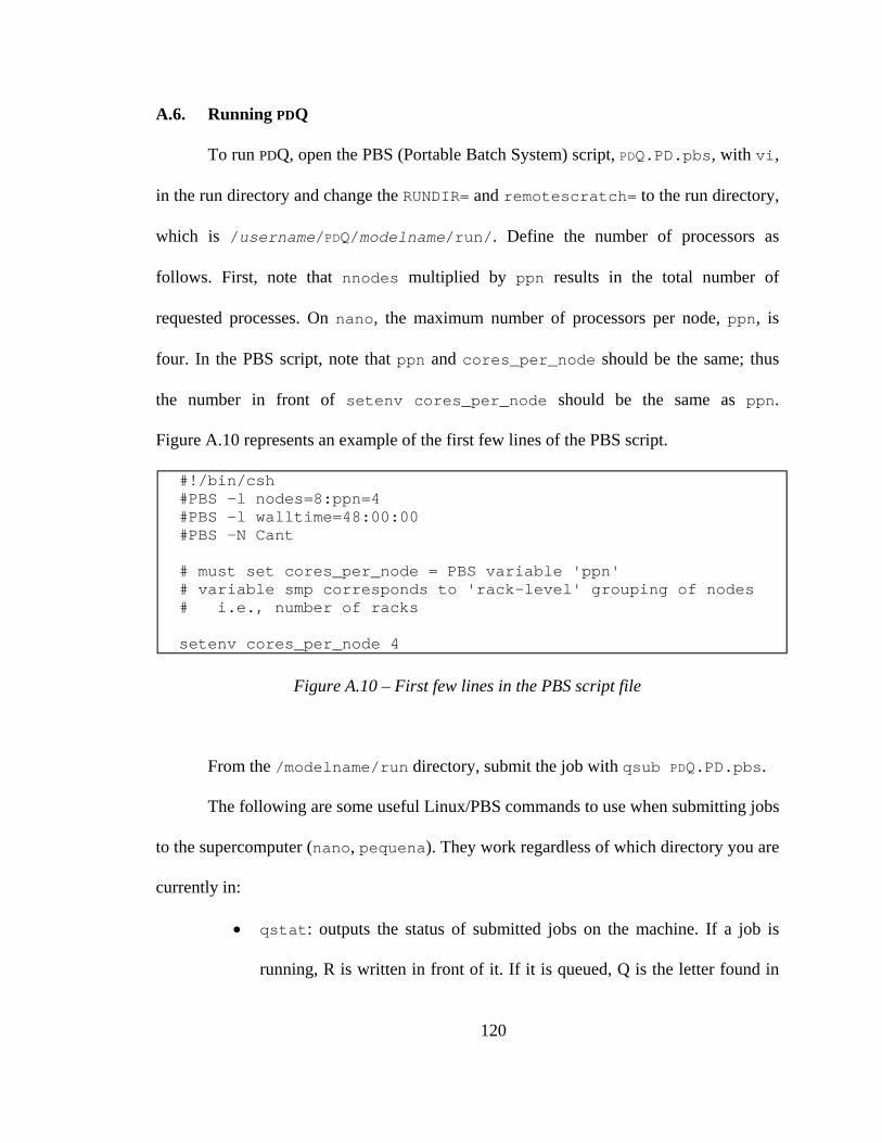
A.6. Running PDQ

To run PDQ, open the PBS (Portable Batch System) script, PDQ.PD.pbs, with vi,

in the run directory and change the RUNDIR= and remotescratch= to the run directory,

which is /username/PDQ/modelname/run/. Define the number of processors as

follows. First, note that nnodes multiplied by ppn results in the total number of

requested processes. On nano, the maximum number of processors per node, ppn, is

four. In the PBS script, note that ppn and cores_per_node should be the same; thus

the number in front of setenv cores_per_node should be the same as ppn.

Figure A.10 represents an example of the first few lines of the PBS script.

Figure A.10 – First few lines in the PBS script file

From the /modelname/run directory, submit the job with qsub PDQ.PD.pbs.

The following are some useful Linux/PBS commands to use when submitting jobs

to the supercomputer (nano, pequena). They work regardless of which directory you are

currently in:

qstat: outputs the status of submitted jobs on the machine. If a job is

running, R is written in front of it. If it is queued, Q is the letter found in

#!/bin/csh #PBS -l nodes=8:ppn=4 #PBS -l walltime=48:00:00 #PBS -N Cant # must set cores_per_node = PBS variable 'ppn' # variable smp corresponds to 'rack-level' grouping of nodes # i.e., number of racks setenv cores_per_node 4

121

front of it. You can also see more details by additional flags to the

command, for example by typing qstat –an.

qgrok: shows the number of total, occupied and free nodes.

qdel: with this command you can delete your submitted job by typing

qdel jobID, for instance qdel 12423. The jobID is integer in the first

column of the submitted job.

A.7. Post-processing

Each sample model directory has a postprocessor directory containing

Matlab files used for graphical post processing of the results.

Copy the *.dat files from /modelname/run directory to the

/modelname/postprocessor directory and run the file whose name starts with

readfiles_. Do this by typing the name of that starts with readfile_ with the time

step you want to post process as an input argument. For instance in the Matlab prompt

window type readfiles_ConcBeam(1000) for the Cant model. This will show a

deformed shape of the beam after 1000 time steps.

File “timing.o” in the run directory includes timing performance of the run. This

is a helpful file for studying the scalability and timing performance of the code. The

elapsed time and the percentage time spent on different parts of the code are tabulated in

this file.

122

REFERENCES

Allen M. P. and Tildesley D. J. (1987). Computer Simulation of Liquids, Oxford Science Publications, Oxford. Anderson T. L. (2005). Fracture Mechanics: Fundamentals and Applications, 3rd Ed., CRC Press, Boca Raton, FL. Atlas S. R., Cummings J. C., and Reynders J. V. W. (1996). “Parallel Molecular Dynamics Simulation in the POOMA FrameWork”, paper presented at the 1996 Conference on Parallel Object-Oriented Methods and Applications, Santa Fe, NM. Atlas S. R. (1999). “PDQ, a Portable, Parallel and Extensible Molecular Dynamics Simulation Program”, Technical Report, University of New Mexico. Atlas S. R. and Valone S. M. (2011). “Density Functional Theory of the Embedded-Atom Method: Multiscale Dynamical Potentials with Charge Transfer”, preprint, Physical Review B, to be submitted. Atlas S. R., Wright A. F., Ramprasad R. and Cano L. (1998-2011). “Vernet: A Parallel Planewave Pseudopotential Code for Density Functional Electronic Structure Calculations in Solids”, University of New Mexico. Barney B. (2010). “Introduction to Parallel Computing”, Lawrence Livermore National Laboratory, https://computing.llnl.gov/tutorials/parallel_comp/. Bazant Z. P. and Jirasek M. (2002). “Nonlocal Integral Formulations of Plasticity and Damage: Survey of Progress”, Journal of Engineering Mechanics, 128(11): 119-149. Beazley D. M. and Lomdahl P. S. (1994). “Message-Passing Multi-Cell Molecular Dynamics on the Connection Machine 5”, Parallel Computing, 20(2): 173-195. Bowers K. J., Chow E., Xu H., Dror R. O., Eastwood M. P., Gregersen B. A., Klepeis J. L., Kolossvary I., Moraes M. A., Sacerdoti F. D., K. Salmon, Shan Y., Shaw D. E. (2006). “Scalable Algorithms for Molecular Dynamics Simulations on Commodity Clusters”, Conference on High Performance Networking and Computing Archive, Proceedings of the 2006 ACM/IEEE Conference on Supercomputing, Tampa, Florida, Article No. 84. Bowers K., Dror R. and Shaw D. E. (2006). “The Midpoint Method for Parallelization of Particle Simulations”, Journal of Chemical Physics, 124: 184109. Bowers K., Dror R. and Shaw D. E. (2007). “Zonal methods for the parallel execution of range-limited N-body simulations”, Journal of Computational Physics, 221 (1): 303-329.

123

Brown D. and Maigret B. (1999). “Large Scale Molecular Dynamics Simulations using the Domain Decomposition Approach”, Proceedings of the 24th SPEEDUP Workshop, Berne, Sept. 24-25, 12(2): 33-41.

Bruck J., Ho C., Kipnis S. and Weathersby D. (1994). “Efficient Algorithms for All-To-All Communications in Multi-Port Message-Passing Systems”, Proceedings of the 6th Annual ACM Symposium on Parallel Algorithms and Architectures, Cape May, NJ, ACM Press, 6: 298-309.

Cusatis G., Bazant Z. P. and Cedolin L. (2006). “Confinement-Shear Lattice CSL Model for Fracture Propagation in Concrete”, Computer Methods for Applied Mechanics and Engineering, 195: 7154–7171.

Fincham D. and Ralston B. J. (1981). “Molecular Dynamics Simulation Using the Cray-1 Vector Processing Computer”, Computer Physics Communications, 23(2): 127-134.

Fincham D. (1987). “Parallel Computers and Molecular Simulation”, Molecular Simulation, 1: 1-45. Gerstle W. and Sau N. (2004). “Peridynamic Modeling of Concrete Structures”, Proceedings of the 5th Intl. Conf. on Fracture Mechanics of Concrete Structures, Li, Leung, Willam, and Billington, Eds., Ia-FRAMCOS, Vail, CO, 2: 949-956. Gerstle W., Sakhavand N. and Chapman S. (2010). “Comparison of Peridynamic and Continuum Mechanics Models for Concrete”, 7th International Conference on Fracture Mechanics of Concrete and Concrete Structures, ACI, Korea. Gerstle W. H., Sau N. and Sakhavand N. (2009). “On Peridynamic Computational Simulation of Concrete Structures”. Technical Report SP265-11, American Concrete Institute, 265: 245-264.

Gerstle W., Sau N. and Silling S. (2005). “Peridynamic Modeling of Plain and Reinforced Concrete Structures”, Proceedings of the 18th Intl. Conf. on Structural Mechanics in Reactor Technology (SMiRT 18), Atomic Energy Press, Beijing China, Aug. 7-12, 949–956.

Gerstle W. H., Sau N. and Aguilera E. (2007a). “Micropolar Modeling of Concrete Structures”, Proceedings of the 6th Intl. Conf. on Fracture Mechanics of Concrete Structures, Ia-FRAMCOS, Catania, Italy, June 17-22.

Gerstle W., Sau N. and Aguilera E. (2007b). "Micropolar Peridynamic Constitutive Model for Concrete”, 19th Intl. Conf. on Structural Mechanics in Reactor Technology (SMiRT 19), Toronto, Canada, August 12-17, B02/1-2.

124

Gerstle W., Sau N. and Silling S. (2007). “Peridynamic Modeling of Concrete Structures”, Nuclear Engineering and Design, 237(12-13): 1250-1258.

Gerstle, W., Silling, S., Read, D., Tewary, V. and Lehoucq, R. (2008). “Peridynamic Simulation of Electromigration”, Computers, Materials and Continua, Tech Science Press, 8(2): 75-92. Heffelfinger G. S. (2000). “Parallel Atomistic Simulations”, Computer Physics Communications, 128(19): 219-237.

Hendrickson B. and Plimpton S. (1992). “Parallel Many-Body Simulations Without All-To-All Communication”, Technical Report SAND92-0792, Sandia National Laboratories, Albuquerque, NM.

Hess B., Kutzner C., van der Spoel D. and Lindahl E. (2008). “GROMACS 4: Algorithms for Highly Efficient, Load-Balanced, and Scalable Molecular Simulation”, Journal of Chemical Theory and Computation, 4: 435–447.

Kadau K., Germann T. C. and Lomdahl P. S. (2006). “Molecular Dynamics Comes of Ages: 320 Bilion Atom Simulation on BlueGene/L”, Modern Physics, 17(12): 1755-1761.

LAMMPS code, (2011). Large-scale Atomic/Molecular Massively Parallel Simulator, available at [http://lammps.sandia.gov]. Lindahl E., Hess B. and van der Spoel D. (2001). “GROMACS 3.0: A Package for Molecular Simulation and Trajectory Analysis”. Journal of Molecular Modeling, 7(8): 306-317. Mase G. T., Smelser R. E. and Mase G. E. (2009). Continuum Mechanics for Engineers, 3rd Ed., CRC Press, Boca Raton, FL.

Mel'cuk A. I., Giles R. C. and Gould H. (1991). “Molecular Dynamics on the Connection Machine”. Computers in Physics 5: 311-318. Metcalf M., Reid J. and Cohen M. (2004). Fortran 95/2003 Explained (Numerical Mathematics and Scientific Computation), 3rd Ed., Oxford University Press, USA. Newton I. (1999). The Principia, 1687. See A New Translation, by Cohen I. B. and Whitman A., University of California Press, Berkeley.

Nguyen V. B., Chan A. H. C. and Crouch R. S. (2005). “Comparisons of Smeared Crack Models For RC Bridge Pier Under Cyclic Loading”, 13th ACME conference, University of Sheffield, pp. 111-114.

125

Pacheco P. S. (1998). “A User’s Guide to MPI”, Department of Mathematics, University of San Francisco, ftp://math.usfca.edu/pub/MPI/mpi.guide.ps.

Parks M. L., Lehoucq R. B., Plimpton S. J. and Silling S. A. (2008). “Implementing Peridynamics within a Molecular Dynamics Code”, Computer Physics Communications, 179: 777-783.

Phillips J. C., Braun R., Wang W., Gumbart J., Tajkhorshid E., Villa E., Chipot C., Skeel R. D., Kalé L. and Schulten K. (2005). “Scalable molecular dynamics with NAMD”, Journal of Computational Chemistry, 26(16): 1781–1802.

Plimpton S. J., (1995). “Fast Parallel Algorithms for Short-Range Molecular Dynamics”, Computational Physics, 117: 1-19. Rapaport D. C. (2004). The Art of Molecular Dynamics Simulation, 2nd Ed., Cambridge University Press, Cambridge, UK. Reynders J. V. W., Hinker P. J., Cummings J. C., Atlas S. R., Banerjee S., Humphrey W. F., Karmesin S. R., Keahey K., Srikant M., and Tholburn M. (1996). “POOMA: A Framework for Scientific Simulation on Parallel Architectures”, in: G Wilson and P Lu, eds., Parallel Programming Using C++, MIT Press, Cambridge. Runzell B., Shield C. K., French C. W. (2008). “Shear Capacity of Prestressed Concrete Beams”, Technical Report MN/RC 2007-47, Minnesota Department of Transportation, St. Paul.

Sau N. (2008). “Peridynamic Modeling of Quasi-Brittle Structures”, Ph.D. Dissertation, University of New Mexico, unpublished.

Silling S. (1998). “Reformulation of Elasticity Theory for Discontinuities and Long-Range Forces”, Technical Report SAND98-2176, Sandia National Laboratories, Albuquerque, NM.

Silling S. (2002). “Dynamic Fracture Modeling with a Meshfree Peridynamic Code”, Technical Report SAND2002-2959C, Sandia National Laboratories, Albuquerque, NM.

Silling S. A., Epton M., Weckner O., Xu J. and Askari E. (2007). “Peridynamic States and Constitutive Modeling”, Journal of Elasticity, 88: 151-184. Steinbrugge K. V. (1992). “The Earthquake Engineering Online Archive, Karl V. Steinbrugge Collection”, NISEE, University of California, Berkeley, http://nisee.berkeley.edu/elibrary/Image/S4034. The Economist (2009). “Cloud computing: Clash of the clouds”, Oct. 15th 2009.

126

Timoshenko S. P. (1983). History of Strength of Materials, Dover Publications, New York.

Valone S. M. and Atlas S. R., (2006). “Electron Correlation, Reference States, and Empirical Potentials”, Philosophical Magazine 86: 2683.

Verlet L. (1967). “Computer Experiments on Classical Fluids. I. Thermodynamical Properties of Lennard-Jones Molecules”, Yeshiva University, New York, Physical Review, 159: 98–103. Zienkiewicz O. C., Taylor R. L. (2005). The Finite Element Method for Solid and Structural Mechanics, 6th Ed., Elsevier, Oxford.

Date post:	16-Oct-2021
Category:	Documents
Upload:	others
View:	1 times
Download:	0 times

Parallel simulation of reinforced concrete sructures using ...

Documents