Parallelizing and Vectorizing Compilers

Rudolf Eigenmann and Jay Hoeflinger

January 2000

1 Introduction

Programming computers is a complex and constantlyevolving activity. Technological innovations haveconsistently increased the speed and complexity ofcomputers, making programming them more diffi-cult. To ease the programming burden, computerlanguages have been developed. A programming lan-guage employs syntactic forms that express the con-cepts of the language. Programming language con-cepts have evolved over time, as well. At first theconcepts were centered on the computing machinebeing used. Gradually, the concepts of computer lan-guages have evolved away from the machine, towardproblem-solving abstractions. Computer languagesrequire translators, called compilers, to translate pro-grams into a form that the computing machine canuse directly, called machine language.

The part of a computer that does arithmetical orlogical operations is called the processor. Processorsexecute instructions, that determine the operation toperform. An instruction that does arithmetic on oneor two numbers at a time is called a scalar instruc-tion. An instruction that operates on a larger num-ber of values at once (e.g. 32 or 64) is called a vectorinstruction. A processor that contains no vector in-structions is called a scalar processor and one thatcontains vector instructions is called a vector proces-sor. If the machine has more than one processor ofeither type, it is called a multiprocessor or a parallelcomputer.

The first computers were actually programmed byconnecting components with wires. This was a te-dious task and very error prone. If an error in thewiring was made, the programmer had to visually in-spect the wiring to find the wrong connection.

The innovation of stored-program computers elim-inated the physical wiring job. The stored-programcomputer contained a memory device that could storea series of binary digits (1s and 0s), a processingdevice that could carry out several operations, anddevices for communicating to the outside world (in-put/output devices). An instruction for this kind

of computer consisted of a numeric code indicatingwhich operation to carry out, as well as an indica-tion of the operands to which the operation was ap-plied. Debugging such a machine language programinvolved inspecting memory and finding the binarydigits that were loaded incorrectly. This could betedious and time-consuming.

Then another innovation was introduced - sym-bolic assembly language and a assembler program totranslate assembly language programs into machinelanguage. Programs could be written using namesfor memory locations and registers. This eased theprogramming burden considerably, but people stillhad to manage a group of registers, had to checkstatus bits within the processor, and keep track ofother machine-related hardware. Though the prob-lems changed somewhat, debugging was still tediousand time-consuming.

A new pair of innovations was required to lessenthe onerous attention to machine details - a new lan-guage (Fortran), closer to the domain of the prob-lems being solved, and a program for translating For-tran programs into machine code, a Fortran compiler.The 1954 Preliminary Report on Fortran stated that“. . . Fortran should virtually eliminate coding and de-bugging . . . ”.

That prediction, unfortunately, did not come true,but the Fortran compiler was an undeniable step for-ward, in that it eliminated much complexity from theprogramming process. The programmer was freedfrom managing the way machine registers were em-ployed and many other details of the machine archi-tecture.

The authors of the first Fortran compiler recog-nized that in order for Fortran to be accepted by pro-grammers, the code generated by the Fortran com-piler had to be nearly as efficient as code written inassembly language. This required sophisticated anal-ysis of the program, and optimizations to avoid un-necessary operations.

Programs written for execution by a single proces-sor are referred to as serial, or sequential programs.When the quest for increased speed produced com-

1

puters with vector instructions and multi-processors,compilers were created to convert serial programs foruse with these machines. Such compilers, called vec-torizing and parallelizing compilers, attempt to re-lieve the programmer from dealing with the machinedetails. They allow the programmer to concentrateon solving the object problem, while the compilerconcerns itself with the complexities of the machine.Much more sophisticated analysis is required of thecompiler to generate efficient machine code for thesetypes of machines.

Vector processors provide instructions that load aseries of numbers for each operand of a given opera-tion, then perform the operation on the whole series.This can be done in pipelined fashion, similar to oper-ations done by an assembly line, which is faster thandoing the operation on each item separately. Parallelprocessors offer the opportunity to do multiple oper-ations at the same time on the different processors.

This article will attempt to give the reader anoverview of the vast field of vectorizing and paral-lelizing compilers. In Section 2, we will review thearchitecture of high performance computers. In Sec-tion 3 we will cover the principle ways in which high-performance machines are programmed. In Section 4,we will delve into the analysis techniques that helpparallelizing and vectorizing compilers optimize pro-grams. In Section 5, we discuss techniques that trans-form program code in ways that can enable improvedvectorization or parallelization. Sections 6 and 7 dis-cuss the generation of vector instructions and paral-lel regions, respectively, and the issues surroundingthem. Finally, Section 9 discusses a number of im-portant compiler-internal issues.

2 Parallel Machines

2.1 Classifying Machines

Many different terms have been devised for classi-fying high performance machines. In a 1966 paper,M.J. Flynn divided computers into four classifica-tions, based on the instruction and data streams usedin the machine. These classifications have proven use-ful, and are still in use today:

1. Single instruction stream - single data stream(SISD) - these are single processor machines.

2. Single instruction stream - multiple data streams(SIMD) - these machines have two or more pro-cessors that all execute the same instruction atthe same time, but on separate data. Typically,

a SIMD machine uses a SISD machine as a host,to broadcast the instructions to be executed.

3. Multiple instruction streams - single data stream(MISD) - no whole machine of this type has everbeen built, but if it were, it would have multi-ple processors, all operating on the same data.This is similar to the idea of pipelining, wheredifferent pipeline stages operate in sequence ona single data stream.

4. Multiple instruction streams - multiple datastreams (MIMD) - these machines have two ormore processors that can all execute differentprograms and operate on their own data.

Another way to classify multiprocessor computersis according to how the programmer can think ofthe memory system. Shared-memory multiprocessors(SMPs) are machines in which any processor can ac-cess the contents of any memory location by simply is-suing its memory address. Shared-memory machinescan be thought of as having a shared memory unitaccessible to every processor. The memory unit canbe connected to the machine through a bus (a setof wires and a control unit that allows only a singledevice to connect to a single processor at one time),or an interconnection network (a collection of wiresand control units, allowing multiple data transfers atone time). If the hardware allows nearly equal accesstime to all of memory for each processor, these ma-chines can be called uniform memory access (UMA)computers.

Distributed-memory multiprocessors (DMPs) useprocessors that each have their own local memory, in-accessible to other processors. To move data from oneprocessor to another, a message containing the datamust be sent between the processors. Distributedmemory machines have frequently been called multi-computers.

Distributed shared memory (DSM) machines use acombined model, in which each processor has a sep-arate memory, but special hardware and/or softwareis used to retrieve data from the memory of anotherprocessor. Since in these machines it is faster fora processor to access data in its own memory thanto access data in another processor’s memory, thesemachines are frequently called non-uniform memoryaccess (NUMA) computers. NUMA machines maybe further divided into two categories – those inwhich cache-coherence is maintained between proces-sors (cc-NUMA) and those in which cache-coherenceis not maintained (nc-NUMA).

2

2.2 Parallel Computer Architectures

People have experimented with quite a few types ofarchitectures for high-performance computers. Therehas been a constantly re-adjusting balance betweenease of implementation and high performance.

SIMD Machines

The earliest parallel machines were SIMD machines.SIMD machines have a large number of very simpleslave processors controlled by a sequential host ormaster processor. The slave processors each contain aportion of the data for the program. The master pro-cessor executes a user’s program until it encountersa parallel instruction. At that time, the master pro-cessor broadcasts the instruction to all the slave pro-cessors, which then execute the instruction on theirdata. The master processor typically applies a bit-mask to the slave processors. If the bit-mask entryfor a particular slave processor is 0, then that pro-cessor does not execute the instruction on its data.The set of slave processors is also called an attachedarray processor because it can be built into a singleunit and attached as a performance upgrade to a uni-processor.

An early example of a SIMD machine was the IlliacIV, built at the University of Illinois during the late1960s and early 1970s. The final configuration had 64processors, one-quarter of the 256 originally planned.It was the world’s fastest computer throughout itslifetime, from 1975 to 1981. Examples of a SIMDmachine from the 1980s were the Connection Machinefrom Thinking Machines Corporation, introduced in1985, and its follow-on, the CM-2, which contained64K processors, introduced in 1987.

Vector Machines

A vector machine has a specialized instruction setwith vector operations and usually a set of vectorregisters, each of which can contain a large numberof floating point values (up to 128). With a singleinstruction, it applies an operation to all the floatingpoint numbers in a vector register. The processor ofa vector machine is typically pipelined, so that thedifferent stages of applying the operation to the vec-tor of values overlap. This also avoids the overheadsassociated with loop constructs. A scalar processorwould have to apply the operation to each data valuein a loop.

The first vector machines were the Control DataCorporation (CDC) Star-100, and the Texas Instru-ments ASC, built in the early 1970s. These machines

did not have vector registers, but rather loaded datadirectly from memory to the processor. The firstcommercially successful vector machine was the CrayResearch Cray-1. It used vector registers and paireda fast vector unit with a fast scalar unit. In the1980s, CDC built the Cyber 205 as a follow-on to theStar-100, and three Japanese companies, NEC, Hi-tachi and Fujitsu built vector machines. These threecompanies continued manufacturing vector machinesthrough the 1990s.

Shared Memory Machines

In a shared memory multi-processor, each processorcan access the value of any shared address by simplyissuing the address. Two principle hardware schemeshave been used to implement this. In the first (calledcentralized shared memory), the processors are con-nected to the shared memory via either a system busor an interconnection network. The memory bus isthe cheapest way to connect processors to make ashared memory system. However, the bus becomes abottleneck since only one device may use it at a time.An interconnection network has more inherent paral-lelism, but involves more expensive hardware. In thesecond (called distributed shared-memory), each pro-cessor has a local memory, and whenever a processorissues the address of a memory location not in its lo-cal memory, special hardware is activated to fetch thevalue from the remote memory that contains it.

The Sperry Rand 1108 was an early centralizedshared memory computer, built in the mid 1960s.It could be configured with up to three processorsplus two input/output controller processors. In the1970s, Carnegie Mellon University built the C.mmpas a research machine, connecting 16 minicomput-ers (PDP-11s) to 16 memory units through a cross-bar interconnection network. Several companies builtbus-based centralized shared memory computers dur-ing the 1980s, including Alliant, Convex, Sequent andEncore. The 1990s saw fewer machines of this typeintroduced. A prominent manufacturer was SiliconGraphics Inc. (SGI), which produced the Challengeand Power Challenge systems in that period.

During the 1980s and 1990s, several research ma-chines explored the distributed shared memory archi-tecture. The Cedar machine built at the Universityof Illinois in the late 1980s connected a number ofbus-based multiprocessors (called clusters) with aninterconnection network to a global memory. Theglobal memory modules contained special synchro-nization processors which allowed clusters to syn-chronize. The Stanford DASH, built in the early1990s, also employed a two-level architecture, but

3

added a cache-coherence mechanism. One node ofthe DASH was a bus-based multiprocessor with a lo-cal memory. A collection of these nodes were con-nected together in a mesh. When a processor referredto a memory location not contained within the localnode, the node’s directory was consulted to determinethe remote location. The MIT Alewife project alsoproduced a directory-based machine. A prominentdirectory-based commercial machine was the Origin2000 from SGI.

Distributed Memory Multiprocessors

In a distributed memory multiprocessor, each proces-sor has access to its local memory only. It can onlyaccess values from a different memory by receivingthem in a message from the processor whose memorycontains them. The other processor must be pro-grammed to send the value at the right time.

People started extensive experimentation withDMPs in the 1980s. They were searching for waysto construct computers with large numbers of pro-cessors cheaply. Bus-based machines were easy tobuild, but suffered from a limitation on bus commu-nications bandwidth, and were hampered by the se-rialization required to use the bus. Machines builtusing interconnection networks or cross-bar switcheshad increased bandwidth and communication paral-lelism, but were expensive to build. Multicomput-ers simply connected processor/memory nodes withcommunication lines in a number of configurations,from meshes to toroids to hypercubes. These turnedout to be cheap to build and (usually) had sufficientmemory bandwidth. The principle drawback of thesemachines was the difficulty of writing programs forthem.

One example of a DMP in the 1980s was a Hyper-cube research machine built at the California Insti-tute of Technology, which had processors connectedin a hypercube topology by communication links.The nCUBE company and Intel Scientific Computerswere founded to build similar machines. nCUBE builtthe nCUBE/1 and nCUBE/2, while ISC built theiPSC/1 and iPSC/2. In the 1990s, nCUBE followedwith the nCUBE/2S, and ISC built the iPSC/860,the iWarp for Carnegie Mellon University and theParagon.

COMA

A machine that uses all of its memory as a cacheis called a cache-only memory architecture (COMA).Typically in these machines, each processor has a lo-cal memory, and data is allowed to move from one

processor’s memory to another during the run of aprogram. The term attraction memory has been usedto describe the tendency of data to migrate towardthe processor that uses it the most. Theoretically,this can minimize the latency to access data, sincelatency increases as the data get further from theprocessor.

The COMA idea was introduced by a team at theSwedish Institute of Computer Science, working onthe Data Diffusion Machine. The idea was commer-cialized by Kendall Square Research (KSR), whichbuilt the KSR1 in the early 1990s.

Multi-threaded Machines

A multi-threaded machine attempts to hide latencyto memory by overlapping it with computation. Assoon as the processor is forced to wait for a dataaccess, it switches to another thread to do more com-putation. If there are enough threads to keep theprocessor busy until each piece of data arrives, thenthe processor is never idle.

The Denelcor HEP machine was the first multi-threaded processor in the early 1980s. In the 1990s,the Alewife machine used multi-threading in the pro-cessor to help hide some of the latency of memoryaccesses. Also, in the 90s, the Tera Computer Com-pany developed the MTA machine, which expandedon many of the ideas used in the HEP.

Clusters of SMPs

Another approach to building a multiprocessor is touse a small number of commodity microprocessors tomake centralized shared-memory clusters, then con-nect large numbers of these together. The numberof microprocessors to use to make a single clusterwould be determined by the number of processorsthat would saturate the bus (keep the bus constantlybusy). Such machines are called clusters of SMPs.Clusters of SMPs have the advantage of being cheapto build. During the second half of the 1990s, peoplebegan building clusters out of low-cost components:Pentium processors, a fast network (such as Ether-net or Myrinet), the Linux operating system, and theMessage Passing Interface (MPI) library. These ma-chines are sometimes referred to as Beowulf clusters.

3 Programming Parallel Ma-chines

From a user’s point of view there are three differentways of creating a parallel program:

4

1. writing a serial program and compiling it with aparallelizing compiler

2. composing a program from modules that havealready been implemented as parallel programs

3. writing a program that expresses parallel activi-ties explicitly

Option 1 above is obviously the easiest for the pro-grammer. It is easier to write a serial program thanit is to write a parallel program. The programmerwould write the program in one of the languages forwhich a parallelizing compiler is available (Fortran,C, and C++), then employ the compiler. The tech-nology that supports this scenario is the main focusof this article.

Option 2 above can be easy as well, because theuser does not need to deal with explicit parallelism.For many problems and computer systems there existlibraries that perform common operations in parallel.Among them, mathematical libraries for manipulat-ing matrices are best known. One difficulty for usersis that one must make sure that a large fraction ofthe program execution is spent inside such libraries.Otherwise, the serial part of the program may domi-nate the execution time when running the applicationon many processors.

Option 3 above is the most difficult for program-mers, but gives them direct control over the perfor-mance of the parallel execution. Explicit parallel lan-guages are also important as a target for parallelizingcompilers. Many parallelizers act as source-to-sourcerestructurers, translating the original, serial programinto parallel form. The actual generation of paral-lel code is then performed by a “backend compiler”from this parallel language form. The remainder ofthis section discusses this option in more detail.

Expressing Parallel Programs

Syntactically, parallel programs can be expressed invarious ways. A large number of languages offer par-allel programming constructs. Examples are Prolog,Haskell, Sisal, Multilisp, Concurrent Pascal, Occamand many others. Compared to standard, sequentiallanguages they tend to be more complex, available onless machines, and lack good debugging tools, whichcontributes to the degree difficulty facing the user ofOption 3 above.

Parallelism can also be expressed in the form ofdirectives, which are pseudo comments with seman-tics understood by the compiler. Many manufac-turers have devised their own set of such directives(Cray, SGI, Convex, etc.), but during the 1990s the

OpenMP standard emerged. OpenMP describes acommon set of directives for implementing varioustypes of parallel execution and synchronization. Oneadvantage of the OpenMP directives is that they aredesigned to be added to a working serial code. If thecompiler is told to ignore the directives, the serialprogram will still execute correctly. Since the serialprogram is unchanged, such a parallel program maybe easier to debug.

A third way of expressing parallelism is to use li-brary calls within an otherwise sequential program.The libraries perform the task of creating and termi-nating parallel activities, scheduling them, and sup-porting communication and synchronization. Exam-ples of libraries that support this method are thePOSIX threads package, which is supported by manyoperating systems, and the MPI libraries, which havebecome a standard for expressing message passingparallel applications.

Parallel Programming Models

Programming Vector Machines: Vector paral-lelism typically exploits operations that are per-formed on array data structures. This can be ex-pressed using vector constructs that have been addedto standard languages. For instance, Fortran90 usesconstructs such as

A(1:n) = B(1:n) + C(1:n)

For a vector machine, this could cause a vector loopto be produced, which performs a vector add betweenchunks of arrays B and C, then a vector copy of theresult into a chunk of array A. The size of a chunkwould be determined by the number of elements thatfit into a vector register in the machine.

Loop Parallelism: Loops express repetitive exe-cution patterns, which is where most of a program’swork is performed. Parallelism is exploited by iden-tifying loops that have independent iterations. Thatis, all iterations access separate data. Loop paral-lelism is often expressed through directives, whichare placed before the first statement of the loop.OpenMP is an important example of a loop-orienteddirective language. Typically, a single processor exe-cutes code between loops, but activates (forks) a setof processors to cooperate in executing the parallelloop. Every processor will execute a share of theloop iterations. A synchronization point (or barrier)is typically placed after the loop. When all proces-sors arrive at the barrier, only the master processorcontinues. This is called a join point for the loop.

5

Thus the term fork/join parallelism is used for loopparallelism.

Determining which processor executes which iter-ation of the loop is called scheduling. Loops maybe scheduled statically, which means that the assign-ment of processors to loop iterations is fully deter-mined prior to the execution of the loop. Loops mayalso be self-scheduled, which means that whenever agiven processor is ready to execute a loop iteration, ittakes the next available iteration. Other schedulingtechniques will be discussed in Section 7.3.

Parallel Threads Model: If the parallel activi-ties in a program can be packaged well in the form ofsubroutines that can execute independently of eachother, then the threads model is adequate. Threadsare parallel activities that are created and terminatedexplicitly by the program. The code executed by athread is a specified subroutine, and the data accessedcan either be private to a thread or shared with otherthreads. Various synchronization constructs are usu-ally supported for coordinating parallel threads. Us-ing the threads model, users can implement highlydynamic and flexible parallel execution schemes. ThePOSIX threads package is one example of a well-known library that supports this model.

The SPMD Model: Distributed-memory paral-lel machines are typically programmed by using theSPMD execution model. SPMD stands for “singleprogram, multiple data”. This refers to the fact thateach processor executes an identical program, but ondifferent data. One processor can not directly accessthe data of another processor, but a message contain-ing that data can be passed from one processor to theother. The MPI standard defines an important formfor passing such messages. In a DMP, a processor’saccess to its own data is much faster than access todata of another processor through a message, so pro-grammers typically write SPMD programs that avoidaccess to the data of other processors. Programs writ-ten for a DMP can be more difficult to write thanprograms written for an SMP, because the program-mer must be much more careful about how the datais accessed.

4 Program Analysis

Program analysis is crucial for any optimizing com-piler. The compiler writer must determine the analy-sis techniques to use in the compiler based on the tar-get machine and the type of optimization desired. For

parallelization and vectorization, the compiler typi-cally takes as input the serial form of a program, thendetermines which parts of the program can be trans-formed into parallel or vector form. The key con-straint is that the “results” of each section of codemust be the same as those of the serial program.Sometimes the compiler can parallelize a section ofcode in such a way that the order of operations isdifferent than that in the serial program, causing aslightly different result. The difference may be sosmall as to be unimportant, or actually might alterthe results in an important way. In these cases, theprogrammer must agree to let the compiler parallelizethe code in this manner.

Some of the analysis techniques used by paralleliz-ing compilers are also done by optimizing compilerscompiling for serial machines. In this section we willgenerally ignore such techniques, and focus on thetechniques that are unique to parallelizing and vec-torizing compilers.

4.1 Dependence Analysis

A data dependence between two sections of a pro-gram indicates that during execution of the optimizedprogram, those two sections of code must be run inthe order indicated by the dependence. Data depen-dences between two sections of code that access thesame memory location are classified based on the typeof the access (read or write) and the order, so thereare four classifications:

input dependence: READ before READ

anti dependence: READ before WRITE

flow dependence: WRITE before READ

output dependence: WRITE before WRITE

Flow dependences are also referred to as true de-pendences. If an input dependence occurs betweentwo sections of a program, it does not prevent thesections from running at the same time (in parallel).However, the existence of any of the other types ofdependences would prevent the sections from run-ning in parallel, because the results may be differ-ent from those of the serial code. Techniques havebeen developed for changing the original program inmany situations where dependences exist, so that thesections can run in parallel. Some of them will bedescribed later in this article.

A loop is parallelized by running its iterations inparallel, so the question must be asked whether thesame storage location would be accessed in different

6

iterations of a loop, and whether one of the accesses isa write. If so, then a data dependence exists withinthe loop. Data dependence within a loop is typi-cally determined by equating the subscript expres-sions of each pair of references to a given array, andattempting to solve the equation (called the depen-dence equation), subject to constraints imposed bythe loop bounds. For a multi-dimensional array, thereis one dependence equation for each dimension. Thedependence equations form a system of equations, thedependence system, which is solved simultaneously. Ifthe compiler can find a solution to the system, or if itcannot prove that there is no solution, then it mustconservatively assume that there is a solution, whichwould mean that a dependence exists. Mathematicalmethods for solving such systems are well known ifthe equations are linear. That means, the form of thesubscript expressions is as follows:

k∑j=1

ajij + a0

where k is the number of loops nested around an arrayreference, ij is the loop index in the jth loop in thenest, and aj is the coefficient of the jth loop index inthe expression.

The dependence equation would be of the form:

k∑j=1

aji′j + a0 =

k∑j=1

bji′′j + b0 (1)

or

k∑j=1

(aji′j − bji

′′j ) = b0 − a0 (2)

In these equations, i′j and i′′j represent the values

of the jth loop index of the two subscript expressionsbeing equated. For instance, consider the loop below.

DO i = 1, 100A(i) = B(i)C(i) = A(i-1)

ENDDO

There are two references to array A, so we equatethe subscript expressions of the two references. Theequation would be:

i′1 = i′′1 − 1

subject to the constraints:

i′1 < i′′1

1 ≤ i′1 ≤ 100

1 ≤ i′′1 ≤ 100

The constraint i′1 < i′′1 comes from the idea thatonly dependences across iterations are important. Adependence within the same iteration (i′1 ≡ i′′1) isnever a problem, since each iteration executes on asingle processor, so it can be ignored.

Of course, there are many solutions to this equationthat satisfy the constraints: {i′1 : 1, i′′1 : 2} is one;{i′1 : 2, i′′1 : 3} is another. Therefore, the given loopcontains a dependence.

A dependence test is an algorithm employed to de-termine if a dependence exists in a section of code.The problem of finding dependence in this way hasbeen shown to be equivalent to the problem of find-ing solutions to a system of Diophantine equations,which is NP-complete, meaning that only extremelyexpensive algorithms can be found to solve the com-plete problem exactly. Therefore, a large number ofdependence tests have been devised that solve theproblem under simplifying conditions and in specialsituations.

Iteration Spaces

Looping statements with pre-evaluated loop bounds,such as the Fortran do-loop, have a predetermined setof values for their loop indices. This set of loop-indexvalues is the iteration space of the loop. k-nested loopstatements have a k-dimensional iteration space. Aspecific iteration within that space may be namedby a k-tuple of iteration values, called an iterationvector:

{i1, i2, · · · , ik}

in which i1 represents the outermost loop, i2 the nextinner, and ik is the innermost loop.

Direction and Distance Vectors

When a dependence is found in a loop nest, it is some-times useful to characterize it by indicating the itera-tion vectors of the iterations where the same locationis referenced. For instance, consider the followingloop.

DO i = 2, 100DO j = 1, 100

S1: A(i,j) = B(i)S2: C(i) = A(i-1,j+3)

ENDDOENDDO

7

The dependence between statements S1 and S2happens between iterations

{2, 5} and {3, 2}, {2, 6} and {3, 3}, etc

Since {2, 5} happens before {3, 2} in the serial ex-ecution of the loop nest, we say that the dependencesource is {2, 5} and the dependence sink is {3, 2}. Thedependence distance for a particular dependence is de-fined as the difference between the iteration vectors,the sink minus the source.

dependence distance = {3, 2} − {2, 5} = {1,−3}

Notice that in this example the dependence dis-tance is constant, but this may not always be thecase.

The dependence direction vector is also useful in-formation, though coarser than the dependence dis-tance. There are three directions for a dependence:{<,=, >}. The < direction corresponds to a positivedependence distance, the = direction corresponds toa distance of zero, and the > direction corresponds toa negative dependence distance. Therefore, the direc-tion vector for the example above would be {<,>}.

Distance and direction vectors are used within par-allelizing compilers to help determine the legality ofvarious transformations, and to improve the efficiencyof the compiler. Loop transformations that reorderthe iteration space, or modify the subscripts of arrayreferences within loops cannot be applied for someconfigurations of direction vectors. In addition, inmultiply-nested loops that refer to multi-dimensionalarrays, we can hierarchically test for dependence,guided by the direction vectors, and thereby makefewer dependence tests. Distance vectors can helppartially parallelize loops, even in the presence of de-pendences.

Exact versus Inexact Tests

There are three possible answers that any dependencetest can give:

1. No dependence - the compiler can prove that nodependence exists.

2. Dependence - the compiler can prove that a de-pendence exists.

3. Not sure - the test could neither prove nor dis-prove dependences. To be safe, the compilermust assume a dependence in this case. This isthe conservative assumption for dependence test-ing, necessary to guarantee correct execution ofthe parallel program.

We call a dependence test exact if it only reportsanswers 1 or 2. Otherwise, it is inexact.

Dependence Tests

The first of the dependence tests was the GCD test,an inexact test. The GCD test finds the greatest com-mon divisor g of the coefficients of the left-hand-sideof the dependence equation (Equation 2 above). Ifg does not divide the right-hand-side value of Equa-tion 2, then there can be no dependence. Otherwise,a dependence is still a possibility. The GCD test ischeap compared to some other dependence tests. Inpractice, however, often the GCD g is 1, which willalways divide the right-hand-side, so the GCD testdoesn’t help in those cases.

The Extreme Value test, also inexact in the generalcase, has proven to be one of the most useful depen-dence tests. It takes the dependence equation (2) andconstructs both the minimum and the maximum pos-sible values for the left-hand-side. If it can show thatthe right-hand-side is either greater than the maxi-mum, or less than the minimum, then we know forcertain that no dependence exists. Otherwise, a de-pendence must be assumed. A combination of theExtreme Value test and the GCD test has proved tobe very valuable and fast because they complementeach other very well. The GCD test does not in-corporate information about the loop bounds, whichthe Extreme Value test provides. At the same time,the Extreme Value test does not concern itself withthe structure of the subscript expressions, which theGCD test does.

The Extreme Value test is exact under certain con-ditions. It is exact if any of the following are true:

• all loop index coefficients are ±1 or 0,

• the coefficient of one index variable is ±1 andthe magnitudes of all other coefficients are lessthan the range of that index variable, or

• the coefficient of one index variable is ±1 andthere exists a permutation of the remaining in-dex variables such that the coefficient of eachis less than the sum of the products of the co-efficients and ranges for all the previous indexvariables.

Many other dependence tests have been devisedover the years. Many deal with ways of solving thedependence system when it takes certain forms. Forinstance, the Two Variable Exact test can find anexact solution if the dependence system is a singleequation of the form:

8

ai+ bj = c

.The most general dependence test would be to use

integer programming to solve a linear system - a setof equations (the dependence system) and a set of in-equalities (constraints on variables due to the struc-ture of the program). Integer programming conductsa search for a set of integer values for the variablesthat satisfy the linear system. Fourier-Motzkin elim-ination is one algorithm that is used to conduct thesearch for solutions. Its complexity is very high (ex-ponential), so until the advent of the Omega test (dis-cussed below), it was considered too expensive to useinteger programming as a dependence test.

The Lambda test is an increased-precision form ofthe Extreme Value test. While the Extreme Valuetest basically checks to see whether the hyper-planeformed by any of the dependence equations falls com-pletely outside the multi-dimensional volume delim-ited by the loop bounds of the loop nest in question,the Lambda test checks for the situation in whicheach hyper-plane intersects the volume, but the in-tersection of all hyper-planes falls outside the volume.It is especially useful for the situation in which a sin-gle loop index appears in the subscript expressionfor more than one dimension of an array reference(a reference referred to as having coupled subscripts).If the Lambda test can find that the intersection ofany two dependence equation hyper-planes falls com-pletely outside the volume, then it can declare thatthere is no solution to the dependence system.

The I Test is a combination of the GCD and Ex-treme Value tests, but is more precise than would bethe application of the two tests individually.

The Generalized GCD test, built on GaussianElimination (adapted for integers) attempts to solvethe system of dependence equations simultaneously.It forms a matrix representation of the dependencesystem, then using elementary row operations formsa solution of the dependence system, if one exists.The solution is parameterized so that all possible so-lutions could be generated. The dependence distancecan also be determined by this method.

The Power Test first uses the Generalized GCDtest. If that produces a parameterized solution tothe dependence system, then it uses constraints de-rived from the program to determine lower and upperbounds on the free variables of the parameterized so-lution. Fourier-Motzkin elimination is used to com-bine the constraints of the program for this purpose.These extra constraints can sometimes produce an

impossible result, indicating that the original param-eterized solution was actually empty, disproving thedependence. The Power Test can also be used to testfor dependence for specific direction vectors.

All of the preceding dependence tests are applica-ble when all coefficients and loop bounds are integerconstants and the subscript expressions are all affinefunctions. The Power Test is the only test mentionedup to this point that can make use of variables ascoefficients or loop bounds. A variable can simply betreated as an additional unknown. The value of thevariable would simply be expressed in terms of thefree variables of the solution, then Fourier-Motzkinelimination could incorporate any constraints on thatvariable into the constraints on the free variables ofthe solution. A small number of dependence testshave been devised that can make use of variables andnon-affine subscript expressions.

The Omega test makes use of a fast algorithm fordoing Fourier-Motzkin elimination. The original de-pendence problem that it tries to solve consists of aset of equalities (the dependence system), and a set ofinequalities (the program constraints). First, it elimi-nates all equality constraints (as was done in the Gen-

eralized GCD test) by using a specially-designed m̂odfunction to reduce the magnitude of the coefficients,until at least one reaches ±1, when it is possible toremove the equality. Then, the set of resulting in-equalities is tested to determine whether any integersolutions can be found for them. It has been shownthat, for most real program situations, the Omegatest gives an answer quickly (polynomial time). Insome cases, however, it cannot and it resorts to anexponential-time search.

The Range test extends the Extreme Value test tosymbolic and nonlinear subscript expressions. Theranges of array locations accessed by adjacent loopiterations are symbolically compared. The Range testmakes use of range information for variables withinthe program, obtained by symbolically analyzing theprogram. It is able to discern data dependences ina few, important situations that other tests cannothandle.

The recent Access Region test makes use of a sym-bolic representation of the array elements accessed atseparate sites within a loop. It uses an intersectionoperation to intersect two of these symbolic access re-gions. If the intersection can be proven empty, thenthe potential dependence is disproven. The AccessRegion test likewise can test dependence when non-affine subscript expressions are used, because in somecases it can apply simplification operators to expressthe regions in affine terms.

9

An array subscript expression classification systemcan assist dependence testing. Subscript expressionsmay be classified according to their structure, thenthe dependence solution technique may be chosenbased on how the subscript expressions involved areclassified. A useful classification of the subscript ex-pression pairs involved in a dependence problem is asfollows:

ZIV (zero index variable) The two subscript ex-pressions contain no index variables at all, e.g.A(1) and A(2).

SIV (single index variable) The two subscript ex-pressions contain only one loop index variable,e.g. A(i) and A(i+2).

MIV (multiple index variable) The two subscriptexpressions contain more than one loop indexvariable, e.g. A(i) and A(j) or A(i+j) andA(i).

The different classifications call for unique depen-dence testing methods. The SIV class is further sub-divided into various special cases, each enabling aspecial dependence test or loop transformation.

The Delta test makes use of these subscript ex-pression classes. It first classifies each dependenceproblem according to the above types. Then, it usesa specially-targeted dependence test for each case.The main insight of the Delta test is that when twoarray references are being tested for dependence, in-formation derived from solving the dependence equa-tion for one dimension may be used in solving thedependence equation for another dimension. This al-lows the Delta test to be useful even in the presenceof coupled subscripts. The algorithm attends to theSIV and ZIV equations first, since they can be solvedeasily. Then, the information gained is used in thesolution of the MIV equations. Since the Delta testdoes not attempt to use a single general techniqueto determine dependence, but rather special tests foreach special case, it is possible for the Delta test toaccommodate unknown variable values more easily.

Run-time Dependence Testing

It is very common for programs to make heavy use ofvariables whose values are read from input files. Un-fortunately, such variables often contain crucial in-formation about the dependence pattern of the pro-gram. In this type of situation, a perfectly parallelloop might have to be run serially, simply becausethe compiler lacked information about the input vari-ables. In these cases, it is sometimes possible for

the compiler to compile a test into the program thatwould test for certain parallelism-enabling conditions,then choose between parallel and serial code based onthe result of the test. This technique of paralleliza-tion is called run-time dependence testing.

The inspector/executor model of program execu-tion allows a compiler to run some kind of analysis ofthe data values in the program (the inspector), whichsets up the execution, then to execute the code basedon the analysis (the executor). The inspector cando anything from dependence testing to setting up acommunication pattern to be carried out by the ex-ecutor. The complexity of the test needed at run-timevaries based on the details of the loop itself. Some-times the test needed is very simple. For instance, inthe loop

DO i=1,100A(i+m) = B(i)C(i) = A(i)

ENDDO

no dependence exists in the loop if m > 99. Thecompiler might generate code that executes a paral-lel version of the loop if m > 99, otherwise a serialversion.

More complicated situations might call for a moresophisticated dependence test to be performed at run-time. The compiler might be able to prove all con-ditions for independence except one. Proof of thatcondition might be attempted at run-time. For ex-ample, the compiler might determine that a loop isparallel if only a given array was proven to containno duplicate values (i.e. be a permutation vector).If the body of the loop is large enough, then thetime savings of running the loop in parallel can besubstantial. It could offset the expense of checkingfor the permutation vector condition at runtime. Inthis case, the compiler might generate such a test tochoose between the serial and parallel versions of theloop.

Another technique that has been employed is toattempt to run a loop in parallel despite not know-ing for sure that the loop is parallel. This is calledspeculative parallelization. The pre-loop values of thememory locations that will be modified by the loopmust be saved because it might be determined dur-ing execution that the loop contained a dependence,in which case the results of the parallel run must bediscarded and the loop must be re-executed serially.During the parallel execution of the loop, extra codeis executed that can be used to determine whether adependence really did exist in the serial version. The

10

LRPD test is one example of such a runtime depen-dence test.

4.2 Interprocedural Analysis

A loop containing one or more procedure callspresents a special challenge for parallelizing compil-ers. The chief problem is how to compare the memoryactivity in different execution contexts (subroutines),for the purpose of discovering data dependences. Onepossibility, called subroutine inlining, is to remove allsubroutine calls by directly replacing all subroutinecalls with the code from the called subroutine, thenparallelizing the whole program as one large routine.This is sometimes feasible, but often causes an explo-sion in the amount of source code that the compilermust compile. Inlining also faces obstacles in tryingto represent the formal parameters of the subroutinein the context of the calling routine, since in some lan-guages (Fortran is one example) it is legal to declareformal parameter arrays with dimensionality differentfrom that in the calling routine.

The alternative to inlining is to keep the subroutinecall structure intact and simply represent the memoryaccess activity caused by a subroutine in some way atthe call site. One method of doing this is to representmemory activity symbolically with sets of constraints.For instance, at the site of a subroutine call, it mightbe noted that the locations written were:

{A(i) | 0 ≤ i ≤ 100}

The advantage of using this method is that one canuse the sets of constraints directly with a Fourier-Motzkin-based dependence test.

Several other forms for representing memory ac-cesses have been used in various compilers. Many arebased on triplet notation, which represents a set ofmemory locations in the form:

lower bound : upper bound : stride

This form can represent many regular access pat-terns, but not all.

Another representational form consists of RegularSection Descriptors (RSDs), which uses a simple form(I+α), where I is a loop index and α is a loop invari-ant expression. At least three other forms based onRSDs have been used: Restricted RSDs (which canexpress access on the diagonal of an array), BoundedRSDs that express triplet notation with full symbolicexpressions, and Guarded Array Regions, which areBounded RSDs qualified with a predicate guard.

An alternative for representing memory activity in-terprocedurally is to use a representational format

whose dimensionality is not tied to the program-declared dimensionality of a given array. An exampleof this type is the Linear Memory Access Descriptorsused in the Access Region test. This form can repre-sent most memory access patterns used in a program,and allows one to represent memory reference activityconsistently across procedure boundaries.

4.3 Symbolic Analysis

Symbolic analysis refers to the use of symbolic termswithin ordinary compiler analysis. The extent towhich a compiler’s analysis can handle expressionscontaining variables is a measure of how good a com-piler’s symbolic analysis is. Some compilers use anintegrated, custom-built symbolic analysis package,which can apply algebraic simplifications to expres-sions. Others depend on integrated packages, suchas the Omega constraint-solver, to do the symbolicmanipulation that they need. Still others use linksto external symbolic manipulation packages, such asMathematica or Maple. Modern parallelizing compil-ers generally have sophisticated symbolic analysis.

4.4 Abstract Interpretation

When compilers need to know the result of executinga section of code, they often traverse the programin “execution order”, keeping track of the effect ofeach statement. This process is called abstract inter-pretation. Since the compiler generally will not haveaccess to the runtime values of all the variables in theprogram, the effect of each statement will have to becomputed symbolically. The effect of a loop is easilydetermined when there is a fixed number of iterations(such as in a Fortran do-loop). For loops that donot explicitly state a number of iterations, the effectof the iteration may be determined by widening, inwhich the values changing due to the loop are made tochange as though the loop had an infinite number ofiterations, and then narrowing, in which an attemptis made to factor in the loop exit conditions, to limitthe changes due to widening. Abstract interpretationfollows all control flow paths in the program.

Range Analysis Range analysis is an applicationof abstract interpretation. It gathers the range ofvalues that each variable can assume at each point inthe program. The ranges gathered have been used tosupport the Range test, as mentioned in Section 4.1above.

11

4.5 Data Flow Analysis

Many analysis techniques need global informationabout the program being compiled. A general frame-work for gathering this information is called data flowanalysis. To use data flow analysis, the compilerwriter must set up and solve systems of data flowequations that relate information at various points ina program. The whole program is traversed and in-formation is gathered from each program node, thenused in the data flow equations. The traversal of theprogram can be either forward (in the same directionas normal execution would proceed), or backward (inthe opposite direction from normal execution). Atjoin points in the program’s control flow graph, theinformation coming from the paths that join must becombined, so the rules which govern that combinationmust be specified.

The data flow process proceeds in the direc-tion specified, gathering the information by solvingthe data flow equations, and combining informationat control flow join points until a steady-state isachieved. That is, until no more changes occur inthe information being calculated. When steady stateis achieved, the wanted information has been propa-gated to each point in the program.

An example of data flow analysis is constant prop-agation. By knowing the value of a variable at a cer-tain point in the program, the precision of compileranalysis can be improved. Constant propagation isa forward data flow problem. A value is propagatedfor each variable. The value gets set whenever anassignment statement in the program assigns a con-stant to the variable. The value remains associatedwith the variable until another assignment statementassigns a value to the variable. At control flow joinpoints in the program, if a value is associated with thevariable on all incoming paths, and it is always thesame value, then that value stays associated with thevariable. Otherwise, the value is set to “unknown”.

Data flow analysis can be used for many purposeswithin a compiler. It can be used for determiningwhich variables are aliased to which other variables,for determining which variables are potentially modi-fied by a given section of code, for determining whichvariables may be pointed to by a given pointer, andmany other purposes. Its use generally increases theprecision of other compiler analyses.

4.6 Code Transformations to AidAnalysis

Sometimes program source code can be transformedin a way that encodes useful information about the

program. The program can be translated into a re-stricted form that eliminates some of the complexi-ties of the original program. Two examples of thisare control-flow normalization and Static Single As-signment (SSA) form.

Control-flow normalization is applied to a programto transform it to a form that is simpler to analyzethan a program with arbitrary control flow. An ex-ample of this is the removal of GOTO statements from aFortran program, replacing them with IF statementsand looping constructs. This adds information to theprogram structure, which can be used by the compilerto possibly do a better job of optimizing the program.

Another example is to transform a program intoSSA form. In SSA form, each variable is assigned ex-actly once and is only read thereafter. When a vari-able in the original program is assigned more thanonce, it is broken into multiple variables, each ofwhich is assigned once. SSA form has the advan-tage that whenever a given variable is used, there isonly one possible place where it was assigned, so moreprecise information about the value of the variable isencoded directly into the program form.

Gated SSA form Gated SSA form is a variant ofSSA form that includes special conditional expres-sions (gating expressions) that make the representa-tion more precise. Gated SSA form has been usedfor flow-sensitive array privatization analysis withina loop. Array privatization analysis requires that thecompiler prove that writes to a portion of an array beshown to precede all reads to the same section of thearray within the loop. When conditional branchinghappens within the loop, then the gating expressionscan help to prove the privatization condition.

5 Enabling Transformations

Like all optimizing compilers, parallelizers and vec-torizers consist of a sequence of compilation passes.The program analysis techniques described so far areusually the first set of these passes. They gather in-formation about the source program, which is thenused by the transformation passes to make intelli-gent decisions. The compilers have to decide whichtransformations can legally and profitably be appliedto which code sections and how to best orchestratethese transformations.

For the sake of this description we divide the trans-formations into two parts, those that enable othertechniques and those that perform the actual vector-izing or parallelizing transformations. This division

12

is useful for our presentation, but not strict. Sometechniques will be mentioned in both places.

5.1 Dependence Elimination andAvoidance

An important class of enabling transformations dealswith eliminating and avoiding data dependences. Wewill describe data privatization, idiom recognition,and dependence-aware work partitioning techniques.

Data Privatization and Expansion

Data privatization is one of the most important tech-niques because it directly enables parallelization andit applies very widely. Data privatization can re-move anti and output dependences. These so-calledstorage-related or false dependences are not due tocomputation having to wait for data values producedby another computation. Instead, the computationmust wait because it wants to assign a value to avariable that is still in use by a previous computa-tion. The basic idea is to use a new storage locationso that the new assignment does not overwrite theold value too soon. Data privatization does this asshown in Figure 1.

Figure 1: Data Privatization and Expansion.

In the original code, each loop iteration uses thevariable t as a temporary storage. This representsa dependence, in that each iteration would have towait until the previous iteration is done using t. Inthe sequential execution of the program this orderis guaranteed. However, in a parallel execution wewould like to execute all iterations concurrently ondifferent processors. The transformed code simplymarks t as a privatizable variable. This instructs thecode-generating compiler pass to place t into the pri-vate storage of each processor - essentially p timesreplicating the variable t, where p is the number of

processors. Data expansion is an alternative imple-mentation to privatization. Instead of marking t pri-vate, the compiler expands the scalar variable into anarray and uses the loop variable as an array index.

The main difficulty of data privatization and ex-pansion is to recognize eligible variables. A variableis privatizable in a loop iteration if it is assigned be-fore it is used. This is relatively simple to detect forscalar variables. However, the transformation is im-portant for arrays as well. The analysis of array sec-tions that are provably assigned before used can bevery involved and requires symbolic analysis, men-tioned in Section 4.

Idiom Recognition: Reductions, Inductions,Recurrences

These transformations can remove true (i.e., flow) de-pendences. The elimination of situations where onecomputation has to wait for another to produce aneeded data value, is only possible if we can expressthe computation in a different way. Hence, the com-piler recognizes certain idioms and rewrites them ina form that exhibits more parallelism.

Induction variables: Induction variables are vari-ables that are modified in each loop iteration in sucha way that the assumed values can be expressed asa mathematical sequence. Most common are simple,additive induction variables. They get incrementedin each loop iteration by a constant value, as shownin Figure 2. In the transformed code the sequenceis expressed in a closed form, in terms of the loopvariable. The induction statement can then be elim-inated, which removes the flow dependence.

Figure 2: Induction Variable Substitution.

More advanced forms of induction variable substi-tution deal with multiply nested loops, coupled in-duction variables (which are incremented by other in-duction variables), and multiplicative induction vari-ables. The identification of induction variables can bethrough pattern matching (e.g., the compiler findsstatements that modify variables in the describedway) or through abstract interpretation (identifying

13

the sequence of values assumed by a variable in aloop).

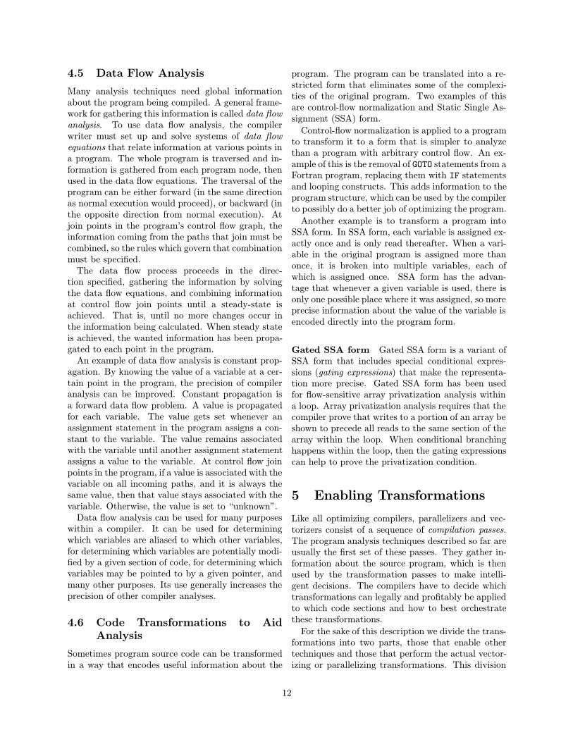
Reduction operations: Reduction operations ab-stract the values of an array into a form with lesserdimensionality. The typical example is an array beingsummed up into a scalar variable. The parallelizingtransformation is shown in Figure 3.

Figure 3: Reduction Parallelization.

The idea for enabling parallel execution of thiscomputation exploits mathematical commutativity.We can split the array into p parts, sum them up in-dividually by different processors, and then combinethe results. The transformed code has two additionalloops, for initializing and combining the partial re-sults. If the size of the main reduction loop (variablen) is large, then these loops are negligible. The mainloop is fully parallel.

More advanced forms of this technique deal witharray reductions, where the sum operation modifiesseveral elements of an array instead of a scalar. Fur-thermore, the summation is not the only possible re-duction operation. Another important reduction isfinding the minimum or maximum value of an array.

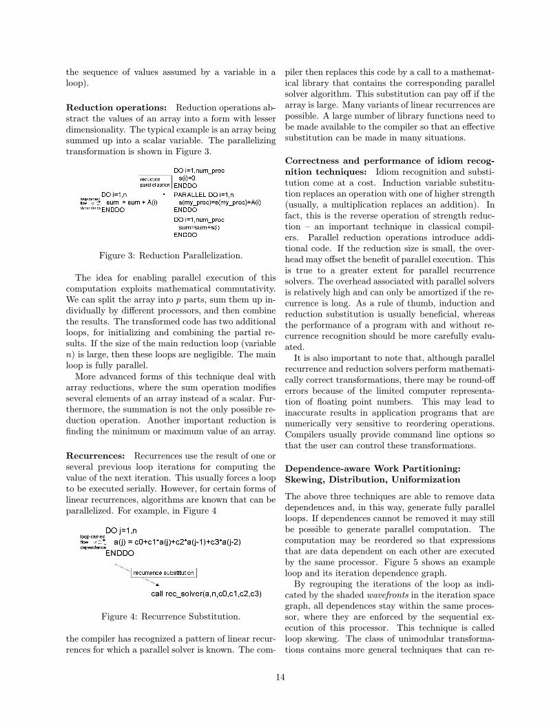
Recurrences: Recurrences use the result of one orseveral previous loop iterations for computing thevalue of the next iteration. This usually forces a loopto be executed serially. However, for certain forms oflinear recurrences, algorithms are known that can beparallelized. For example, in Figure 4

Figure 4: Recurrence Substitution.

the compiler has recognized a pattern of linear recur-rences for which a parallel solver is known. The com-

piler then replaces this code by a call to a mathemat-ical library that contains the corresponding parallelsolver algorithm. This substitution can pay off if thearray is large. Many variants of linear recurrences arepossible. A large number of library functions need tobe made available to the compiler so that an effectivesubstitution can be made in many situations.

Correctness and performance of idiom recog-nition techniques: Idiom recognition and substi-tution come at a cost. Induction variable substitu-tion replaces an operation with one of higher strength(usually, a multiplication replaces an addition). Infact, this is the reverse operation of strength reduc-tion – an important technique in classical compil-ers. Parallel reduction operations introduce addi-tional code. If the reduction size is small, the over-head may offset the benefit of parallel execution. Thisis true to a greater extent for parallel recurrencesolvers. The overhead associated with parallel solversis relatively high and can only be amortized if the re-currence is long. As a rule of thumb, induction andreduction substitution is usually beneficial, whereasthe performance of a program with and without re-currence recognition should be more carefully evalu-ated.

It is also important to note that, although parallelrecurrence and reduction solvers perform mathemati-cally correct transformations, there may be round-offerrors because of the limited computer representa-tion of floating point numbers. This may lead toinaccurate results in application programs that arenumerically very sensitive to reordering operations.Compilers usually provide command line options sothat the user can control these transformations.

Dependence-aware Work Partitioning:Skewing, Distribution, Uniformization

The above three techniques are able to remove datadependences and, in this way, generate fully parallelloops. If dependences cannot be removed it may stillbe possible to generate parallel computation. Thecomputation may be reordered so that expressionsthat are data dependent on each other are executedby the same processor. Figure 5 shows an exampleloop and its iteration dependence graph.

By regrouping the iterations of the loop as indi-cated by the shaded wavefronts in the iteration spacegraph, all dependences stay within the same proces-sor, where they are enforced by the sequential ex-ecution of this processor. This technique is calledloop skewing. The class of unimodular transforma-tions contains more general techniques that can re-

14

Figure 5: Partitioning the Iteration Space in “Wave-front” Manner.

order loop iterations according to various criteria,such as dependence considerations and locality of ref-erence (locality optimizations will be discussed in Sec-tion 7.2).

Other techniques can find partial parallelism inloops that contain data dependences. For example,loop distribution may split a loop into two loops. Oneof them contains all dependent statements and mustexecute serially, while the other one is fully paral-lel. Another example is dependence uniformization,which tries to find minimum dependence distances.If all dependence distances are greater than a thresh-old t, then t consecutive iterations can be executedin parallel.

5.2 Enabling and Enhancing OtherTransformations

Another class of enabling transformations containsprerequisite techniques for other transformations andtechniques that allow others to be applied more ef-fectively. Some transformations belong to both theenabling and enabled techniques. Because of this wewill only give an overview. The following two sectionswill describe details of some of the techniques.

Various transformations require statements to bereordered. This can result in dependence distancesgetting shorter (the producing and consuming state-ments of a value are moved closer together), thepoints of use and reuse of a variable are moved closertogether (which improves cache locality), or back-wards dependences can be turned into forward de-pendences.

Loop distribution splits loops into two or moreloops that can be optimized individually. It alsoenables vectorization, discussed next. Interchang-ing two nested loops can help the vectorization tech-niques, which usually act on the innermost loop.It can also enhance parallelization because moving

a parallel loop to an outer position increases theamount of work inside the parallel region.

Splitting a single loop into a nest of two loops iscalled stripmining or loop blocking. It enables theexploitation of hierarchical parallelism (e.g., the innerloop may then be executed across a multiprocessor,while the outer loop gets executed by a cluster ofsuch multiprocessors.) It is also an important cacheoptimization, as we will discuss.

6 Vectorization: ExploitingVector Architectures

Vectorizing compilers exploit vector architectures bygenerating code that performs operations on a num-ber of data elements in a row. This was of great in-terest in classical supercomputers, which were builtas vector architectures. In addition, vectorization hasenjoyed renewed interest in modern microprocessors,which can accommodate several short data items inone word. For example, a 64 bit word can accommo-date a “vector” of 16 4-bit words. Instructions thatoperate on vectors of this kind are sometimes referredto as multi-media extensions (MMX).

The objective of a vectorizing compiler is to iden-tify and express such vector operations in a form thatcan then be easily mapped onto the vector instruc-tions available in these architectures. A simple ex-ample is shown in Figure 6. The following transfor-mations aid vectorization in more complex programpatterns.

Figure 6: Basic Vectorization.

Scalar Expansion

Private variables, introduced in Section 5.1, need tobe expanded in order to allow vectorization. The fol-lowing shows the privatization example of Section 5.1transformed into vector form.

T(1:n) = A(1:n)+B(1:n)C(1:n) = T(1:n)+T(1:n)**2

15

Loop Distribution

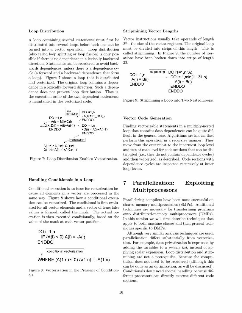
A loop containing several statements must first bedistributed into several loops before each one can beturned into a vector operation. Loop distribution(also called loop splitting or loop fission) is only pos-sible if there is no dependence in a lexically backwarddirection. Statements can be reordered to avoid back-wards dependences, unless there is a dependence cy-cle (a forward and a backward dependence that forma loop). Figure 7 shows a loop that is distributedand vectorized. The original loop contains a depen-dence in a lexically forward direction. Such a depen-dence does not prevent loop distribution. That is,the execution order of the two dependent statementsis maintained in the vectorized code.

Figure 7: Loop Distribution Enables Vectorization.

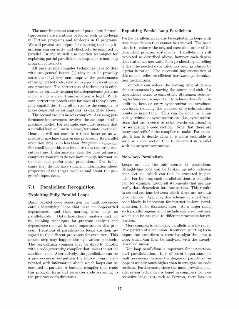
Handling Conditionals in a Loop

Conditional execution is an issue for vectorization be-cause all elements in a vector are processed in thesame way. Figure 8 shows how a conditional execu-tion can be vectorized. The conditional is first evalu-ated for all vector elements and a vector of true/falsevalues is formed, called the mask. The actual op-eration is then executed conditionally, based on thevalue of the mask at each vector position.

Figure 8: Vectorization in the Presence of Condition-als.

Stripmining Vector Lengths

Vector instructions usually take operands of length2n - the size of the vector registers. The original loopmust be divided into strips of this length. This iscalled stripmining. In Figure 9, the number of iter-ations have been broken down into strips of length32.

Figure 9: Stripmining a Loop into Two Nested Loops.

Vector Code Generation

Finding vectorizable statements in a multiply-nestedloop that contains data dependences can be quite dif-ficult in the general case. Algorithms are known thatperform this operation in a recursive manner. Theymove from the outermost to the innermost loop leveland test at each level for code sections that can be dis-tributed (i.e., they do not contain dependence cycles)and then vectorized, as described. Code sections withdependence cycles are inspected recursively at innerloop levels.

7 Parallelization: ExploitingMultiprocessors

Parallelizing compilers have been most successful onshared-memory multiprocessors (SMPs). Additionaltechniques are necessary for transforming programsonto distributed-memory multiprocessors (DMPs).In this section we will first describe techniques thatapply to both machine classes and then present tech-niques specific to DMPs.

Although very similar analysis techniques are used,parallelization differs substantially from vectoriza-tion. For example, data privatization is expressed byadding the variables to a private list, instead of ap-plying scalar expansion. Loop distribution and strip-mining are not a prerequisite, because the compu-tation does not need to be reordered (although thiscan be done as an optimization, as will be discussed).Conditionals don’t need special handling because dif-ferent processors can directly execute different codesections.

16

The most important sources of parallelism for mul-tiprocessors are iterations of loops, such as do-loopsin Fortran programs and for-loops in C programs.We will present techniques for detecting that loop it-erations can correctly and effectively be executed inparallel. Briefly we will also mention techniques forexploiting partial parallelism in loops and in non-loopprogram constructs.

All parallelizing compiler techniques have to dealwith two general issues, (1) they must be provablycorrect and (2) they must improve the performanceof the generated code, relative to a serial execution onone processor. The correctness of techniques is oftenstated by formally defining data-dependence patternsunder which a given transformation is legal. Whilesuch correctness proofs exist for most of today’s com-piler capabilities, they often require the compiler tomake conservative assumptions, as described above.

The second issue is no less complex. Assessing per-formance improvement involves the assumption of amachine model. For example, one must assume thata parallel loop will incur a start/terminate overhead.Hence, it will not execute n times faster on an n-processor machine than on one processor. Its parallelexecution time is no less than

t1 processor

n + toverhead.For small loops this can be more than the serial exe-cution time. Unfortunately, even the most advancedcompilers sometimes do not have enough informationto make such performance predictions. This is be-cause they do not have sufficient information aboutproperties of the target machine and about the pro-gram’s input data.

7.1 Parallelism Recognition

Exploiting Fully Parallel Loops

Basic parallel code generation for multiprocessorsentails identifying loops that have no loop-carrieddependences, and then marking these loops asparallelizable. Data-dependence analysis and allits enabling techniques for program analysis anddependence-removal is most important in this pro-cess. Iterations of parallelizable loops are then as-signed to the different processors for execution. Thissecond step may happen through various methods.The parallelizing compiler may be directly coupledwith a code-generating compiler that issues the actualmachine code. Alternatively, the parallelizer can bea pre-processor, outputting the source program an-notated with information about which loops can beexecuted in parallel. A backend compiler then readsthis program form and generates code according tothe preprocessor’s directives.

Exploiting Partial Loop Parallelism

Partial parallelism can also be exploited in loops withtrue dependences that cannot be removed. The basicidea is to enforce the original execution order of thedependent program statements. Parallelism is stillexploited as described above, however each depen-dent statement now waits for a go-ahead signal tellingit that the needed data value has been produced bya prior iteration. The successful implementation ofthis scheme relies on efficient hardware synchroniza-tion mechanisms.

Compilers can reduce the waiting time of depen-dent statements by moving the source and sink of adependence closer to each other. Statement reorder-ing techniques are important to achieve this effect. Inaddition, because every synchronization introducesoverhead, reducing the number of synchronizationpoints is important. This can be done by elimi-nating redundant synchronizations (i.e., synchroniza-tions that are covered by other synchronizations) orby serializing a code section. Note that there aremany tradeoffs for the compiler to make. For exam-ple, it has to decide when it is more profitable toserialize a code section than to execute it in parallelwith many synchronizations.

Non-loop Parallelism

Loops are not the only source of parallelism.Straight-line code can be broken up into indepen-dent sections, which can then be executed in par-allel. For building such parallel sections, a compilercan, for example, group all statements that are mu-tually data dependent into one section. This resultsin several sections between which there are no datadependences. Applying this scheme at small basiccode blocks is important for instruction-level paral-lelization, to be discussed later. At a larger scale,such parallel regions could include entire subroutines,which can be assigned to different processors for ex-ecution.

More complex is exploiting parallelism in the repet-itive pattern of a recursion. Recursion splitting tech-niques can transform a recursive algorithm into aloop, which can then be analyzed with the alreadydescribed means.

Non-loop parallelism is important for instruction-level parallelization. It is of lesser importance formultiprocessors because the degree of parallelism inloops is usually much higher than in straight-line codesections. Furthermore, since the most prevalent par-allelization technology is found in compilers for non-recursive languages, such as Fortran, there has not

17

been a pressing need to deal with recursive programpatterns.

7.2 Parallel Loop Restructuring

Once parallel loops are detected, there are severalloop transformations that can optimize the programsuch that it (1) exploits the available resources in anoptimal way and (2) minimizes overheads.

Increasing Granularity

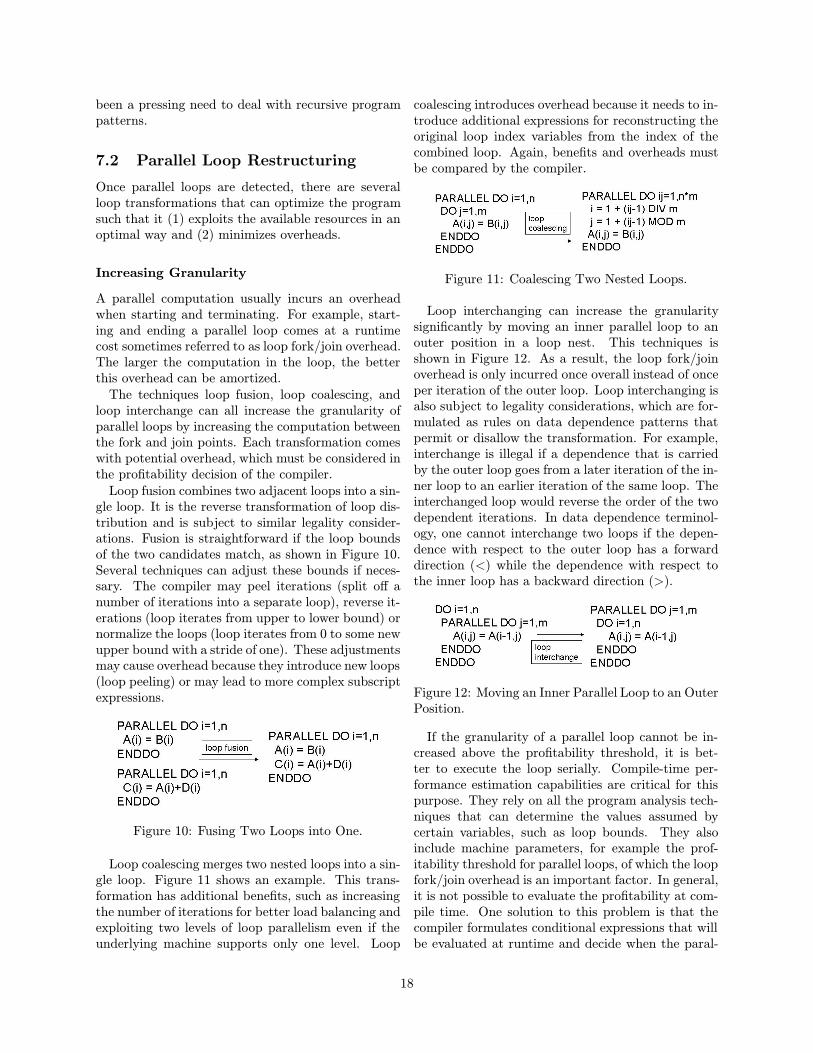
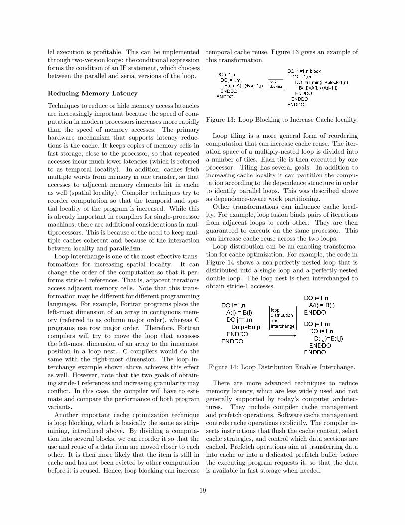
A parallel computation usually incurs an overheadwhen starting and terminating. For example, start-ing and ending a parallel loop comes at a runtimecost sometimes referred to as loop fork/join overhead.The larger the computation in the loop, the betterthis overhead can be amortized.

The techniques loop fusion, loop coalescing, andloop interchange can all increase the granularity ofparallel loops by increasing the computation betweenthe fork and join points. Each transformation comeswith potential overhead, which must be considered inthe profitability decision of the compiler.

Loop fusion combines two adjacent loops into a sin-gle loop. It is the reverse transformation of loop dis-tribution and is subject to similar legality consider-ations. Fusion is straightforward if the loop boundsof the two candidates match, as shown in Figure 10.Several techniques can adjust these bounds if neces-sary. The compiler may peel iterations (split off anumber of iterations into a separate loop), reverse it-erations (loop iterates from upper to lower bound) ornormalize the loops (loop iterates from 0 to some newupper bound with a stride of one). These adjustmentsmay cause overhead because they introduce new loops(loop peeling) or may lead to more complex subscriptexpressions.

Figure 10: Fusing Two Loops into One.

Loop coalescing merges two nested loops into a sin-gle loop. Figure 11 shows an example. This trans-formation has additional benefits, such as increasingthe number of iterations for better load balancing andexploiting two levels of loop parallelism even if theunderlying machine supports only one level. Loop

coalescing introduces overhead because it needs to in-troduce additional expressions for reconstructing theoriginal loop index variables from the index of thecombined loop. Again, benefits and overheads mustbe compared by the compiler.

Figure 11: Coalescing Two Nested Loops.

Loop interchanging can increase the granularitysignificantly by moving an inner parallel loop to anouter position in a loop nest. This techniques isshown in Figure 12. As a result, the loop fork/joinoverhead is only incurred once overall instead of onceper iteration of the outer loop. Loop interchanging isalso subject to legality considerations, which are for-mulated as rules on data dependence patterns thatpermit or disallow the transformation. For example,interchange is illegal if a dependence that is carriedby the outer loop goes from a later iteration of the in-ner loop to an earlier iteration of the same loop. Theinterchanged loop would reverse the order of the twodependent iterations. In data dependence terminol-ogy, one cannot interchange two loops if the depen-dence with respect to the outer loop has a forwarddirection (<) while the dependence with respect tothe inner loop has a backward direction (>).

Figure 12: Moving an Inner Parallel Loop to an OuterPosition.

If the granularity of a parallel loop cannot be in-creased above the profitability threshold, it is bet-ter to execute the loop serially. Compile-time per-formance estimation capabilities are critical for thispurpose. They rely on all the program analysis tech-niques that can determine the values assumed bycertain variables, such as loop bounds. They alsoinclude machine parameters, for example the prof-itability threshold for parallel loops, of which the loopfork/join overhead is an important factor. In general,it is not possible to evaluate the profitability at com-pile time. One solution to this problem is that thecompiler formulates conditional expressions that willbe evaluated at runtime and decide when the paral-

18

lel execution is profitable. This can be implementedthrough two-version loops: the conditional expressionforms the condition of an IF statement, which choosesbetween the parallel and serial versions of the loop.

Reducing Memory Latency

Techniques to reduce or hide memory access latenciesare increasingly important because the speed of com-putation in modern processors increases more rapidlythan the speed of memory accesses. The primaryhardware mechanism that supports latency reduc-tions is the cache. It keeps copies of memory cells infast storage, close to the processor, so that repeatedaccesses incur much lower latencies (which is referredto as temporal locality). In addition, caches fetchmultiple words from memory in one transfer, so thataccesses to adjacent memory elements hit in cacheas well (spatial locality). Compiler techniques try toreorder computation so that the temporal and spa-tial locality of the program is increased. While thisis already important in compilers for single-processormachines, there are additional considerations in mul-tiprocessors. This is because of the need to keep mul-tiple caches coherent and because of the interactionbetween locality and parallelism.

Loop interchange is one of the most effective trans-formations for increasing spatial locality. It canchange the order of the computation so that it per-forms stride-1 references. That is, adjacent iterationsaccess adjacent memory cells. Note that this trans-formation may be different for different programminglanguages. For example, Fortran programs place theleft-most dimension of an array in contiguous mem-ory (referred to as column major order), whereas Cprograms use row major order. Therefore, Fortrancompilers will try to move the loop that accessesthe left-most dimension of an array to the innermostposition in a loop nest. C compilers would do thesame with the right-most dimension. The loop in-terchange example shown above achieves this effectas well. However, note that the two goals of obtain-ing stride-1 references and increasing granularity mayconflict. In this case, the compiler will have to esti-mate and compare the performance of both programvariants.

Another important cache optimization techniqueis loop blocking, which is basically the same as strip-mining, introduced above. By dividing a computa-tion into several blocks, we can reorder it so that theuse and reuse of a data item are moved closer to eachother. It is then more likely that the item is still incache and has not been evicted by other computationbefore it is reused. Hence, loop blocking can increase

temporal cache reuse. Figure 13 gives an example ofthis transformation.

Figure 13: Loop Blocking to Increase Cache locality.

Loop tiling is a more general form of reorderingcomputation that can increase cache reuse. The iter-ation space of a multiply-nested loop is divided intoa number of tiles. Each tile is then executed by oneprocessor. Tiling has several goals. In addition toincreasing cache locality it can partition the compu-tation according to the dependence structure in orderto identify parallel loops. This was described aboveas dependence-aware work partitioning.

Other transformations can influence cache local-ity. For example, loop fusion binds pairs of iterationsfrom adjacent loops to each other. They are thenguaranteed to execute on the same processor. Thiscan increase cache reuse across the two loops.

Loop distribution can be an enabling transforma-tion for cache optimization. For example, the code inFigure 14 shows a non-perfectly-nested loop that isdistributed into a single loop and a perfectly-nesteddouble loop. The loop nest is then interchanged toobtain stride-1 accesses.

Figure 14: Loop Distribution Enables Interchange.

There are more advanced techniques to reducememory latency, which are less widely used and notgenerally supported by today’s computer architec-tures. They include compiler cache managementand prefetch operations. Software cache managementcontrols cache operations explicitly. The compiler in-serts instructions that flush the cache content, selectcache strategies, and control which data sections arecached. Prefetch operations aim at transferring datainto cache or into a dedicated prefetch buffer beforethe executing program requests it, so that the datais available in fast storage when needed.

19

Multi-level Parallelization

Most multiprocessors today offer one-level paral-lelism. That means that, usually, a single loop out ofa loop nest can be executed in parallel. Architecturesthat have a hierarchical structure can exploit two ormore levels of parallelism. For example, a cluster ofmultiprocessors may be able to execute two nestedparallel loops, the outer one across the clusters whilethe inner loop employs the processors within eachcluster.

Program sections that contain singly-nested loopscan be turned into two-level parallelism by stripmin-ing them into two nested loops as shown in Figure 15.

Figure 15: Stripmining Enables 2-level Parallelism.

7.3 Scheduling

After parallelism is detected and loops are restruc-tured for optimal performance, there is still the issueof defining an execution order and assigning parallelactivities to processors. This must be done in a waythat (1) balances the load, (2) performs computationwhere the necessary resources are, and (3) considersthe environment. Scheduling decisions can be done atcompile time (statically) or at runtime (dynamically).Both methods have advantages and disadvantages.

Load balancing is the primary reason for dynamicscheduling. Static scheduling methods typically splitup the number of loop iterations into equal chunksand assign them to the different processors. Thisworks well if the loop iterations are equal in size.However this is not the case in loops that containconditional statements or in an inner loop of a nestwhose number of iterations depends on an outer loopvariable. Dynamic scheduling methods assign loop it-erations to processors, a chunk at a time. The chunkcan contain one or more iterations. Of special inter-est are also scheduling schemes that vary the chunksize, such as trapezoidal scheduling and guided selfscheduling methods. Dynamic scheduling methodscome with some runtime overhead for performing the

scheduling action. However this is often negligiblecompared to the gain from load balancing.

The goal of computing where the resources are, onthe other hand, favors static scheduling methods. Inheterogeneous systems it is mandatory to perform thecomputation where necessary processor capabilitiesor input/output devices are. In multiprocessors, dataare critical resources, whose location may determinethe best executing processor. For example, if a dataitem is known to be in the cache of a specific pro-cessor, then it is best to execute other computationsaccessing the same data item on the same processoras well. The compiler has knowledge of which com-putation accesses which data in the future. Hence,such scheduling decisions are good to make at com-pile time. In distributed-memory systems this situa-tion is even more pronounced. Accessing a data itemon a processor other than its owner, involves commu-nication with high latencies.

Scheduling decisions also depend on the environ-ment of the machine. For example, in a single-userenvironment it may be best to statically schedulecomputation that is known to execute evenly. How-ever if the same program is executed in a multi-userenvironment, the load of the processors can be veryuneven, making dynamic scheduling methods the bet-ter option.

7.4 Techniques Specific to DMPs

Distributed-memory multiprocessors do not providea shared address space. Many of the techniques de-scribed so far assume that all computation can see thenecessary data, no matter where it is performed. InDMPs this is no longer the case. The compiler needsto distribute the program’s data onto several computenodes, and data items that are needed by nodes otherthan their home need to be communicated by send-ing and receiving messages. This creates two majornew tasks for the compiler: (1) finding a good datapartitioning and distribution scheme, and (2) orches-trating the communication between the nodes in anoptimal way.

Data Partitioning and Distribution

The goal of data partitioning and distribution is toplace each data item on the compute node that ac-cesses it most frequently. Data partitioning and dis-tribution are often performed as two or more stepsin a compiler. For simplicity we describe it here asone data distribution step. Several issues need to beresolved. First, the proper units of data distributionneed to be determined. Typically these are sections

20

of arrays. Second, data access costs and frequenciesneed to be estimated to compare distribution alter-natives. Third, if there are program sections withdifferent access patterns, redistribution may need tobe considered at runtime.

The simplest data distribution scheme is block dis-tribution, which divides an array into p sections,where p is the number of processors. Block distribu-tion creates contiguous array sections on each proces-sor. If adjacent processors access adjacent array ele-ments, then cyclic distribution is appropriate. Block-cyclic distribution is a combination of both schemes.For irregular access patterns, indexed distributionmay be most appropriate. Figure 16 illustrates thesedistribution schemes.

Figure 16: Data Distribution Schemes.Numbers indi-cate the node of a 4-processor DMP on which the array sectionis placed.

A major difficulty is that data distribution deci-sions affect all program sections accessing a givendata element. Hence, global optimizations need tobe performed, which can be algorithmically complex.Furthermore, compile-time information about arrayaccesses is often incomplete. Better global optimiza-tion would require knowledge of the program inputdata. Also, distribution decisions cannot be made inisolation. They need to factor in available parallelismand the cost of messages, described next. Finally,indexed distribution, although most flexible, may in-cur additional overhead because the index array mayneed to be distributed itself, causing double latenciesfor each array access. Because of all this, develop-ing compiler techniques for automatic data partition-ing and distribution is still an active research topic.Many current parallel programming approaches as-sume that the user assists the compiler in this pro-cess.

Message Generation

Once the owner processor for each data item is identi-fied, the compiler needs to determine which accessesare from remote processors and then insert communi-cation to and from these processors. The most com-

mon form of communication is to send and receivemessages, which can communicate one or several dataelements between two specific processors. More com-plex communication primitives are also known, suchas broadcasts (send to all processors) and reductions(receive from all processors and combine the resultsin some form).

The basic idea of message generation is simple.Each statement needs to communicate to/from re-mote processors the accessed data elements that arenot local. Often, the owner-computes principle is as-sumed. For example, assignment statements are ex-ecuted on the processor that owns the left-hand-sideelement. (Note that this execution scheme is differ-ent from the one assumed for SMPs, where an entireloop iteration is executed by one and the same pro-cessor.) Data partitioning information hence suppliesboth the information about which processor executeswhich statement and what data is local/remote. TheFigure 17 shows the basic messages generated. It as-sumes a block partitioning of both arrays, A and B.

Figure 17: Generating Messages for Data Exchangein a Distributed-Memory Machine.

Although generating messages in this schemewould lead to a functionally correct program, thisprogram may be inefficient. To increase the effi-ciency, the compiler needs to aggregate communi-cation. That is, messages generated for individualstatements need to be combined into a larger mes-sage. Also, messages may be moved to an earlierpoint in the instruction stream, so that communi-cation latencies can be overlapped with computa-tion. Message aggregation for the general block-cyclicdistribution is already rather complex. It is madeeven more difficult because message sizes may onlybe known in the form of symbolic expressions. Forindexed distributions, support through “communica-tion libraries for irregular computation” has been anactive research topic. In general, compilers that dealwith the issues of message generation for DMPs arehighly sophisticated and complex.

21

8 Exploiting Parallelism at theInstruction Level

Instruction-level parallelism (ILP) refers to the pro-cessor’s capability to execute several instructions atthe same time. Instruction-level parallelism can beexploited implicitly by the processor without thecompiler issuing special directives or instructions tothe hardware. Or, the compiler can extract par-allelism explicitly and express it in the generatedcode. Examples of the latter type of generated codeare Very-Long Instruction Word (VLIW) or Explic-itly Parallel Instruction Computing (EPIC) architec-tures. In addition to the techniques presented here,all or most techniques known from classical compilersare important and are often applied as a first set oftransformations and analysis passes in ILP compilers(see “Program Compilers”).

8.1 Implicit Instruction-level Paral-lelism

For implicit instruction-level parallelism,the compiler-generated code can be the same as forsingle-issue machines. However, knowing the proces-sor’s ILP mechanisms, the compiler can change thecode so that the processor can do a more effectivejob. Three categories of techniques are importantfor this objective, (1) scheduling instructions, (2) re-moving dependences, and (3) increasing the windowsize within which the processor can exploit parallelinstructions.

Instruction Scheduling

Modern processors exploit ILP by starting a new in-struction before an earlier instruction has completed.All instructions begin their execution in the orderdefined by the program. This order can have a sig-nificant performance impact. Hence, an importanttask of the compiler is to define a good order. It doesthis by moving instructions that incur long latenciesprior to those with short latencies. Such instructionscheduling is subject to data dependence constraints.For example, an instruction consuming a value in aregister or memory must not be moved before an in-struction producing this value. Instruction schedul-ing is a well-established technology, discussed in stan-dard compiler textbooks. We refer the reader to suchliterature for further details.

Removing Dependences

The basic patterns for removing dependences are sim-ilar to the ones discussed for loop-level parallelism.Anti dependences can be removed through variablerenaming techniques. In addition, register renamingbecomes important. It avoids conflicts between po-tentially parallel sets of instructions that make useof the same register for storing temporary values.Such techniques can be opposite from good registerallocation in sequential instruction streams, wherenon-overlapping life times of different variables areassigned to the same register. Because of this, thecompiler may rely on hardware register-renaming ca-pabilities available in the processor.

Similar to the induction variable recognition tech-nique discussed above, the compiler can replace in-cremental operations through operations that useoperands available at the beginning of a parallel codesection. Likewise, a sequence of sum operations maybe replaced by sum operations into a temporary vari-able, followed by an update step at the end of theparallel region. Figure 18 illustrates these transfor-mations.

Figure 18: Dependence-Removing Transformationfor Instruction-Level Parallelism.Shaded blocks of in-structions are independent of each other and can be executedin parallel.

Increasing the Window Size

A large window of instructions within which the pro-cessor can discover and exploit ILP is important fortwo reasons. First, it leads to more opportunities forparallelism and, second, it reduces the relative cost ofstarting the instruction pipeline, which usually hap-pens at window boundaries.

Window boundaries are typically branch instruc-tions. Instruction analysis and parallel execution can-

22

not easily cross branch instructions because the pro-cessor does not know what instructions will executeafter the branch until it is reached. For example,an instruction may only execute on the true branchof a conditional jump. Hence, although the instruc-tion could be executed in parallel with another in-struction before the branch, this is not feasible. Ifthe false branch is taken, the instruction might havewritten an undesired value to memory. Even if allside effects of such instructions were kept in tempo-rary storage, they may raise exceptions that couldincorrectly abort program execution.

There are several techniques for increasing the win-dow size. Code motion techniques can move instruc-tions across branches under certain conditions. Forexample, if the same instruction appears on bothbranches it can be moved before the branch, subjectto data dependence considerations. In this way, thebasic block on the critical path can be increased oranother basic block can be completely removed.

Instruction predication can also remove a branch byassigning the branch condition to a mask, which thenguards the merged statements of both branches. Fig-ure 19 shows an example. Predicated execution needshardware support and the compiler must tradeoff thebenefits of enhanced ILP with the overhead of moreexecuted instructions.

Figure 19: Generating Predicated Code.

Basically, ILP is exploited in straight-line codesections. Additional performance can be gainedwhen exploiting parallelism across loop iterations. Astraightforward way to achieve this is to unroll loopiterations, that is, to replicate the loop body by afactor n (and divide the number of iterations by thesame factor). Many techniques that were discussedunder loop optimizations for multiprocessors are ap-plicable to this case as well.

8.2 Explicit Instruction-level Paral-lelism

The basic techniques for removing dependences andincreasing the window size are important for explicitILP as well. However the goal is no longer to exposemore parallelism to the hardware detection mecha-nisms, but to make parallelism more analyzable bythe compiler itself. As an example of explicit ILP we

choose a VLIW architecture and a software pipeliningtechnique. The goal is to find a repetitive instructionpattern in a loop that can be mapped efficiently to asequence of VLIW instructions. It is called pipelin-ing because the execution may “borrow” instructionsfrom earlier or later iterations to fill an efficient sched-ule. Hence the execution of parts of different itera-tions overlap with each other. This is illustrated inFigure 20. The reader may notice that there would bea conflict in register use between the overlapping loopiterations. For example, in the same VLIW instruc-tion s4 uses R0’s value of one loop iteration while s2uses R0’s value belonging to the next iteration. Bothsoftware and hardware register renaming techniquesare known to resolve this problem.

Figure 20: Translating a Loop in a Software PipelingScheme.

Efficient parallelism at the instruction level de-pends on the compiler’s ability to identify code se-quences that are executed with high probability. Theinstructions of these code sequences must then bereordered so that the processor’s functional unitsare exploited in an optimal way. The two tasksare sometimes called trace selection and trace com-paction, respectively. Trace selection is a global op-timization in that it looks for code sequences acrossmultiple branches, factoring in estimated branch fre-quences. Trace compaction can move instructionsacross branches, whereby it may add bookkeepingcode to ensure correct execution if a predicted branchis not taken. The two techniques together are referredto as trace scheduling.

9 Compiler-internal Concerns

Compiler developers have to resolve a number ofissues other than designing analysis and transfor-

23

mation techniques. These issues become importantwhen creating a complete compiler implementation,in which the described techniques are integrated intoa user-friendly tool. Several compiler research in-frastructures have played pioneering roles in this re-gard. Among them are the Parafrase [1, 2], PFC [3],PTRAN [4], ParaScope [5], Polaris [6], and SUIF [7]compilers. The following paragraphs describe a num-ber of issues that have to be addressed by such in-frastructures. An adequate compiler-internal repre-sentation of the program must be chosen, the largenumber of transformation passes need to be put in theproper order, and decisions have to be made aboutwhere to apply which transformation, so as to max-imize the benefits but keep the compile time withinbounds. The user interface of the compiler is im-portant as well. Optimizing compilers typically comewith a large set of command-line flags, which shouldbe presented in a form that makes them as easy touse as possible.

Internal Representation

A large variety of compiler-internal program repre-sentations (IRs) are in use. They differ with re-spect to the level of program translation and thetype of program analysis information that is implic-itly represented. Several IRs may be used for severalphases of the compilation. The syntax tree IR rep-resents the program at a level that is close to theoriginal program. At the other end of the spectrumare representations close to the generated machinecode. An example of an IR in between these extremesis the register transfer language, which is used bythe widely-available GNU C compiler. Source-leveltransformations, such as loop analysis and transfor-mations, are usually applied on an IR at the levelof the syntax-tree, whereas instruction-level transfor-mations are applied on an IR that is closer to thegenerated machine code. Examples of representationsthat include analysis information are the static singleassignment form (SSA) and the program dependencegraph (PDG). SSA was introduced in Section 4. ThePDG includes information about both data depen-dences and control dependences in a common rep-resentation. It facilitates transformations that needto deal with both types of dependences at the sametime.

Phase Ordering

Many compiler techniques are applied in an obviousorder. Data dependence analysis needs to come be-fore parallel loop recognition, and so do dependence

removing transformations. Other techniques mutu-ally influence each other. We have introduced sev-eral techniques where this situation occurs. For ex-ample, loop blocking for cache locality also involvedloop interchanging, and loop interchanging was madepossible through loop distribution. There are manysituations where the order of transformations is noteasy to determine. One possible solution is for thecompiler to generate internally a large number of pro-gram variants and then estimate their performance.We have already described the difficulty of perfor-mance estimation. In addition, generating a largenumber of program variants may get prohibitively ex-pensive in terms of both compiler execution time andspace need. Practical solutions to the phase orderingproblem are based on heuristics and ad-hoc strate-gies. Finding better solutions is still a research issue.One approach is for the compiler to decide on theapplicability of several transformations at once. Thisis the goal of unimodular transformations, which candetermine a best combination of iteration-reorderingtechniques, subject to data dependence constraints.

Applying Transformations at the Right Place

One of the most difficult problems for compilers isto decide when and where to apply a specific tech-nique. In addition to the phase ordering problem,there is the issue that most transformations can havea negative performance impact if applied to the wrongprogram section. For example, a very small loop mayrun slower in parallel than serially. Interchanging twoloops may increase the parallel granularity but reducedata locality. Stripmining for multi-level parallelismmay introduce more overhead than benefit if the loophas a small number of iterations. This difficulty isincreased by the fact that machine architectures aregetting more complex, requiring specialized compilertransformations in many situations. Furthermore, anincreasing number of compiler techniques are beingdeveloped that apply to a specific program pattern,but not in general. For reasons discussed before, thecompiler does not always have sufficient informationabout the program input data and machine parame-ters to make optimal decisions.

Speed versus Degree of Optimization

Ordinary compilers transform medium-size programsin a few seconds. This is not so for parallelizing com-pilers. Advanced program analysis methods, such asdata dependence analysis and symbolic range anal-ysis, may take significantly longer. In addition, asmentioned above, compilers may need to create sev-

24

eral optimization variants of a program and then pickthe one with the best estimated performance. Thiscan further multiply the compilation time. It raises anew issue in that the compiler now needs to make de-cisions about which program sections to optimize tothe fullest of its capabilities and where to save compi-lation time. One way of resolving this issue is to passthe decision on to the user, in the form of commandline flags.

Compiler Command Line Flags

Ideally, from the user’s point of view – and as anultimate research goal – a compiler would not needany command line flags. It would make all decisionsabout where to apply which optimization techniquefully automatically. Today’s compilers are far fromthis goal. Compiler flags can be seen as one way forthe compiler to gather additional knowledge that isunavailable in the program source code. They maysupply information that otherwise would come fromprogram input data (e.g., the most frequently exe-cuted program sections), from the machine environ-ment (e.g., the cache size), or from application needs(e.g., degree of permitted roundoff error). They mayalso express user preferences (e.g., compilation speedversus degree of optimization). A parallelizing com-piler can include several tens of command line op-tions. Reducing this number can be seen as an im-portant goal for the future generation of vectorizingand parallelizing compilers.

References

[1] D. J. Kuck, R. H. Kuhn, B. Leasure, and M.Wolfe, “The structure of an advanced vectorizerfor pipelined processors,” Proc. of COMPSAC 80,The 4th Int’l. Computer Software and Applica-tions Conference, 1980, pages 709–715.

[2] C. Poly-chronopoulos, M. Girkar, M. R. Haghighat, C.-L.Lee, B. Leung, and D. Schouten, “Parafrase-2: anew generation parallelizing compiler,” Proc. ofthe 1989 Int’l. Conference on Parallel Processing,St. Charles, Ill., 1998, Volume II, pages 39–48.

[3] J.R. Allen and K. Kennedy, “PFC: a program toconvert Fortran to parallel form,” In K. Hwang(ed.), Supercomputers: Design and Applications,IEEE Computer Society Press, 1985, pages 186–205.

[4] F. Allen, M. Burke, P. Charles, R. Cytron, andJ. Ferrante”, “An overview of the PTRAN analy-sis system for multiprocessing,” Proc. of the Int’lConf. on Supercomputing, 1987, pages 194–211.

[5] V. Balasundaram, K. Kennedy, U. Kremer, K.McKinley, and J. Subhlok, “The ParaScope ed-itor: an interactive parallel programming tool,”Proc. of the Int’l Conf. on Supercomputing, 1989,pages 540–550.

[6] W. Blume, R. Doallo, R. Eigenmann, J. Grout,J. Hoeflinger, T. Lawrence, J. Lee, D. Padua, Y.Paek, B. Pottenger, L. Rauchwerger, and PengTu, “Parallel Programming with Polaris.” IEEEComputer, Volume 29, Number 12, pages 78–82,December 1996.

[7] M. W. Hall, J. M. Anderson, S. P. Amarasinghe,B. R. Murphy, S.-W. Liao, E. Bugnion, and M.S. Lam, “Maximizing multiprocessor performancewith the SUIF compiler,” IEEE Computer, Vol-ume 29, Number 12, pages 84–89, December 1996.

Further Reading

• U. Banerjee, R. Eigenmann, A. Nicolau, andD. Padua, “Automatic Program Paralleliza-tion.” Proceedings of the IEEE, 81(2) pages211–243, February 1993.

• B. R. Rau and J. A. Fisher, “Instruction-Level Parallel Processing: History,Overview, and Perspective,” The Journal ofSupercomputing, 7, 9–50, 1993.

• G. Almasi and A. Gottlieb, “Highly Paral-lel Computing,” The Benjamin/CummingsPublishing Company, Inc., 1994.

• U. Banerjee, “Dependence Analysis,”Kluwer Academic Publishers, Boston Mass.,1997.

• J. Hennessy and D. Patterson, “ComputerArchitecture: A Quantitative Approach,”Morgan Kaufmann Publishers, 1996.

• K. Kennedy, “Advanced Compiling for HighPerformance,” Morgan Kaufmann Publish-ers, 2001.

• D. J. Kuck, “High Performance Computing,Challenges for Future Systems,” Oxford Uni-versity Press, New York, 1996.

• M. Wolfe, “High-Performance Compilers forParallel Computing,” Addison-Wesley, 1996.

25

• H. Zima, “Supercompilers for Parallel andVector Computers,” Addison-Wesley, 1991.

26