Page 1
Parallel Time-Domain Boundary Element Methodfor 3-Dimensional Wave Equation
PinT 2015, Dresden, May 28, 2015
D. Lukas, M. Merta, J. Zapletal, and A. Veit
VSB–Technical University of Ostrava, Czech Rep.University of Chicago
email: [email protected]
Page 2
Parallel Time-Domain Boundary Element Methodfor 3-Dimensional Wave Equation
Outline
• Parallel fast BEM and applications
• Boundary integral formulation of sound-hard scattering
• Time-domain boundary element method
• Parallelization, preconditioning, numerical experiments
• Conclusion, outlook, references
Page 3
Parallel Time-Domain Boundary Element Methodfor 3-Dimensional Wave Equation
Outline
• Parallel fast BEM and applications
• Boundary integral formulation of sound-hard scattering
• Time-domain boundary element method
• Parallelization, preconditioning, numerical experiments
• Conclusion, outlook, references
Page 4
Parallel fast BEM and applications
Laplace equation with mixed boundary conditions
Ω ⊂ R2 lipschitz domain, Γ := ∂Ω = ΓD ∪ ΓN, ΓD ∩ ΓN = ∅
−u(x) = 0, x ∈ ΩγD u(x) := u(x) = g(x), x ∈ ΓD
γN u(x) :=dudn(x) = h(x), x ∈ ΓN
Fundamental solution
G(x,y) := −1
2πln ‖x− y‖ satisfies −yG(x,y) = δx in the distributional sense
Representation formula (”v(y) := G(x,y)”)
∀x ∈ Ω : u(x) =
∫
Γ
γNu(y)G(x,y) dl(y)−
∫
Γ
u(y) γN,yG(x,y) dl(y)
We are left to calculate u on ΓN and γNu on ΓD.
Page 5
Parallel fast BEM and applications
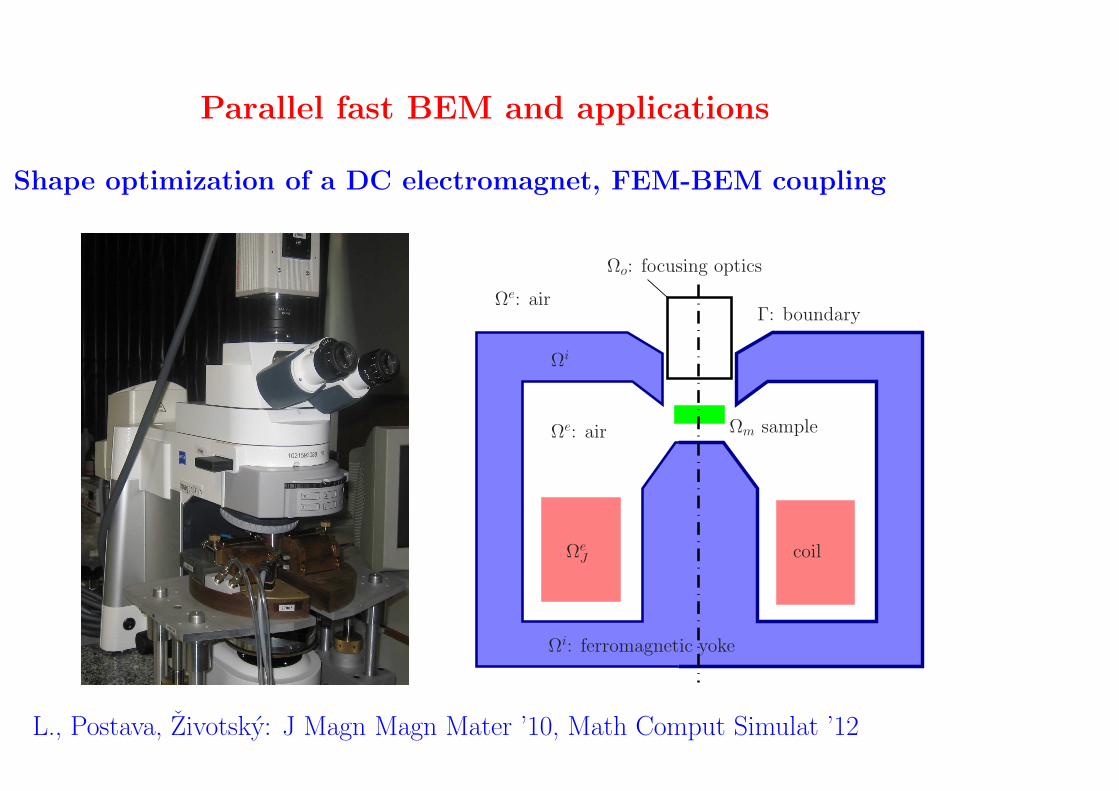
Shape optimization of a DC electromagnet, FEM-BEM coupling
Ωi: ferromagnetic yoke
Ωi
Ωe: air
Ωe: air
Ωe
Jcoil
Ωm sample
Ωo: focusing optics
Γ: boundary
L., Postava, Zivotsky: J Magn Magn Mater ’10, Math Comput Simulat ’12
Page 6
Parallel fast BEM and applications
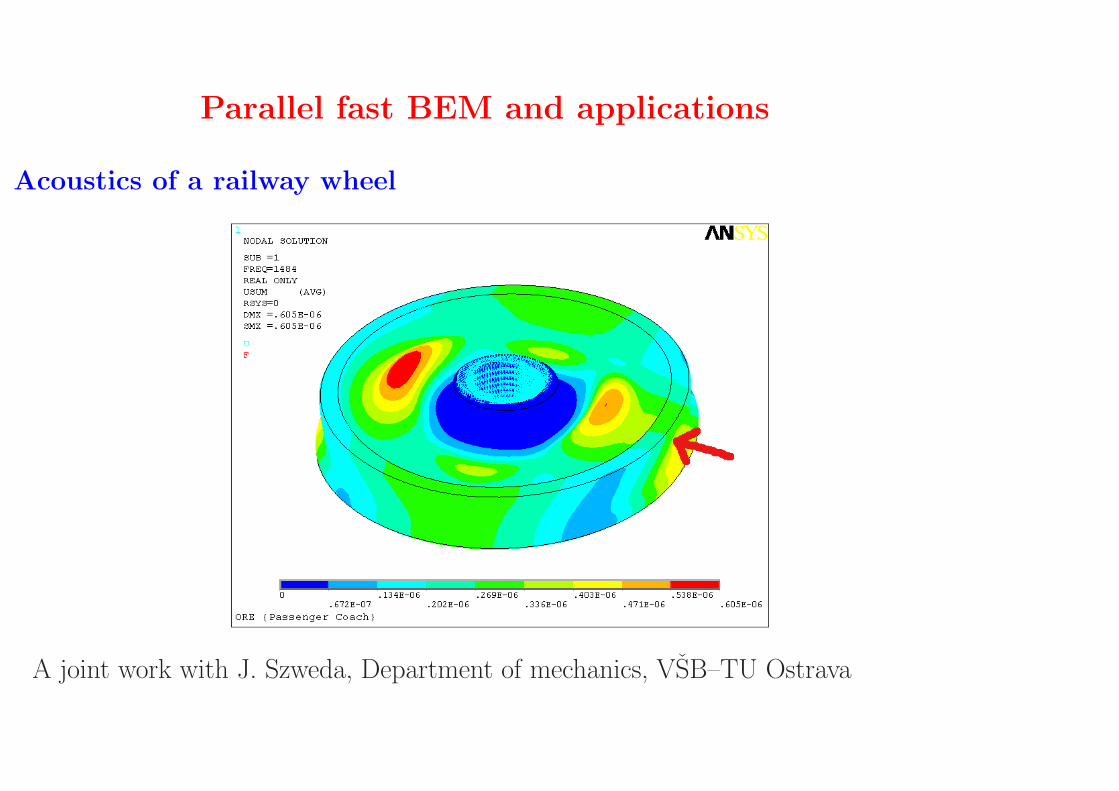
Acoustics of a railway wheel
A joint work with J. Szweda, Department of mechanics, VSB–TU Ostrava
Page 7
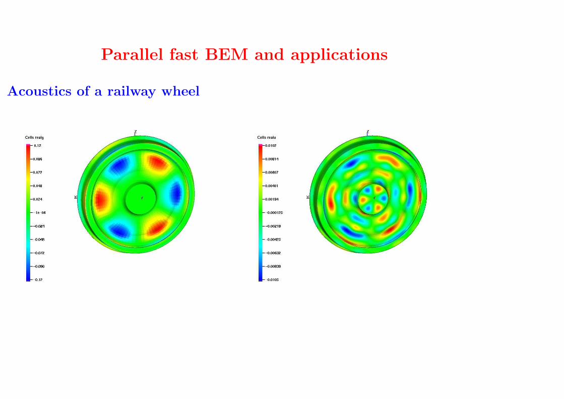
Parallel fast BEM and applications
Acoustics of a railway wheel
Page 8
Parallel fast BEM and applications
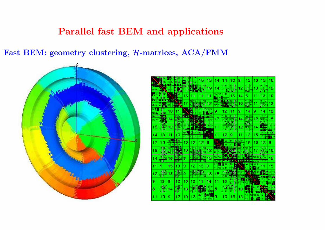
Fast BEM: geometry clustering, H-matrices, ACA/FMM
Page 9
Parallel fast BEM and applications
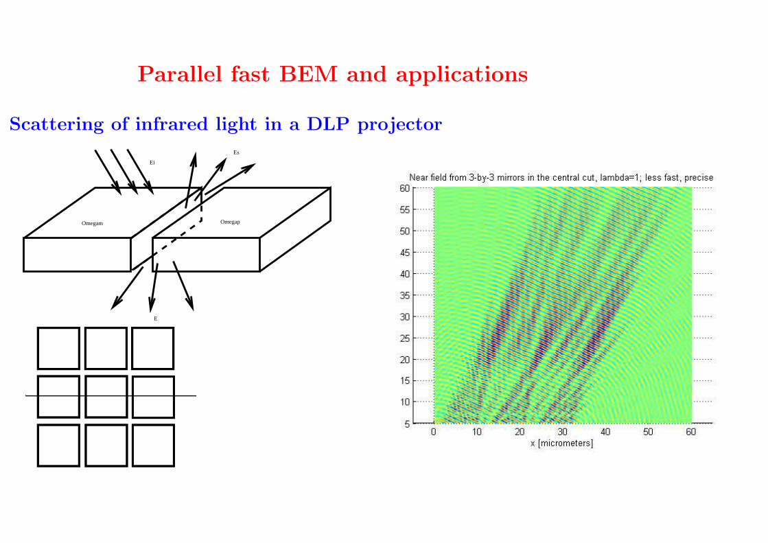
Scattering of infrared light in a DLP projector
Ei
Es
Omegam Omegap
E
Page 10
Parallel fast BEM and applications
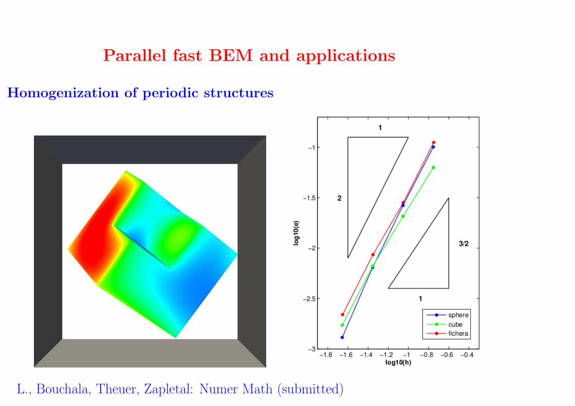
Homogenization of periodic structures
L., Bouchala, Theuer, Zapletal: Numer Math (submitted)
Page 11
Parallel fast BEM and applications
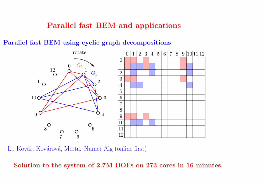
Parallel fast BEM using cyclic graph decompositions
01
2
3
4
5
67
8
9
10
11
12
rotate
G0
G1
0
0
1
1
2
2
3
3
4
4
5
5
6
6
7
7
8
8
9
9
10
10
11
11
12
12
L., Kovar, Kovarova, Merta: Numer Alg (online first)
Solution to the system of 2.7M DOFs on 273 cores in 16 minutes.
Page 12
Parallel fast BEM and applications
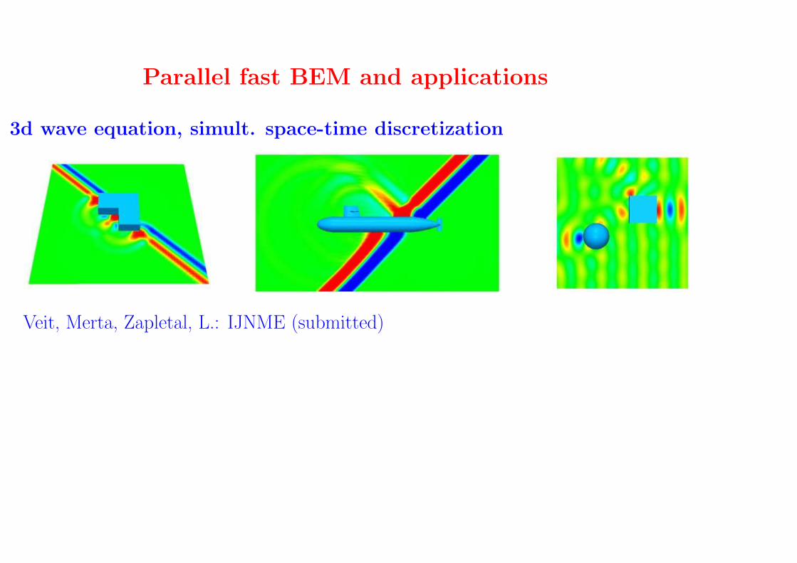
3d wave equation, simult. space-time discretization
Veit, Merta, Zapletal, L.: IJNME (submitted)
Page 13
Parallel Time-Domain Boundary Element Methodfor 3-Dimensional Wave Equation
Outline
• Parallel fast BEM and applications
• Boundary integral formulation of sound-hard scattering
• Time-domain boundary element method
• Parallelization, preconditioning, numerical experiments
• Conclusion, outlook, references
Page 14
Boundary integral formulation of sound-hard scattering
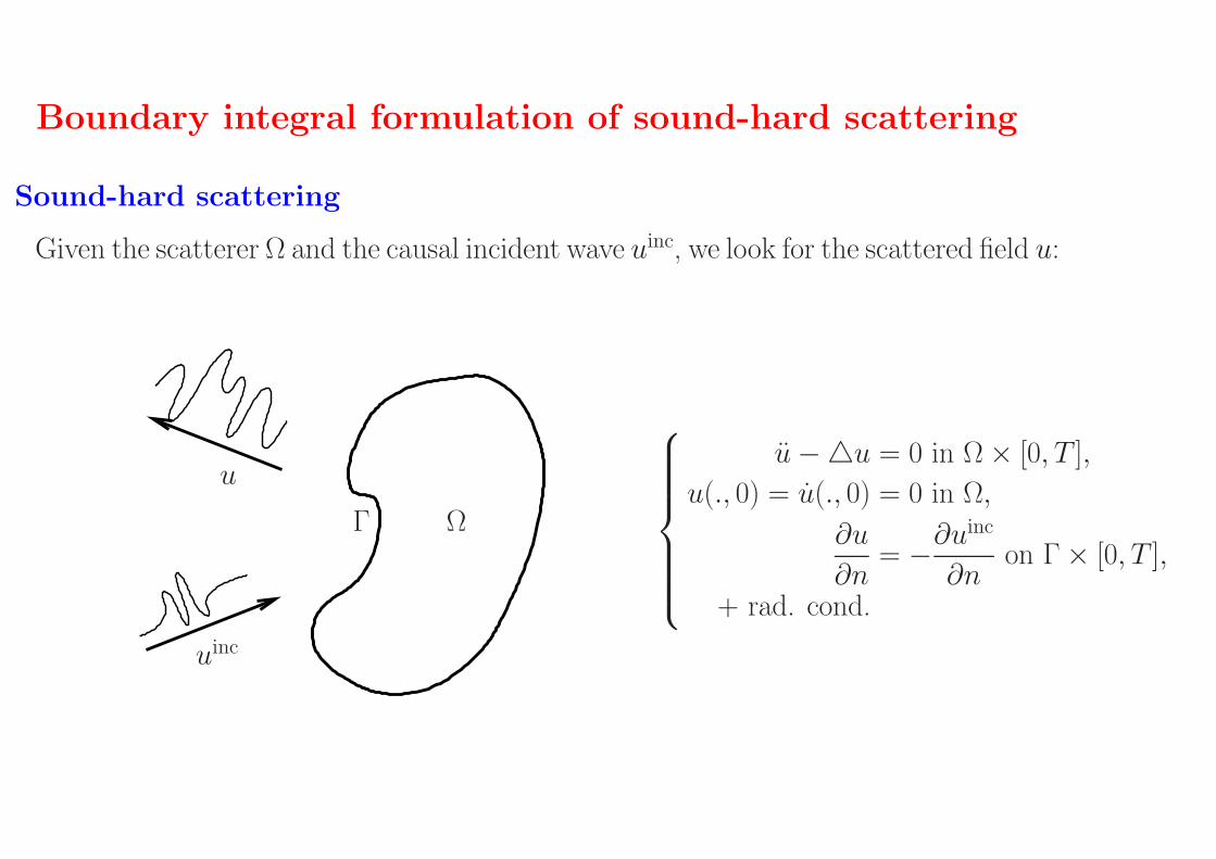
Sound-hard scattering
Given the scatterer Ω and the causal incident wave uinc, we look for the scattered field u:
uinc
u
Γ Ω
u−u = 0 in Ω× [0, T ],
u(., 0) = u(., 0) = 0 in Ω,
∂u
∂n= −
∂uinc
∂non Γ× [0, T ],
+ rad. cond.
Page 15
Boundary integral formulation of sound-hard scattering
Boundary integral ansatz
We search for u in the form of the retarded double-layer potential
u(x, t) = −1
4π
∫
Γ
n(y) · (x− y)
‖x− y‖
(φ(y, t− ‖x− y‖)
‖x− y‖2+φ(y, t− ‖x− y‖)
‖x− y‖
)dS(y),
which satisfies the wave equation and the initial conditions. It remains to fulfill theNeumann boundary condition
limΩ∋x→x∈Γ
n(x) · ∇xu(x, t)︸ ︷︷ ︸
=:(Wφ)(x,t)
= g(x, t) on Γ× [0, T ],
where g := −∂uinc
∂n.
Page 16
Boundary integral formulation of sound-hard scattering
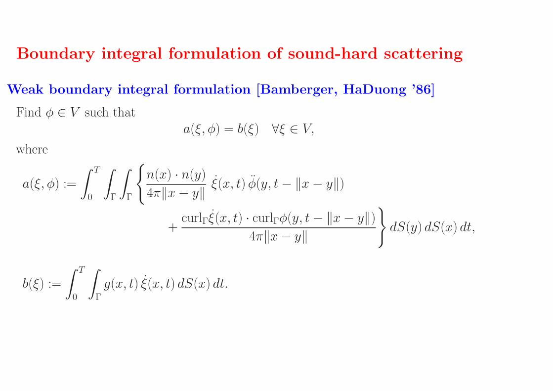
Weak boundary integral formulation [Bamberger, HaDuong ’86]
Find φ ∈ V such thata(ξ, φ) = b(ξ) ∀ξ ∈ V,
where
a(ξ, φ) :=
∫ T
0
∫
Γ
∫
Γ
n(x) · n(y)
4π‖x− y‖ξ(x, t) φ(y, t− ‖x− y‖)
+curlΓξ(x, t) · curlΓφ(y, t− ‖x− y‖)
4π‖x− y‖
dS(y) dS(x) dt,
b(ξ) :=
∫ T
0
∫
Γ
g(x, t) ξ(x, t) dS(x) dt.
Page 17
Parallel Time-Domain Boundary Element Methodfor 3-Dimensional Wave Equation
Outline
• Parallel fast BEM and applications
• Boundary integral formulation of sound-hard scattering
• Time-domain boundary element method
• Parallelization, preconditioning, numerical experiments
• Conclusion, outlook, references
Page 18
Time-domain boundary element method
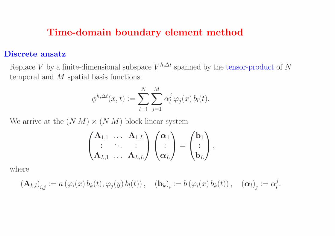
Discrete ansatz
Replace V by a finite-dimensional subspace V h,∆t spanned by the tensor-product of Ntemporal and M spatial basis functions:
φh,∆t(x, t) :=N∑
l=1
M∑
j=1
αjl ϕj(x) bl(t).
We arrive at the (N M)× (N M) block linear systemA1,1 . . . A1,L... . . . ...
AL,1 . . . AL,L
α1...αL
=
b1...bL
,
where
(Ak,l)i,j := a (ϕi(x) bk(t), ϕj(y) bl(t)) , (bk)i := b (ϕi(x) bk(t)) , (αl)j := αjl .
Page 19
Time-domain boundary element method
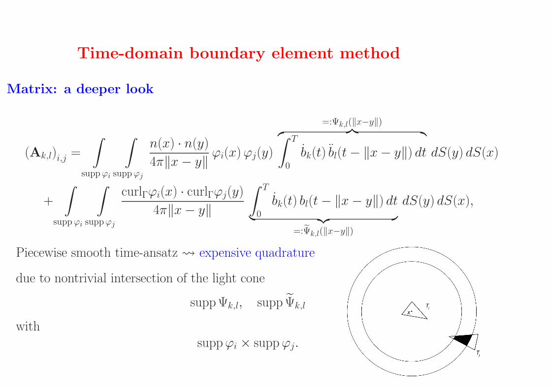
Matrix: a deeper look
(Ak,l)i,j =
∫
suppϕi
∫
suppϕj
n(x) · n(y)
4π‖x− y‖ϕi(x)ϕj(y)
=:Ψk,l(‖x−y‖)︷ ︸︸ ︷∫ T
0
bk(t) bl(t− ‖x− y‖) dt dS(y) dS(x)
+
∫
suppϕi
∫
suppϕj
curlΓϕi(x) · curlΓϕj(y)
4π‖x− y‖
∫ T
0
bk(t) bl(t− ‖x− y‖) dt︸ ︷︷ ︸
=:Ψk,l(‖x−y‖)
dS(y) dS(x),
Piecewise smooth time-ansatz expensive quadrature
due to nontrivial intersection of the light cone
suppΨk,l, supp Ψk,l
withsuppϕi × suppϕj.
Page 20
Time-domain boundary element method
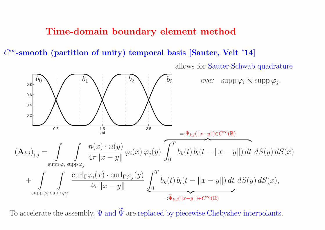
C∞-smooth (partition of unity) temporal basis [Sauter, Veit ’14]
0.5 1.5 2.5
0.2
0.4
0.6
0.8
t [s]
b0 b1 b2 b3
allows for Sauter-Schwab quadrature
over suppϕi × suppϕj.
(Ak,l)i,j =
∫
suppϕi
∫
suppϕj
n(x) · n(y)
4π‖x− y‖ϕi(x)ϕj(y)
=:Ψk,l(‖x−y‖)∈C∞(R)︷ ︸︸ ︷∫ T
0
bk(t) bl(t− ‖x− y‖) dt dS(y) dS(x)
+
∫
suppϕi
∫
suppϕj
curlΓϕi(x) · curlΓϕj(y)
4π‖x− y‖
∫ T
0
bk(t) bl(t− ‖x− y‖) dt︸ ︷︷ ︸
=:Ψk,l(‖x−y‖)∈C∞(R)
dS(y) dS(x),
To accelerate the assembly, Ψ and Ψ are replaced by piecewise Chebyshev interpolants.
Page 21
Time-domain boundary element method
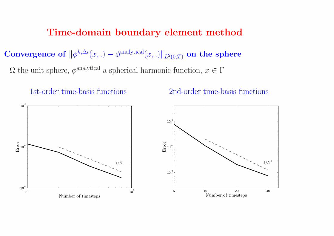
Convergence of ‖φh,∆t(x, .)− φanalytical(x, .)‖L2(0,T ) on the sphere
Ω the unit sphere, φanalytical a spherical harmonic function, x ∈ Γ
1st-order time-basis functions 2nd-order time-basis functions
101
102
10−3
10−2
10−1
1/N
Number of timesteps
Err
or
5 10 20 40
10−5
10−4
10−3
1/N 2
Number of timesteps
Err
or
Page 22
Time-domain boundary element method
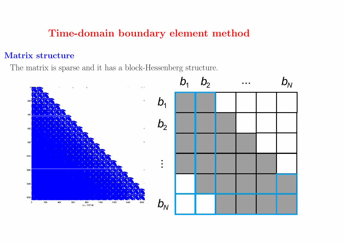
Matrix structure
The matrix is sparse and it has a block-Hessenberg structure.
Page 23
Parallel Time-Domain Boundary Element Methodfor 3-Dimensional Wave Equation
Outline
• Parallel fast BEM and applications
• Boundary integral formulation of sound-hard scattering
• Time-domain boundary element method
• Parallelization, preconditioning, numerical experiments
• Conclusion, outlook, references
Page 24
Parallelization, preconditioning, numerical experiments
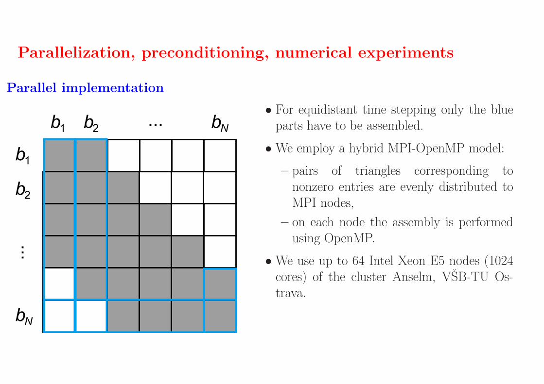
Parallel implementation
• For equidistant time stepping only the blueparts have to be assembled.
• We employ a hybrid MPI-OpenMP model:
– pairs of triangles corresponding tononzero entries are evenly distributed toMPI nodes,
– on each node the assembly is performedusing OpenMP.
• We use up to 64 Intel Xeon E5 nodes (1024cores) of the cluster Anselm, VSB-TU Os-trava.
Page 25
Parallelization, preconditioning, numerical experiments
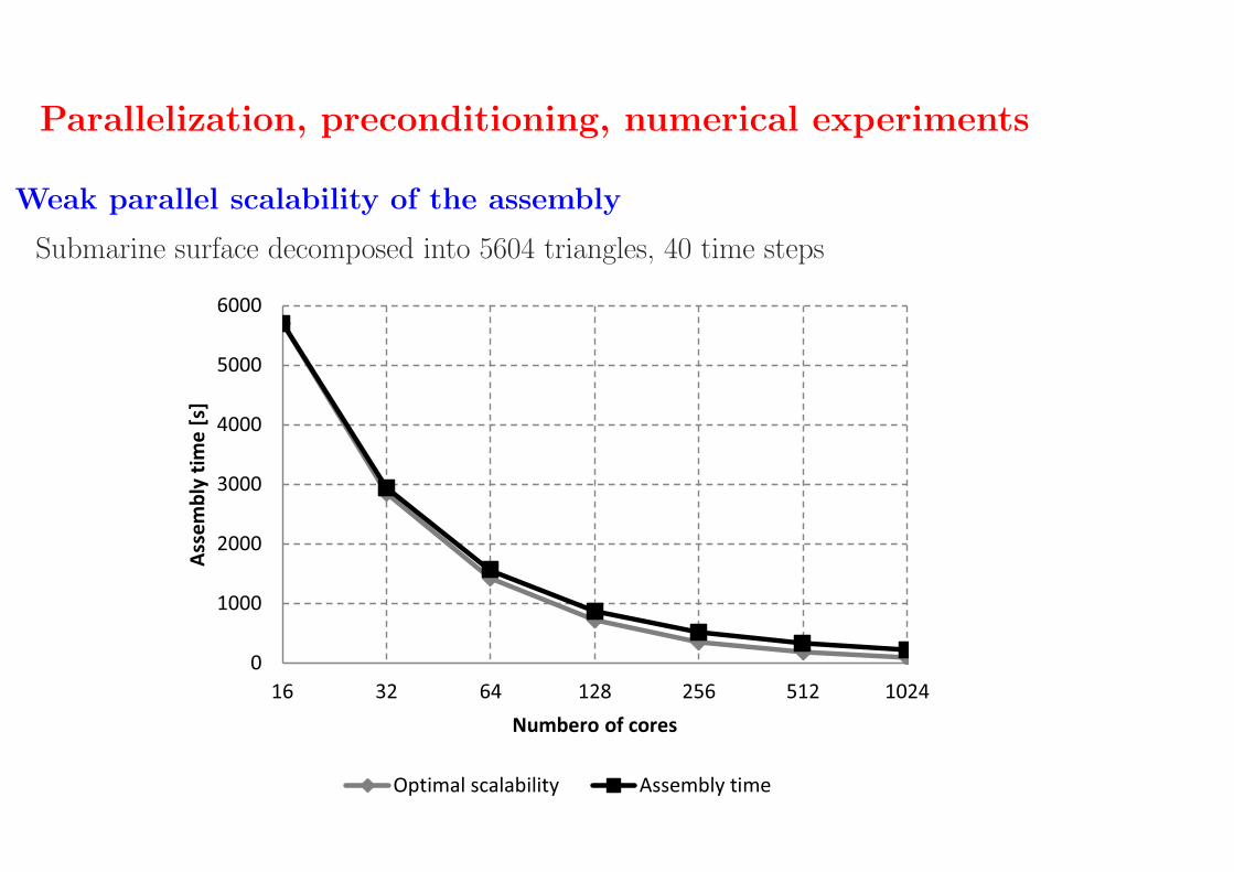
Weak parallel scalability of the assembly
Submarine surface decomposed into 5604 triangles, 40 time steps
Page 26
Parallelization, preconditioning, numerical experiments
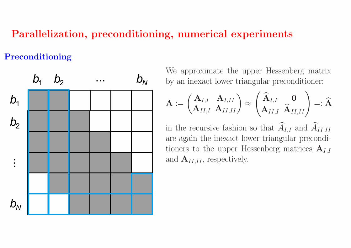
Preconditioning
We approximate the upper Hessenberg matrixby an inexact lower triangular preconditioner:
A :=
(AI,I AI,II
AII,I AII,II
)≈
(AI,I 0
AII,I AII,II
)=: A
in the recursive fashion so that AI,I and AII,II
are again the inexact lower triangular precondi-tioners to the upper Hessenberg matrices AI,I
and AII,II , respectively.
Page 27
Parallelization, preconditioning, numerical experiments
Numerical experiments
We compare convergence of preconditioned restarted GMRES, deflated GMRES, andflexible GMRES.
Page 28
Parallel Time-Domain Boundary Element Methodfor 3-Dimensional Wave Equation
Outline
• Parallel fast BEM and applications
• Boundary integral formulation of sound-hard scattering
• Time-domain boundary element method
• Parallelization, preconditioning, numerical experiments
• Conclusion, outlook, references
Page 29
Parallel Time-Domain Boundary Element Methodfor 3-Dimensional Wave Equation
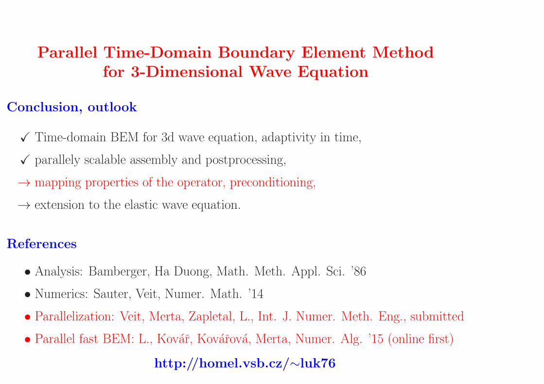
Conclusion, outlook
X Time-domain BEM for 3d wave equation, adaptivity in time,
X parallely scalable assembly and postprocessing,
→ mapping properties of the operator, preconditioning,
→ extension to the elastic wave equation.
References
• Analysis: Bamberger, Ha Duong, Math. Meth. Appl. Sci. ’86
• Numerics: Sauter, Veit, Numer. Math. ’14
• Parallelization: Veit, Merta, Zapletal, L., Int. J. Numer. Meth. Eng., submitted
• Parallel fast BEM: L., Kovar, Kovarova, Merta, Numer. Alg. ’15 (online first)
http://homel.vsb.cz/∼luk76