Work supported in part by US Department of Energy contract DE-AC02-76SF00515

Parameter Estimation and Confidence Regions in the Method of

Light Curve Simulations for the Analysis of Power Density

Spectra

Martin Mueller

Kavli Institute for Particle Astrophysics and Cosmology, SLAC National Accelerator

Laboratory, 2575 Sand Hill Road, Menlo Park, CA 94025, USA;

mmueller@slac.stanford.edu

and

Greg Madejski

Kavli Institute for Particle Astrophysics and Cosmology, SLAC National Accelerator

Laboratory, 2575 Sand Hill Road, Menlo Park, CA 94025, USA

ABSTRACT

The Method of Light Curve Simulations is a tool that has been applied to

X-ray monitoring observations of Active Galactic Nuclei (AGN) for the char-

acterization of the Power Density Spectrum (PDS) of temporal variability and

measurement of associated break frequencies (which appear to be an important

diagnostic for the mass of the black hole in these systems as well as their accretion

state). It relies on a model for the PDS that is fit to the observed data. The de-

termination of confidence regions on the fitted model parameters is of particular

importance, and we show how the Neyman construction based on distributions

of estimates may be implemented in the context of light curve simulations. We

believe that this procedure offers advantages over the method used in earlier re-

ports on PDS model fits, not least with respect to the correspondence between

the size of the confidence region and the precision with which the data constrain

the values of the model parameters. We plan to apply the new procedure to

existing RXTE and XMM observations of Seyfert I galaxies as well as RXTE

observations of the Seyfert II galaxy NGC 4945.

Subject headings: methods: data analysis — methods: statistical — X-rays:

galaxies

SLAC-PUB-13502May 2009

Published in the Astrophysical Journal

– 2 –

1. INTRODUCTION

The study of the temporal variability of the X-ray flux from accreting black holes has

revealed a complex behavior of the accretion flow (e.g. Mushotzky, Done & Pounds 1993;

Remillard & McClintock 2006). One widely applied tool for characterizing the variability

is the Power Density Spectrum (PDS). The shape of the broad-band PDS as well as the

location of identifiable features such as breaks and quasi-periodic oscillations provide the

observational constraints for physical models of the system that generates the variability. Of

particular interest is the apparent linear scaling between the high-frequency break timescale

and the black hole mass in these systems over many orders of magnitude (McHardy et al.

2004).

The analysis of the PDS of Active Galactic Nuclei (AGN) is complicated by the ques-

tion of how to assign uncertainties to the Fourier amplitudes measured from one observed

realization of what is presumed to be a stochastic process (Lawrence et al. 1987; McHardy

& Czerny 1987). A measure of the expected spread in the observed values is essential for

the correct interpretation of the Fourier spectrum. In addition, intrinsic properties of the

Fourier transform (red noise leak and aliasing), uneven sampling of the time series, and

measurement uncertainty in the count rate distort the spectrum; these effects need to be

corrected for when quantifying the shape of the broad-band spectrum. A method based on

Monte Carlo simulations to determine a reliable measure of the PDS uncertainties and to

account for these distortions was first proposed by Done et al. (1992). The main feature of

the method is the concept of simulating the possible range of realizations of the underlying

process and incorporating the shape-distorting effects of uneven sampling, red noise leak, and

aliasing. Uncertainties on the Fourier spectrum are determined using light curves generated

from a model for the PDS, and the level of agreement between the model and the data is

quantified by a χ2 fit statistic. By analogy to X-ray spectral fitting, the application of these

observational effects to the chosen model results in the “folded model”, which is then used

in the comparison to the observations.

Subsequent work by Uttley, McHardy & Papadakis (2002) (hereafter UMP02), incorpo-

rating the recommendations for the simulation of stochastic processes in Timmer & Koenig

(1995), led to a canonical method for the analysis of AGN X-ray light curves, obtained

mainly from RXTE and XMM-Newton. The process to be modeled is expressed in the form

of a parametric expression for the PDS; depending on the complexity of the model, a varying

number of adjustable parameters determine the shape and normalization of the model PDS.

In addition to the updated Monte Carlo simulations, the authors present detailed proce-

dures for the statistical evaluation of the model fit, i.e. the assignment of a goodness-of-fit

measure and the derivation of confidence regions on model parameters. The fit statistic,

– 3 –

which was dubbed the “rejection probability” by subsequent authors, is now different from

a standard χ2 statistic. This development toward a statistically more sophisticated tech-

nique was influenced by considerations about the resolution of the PDS, which often needs

to be compromised to satisfy the conditions under which the χ2 statistic may be used safely

(Papadakis & Lawrence 1993). This new method has found widespread applicability; the re-

sults reported in Markowitz et al. (2003) (hereafter M03), McHardy et al. (2004), Markowitz

(2005), McHardy et al. (2005), Uttley & McHardy (2005), McHardy et al. (2007), Sum-

mons et al. (2007), Arevalo, McHardy & Summons (2008), and Marshall, Ryle & Miller

(2008) are all based on it. Our initial report on the PDS of NGC 4945 (Mueller et al. 2004)

similarly took the published method and introduced some additional changes. (In contrast

to the above papers, Green, McHardy & Done (1999), Vaughan, Fabian & Nandra (2003),

Vaughan & Fabian (2003), and Awaki et al. (2005) implement Monte Carlo simulations for

the derivation of uncertainties on the PDS, but use the standard χ2 statistic for the model

fit.)

In the general case of fitting a model to a set of data, the derivation of best fit values of

the model parameters (called “point estimation” in statistics) involves the identification of

the location in parameter space at which the fit statistic attains an extremum1. These best fit

values are called “estimates”; the recipe for finding an estimate for a particular parameter is

called the “estimator”. Point estimates by themselves are of limited use. Instead, confidence

regions on the fitted model parameters characterize how well the data constrain the model,

and goodness-of-fit tests may be applied to test whether the chosen model is an adequate

description of the data and whether certain models are favored over others.

The definition of a confidence region is crucial to its proper interpretation. A confidence

region (with associated confidence level C) is a region in parameter space computed from

the measured data that has a probability C of containing the true set of parameter values.

In other words, if the measurement were repeated, a different confidence region would be

obtained for each data set, but a fraction C of them would enclose the (unknown) point

in parameter space on which the measured data are based. This of course assumes that

the model under consideration is the correct one; if a goodness-of-fit test indicates that the

chosen model is a bad description for the data, then confidence regions on its parameters are

of little value.

Confidence regions are often interpreted as expressing the precision with which the model

1The use of Monte Carlo simulations for the derivation of the folded model in the case of PDS fitting

results in a fit statistic that can not be expressed in closed form as a function of the parameters. Numerical

methods therefore need to be employed to search for the location of the extremum.

– 4 –

parameters may be determined given the data. In practice, for any given fitting procedure,

there are usually several plausible methods that produce regions with the required property

to make them confidence regions. A useful additional consideration is therefore whether the

size of the region that a chosen method returns depends appropriately on the measurement

uncertainties. Furthermore, the value of the fit statistic at the location of the best fit should

have no or only a weak influence on the size.2

We review some of the concepts of model fitting using the χ2 statistic in Section 2, and we

show how, in a simple toy model set-up, the ∆χ2 prescription for finding confidence regions

satisfies the consideration above. The “rejection probability” as a fit statistic is evaluated

on the same criteria in Section 3, and the strong dependence of the size of the confidence

region on the minimum rejection probability demonstrated. We then introduce the Neyman

construction based on simulated distributions of estimates in Section 4 as an alternative to

the use of the rejection probability. This paper does not present any actual results obtained

from the proposed method. However, we outline in Section 5 possible changes that may

occur if PDS model fits obtained using contours of constant rejection probability, including

our own work on NGC 4945, were re-examined using the Neyman construction. Section 6

summarizes the paper.

2. POINT ESTIMATION AND CONFIDENCE REGIONS USING THE χ2

STATISTIC

The most familiar fit statistic in Astrophysics is without a doubt the χ2 statistic. It

applies well to problems where the measured quantities are Gaussian distributed with known

uncertainties. Even in cases where that condition is not satisfied, the χ2 statistic can some-

times still yield useful parameter estimates. However, its main attraction lies in the ease with

which confidence regions on fitted parameters can be derived if the distributions are Gaus-

sians, namely through the concept of ∆χ2 (see e.g. Lampton, Margon & Bowyer 1976; Press

et al. 1992; Bevington & Robinson 2003). Any desired significance level 0 < α < 1 maps

onto a value of ∆χ2 such that, after determining the best fit values of the model parameters

by minimizing χ2, the region in parameter space bounded by the surface of constant ∆χ2

2By way of example, in a standard χ2 fit, under the assumption that the chosen model is the correct one

and that there are no systematic errors in the measurement, the minimum value of χ2 in a given fit is fully

determined by the ratio of the actual amount of statistical fluctuations in the data to the expected amount

and does therefore not depend on the size of the measurement uncertainties. In situations encountered in

practice, the conditions under which this is true are often violated to a certain degree, such that a small

influence on the size of the confidence region cannot be ruled out.

– 5 –

contains the true set of parameter values with a confidence C = 1 − α.

Let us illustrate the ∆χ2 procedure on a toy model setup to introduce additional notation

that we will refer back to in subsequent sections.

Let y be a physical variable that is expected to be proportional to a single indepen-

dent variable x. As part of an experiment, y is measured for a fixed set of non-equal xi

(i = 1, ..., N). The measurement is expected to result in Gaussian uncertainties on y, with

a constant standard deviation σ independent of i. Let {yi} (i = 1, ..., N) be the set of

measurements at the corresponding values xi.

We now wish to fit these data with a model y = k x. The χ2 fit statistic is then a

function of the one model parameter k and the set of observed values {yi} (all sums are over

i from 1 to N):

χ2(k, {yi}) =∑ (yi − kxi)

2

σ2. (1)

Minimizing χ2(k, {yi}) with respect to k yields the estimate k({yi}) and the minimum

value of the fit statistic χ2min({yi}):

k({yi}) =

∑

xi yi∑

x2i

(2)

and

χ2min({yi}) =

∑ (yi − kxi)2

σ2. (3)

Using these two equations, the expression for the change in χ2 as k is varied evaluates

to

∆χ2(k, {yi}) ≡ χ2(k, {yi}) − χ2min({yi}) =

∑

x2i

σ2(k − k({yi}))

2. (4)

To derive the 68% confidence region (i.e. the “1σ” uncertainties)3 around k({yi}) (sig-

nificance α = 0.32), we set ∆χ2(k, {yi}) = 1.00. The resulting region satisfies

3The term “1σ” is sometimes used to indicate the 68% confidence region even if the fit statistic is not

χ2. In such cases, the standard deviation of the distribution of the parameter may not have the same

interpretation, but the confidence regions parameterized by the confidence C are always well-defined.

– 6 –

|k − k({yi})| <σ

√

∑

x2i

. (5)

Since we assumed that the measured yi are in fact well-described by the model, then

each yi has to be drawn from a Gaussian distribution around the true value, i.e.

yi ∼ g(ktrue xi, σ), (6)

where g(a, b) is a Gaussian distribution with average a and standard deviation b, and ∼

denotes “drawn from.” The estimate k({yi}) is then drawn from the following probability

density function:

k({yi}) ∼ g

(

ktrue,σ

√

∑

x2i

)

. (7)

In other words, if the act of measuring the set {yi} is repeated many times, k({yi})

will differ from ktrue by less than σ/√

∑

x2i 68% of the time. It should now be immediately

obvious that the size of the confidence region (Equation 5) is such that in precisely those

68% of cases the confidence region includes ktrue, confirming what the confidence region was

designed to express about the experiment.

We have thus confirmed that in this simple setup, the ∆χ2 prescription produces inter-

vals for the model parameter k that satisfy the requirements of confidence intervals. Further-

more, it can be seen from Equation 5 that the size of the confidence interval is proportional to

the measurement uncertainty σ and independent of χ2min. We defer to existing publications

(specifically Lampton, Margon & Bowyer 1976) for the extension of these results to higher-

dimensional parameter spaces. We only wish to note here that the independence of the size

of the confidence region on χ2min is guaranteed through the independence of the distribution

of ∆χ2 on χ2min, as demonstrated in Lampton, Margon & Bowyer (1976, Appendix IV).

3. THE REJECTION PROBABILITY

The measurement of the level of agreement between the model and the observed data

in the method of light curve simulations in UMP02 relies on a statistic called by subsequent

authors the “rejection probability.” It is defined analogous to a p-value, with the rejection

probability being one minus the p-value of the measured χ2dist fit statistic. Differences in

– 7 –

best-fit rejection probability between different models are used to favor one model over the

others (e.g. a broken power law model compared to an unbroken power law model), and

regions in parameter space where the rejection probability is less than a certain value (e.g.

90%) are then taken as the confidence regions for the fitted model parameters.

3.1. Confidence Regions from Rejection Probability

By analogy to χ2 fitting, the UMP02 procedure for determining confidence regions is

equivalent to identifying the region in parameter space where χ2 is less than some critical

value. For the c% confidence region, this critical value is simply the c-th percentile of the

χ2 distribution with the appropriate number of degrees of freedom and is thus independent

of the minimum value of χ2 obtained in the fit. The reason why the authors do not rely on

percentiles of χ2 distributions for the determination of confidence regions is that the effective

number of degrees of freedom varies with position in parameter space. Deciding on the basis

of p-values whether a certain point in parameter space is included in the confidence region

is therefore more robust.

The region produced in this manner do have the required property to make them confi-

dence regions, i.e., they include the true value of the parameters with the desired probability.

However, their sizes depend strongly on the value of the fit statistic at the location of the

best fit. If the minimum rejection probability in a fit is just below 90%, the contours of 90%

rejection probability will be found fairly close around the best fit, leading to the erroneous

conclusion that the data lend themselves to the placement of very precise limits on the model

parameters. Note that a minimum rejection probability of 90% does not by itself indicate

a bad fit, since there is still a 10% chance of obtaining a fit as bad or worse due simply to

statistical fluctuations; we are therefore justified in searching for the confidence region asso-

ciated with the parameters of such a fit. Conversely, if the minimum rejection probability is

very low, the 90% contours will enclose a large area. Furthermore, if the minimum rejection

probability is above 90%, there will be no 90% confidence region at all.

We illustrate the inverse correlation between the minimum rejection probability and the

size of the resulting confidence region schematically in Figure 1. This behavior is apparent

in some of the published results (UMP02, M03, McHardy et al. 2007, Summons et al. 2007).

– 8 –

3.2. The Empirical Distribution of χ2dist

The calculation of the rejection probability relies on an approximate determination of

the empirical distribution of χ2dist: Since the effective number of degrees of freedom is a

function of the model parameters, the distribution is rightfully calculated separately for

each grid point in parameter space. However, the χ2dist values for the simulated Fourier

spectra are only calculated at their original grid point and are not the best fit values found

by performing the point estimation on each simulated spectrum (see e.g. Press et al. 1992,

Section 15.6).

The approximation was most likely introduced due to considerations about computing

time, because the minimization of χ2dist over the parameter space for the hundreds of simu-

lated spectra that are typically involved incurs a significant computational load. However,

given the advances in computer power since the original method was introduced, the reason

for the approximation may well have fallen away.

4. CONFIDENCE REGIONS AND GOODNESS-OF-FIT TEST USING

SIMULATED DISTRIBUTIONS OF ESTIMATES

We propose the following set of procedures, most importantly the Neyman construction

based on distributions of estimates for the derivation of confidence regions, as an alternative

to the use of the rejection probability for PDS model fits. The new method returns confidence

intervals whose size has the desired property of being independent of the value of the fit

statistic at the location of the best fit. Furthermore, it deals very naturally with biased

estimators4.

Throughout this section, it is assumed that the χ2dist fit statistic can be calculated for an

arbitrary point in parameter space through the use of simulated light curves. The procedures

are however not specific to the χ2dist fit statistic; any other statistic which attains an extremum

at the location of the best fit may be substituted for χ2dist.

4Biased estimators are estimators with an expectation value different from the true one. The k estimator

used in Section 2 is unbiased because its expectation value is ktrue (Equation 7). In more complicated

situations, such as the PDS fits under consideration here, one does not generally know a priori whether the

chosen estimators are biased or not.

– 9 –

4.1. Point Estimation

χ2dist may be used directly for point estimation, i.e. the estimates Θobs for the parameters

of the model used to describe the observed Fourier spectrum Pobs(ν) are the values of the

parameters at the grid point that minimize χ2dist. The estimates Θsim for any of the simu-

lated light curves (used further below) can be found similarly by substituting the simulated

spectrum in place of the observed spectrum and minimizing χ2dist over the parameter space.

4.2. Goodness-of-Fit and Hypothesis Testing

In order to test whether the minimum χ2dist value of the observed Fourier spectrum

signifies an acceptable fit, we use the simulations to determine the distribution from which

χ2dist is drawn. The null hypothesis is that the measured Fourier spectrum was in fact

produced by the model under consideration. Let Θbest be our best guess for the true values

of the parameters, i.e. the grid point closest to the center of the confidence region. (If the

estimators are unbiased, Θbest can be set equal to Θ.) For each of the simulated light curves

generated for Θbest, we record its best fit χ2dist (already found above in the determination

of the confidence region). The goodness-of-fit measure is then the familiar p-value of the

observed spectrum’s minimum χ2dist compared against this distribution of simulated χ2

dist

values. As such, it expresses the probability that a χ2dist value at least as high as the measured

one would be obtained by chance; a p-value smaller than the desired significance level (e.g.

5%) indicates that the null hypothesis can be rejected.

The reason for choosing Θbest over any other grid point is that the distribution of the

minimum values of χ2dist may depend on Θ. In standard χ2 fitting, the distribution of χ2

min is

independent of Θ, being in fact the χ2 distribution with the appropriate number of degrees of

freedom. In the framework of Fourier spectral fits, this independence appears to be broken,

such that the effective number of degrees of freedom is a function of the model parameters,

plausibly because the degree to which adjacent bins in the Fourier spectrum are correlated

depends on the amount of red noise leak (Mueller et al., in preparation). Using Θbest ensures

that the χ2dist distribution thus found approximates as closely as possible the one from which

the measured χ2dist was in fact drawn.

Note that, up to the approximation to the distribution of χ2dist used by UMP02, this

procedure is essentially equivalent to the calculation of the rejection probability. The p-value

is however only used as a goodness-of-fit measure and not for finding the confidence intervals.

If more than one model are under consideration to explain the measured data, e.g. when

one would like to test for the presence of a break in the Fourier spectrum, a decision statistic

– 10 –

for hypothesis testing needs to be set up. In the framework of the χ2dist fit statistic, the

difference in best fit χ2dist values between two models is a natural choice for such a statistic

(by analogy to the F-test for the χ2 fit statistic). The simulations can once again be used

to determine the distribution of this difference, from which the critical value corresponding

to a desired power of the test (“statistical significance”) may be derived. We do not further

elaborate on this procedure here, since the numbers and decisions involved depend on a

balance between the sensitivity and specificity of the test that can only be calculated using

actual simulations.

4.3. Confidence Regions

We implement the Neyman construction (Neyman 1937) based on simulated distribu-

tions of estimates to find confidence limits on model parameters: Let C be the desired

confidence, e.g. 68% or 90%, and Θobs the estimates for the observed Fourier spectrum as

found above. Consider now an arbitrary grid point in parameter space, Θtrial. Using the sim-

ulated light curves generated for that point, we can determine the distribution of estimates

Θsim and derive a region in parameter space that encloses a fraction C of them. If Θobs is

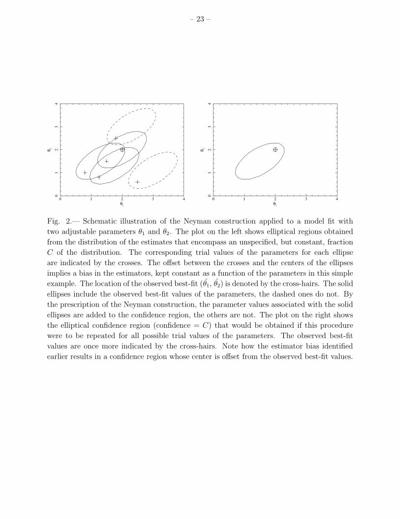
inside that region, Θtrial is included in the confidence region, otherwise it is not. Figure 2

shows this graphically in an imagined two-parameter model fit.

It is easy to see that the size of the confidence regions thus obtained is independent of the

value of the minimum χ2dist; no information about the measured data enters the calculation of

the distribution of estimates, and only the estimates Θobs are used in the subsequent mapping

of the confidence region. Also, the distribution of estimates, being a measure of the possible

range of parameter values that might be observed given the design of the measurement,

will be broad or narrow depending on the uncertainties in the observed Fourier spectrum.

Therefore, the size of the confidence region will scale with the uncertainties, preserving the

intended interpretation that the size of the confidence region expresses the precision with

which fitted model parameters can be determined.

As a consequence of using distributions of estimates in the Neyman construction, biased

estimators will be corrected, and the region returned by the algorithm has the required

property of enclosing the true values of the parameters with probability C. In principle, if

any of the estimators are strongly biased, Θobs might lie outside the confidence region. The

confidence region is however always more meaningful in the determination of probable values

of model parameters than a (possibly biased) point estimate.

Note also that the shape of the region enclosing the fraction C of all simulations may be

– 11 –

freely chosen by the user. This freedom is intrinsic to the Neyman construction. However,

in order to obtain the tightest possible constraints on the parameters, the smallest region

should be used.

A complication arises out of the limitation of being able to evaluate χ2dist only on a grid

in parameter space. The distributions of the estimates are therefore composed of finite-size

volume elements centered on each grid point. The use of smoothed approximations to the

empirically derived distributions can eliminate this step-wise behavior; for a one-dimensional

parameter space, if the distribution of the estimate is sharply peaked, one might use a

Gaussian fit and determine from the fitted average and standard deviation whether the trial

point lies inside the confidence interval. Similarly, in two dimensions, the use of ellipses

fitted to the empirical distribution to enclose the required fraction of simulated estimates

might be appropriate.

Let us illustrate the procedure of finding confidence regions using simulated distributions

of estimates on the toy model introduced in Section 2. The difference to the procedure

described above is that the estimate k can be found analytically and does not rely on a

grid search using simulations. However, let us suppose that simulations were set up for this

simple problem. We use Equation 2 to calculate kobs for the measured data {yi}. Let ktrial

be an arbitrarily chosen real number, for which we want to determine whether it is inside

the confidence interval. Using simulations with ktrial as the “true” parameter value (i.e.

randomizations of the observations as given by Equation 6), we would then find (Equation

7) that the probability density function of the estimates for this trial value is given by

g(ktrial, σ/√

∑

x2i ), i.e. a Gaussian distribution centered on ktrial. (In this toy model, the

distribution of the estimates is translationally invariant under changes in ktrial; this feature is

not expected in general.) The smallest interval enclosing 68% of the simulations is comprised

of the values within one standard deviation from ktrial, and by the prescription of the method

ktrial is included in the confidence region if and only if

|ktrial − kobs| <σ

√

∑

x2i

, (8)

thus recovering the confidence region in Equation 5.

4.3.1. The Confidence Interval for the Model Normalization

The model to be fit to the data usually includes an overall normalization factor that

carries through to the model prediction as a multiplicative factor. In this situation, the

– 12 –

derivation of confidence intervals on the model normalization can be simplified. In practice,

simulations need only be done once for an arbitrary normalization, since the model prediction

and uncertainties for any other normalization may be calculated simply by scaling. (For a

discussion of the complications introduced by measurement uncertainties, see Appendix A.1.)

For point estimation, the best fit normalization at any point in parameter space5 can easily be

found, either analytically or through a numerical search. This procedure is unchanged from

UMP02 (section 4.2). The estimates for the remaining parameters, either for the measured

data or for any of the simulated spectra that may be substituted for it, are then once again

the values of the parameters at the grid point in the remaining parameter space where χ2dist

attains a minimum.

For the derivation of confidence regions, we again wish to determine whether a certain

grid point in parameter space, with normalization Ntrial and remaining parameters Θtrial,

is included at a given significance level. Let N0 be the original normalization with which

the light curves at Θtrial were simulated, and f0(N , Θ) the corresponding probability density

function of the estimate distribution with its dependence on the normalization estimate N

and the estimates of the remaining model parameters Θ. Because of the multiplicative nature

of the model normalization, this distribution becomes scale-invariant along the N axis (see

Appendix A), such that if a different normalization had been used to simulate those light

curves, the distribution would simply be an appropriately scaled version of f0(N , Θ).

The point estimation on the observed Fourier spectrum defines the location of the best

fit, given by (Nobs, Θobs). We now determine the region R in the (N , Θ) space that encloses

the required fraction C of the estimate distribution (e.g. 68%). Now consider the line in

parameter space along which Θ = Θobs, i.e. the line parallel to the N axis that passes through

the best fit. This line either intersects the boundary of R in a finite number of points, or else

no intersection points exist. The region R is in most cases convex, such that there are either

zero or two intersection points. We will only consider these two cases here; the procedure is

easily generalized to non-convex regions that may result in additional intersection points.

In the case of zero intersection points, (Ntrial, Θtrial) is excluded from the confidence

region for all values of Ntrial. In the other case, let us denote the values of the normalization

at the two intersection points by N0,low and N0,high. Because of the scale-invariance of the

estimate distribution, these values are proportional to the original normalization N0, such

that, for any other normalization N that could have been used to generate the light curves,

5The parameter space now under consideration excludes the model normalization as a parameter, due to

its special treatment.

– 13 –

Nlow(N) =N

N0

N0,low (9)

and

Nhigh(N) =N

N0

N0,high. (10)

The condition for (Ntrial, Θtrial) to be included in the confidence region now reduces to

whether the observed value of the normalization is located between these two bounds, i.e.

Nlow(Ntrial) ≤ Nobs ≤ Nhigh(Ntrial), (11)

which is equivalent to the condition on Ntrial

N0

Nobs

N0,high

≤ Ntrial ≤ N0

Nobs

N0,low

. (12)

In summary, the estimate distribution found from light curves simulated at Θtrial, with

normalization N0, may be used to derive the bounds N0,low and N0,high, from which the

limits on Ntrial (for a given Θtrial) may be calculated. The confidence region in the full (N ,

Θ) parameter space finally may be mapped out by repeating the procedure for different

values of Θtrial.

5. DISCUSSION

Applying the criterion whether the procedure for determining confidence regions returns

regions whose size scales appropriately with the uncertainties in the data, we believe that

the Neyman construction based on simulated distributions of estimates offers a viable and

advantageous alternative to the use of the rejection probability. While neither UMP02 nor

the authors of the subsequent papers utilizing the method make specific claims regarding

the statistical properties of the regions obtained, anyone not familiar with the data analysis

at a sufficient level of detail will tend to interpret the quoted uncertainties on the best-fit

values of the model parameters as indicative of the precision with which the data constrain

those values.

We wish to stress however that this does not imply that previously reported results

are inherently flawed. The confidence limits on break frequencies and power law indices for

– 14 –

AGN PDS fits may turn out to be different under the application of the new method, but

it remains to be seen whether any of these changes are large enough to substantially change

the interpretation of the observations. Specifically, we do not expect that the linear scaling

between break timescale and black hole mass (McHardy et al. 2004) will be affected even if

the confidence intervals on some of the data points were to be modified.

It is likely that the precision with which the break frequencies for Fairall 9, NCG 4151

(both from M03), and MCG-6-30-15 (UMP02) have been reported is too optimistic. Simi-

larly, the confidence regions for the peak frequencies of the Lorentzians in the fit to the PDS

of Ark 564 may be too small, especially considering that even a small increase in the size of

the confidence contour in a plot where the axes are the logarithms of the peak frequencies

(Figure 9 in their paper) has a disproportionate effect on the uncertainties on the frequencies

themselves. On the other hand, some break frequencies may in fact be better determined

with current data than reported in the literature. Examples of fits where the minimum

rejection probability turned out to be particularly low include NGC 5548 and NGC 3516

(M03).

A related issue is the use of contours of constant rejection probability as confidence

limits on combinations of parameters, such as the ratio of break frequencies (Figure 11 in

McHardy et al. 2005 and Figure 6 in Uttley & McHardy 2005). Limits on this ratio are

used as key pieces of evidence to motivate the association of the AGNs under consideration

(NGC 3227 and MCG–6-30-15) with the analogue of the high/soft accretion state in galactic

black hole X-ray binaries. Given that the confidence regions were derived using the rejection

probability, the quoted confidence values with which certain ranges of ratios are excluded in

those reports may or may not in fact be supported by the data. We do not expect that the

use of the new method will alter the general direction of these results, i.e. that the ratio of

break frequencies in these AGN is likely to be higher than expected for the low/hard state,

but a re-analysis of the observations focusing on the doubly-broken power law model might

be warranted. The calculation of the statistical significance with which the model where

the ratio of these break frequencies is fixed at a value of 30 may be rejected in favor of the

original model where both break frequencies are allowed to vary forms an additional test on

these data. If both of these lines of evidence produce mutually consistent results, the case

for the classification of these AGN as analogues of galactic X-ray binaries in the high/soft

state will be strengthened.

On the question of the statistical significance of breaks in the PDS of AGN, we believe

that additional work is needed to make the values that have been reported more secure.

Table 5 in M03 lists the quantity ∆σ that was designed to express the increase in likelihood

of the fit once a break is added to the PDS model. It is however not clear from the description

– 15 –

whether ∆σ was calculated using the rejection probability or the underlying χ2dist values. As

outlined in Section 4.2, the χ2dist fit statistic does lend itself to the formulation of such a

hypothesis test. A validation of critical values of differences in χ2dist and their corresponding

statistical significances will be required. This includes using the simulated light curves to

calculate type I and type II errors (rate of false positives and false negatives) or, equivalently,

the specificity and sensitivity of the hypothesis test. As far as we are aware, the amount

and quality of data needed to effect a reliable detection of a break at a significance level of

5%, say, is an unanswered question. A systematic investigation in this area, using both real

and simulated data, might uncover general considerations that would be invaluable for the

design of future observatories for AGN timing research.

The Monte Carlo method for calculating folded models to include observational effects

may have applications outside of PDS fits to AGN X-ray light curves. In particular, the as-

sociated procedure of finding confidence limits on fitted parameters using simulated estimate

distribution could be used for X-ray or γ-ray spectral fits in the low counts-per-bin limit,

where the discrete nature of the Poisson process becomes important. The study of the PDS

of galactic X-ray binaries may benefit from an application of the Monte Carlo method as

well. The shorter time scales for characteristic variations and the extensive archive of X-ray

observations allow for a much more detailed investigation into the shape of the broad-band

variability spectrum, including the direct observation of independent realizations of the un-

derlying process (e.g. Pottschmidt et al. 2003; Done & Gierlinski 2005). The measurement

of the distribution of power in individual frequency bins is of particular interest in this case.

Competing physical models for the variability in these sources predict distinctive properties

of the stationarity and degree of stochasticity of the process underlying the observations

(e.g. Poutanen & Fabian 1999; Maccarone & Coppi 2002; Minutti & Fabian 2004; Uttley,

McHardy & Vaughan 2005; Zycki & Maciolek-Niedzwiecki 2005). Adopting the Monte Carlo

simulations for the analysis of galactic X-ray binaries, specifically the comparison between

predicted and observed distributions of the Fourier amplitude, may lead to tests of certain

elements of these models. Furthermore, tools beyond the PDS for the investigation of these

kinds of stochastic processes, such as the bispectrum (Vaughan & Uttley 2007), are more

sophisticated in their treatment of the underlying variability process, but they will also con-

tinue to, at least for a while, produce results that are not as validated in their interpretation

as those derived from standard Fourier analysis. Monte Carlo simulations will likely re-

main essential for the important comparison of these tools to the PDS; a solid statistical

foundation is in turn essential for these simulations.

– 16 –

6. CONCLUSION

Evaluated by the criterion whether the sizes of the confidence regions express the pre-

cision with which the data constrain the model parameters, we have shown that the use of

simulated distributions of estimates (Section 4.3) is preferable to the rejection probability

(Section 3.1). Confidence regions determined from the latter do have the required property

of enclosing the true values of the parameters with the given probability, but their size is

highly variable depending on the minimum value of the fit statistic at the location of the best

fit. The method based in the former is computationally more intensive, but is the only way

known to us to derive meaningful uncertainties on fitted model parameters in the absence of

a better-understood fit statistic.

The end products of the application of the set of procedures in Section 4.1 through

4.3 to the observations of an AGN are the best fit values of the parameters for the model-

dependent description of the PDS, the associated confidence limits, and the goodness-of-fit

of the model (p-value of the minimum χ2dist). Depending on the nature of the investigation,

more sophisticated statistical tests may be employed to test different hypotheses against

the same data set, or to quantify the observed variations in the parameter values between

different AGN.

We are in the process of applying the new method to the RXTE observation of the

Seyfert II galaxy NGC 4945 for which we reported first results in Mueller et al. (2004) and

plan to re-analyze the existing archival RXTE and XMM-Newton observations of Seyfert I

galaxies with the updated procedure. While we don’t expect the conclusions drawn from the

analysis of these observations to change significantly, this will put the investigation into the

shape of the PDS in AGN on a statistically more solid foundation and make the interpretation

of the results easier.

ACKNOWLEDGMENTS

We are indebted to the anonymous referee for much valued input on an earlier version

of this publication, especially concerning the development of the analysis method based on

the rejection probability. We would furthermore like to acknowledge Alex Markowitz for

providing the initial impetus for the critical examination of the rejection probability, and

Chris Done and Piotr Zycki for the ongoing collaboration on the analysis of the NGC 4945

observations. We also thank Jeff Scargle, and especially Frank Porter, for many fruitful

discussions on statistical techniques and their expertise on the associated terminology. This

research was supported in part by the U.S. Department of Energy Contract DE-AC02-

– 17 –

76SF00515 to the SLAC National Accelerator Laboratory.

A. THE SCALE-INVARIANCE OF THE ESTIMATE DISTRIBUTION FOR

THE MODEL NORMALIZATION

The special treatment of the model normalization in the derivation of confidence regions

relies on a property of the estimate distribution under the conditions mentioned in the text

(Section 4.3.1), namely that the normalization carries through to the model prediction as a

multiplicative factor.

Let N0 be the normalization (hereafter called the “input normalization”) that was used

to generate a set of light curves at an arbitrary point in parameter space Θtrial, and let

{Pin(νi)} be the Fourier spectrum of one of them, where νi are the frequencies over which

the spectrum is measured. Additionally, let (Nin, Θin) be the estimates for this light curve

that were found as part of the procedure to determine the estimate distribution (see Section

4.3 for details). Because the normalization is an overall multiplicative factor in the generation

of these light curves, the {Pin(νi)} values are proportional to N0.

The model to be fit to these data can be written as P (ν, N, Θ) = N Pr(ν, Θ), where

N is the model normalization and Pr(ν, Θ) the function describing the dependence of the

model on the remaining parameters Θ. The folded model at the point in parameter space

given by N and Θ is summarized in two variables for each frequency bin: the average power

Psim(νi, N, Θ) and the standard deviation ∆Psim(νi, N, Θ) (for details, see Section 4.2 in

UMP02). Both of these scale with N :

Psim(νi, N, Θ) = N Psim,r(νi, Θ), (A1)

and

∆Psim(νi, N, Θ) = N ∆Psim,r(νi, Θ), (A2)

where Psim,r(νi, Θ) and ∆Psim,r(νi, Θ) constitute the folded model for N = 1. The fit

statistic

χ2dist(N, Θ, {Pin(νi)}) =

∑

i

(

Pin(νi) − N Psim,r(νi, Θ)

N ∆Psim,r(νi, Θ)

)2

(A3)

– 18 –

is invariant under changes in the input normalization N0 → η N0 (η > 0) if the same

multiplicative factor is applied to the model normalization N . As a consequence, since Nin

and Θin are the estimates for this simulated light curve for η = 1, then (η Nin) and Θin would

have been the estimates if the original normalization had been different by a factor η. This

applies to all simulated spectra; therefore the distribution of the estimates (Nin, Θin) will be

scale-invariant along the N axis: Let f0(N , Θ) be the estimate distribution for the original

input normalization N0 (i.e. η = 1). For any other value of η, the estimate distribution is

then

f(N , Θ) =1

ηf0

(

N

η, Θ

)

. (A4)

Note that the above does not require that the normalization be uncorrelated with the

other model parameters. The invariance of the fit statistic is preserved even if such correla-

tions exist.

A.1. Influence of Measurement Uncertainties

In the context of PDS model fits, the measurement uncertainties in the light curve man-

ifest themselves as an additional noise component in the Fourier spectrum (Poisson level).

The scaling of the model prediction with the normalization factor is only approximate in this

case, since the Poisson level is constant and does not scale with the model normalization.

However, the intrinsic variability in the light curve by design usually dominates over the

Poisson level. The confidence interval on the model normalization derived while ignoring

this complication is therefore expected to approximate closely the more correct one that

would be obtained through the usual prescription of simulating light curves with different

normalizations and deriving the distribution of the estimates in each case.

A.2. Applicability to PDS with Logarithmically Averaged Power

In the canonical method of UMP02, Psim(νi) is actually the average of the logarithm of

the periodogram power, which is motivated by the considerations in Papadakis & Lawrence

(1993). The logarithm of the model normalization N therefore enters the model prediction as

an additive constant, while the uncertainties ∆Psim(νi), being standard deviations on what

are now logarithmic power values whose spread is unaffected by the model normalization,

are independent of N . The estimate distribution is then translationally invariant along the

– 19 –

log N axis, and the expression for the bounds on Ntrial turns out to be the same as for the

linear case (Equation 12).

Note however that different numerical values for these bounds may be obtained depend-

ing on whether the estimate distribution is expressed as a function of N or log N . The shape

and extent of the region R encompassing the desired fraction of the estimate distribution

may vary; the smallest such region for example will in general be different depending on the

choice of variables. In a complete description of the analysis method, it will be important

to state which variable was used.

REFERENCES

Arevalo, P., McHardy, I. M., Summons, D. P. 2008, MNRAS, 388, 211

Awaki, H., Murakami, H., Leighly, K. M., Matsumoto, C., Hayashida, K., Grupe, D. 2005,

ApJ, 632, 793

Bevington, P. R., Robinson, D. K. 2003, Data Reduction and Error Analysis for the Physical

Sciences, 3rd edition, McGraw-Hill

Done, C., Gierlinski, M. 2005, MNRAS, 364, 208

Done, C., Madejski, G. M., Mushotzky, R. F., Turner, T. J., Koyama, K., Kunieda, H. 1992,

ApJ, 400, 138

Green, A. R., McHardy, I. M., Done, C. 1999, MNRAS, 305, 309

Lampton, M., Margon, B., Bowyer, S. 1976, ApJ, 208, 177

Lawrence, A., Watson, M. G., Pounds, K. A., Elvis, M. 1987, Nature, 325, 694

Maccarone, T. J., Coppi, P. S. 2002, MNRAS, 336, 817

Markowitz, A. 2005, ApJ, 635, 180

Markowitz, A. et al. 2003, ApJ, 593, 96 (M03)

Marshall, K., Ryle, W. T., Miller, H. R. 2008, ApJ, 677, 880

McHardy, I. M., Arevalo, P., Uttley, P., Papadakis, I. E., Summons, D. P., Brinkmann, W.,

Page, M. J. 2007, MNRAS, 382, 985

McHardy, I., Czerny, B. 1987, Nature, 325, 696

– 20 –

McHardy, I. M., Gunn, K. F., Uttley, P., Goad, M. R. 2005, MNRAS, 359, 1469

McHardy, I. M., Papadakis, I. E., Uttley, P., Page, M. J., Mason, K. O. 2004, MNRAS, 348,

783

Minutti, G., Fabian, A. C. 2004, MNRAS, 349, 1435

Mueller, M., Madejski, G., Done, C., Zycki, P. 2007, in Kaaret, P., Lamb, F. K., Swank,

J. H., eds., X-Ray Timing 2003: Rossi and Beyond, American Institute of Physics,

Melville, NY, 714, 190

Mushotzky, R. F., Done, C., Pounds, K. A. 1993, ARA&A, 31, 717

Neyman, J. 1937, Philosophical Transactions of the Royal Society of London, Series A,

Mathematical and Physical Sciences, 236, 333

Papadakis, I. E., Lawrence. A. 1993, MNRAS, 261, 612

Pottschmidt, K. et al. 2003, A&A, 407, 1039

Poutanen, J., Fabian, A. C. 1999, MNRAS, 306, L31

Press, W. H., Teukolsky, S. A., Vetterling, W. T., Flannery, B. P. 1992, Numerical Recipes,

Cambridge University Press, Cambridge

Remillard, R. A., McClintock, J. E. 2006, ARA&A, 44, 49

Summons, D. P., Arevalo, P., McHardy, I. M., Uttley, P., Bhaskar, A. 2007, MNRAS, 378,

649

Timmer, J., Koenig, M. 1995, A&A, 300, 707

Uttley, P., McHardy, I. M. 2005, MNRAS, 363, 586

Uttley, P., McHardy, I., Papadakis, I. 2002, MNRAS, 332, 231 (UMP02)

Uttley, P., McHardy, I. M., Vaughan, S. 2005, MNRAS, 359,345

Vaughan, S., Fabian, A. C. 2003, MNRAS, 341, 496

Vaughan, S., Fabian, A. C., Nandra, K. 2003, MNRAS, 339, 1237

Vaughan, S., Uttley, P. 2007, in Cohen, L. ed., Noise and Fluctuations in Photonics, Quan-

tum Optics, and Communications, Proc. SPIE, 6603, 660314

– 21 –

Zycki, P., Niedzwiecki, A. 2005, MNRAS, 359, 308

This preprint was prepared with the AAS LATEX macros v5.2.

– 22 –

050

100

reje

ctio

n pr

obab

ility

(%)

model parameter k

68%

conf. reg.68%

Fig. 1.— Schematic plot illustrating the dependence of the size of the confidence region

on the minimum value of the rejection probability. The solid and dashed lines are stylized

representations of the behavior of the rejection probability as a function of a model parameter

k for fits to two different data sets. Both fits return the same estimate for k, but due to

statistical fluctuations, the fit indicated by the solid line results in a significantly lower

minimum rejection probability. The procedure for determining the 68% confidence interval

on k for each fit is indicated by the dotted lines, showing the projection of the intersection

points between the line of 68% rejection probability and the respective parabola onto the

k axis. Even though this is only a schematic representation, and the detailed behavior of

the rejection probability as a function of any of the parameters in a real fit may be more

complicated, the negative correlation between the size of the confidence region and the

minimum value of the rejection probability is expected in general.

– 23 –

0 1 2 3 4

01

23

4

θ 2

θ1

0 1 2 3 4

01

23

4

θ 2θ1

Fig. 2.— Schematic illustration of the Neyman construction applied to a model fit with

two adjustable parameters θ1 and θ2. The plot on the left shows elliptical regions obtained

from the distribution of the estimates that encompass an unspecified, but constant, fraction

C of the distribution. The corresponding trial values of the parameters for each ellipse

are indicated by the crosses. The offset between the crosses and the centers of the ellipses

implies a bias in the estimators, kept constant as a function of the parameters in this simple

example. The location of the observed best-fit (θ1, θ2) is denoted by the cross-hairs. The solid

ellipses include the observed best-fit values of the parameters, the dashed ones do not. By

the prescription of the Neyman construction, the parameter values associated with the solid

ellipses are added to the confidence region, the others are not. The plot on the right shows

the elliptical confidence region (confidence = C) that would be obtained if this procedure

were to be repeated for all possible trial values of the parameters. The observed best-fit

values are once more indicated by the cross-hairs. Note how the estimator bias identified

earlier results in a confidence region whose center is offset from the observed best-fit values.