RESEARCH ARTICLE 10.1002/2015WR017295 Parameter estimation and prediction for groundwater contamination based on measure theory S. A. Mattis 1 , T. D. Butler 2 , C. N. Dawson 1 , D. Estep 3 , and V. V. Vesselinov 4 1 Institute for Computational Engineering and Sciences, University of Texas at Austin, Austin, Texas, USA, 2 Department of Mathematical and Statistical Sciences, University of Colorado Denver, Denver, Colorado, USA, 3 Department of Statistics, Colorado State University, Fort Collins, Colorado, USA, 4 Computational Earth Science Group, Earth and Environmental Sciences Division, Los Alamos National Laboratory, Los Alamos, New Mexico, USA Abstract The problem of groundwater contamination in an aquifer is one with many uncertainties. Prop- erly quantifying these uncertainties is essential in order to make reliable probabilistic-based predictions and decisions regarding remediation strategies. In this work, a measure-theoretic framework is employed to quantify uncertainties in a simplified groundwater contamination transport model. Given uncertain data from observation wells, the stochastic inverse problem is solved numerically to obtain a probability measure on the space of unknown model parameters characterizing groundwater flow and contaminant transport in an aquifer, as well as unknown model boundary or source terms such as the contaminant source release into the environment. This probability measure is used to make predictions of future contaminant concen- trations and to analyze possible remediation techniques. The ability to identify regions of small but nonzero probability using this method is illustrated. 1. Introduction Contamination of groundwater aquifers is a significant problem in many locations around the world [R€ ugner et al., 2006; National Research Council, 2013]. In many instances, there may be various remedia- tion strategies for reducing contamination levels that are economically viable and technically sound. However, determination of an optimal remediation strategy is complicated by many factors. Most reme- diation strategies are subject to governmental budget constraints [National Research Council, 1999, 2013], and the actual outcomes of various plausible remediation strategies are often uncertain for a vari- ety of reasons, e.g., due to the limited information in characterizing the past, current, and future nature and extent of contaminants in the environment. This causes substantial uncertainties in future concen- trations predicted from models under different remediation scenarios. There are many additional uncer- tainties related to the contaminant transport and fate including the identification of the magnitude, size, and duration of the contaminant release in the environment. Further complicating the problem of mak- ing accurate predictions are inherent uncertainties in the geological, hydrological, and biogeochemical conditions of the affected aquifer due to limited characterization data. Consequently, in order to make useful predictions of concentrations of a contaminant, its effect on the environment, and to best plan for remediation, quantifying uncertainties impacting the contaminant transport and fate is essential. The process for quantifying uncertainties affecting real-world decisions regarding complex physical proc- esses requires the fusion of data-driven and model-driven techniques to incorporate what little informa- tion is known. There has been a great deal of work regarding the development of theoretical and computational frame- works for contaminant remediation incorporating uncertainties in the parameters and models [see Bolster et al., 2009; Agostini et al., 2009a, 2009b; Argent et al., 2009; Tartakovsky, 2007; Jordan and Abdaal, 2013; National Research Council, 1999]. Often, there is uncertainty in the underlying flow and transport models and model inadequacy studies can improve results [Ye et al., 2004; Beven and Westerberg, 2011]. There have been many attempts to incorporate model and prediction uncertainty into the decision-making pro- cess for remediation [Caselton and Luo, 1992; Hipel and Ben-Haim, 1999; Bolster et al., 2009; Reeves et al., 2010; Harp and Vesselinov, 2013; O’Malley and Vesselinov, 2014]. It is common to characterize the uncer- tainties in groundwater contamination models probabilistically [Delhomme, 1979; Dagan, 1982; Wagner Key Points: Apply measure-theoretic framework to inverse problem for contaminant transport Identify and estimate both high- and low-probability parameter events Quantify uncertainties in predictions for remediation strategies Correspondence to: S. A. Mattis, [email protected]Citation: Mattis, S. A., T. D. Butler, C. N. Dawson, D. Estep, and V. V. Vesselinov (2015), Parameter estimation and prediction for groundwater contamination based on measure theory, Water Resour. Res., 51, 7608–7629, doi:10.1002/ 2015WR017295. Received 24 MAR 2015 Accepted 24 AUG 2015 Accepted article online 28 AUG 2015 Published online 18 SEP 2015 V C 2015. American Geophysical Union. All Rights Reserved. MATTIS ET AL. PARAMETER ESTIMATION AND PREDICTION 7608 Water Resources Research PUBLICATIONS
Transcript
RESEARCH ARTICLE10.1002/2015WR017295
Parameter estimation and prediction for groundwatercontamination based on measure theoryS. A. Mattis1, T. D. Butler2, C. N. Dawson1, D. Estep3, and V. V. Vesselinov4
1Institute for Computational Engineering and Sciences, University of Texas at Austin, Austin, Texas, USA, 2Department ofMathematical and Statistical Sciences, University of Colorado Denver, Denver, Colorado, USA, 3Department of Statistics,Colorado State University, Fort Collins, Colorado, USA, 4Computational Earth Science Group, Earth and EnvironmentalSciences Division, Los Alamos National Laboratory, Los Alamos, New Mexico, USA
Abstract The problem of groundwater contamination in an aquifer is one with many uncertainties. Prop-erly quantifying these uncertainties is essential in order to make reliable probabilistic-based predictions anddecisions regarding remediation strategies. In this work, a measure-theoretic framework is employed toquantify uncertainties in a simplified groundwater contamination transport model. Given uncertain datafrom observation wells, the stochastic inverse problem is solved numerically to obtain a probability measureon the space of unknown model parameters characterizing groundwater flow and contaminant transport inan aquifer, as well as unknown model boundary or source terms such as the contaminant source releaseinto the environment. This probability measure is used to make predictions of future contaminant concen-trations and to analyze possible remediation techniques. The ability to identify regions of small but nonzeroprobability using this method is illustrated.
1. Introduction
Contamination of groundwater aquifers is a significant problem in many locations around the world[R€ugner et al., 2006; National Research Council, 2013]. In many instances, there may be various remedia-tion strategies for reducing contamination levels that are economically viable and technically sound.However, determination of an optimal remediation strategy is complicated by many factors. Most reme-diation strategies are subject to governmental budget constraints [National Research Council, 1999,2013], and the actual outcomes of various plausible remediation strategies are often uncertain for a vari-ety of reasons, e.g., due to the limited information in characterizing the past, current, and future natureand extent of contaminants in the environment. This causes substantial uncertainties in future concen-trations predicted from models under different remediation scenarios. There are many additional uncer-tainties related to the contaminant transport and fate including the identification of the magnitude, size,and duration of the contaminant release in the environment. Further complicating the problem of mak-ing accurate predictions are inherent uncertainties in the geological, hydrological, and biogeochemicalconditions of the affected aquifer due to limited characterization data. Consequently, in order to makeuseful predictions of concentrations of a contaminant, its effect on the environment, and to best plan forremediation, quantifying uncertainties impacting the contaminant transport and fate is essential. Theprocess for quantifying uncertainties affecting real-world decisions regarding complex physical proc-esses requires the fusion of data-driven and model-driven techniques to incorporate what little informa-tion is known.
There has been a great deal of work regarding the development of theoretical and computational frame-works for contaminant remediation incorporating uncertainties in the parameters and models [see Bolsteret al., 2009; Agostini et al., 2009a, 2009b; Argent et al., 2009; Tartakovsky, 2007; Jordan and Abdaal, 2013;National Research Council, 1999]. Often, there is uncertainty in the underlying flow and transport modelsand model inadequacy studies can improve results [Ye et al., 2004; Beven and Westerberg, 2011]. Therehave been many attempts to incorporate model and prediction uncertainty into the decision-making pro-cess for remediation [Caselton and Luo, 1992; Hipel and Ben-Haim, 1999; Bolster et al., 2009; Reeves et al.,2010; Harp and Vesselinov, 2013; O’Malley and Vesselinov, 2014]. It is common to characterize the uncer-tainties in groundwater contamination models probabilistically [Delhomme, 1979; Dagan, 1982; Wagner
Key Points:� Apply measure-theoretic framework
to inverse problem for contaminanttransport� Identify and estimate both high- and
low-probability parameter events� Quantify uncertainties in predictions
Citation:Mattis, S. A., T. D. Butler, C. N. Dawson,D. Estep, and V. V. Vesselinov (2015),Parameter estimation and predictionfor groundwater contamination basedon measure theory, Water Resour. Res.,51, 7608–7629, doi:10.1002/2015WR017295.
Received 24 MAR 2015
Accepted 24 AUG 2015
Accepted article online 28 AUG 2015
Published online 18 SEP 2015
VC 2015. American Geophysical Union.
All Rights Reserved.
MATTIS ET AL. PARAMETER ESTIMATION AND PREDICTION 7608
and Gorelick, 1987; Abbaspour et al., 1997; Keating et al., 2010], where a probability distribution is associ-ated with each parameter separately. Representing probabilities in high dimensions can be challenging,but some recent methods have increased computational efficiency [Tonkin and Doherty, 2009; Laloy andVrugt, 2012].
We present a recently developed measure-theoretic framework for the formulation and solution to a physi-cally meaningful stochastic inverse problem for quantifying uncertainties in a physics-based model [Breidtet al., 2011; Butler et al., 2012; Butler and Estep, 2013; Butler et al., 2014; T. Butler et al., Solving stochasticinverse problems using sigma-algebras on contour maps, 1407.3851, 2014]. A computational algorithm isdescribed in detail and applied to a mathematical model for groundwater contamination. The inverse solu-tion is a probability measure that is consistent with the unique solution in the space of parameter equiva-lence classes defined by the physics-based map from parameters to data. By consistent, we mean thatpropagation of the probability measure through the computational model exactly reproduces the probabil-ity measure on the data space. These equivalence classes can be identified as generalized contours in theoriginal parameter space. We demonstrate how the probability measure can be used to identify andapproximate the probability of failure events for various remediation strategies in terms of reducing futurecontaminant levels below the maximum concentration limit (MCL).
The use of generalized contours in the formulation and solution of the stochastic inverse problem is quitedifferent from other approaches that have appeared in the literature. A complete literature review is infeasi-ble, so we limit the comparison below to popular approaches focusing on similar applications. Bayesian andGeneralized Likelihood Uncertainty Estimation (GLUE) approaches have proven to be among the most pop-ular approaches for quantifying uncertainties in hydrologic models and environmental problems [see Freerand Beven, 1996; Leube et al., 2012; Nowak et al., 2010; Troldborg et al., 2010; Vrugt et al., 2008; Beven andFreer, 2001]. The Bayesian and GLUE approaches replace the map from uncertain parameters to observa-tions defined by the physics-based model with a statistical map called the likelihood function. After specify-ing a prior distribution on the parameters, the objective is to interrogate a posterior distribution defined interms of the likelihood and prior distributions often by using a Markov Chain Monte Carlo (MCMC) sam-pling. In other words, the inverse problem is formulated in terms of a statistical problem involving the fit ofmodel outputs to data, and typical objectives are either to produce a set of samples generated from theposterior distribution or to determine the parameters of maximum likelihood. The maximum likelihood canoften be reinterpreted as the minimum of a misfit functional which defines a so-called ‘‘regularized’’ solutionto the inverse problem (e.g., see the sequence of papers [Carrera and Neuman, 1986a,b,c] for the methods,algorithms, and applications of this idea). In regularization, one seeks to minimize a misfit functional definedusing both residual errors along with a ‘‘penalty’’ term. The covariances of the likelihood and prior distribu-tions in a Bayesian formulation can often be used to define the norms used for the residual errors and pen-alty term, respectively. Since the regularized solution is the solution to an optimization problem,interpretation of the obtained results often involve some type of sensitivity analysis [see Carrera et al., 2005;Carrera and Neuman, 1986a; Mayer et al., 2002]. By design, the misfit functionals in regularizationapproaches and the related posterior distributions in Bayesian approaches have completely different con-tour structures than the generalized contours of the physics-based map between model parameters andobservational data. The implication is that the solutions to the regularization and Bayesian approaches solvea different inverse problem and have completely different interpretations than what is obtained by themeasure-theoretic formulation and solution of the inverse problem.
The paper is organized as follows. In section 2, we describe the contaminant transport model, physicaldomain, and model parameters that are the focus of this work. In section 3, we summarize the measure-theoretic framework and computational algorithm used in the rigorous probabilistic analysis of uncertain-ties. In section 4, we provide numerical results demonstrating this probabilistic analysis on the contaminanttransport model. A low-dimensional problem is solved to illustrate the effect of the underlying geometrydefined by the choice of quantities of interest on the solution to the stochastic inverse problem. A higher-dimensional stochastic inverse problem is then solved and used to quantify uncertainties in both modeland source parameters. The solution of the higher-dimensional stochastic inverse problem is used to makepredictions about contaminant plumes when no remediation is performed and for a variety of remediationstrategies. We focus the analysis of predictions specifically on reducing contaminant levels below the MCL.Concluding remarks follow in section 5.
Water Resources Research 10.1002/2015WR017295
MATTIS ET AL. PARAMETER ESTIMATION AND PREDICTION 7609
2. Contaminant Transport Model and Parameters
Contaminant transport in groundwater aquifers is a complex process and its modeling is associated with agreat deal of underlying uncertainty. We demonstrate the benefit of quantifying uncertainties using themeasure-theoretic framework in section 4.4 by comparing the resulting probabilistic predictions to thoseobtained from an uninformed predictive analysis. In order to explore the entire set of possible parametersand identify regions of high probability in an uninformed way, typically, a large number of forward model sol-utions are computed. In order to do this efficiently, we use a relatively simple analytical model with manysources of uncertainty [Wang and Wu, 2009] as a forward model. We note that using a more complicatedmodel presents no theoretical difficulties in the measure-theoretic approach while the practical approximationissues can be addressed directly using adaptive sampling based on computable error estimates/bounds (T.Butler et al., Solving stochastic inverse problems using sigma-algebras on contour maps, 1407.3851, 2014), butthis is beyond the scope of this work. In section 3.3, we provide a general description of the convergence anderror analysis in the measure-theoretic approach and compare to the more traditional sampling methodsusing posterior distributions obtained via a Bayesian formulation.
Some assumptions are made about the model domain and setup in order to simplify the model as shownin Figure 1. We assume that the domain is infinite in the horizontal (x-y) plane and semiinfinite in the verti-cal (z) direction, and that the region of contaminant release (the contamination source) is a rectangular box,and the volumetric mass released per unit time (the mass flux) is uniform within the source at a given time.The groundwater flow field is steady and uniform in the horizontal direction. The contaminant undergoesfirst-order decay, accounting for a variety of geochemical processes that might be reducing the contami-nant concentration (e.g., first-order chemical reactions) [Petrucci et al., 1993]. We assume there is no contam-inant in the domain at the initial time, and the aquifer hydraulic conductivity and porosity arehomogeneous throughout the domain. The resulting contaminant transport is modeled using a three-dimensional advection-dispersion-reaction equation:
@C@t
1u@C@x
2uax@2C@x2
2uay@2C@y2
2uaz@2C@z2
1dC5I=n; (1)
where C ½ML23� is the contaminant concentration. The model parameters ax, ay, and az ½L� are the dispersiv-ities in the x, y, and z directions, respectively, u ½LT21� is the pore groundwater flow velocity along the x axis,d ½T21� is the first-order constant for decay, n ½L3=L3� is the porosity of the aquifer, and I ½ML23T21� is thecontaminant mass flux. The source I is defined by
Iðx0; y0; z0; tÞ5I0; x2
12
xs < x0 < x112
xs; y 212
ys < y0 < y112
ys; z0 < z0 < z1;
t0 < t < t1
0; otherwise;
8>>><>>>:
(2)
where I0 is a given constant. The source parameters defining I include the location of the center of the con-taminant source at x (m), y (m), and z0 (m) and the size of the source xs (m), ys (m), and z1 (m) (in the x, y,and z directions, respectively). The remaining source parameters are t0 (year) the initial time of the source,t1 (year) the final time of the source, and f ðkg=yearÞ the contaminant flux within the source. Under thegiven assumptions, there exists an analytical solution:
MATTIS ET AL. PARAMETER ESTIMATION AND PREDICTION 7610
where j is a time scaling factor fordispersivity. If j 5 1, there is notime scaling for dispersivity. Ifj > 1, the dispersivity scales withthe travel time. Scaling of the dis-persivity for the case of transport inporous geologic media has beenfrequently observed in field hydro-geologic studies [Neuman, 1990;Gelhar et al., 1992; Schulze-Makuch,2005].
By equation (1), the source I andthe solution Cðx; y; z; tÞ, there are alarge number of parameters thatdetermine the concentration of thecontaminant at a given point in thespace-time domain even for this
simplified model. They can be divided into two categories: source and transport parameters. Sourceparameters characterize the contaminant release into the aquifer. Transport parameters represent theunderlying transport processes in the aquifer. The measure-theoretic framework for quantifying uncer-tainties formulates the stochastic inverse problem with respect to a parameter domain containing all ofthese model and source parameters. Generally these parameters are not known exactly or even esti-mated. In practice, the available information consists of observations of contaminant concentrations atspecific points in space-time. However, under reasonable assumptions about the source and the proper-ties of the aquifer, intervals in which the parameter values are contained may be determined orestimated.
3. Measure-Theoretic Framework for Uncertainty Quantification
This section summarizes the mathematical methodology and numerical methods for a measure-theoreticframework for stochastic inverse problems for physics-based maps as formulated by Breidt et al. [2011],Butler et al. [2012], Butler and Estep [2013], Butler et al. [2014], and T. Butler et al. (Solving stochastic inverseproblems using sigma-algebras on contour maps, 1407.3851, 2014). Below, we emphasize the core deter-ministic forward and inverse maps at the heart of all the computations involving uncertainties modeledwith probability measures. In order to make these ideas less abstract, we connect the notation and conceptsto the model described above.
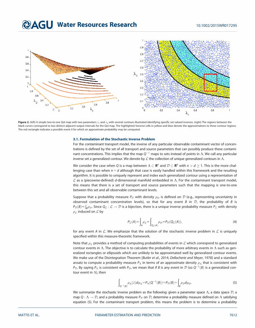
We let K denote the space of possible (input) parameters for the model (including source parameters)and Q be a map from the parameter space K to the output space D : 5QðKÞ. Here D representscontaminant concentrations given by the map Q defined by evaluating Cðx; y; z; tÞ at specific points inspace-time that depend implicitly on the choice of parameters. The components of Q are referred to as‘‘quantities of interest’’ (QoI) and Q is called the QoI map. In an idealized case, Q would be a bijection(i.e., a one-to-one and onto map) between K and D. This idealized situation is rarely the case evenwhen K and D have the same dimension. Typically, there is a set of points in K that are mapped to thesame point in D by Q, i.e., the map Q21 is set-valued. For example, increasing the porosity while decreas-ing the contaminant mass flux may result in no difference in observed contaminant concentrations.Moreover, the dimension of D is often less than that of K, which implies that the set-valued inverses aredefined by a collection of lower-dimensional manifolds embedded in K that we call generalized con-tours. In either case, it is impossible to assign a distinct parameter to a distinct output datum. We illus-trate this idea in the left plot in Figure 2. Putting this in the stochastic setting where parameters and/ordata are random variables does not change the fundamental issue that the map Q21 is set-valued. Solv-ing the stochastic inverse problem involves computing a probability measure on the original parameterspace K, given a probability measure on D and the set-valued map Q21 that maps to generalized con-tours in K.
Figure 1. Configuration of contaminant transport model.
Water Resources Research 10.1002/2015WR017295
MATTIS ET AL. PARAMETER ESTIMATION AND PREDICTION 7611
3.1. Formulation of the Stochastic Inverse ProblemFor the contaminant transport model, the inverse of any particular observable contaminant vector of concen-trations is defined by the set of all transport and source parameters that can possibly produce these contami-nant concentrations. This implies that the map Q21 maps to sets instead of points in K. We call any particularinverse set a generalized contour. We denote by L the collection of unique generalized contours in K.
We consider the case when Q is a map between K � Rn and D � Rd with n > d � 1. This is the more chal-lenging case than when n 5 d although that case is easily handled within this framework and the resultingalgorithm. It is possible to uniquely represent and index each generalized contour using a representation ofL as a (piecewise-defined) d-dimensional manifold embedded in K. For the contaminant transport model,this means that there is a set of transport and source parameters such that the mapping is one-to-onebetween this set and all observable contaminant levels.
Suppose that a probability measure PD with density qD is defined on D (e.g., representing uncertainty inobserved contaminant concentration levels), so that for any event B in D, the probability of B isPDðBÞ5
ÐBqD. Since QL : L ! D is a bijection, there is a unique inverse probability measure PL with density
qL induced on L by
PLðAÞ5ð
AqL5
ðQLðAÞ
qD5PDðQLðAÞÞ; (4)
for any event A in L. We emphasize that the solution of the stochastic inverse problem in L is uniquelyspecified within this measure-theoretic framework.
Note that qL provides a method of computing probabilities of events in L which correspond to generalizedcontour events in K. The objective is to calculate the probability of more arbitrary events in K such as gen-eralized rectangles or ellipsoids which are unlikely to be approximated well by generalized contour events.We make use of the Disintegration Theorem [Butler et al., 2014; Dellacherie and Meyer, 1978] and a standardansatz to compute a probability measure PK in terms of an approximate density qK that is consistent withPD. By saying PK is consistent with PD, we mean that if B is any event in D (so Q21ðBÞ is a generalized con-tour event in K), then
ðQ21ðBÞ
qKðkÞdlK5PKðQ21ðBÞÞ5PDðBÞ5ð
BqDdlD: (5)
We summarize the stochastic inverse problem as the following: given a parameter space K, a data space D, amap Q : K! D, and a probability measure PD on D, determine a probability measure defined on K satisfyingequation (5). For the contaminant transport problem, this means the problem is to determine a probability
Figure 2. (left) A simple two-to-one QoI map with two parameters k1 and k2 with several contours illustrated identifying specific set-valued inverses. (right) The regions between theblack curves correspond to two distinct adjacent output intervals for the QoI map. The highlighted Voronoi cells in yellow and blue denote the approximations to these contour regions.The red rectangle indicates a possible event A for which an approximate probability may be computed.
Water Resources Research 10.1002/2015WR017295
MATTIS ET AL. PARAMETER ESTIMATION AND PREDICTION 7612
measure on the transport and source parameters such that mapping this probability measure through the modelproduces the same probability measure as the one defined on the observable contaminant concentrations.
3.2. Numerical Solution to the Stochastic Inverse ProblemSuppose the probability density function qD associated with PD is known. Let fDkgM
k51 be a partition of D,and let pk be the probability of Dk. Let A be an event in K. We thus have the approximation
ðQðAÞ
qDdlD �X
Dk�QðAÞpk: (6)
Let fkðjÞgNj51 be a collection of N points in K, which implicitly defines an n-dimensional Voronoi tessellation fV j
gNj51 associated with the points. For example, given k 2 K; k 2 Vk if kðkÞ is the closest kðjÞ to k. Using the implic-
itly defined Voronoi tessellation and the partitioning ofD, Algorithm 1 can be used to calculate the probabilityq̂K;j associated with the implicitly defined Voronoi cell V j . We illustrate the steps of Algorithm 1 using the sim-ple quadratic QoI map from a 2-D parameter space (n 5 2) to a 1-D data space (d 5 1) shown in Figure 2. Inpractice, we only construct the samples in step 1 of Algorithm 1 and the Voronoi tessellation of step 2 is implic-itly defined by the set of samples from step 1. However, for pedagogical reasons, it is easier to visualize theremaining steps of the algorithm using the explicit Voronoi tessellation as shown in the right plot of Figure 2.Step 3 of the algorithm simply defines which data value is associated with each Voronoi cell. Step 4 defines apartitioning of the data space which corresponds to a unique collection of generalized contour events in K. Inthe right plot of Figure 2, the regions between the black curves represent the exact contour events correspond-ing to two subintervals from a possible partition ofD. The probabilities associated with these regions are deter-mined by qD as indicated in step 5 of Algorithm 1. Steps 6 and 7 are used to identify which Voronoi cells areused to approximate the exact contour events implicitly defined by step 4. In the right plot of Figure 2, we useyellow and blue highlighting to distinguish which collections of Voronoi cells are identified as approximatingthe two contour events with boundaries given by the black curves. Note that steps 8 and 9 of Algorithm 1determine the probability of each individual Voronoi cell according to the ansatz discussed above, where thevolume is determined in step 8 and the ansatz is applied in step 9. Note that in steps 5 and 8 in Algorithm 1, wemust approximate integrals. The computation of step 8 uses Monte Carlo integration in high-dimensionalspaces. We then approximate the probability of any event A � K using a counting measure
PKðAÞ �XkðjÞ2A
q̂K;j: (7)
Thus, we obtain an approximation to the probability measure on K that solves the stochastic inverse prob-lem as described above and satisfies equation (5). In the right plot of Figure 2, we consider A defined as theregion interior to the red rectangle and the probabilities of the Voronoi cells have all been determined. Bysimply identifying the samples in A and summing the probabilities associated with these samples toapproximate P(A), we can reinterpret this counting measure approximation as a type of Monte Carloapproximation to PKðAÞ.
Algorithm 1. Numerical Approximation of Inverse Probability Density
1. Choose points fkðjÞgNj51 2 K.
2. Denote the associated Voronoi tessellation fV jgNj51 � K.
3. Evaluate Qj5QðkðjÞÞ for all kðjÞ; j51; . . . ;N.
4. Choose a partitioning of D; fDkgMk51 � D.
5. Compute pk �Ð
DkqDdlD; for k51; . . . ;M.
6. Let Ck5fjjQj 2 Dkg for k51; . . . ;M.
7. Let Oj5fkjQj 2 Dkg; for j51; . . . ;N.
8. Let Vj be the approximate measure of V j , i.e., Vj �ðV j
dlðV jÞ for j51; . . . ;N.
9. Set q̂K;j5ðVj=Xi2COj
ViÞpOj ; j51; . . . ;N.
Water Resources Research 10.1002/2015WR017295
MATTIS ET AL. PARAMETER ESTIMATION AND PREDICTION 7613
3.3. Computational Complexity and Error AnalysisAs described in section 1, the inverse problems formulated in the measure-theoretic framework and Bayes-ian frameworks are fundamentally different, which complicates any direct comparisons between the solu-tion methods. However, if we assume there are no hyperparameters used in the definitions of the priordistributions for the Bayesian formulation, then the solutions to either problem formulation are (different)probability measures on the (same) parameter space. If the goal of generating samples from the Bayesianposterior distribution is to approximate probabilities (i.e., measures) of events, then it may at least be possi-ble to compare the cost of approximating the solutions to within some specified accuracy with sample-based approaches. A rigorous analysis of the computational cost for numerical methods for either problemformulation is not the focus of this work. Here we summarize the basic components of a convergence anderror analysis to describe how such comparisons of the computational cost associated with using Algorithm 1can be made to the computational cost of using a standard Monte Carlo sampling scheme to numericallyapproximate posterior distributions using a Bayesian framework. For a more thorough explanation of thetheory and proofs related to convergence and error analysis of Algorithm 1, we direct the interested reader toButler et al. [2014] and T. Butler et al. (Solving stochastic inverse problems using sigma-algebras on contourmaps, 1407.3851, 2014).
Using a standard Monte Carlo sampling scheme in a Bayesian framework to estimate the posteriorensures independence and can easily be used to provide estimates of probabilities of events written asexpected values. The convergence of the estimates of probabilities of events is then subject to the well-known Central Limit Theorem. As described in Butler et al. [2014], Algorithm 1 can be interpreted as aMonte Carlo approximation to probabilities of events. The key to the convergence results in Butler et al.[2014] is to understand the approximation of events using results from stochastic geometry that rely onthe Strong Law of Large Numbers, which is a key result used in proving the Central Limit Theorem.Thus, it may be possible to compare the rates of convergence for either method using similar statisticaltools.
It may also be possible to compare the cost of using an MCMC approach to sample the posterior distribu-tion for a Bayesian formulation to an importance sampling approach used to place more samples inregions of high probability within Algorithm 1. This is a key interpretation that would lead to what werefer to as ‘‘adaptive sampling’’ algorithms within the measure-theoretic approach and is the subject offuture work.
There remains the issue of the effect of numerical error on the computed solution. The effect of numericalerror in solving a computational model pollutes the QoI samples in both the measure-theoretic and Bayes-ian framework. However, the measure-theoretic framework allows for a straightforward error analysis wherethe effect of this deterministic error on the estimated probabilities of events can be quantified. The key tothis part of the error analysis is to use computable a posteriori error estimates (e.g., using an adjoint to theoriginal model) as a way to identify possible ‘‘mischaracterization’’ of an output sample (i.e., incorrectlydetermining Oj in step 7 of Algorithm 1). This type of error analysis for a fixed computational model isunusual in a Bayesian framework, and to the authors knowledge, has not been carried out.
Addressing these issues in more detail and within the numerics would require a detailed description ofadaptive sampling approaches, adjoint models, and a posteriori error estimates, which is beyond the scopeof this work. We avoid issues of error in the numerics below by using the analytical solution and a suffi-ciently large number of samples so that all asymptotic bounds on statistical error can be considerednegligible.
4. Numerical Results
Given a set of source and transport parameters, equation (3) can be used to calculate the concentration ofthe contaminant at points within the domain of interest. We use the open-source software package ModelAnalysis and Decision Support (MADS) (http://mads.lanl.gov; https://gitlab.org/monty/MADS) developed atLos Alamos National Laboratory, which makes such calculations computationally efficient. Accurate approxi-mations to the transport solutions are obtained using GNU Science Library (GSL) subroutines. The open-source software package called BET (https://github.com/UT-CHG/BET) developed by the authors is used tocompute the probability measure.
Water Resources Research 10.1002/2015WR017295
MATTIS ET AL. PARAMETER ESTIMATION AND PREDICTION 7614
When Q : K � Rn ! D � Rd is piecewise differentiable, the implicit function theorem implies that the rankof the Jacobian of Q is at most min n; df g. This motivates the definition of geometrically distinct (GD) QoIdefined as a set of QoI whose Jacobian is full rank [Butler et al., 2014]. Clearly, there exists at most n GD QoI.Given m � n possible QoI, we may be able to choose several d � n subsets of the possible QoI that satisfythe property of being GD. Given two distinct sets of QoI that are GD does not imply that the solutions tothe inverse problem computed from either set will be the same. The quality of a solution to the inverseproblem is affected by how the map Q skews events mapped between L and D. This is similar to the condi-tion number of a square matrix. A full analysis on the effect of the choice of QoI and the skewness on theprobability measure PK is beyond the scope of this work, and we direct the interested reader to Butler et al.[2015] for a more thorough discussion. However, we demonstrate in section 4.2 how the choice of GD QoIcan have a large influence on the structure of the inverse probability measure for a low-dimensional param-eter example where the number of possible QoI is larger than the number of parameters. In the higher-dimensional numerical example of section 4.3, the number of available QoI from the experiment is strictlyless than the number of uncertain parameters, so we simply use all of the available QoI. The problem ofhow to choose an optimal GD subset from a proposed set of QoI by quantifying the skewness is the subjectof on-going research. In section 4.3, we demonstrate how to analyze a probability measure in high dimen-sions. In section 4.4, we use the probability measure on the higher-dimensional parameter space to makepredictive inferences and analyze various remediation strategies.
4.1. ConfigurationThe region of interest for the solution to equation(1) is shown in Figure 3. The region contains 10wells labeled w1 through w10. The x-y coordinatesof these wells are shown in Table 1. Wells w1–w7are monitoring wells from which measurements ofthe concentration of the contaminant are taken.Wells w8, w9, and w10 are points of compliance(PoC). Contaminant concentrations in the PoC arerequired to be below a threshold known as the MCL(EPA, http://water.epa.gov/drink/contaminants). Forthis study, the MCL is assumed to be 25 mg/kg. Themeasured concentrations of the contaminant areknown at t51 year in the monitoring wells w1–w7and are listed in Table 1. This model setup and data
Figure 3. The domain of interest for the model problem with wells w1–w10 shown. The red rectangle indicates the potential locations forthe center of the source.
Table 1. Spatial Locations of Wells and Observed ContaminantConcentrations C at t51 year Taken From Studies in Harp andVesselinov [2012]a
are taken from studies in Harp and Vesselinov [2012].The contaminants in the PoC are assumed unknownat time t51 year.
In the numerical results below, we define a proba-bility measure PD on D in terms of a probabilitydensity qD in the following way. We assume thatany measured datum is subject to uncertainty withknown error bounds for each component of the QoImap such that each component of the true datumis within these bounds. With no additional assump-tions on the structure of the uncertainty within D,this implies that the true vector-valued datum existswithin a hyperbox centered on this measureddatum and contained in D. In each example, wespecify the size of the hyperbox relative to the sizeof a circumscribing hyperbox D. In order not to biasresults too closely to the specific contour mappingto the measured datum, we take qD to be the uni-form density on this hyperbox.
4.2. QoI Influence on the Inverse Probability MeasureWe first consider the case where there are only three unknown parameters: the x coordinate of the sourcex, the y coordinate of the source y, and the contaminant source flux f. Probabilities can be visualized effec-tively for such a low-dimensional problem. Table 2 shows the possible intervals of the unknown parametersand the fixed values of the other parameters that are assumed known. The specified intervals for x, y, and fdefine the parameter domain K5½210; 1460�3½1230; 1930�3½0:1; 100� where we let k5ðx; y; f Þ (i.e.,k15x; k25y, and k35f ). Suppose that the QoI are the concentrations of the contaminant in wells w1–w7 after1 year of contamination, and let qiðkÞ be the concentration in well wi for i51; 2; . . . ; 7 for a given value ofk 2 K. Let q̂i denote the measured concentration in well wi for i51; 2; . . . ; 7 shown in Table 1. To more clearlydemonstrate the influence of the choice of QoI on PK, we focus on using different sets of two GD QoI and pres-ent some representative examples below.
Suppose qi and qj are the chosen pair of GD QoI so that QðkÞ5½qiðkÞ; qjðkÞ�T for all k 2 K and D5QðKÞ. Wedefine a probability measure on D following the steps described above. We first define a hyperbox (in this
Table 2. Ranges for Unknown Parameters and Fixed Values forKnown Parameters for Low-Dimensional Inverse StochasticSensitivity Analysis
Unknown Parameters Min. Max.
Source coordinate x (m) 210 1460Source coordinate y (m) 1230 1930Contaminant source flux f (kg/year) 0.1 100
Known Parameters Value
Porosity n 0.1Flow angle h (8) 0Pore velocity u (m/year) 16Source size xs (m) 250Source size ys (m) 250Source location z0 (m) 0Source size z1 (m) 1Reactive decay k (1/year) 0.01Longitudinal dispersivity ax (m) 70Transverse horizontal dispersivity ay (m) ax=10Transverse vertical dispersivity az (m) ax=100Dispersivity time-scaling factor j 1.2Initial source time t0 (year) 0End source time t1 (year) 20
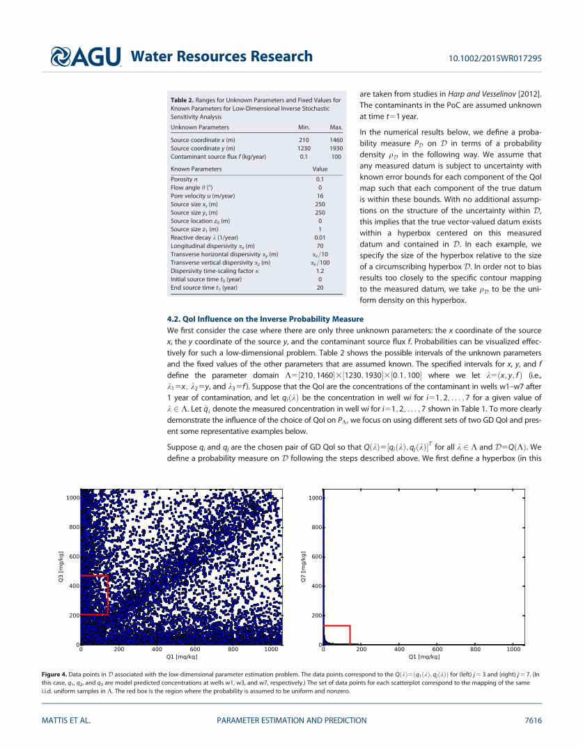
Figure 4. Data points in D associated with the low-dimensional parameter estimation problem. The data points correspond to the QðkÞ5ðq1ðkÞ; qjðkÞÞ for (left) j 5 3 and (right) j 5 7. (Inthis case, q1, q2, and q3 are model predicted concentrations at wells w1, w3, and w7, respectively.) The set of data points for each scatterplot correspond to the mapping of the samei.i.d. uniform samples in K. The red box is the region where the probability is assumed to be uniform and nonzero.
Water Resources Research 10.1002/2015WR017295
MATTIS ET AL. PARAMETER ESTIMATION AND PREDICTION 7616
case, a rectangle since D � R2) centered at ½q̂i; q̂j� of dimensions ð0:3qiðKÞÞ3ð0:3qjðKÞÞ (see Figure 4 forsome representative plots). We apply N553104 independent identically distributed (i.i.d.; in this case, theyare uniform) samples kðjÞ
n oN
j51in Algorithm 1 to approximate PK.
Figure 5. Computed 2-D marginal probabilities for the (top row) x and y coordinates of the source, (middle row) y coordinate of the source and contaminant source flux f, and (bottom row)x coordinate of the source and contaminant source flux f obtained by solving the stochastic inverse problem using QðkÞ5ðq1ðkÞ; qjðkÞÞ for (left column) j 5 3 and (right column) j 5 7.
Water Resources Research 10.1002/2015WR017295
MATTIS ET AL. PARAMETER ESTIMATION AND PREDICTION 7617
For low-dimensional QoI spaces such as these, itis possible to analyze scatter plots of the QoI toinfer the geometric relationship of the data withrespect to the parameters and determine whichQoI map skews events mapped between K andD the most. We show some representativeQoI scatter plots in Figure 4 for ðq1ðkÞ; q3ðkÞÞand ðq1ðkÞ; q7ðkÞÞ (observed concentrations atw1 versus w3, and w1 versus w7, respectively).Note that the scatter plot for ðq1ðkÞ; q3ðkÞÞ indi-cates that the QoI map defined by these compo-nents maps the rectangular box defining K ontothe Cartesian product q1ðKÞ3q3ðKÞ. This is incontrast to the scatter plot for ðq1ðkÞ; q7ðkÞÞwhere the specification of one of the compo-nents severely limits the possible values for theother component of this QoI map and K isskewed severely into a nonconvex set that fillsonly a fraction of the area of q1ðKÞ3q7ðKÞ.
Figure 5 shows the marginal probabilities for PK
corresponding to the different pairs of QoI dis-cussed above. All plots of marginal probabilities in this work are computed by defining a regular grid of theshown parameter (or pairs of parameters) and using the computed PK to approximate the probabilities of thegiven intervals (or rectangles) and normalizing by the length (or area) to obtain a simple function approximationto the density. In order to better illustrate any geometric information imparted to PK by the chosen QoI, we avoidmethods such as kernel density estimation that smooth plots such as these to provide a better visual estimate ofthe density function. We see that the geometric information and degree of skewness inherent in the QoI maphas a significant effect on the probabilities in the parameter space. Clearly, using the QoI with better skewnessproperties produces probability measures that can identify small regions in parameter space with high probabil-ity. This is useful when making predictions since fewer samples, and thus model simulations, are required.
4.3. Parameter Estimation in a Higher-Dimensional ProblemSuppose that there are now three unknown source parameters and five unknown transport parameters for atotal of eight unknown parameters: the x coordinate of the source x, the y coordinate of the source y, the con-taminant source flux f, the porosity n, the flow angle h, the pore velocity u, the dispersivity in the flow direc-tion ax, and the dispersivity time scaling factor j. Table 3 shows the possible intervals of the unknownparameters and the fixed values of the other parameters that are assumed known. As before, the parameterspace K is defined by the Cartesian product of the intervals for the unknown parameters. Since there areseven wells where the concentration is known at t51 year and the parameter space is eight dimensional,we use the entire set of measurements in wells w1–w7 as the QoI, i.e., QðkÞ5½q1ðkÞ; q2ðkÞ; q3ðkÞ; q4ðkÞ; q5ðkÞ;q6ðkÞ; q7ðkÞ�T for all k 2 K andD5QðKÞ.
To define PD, we scale each dimension of the circumscribing hyperbox of D by 0.2, and center the resultingscaled hyperbox at the measured datum ½q̂1; q̂2; q̂3; q̂4; q̂5; q̂6; q̂7�. We take PD to be a uniform probability
measure within this scaled hyperbox. We use N5106 independent identically distributed (i.i.d.; uniform)
samples kðjÞn oN
j51in Algorithm 1 to approximate PK.
In this case, marginal probability plots provide limited insight into the structure of a probability measure ineight dimensions. For example, Figure 6 shows the 1-D marginal probabilities associated with each of theunknown parameters. Some of the marginal probabilities yield useful information in cases where the proba-bility measure and structure of the generalized contours localize the probability to small ranges of certainparameter values. For example, the marginal densities for the x and y locations of the source have quite dis-tinct peaks, indicating high probability for those locations in parameter space. It also appears to be proba-ble that the contaminant flux is in the higher part of its interval; also the distribution has a binomial shape.
Table 3. Ranges for Unknown Parameters and Fixed Values forKnown Parameters for High-Dimensional Inverse StochasticSensitivity Analysisa
Unknown Parameters Min. Max.
Source coordinate x (m) 210 1460Source coordinate y (m) 1230 1930Contaminant source flux f (kg/year) 0.1 100Porosity n 0.05 0.15Flow angle h (8) 230 30Pore velocity u (m/year) 6 60Longitudinal dispersivity ax (m) 10 140Dispersivity time scaling factor j 1 2
Known Parameters Value
Source size xs (m) 250Source size ys (m) 250Source location z0 (m) 0Source size z1 (m) 1Reactive decay k (1/year) 0.01Transverse horizontal dispersivity ay (m) ax=10Transverse vertical dispersivity az (m) ax=100Initial source time t0 (year) 0End source time t1 (year) 20
aNote that the transverse dispersivities ay and az are tied to theunknown longitudinal dispersivity ax.
Water Resources Research 10.1002/2015WR017295
MATTIS ET AL. PARAMETER ESTIMATION AND PREDICTION 7618
Figure 6. One-dimensional marginal probability density for each of the eight unknown parameters for the high-dimensional parameterestimation problem.
Water Resources Research 10.1002/2015WR017295
MATTIS ET AL. PARAMETER ESTIMATION AND PREDICTION 7619
Figure 7 shows marginal probabilities for selected pairs of parameters. We note that the plots of Figures 5and 7 show consistency among the low-dimensional and high-dimensional problems in the ability to iden-tify small sets of high probability for the source locations (compare the top-left plot of Figure 5 to thebottom-left plot of Figure 7). However, other than a few interesting features, it appears that any type ofinference or analysis based on these plots is of limited utility.
A useful way to interrogate a probability measure in high dimensions is to identify regions of high probabil-ity in the parameter space. The construction of the probability measure using Algorithm 1 lends itself tosuch an analysis quite naturally. Specifically, we may order by probability all of the implicitly defined Voro-noi cells associated to each parameter sample. We may then identify the support of the probability mea-sure, i.e., the event defined by all probable parameters. We can also determine the event of smallestvolume containing certain percentages of the probability, i.e., the event is defined by identifying the small-est number of high-probability cells required to reach a certain probability threshold. Table 4 summarizessuch an analysis. We obtain several interesting conclusions. First, the volume of the support of PK (definedas the set in K where the probability density is positive) is roughly 53% of the entire parameter domain vol-ume. However, we observe that 95% of the probability is contained in 11.6% of the volume of the parame-ter domain (which accounts for roughly 22% of the support). In other words, the cells accounting for thesmallest 5% of probability define nearly 80% of the support. This implies that most of the probability is con-centrated in an event of relatively small volume within K. Similarly, we observe that 90% of the probabilityis contained in 7.8% of the volume of the parameter domain (which is roughly 15% of the support). This
Figure 7. Two-dimensional marginal probability densities for selected pairs of unknown parameters for the high-dimensional stochastic inverse problem.
Water Resources Research 10.1002/2015WR017295
MATTIS ET AL. PARAMETER ESTIMATION AND PREDICTION 7620
suggests that when making predictions, it maybe possible to ignore large portions of the sup-port, and subsequently, of K, while maintain-ing accurate probabilistic predictions based onsmall events of high probability. This strategyis applied in the next section to analyze vari-ous alternative remediation strategies.
4.4. PredictionsWe consider five different types of contami-
nant remediation strategies. In Strategy 1, the termination time of the source release is set to 1 year, i.e.,t151 year. This models a case where we are able to terminate the contaminant source after a year of con-tamination, e.g., by removal of the contaminant source. Similarly, in Strategy 2, the source is terminatedafter 5 years, i.e., t155 year. In Strategy 3, the first-order reactive decay constant is increased from 0:0 1=year to 0:1=year. In Strategy 4, the first-order reactive decay constant is increased an additional order of
Figure 8. Effect of different remediation strategies for a parameter set randomly selected from the highest probability parameter cell.
Water Resources Research 10.1002/2015WR017295
MATTIS ET AL. PARAMETER ESTIMATION AND PREDICTION 7621
magnitude to 1:0 =year. In Strategy 5, the first-order reactive decay constant is increased further to10:0 =year. In Strategies 3–5, the changes in the decay constant represent artificially stimulated attenuationof the contaminants through some induced in situ biogeochemical processes.
Figure 9. Effect of different remediation strategies for a parameter set randomly selected from third highest probability parameter cell.
Table 5. Mean Concentrations (mg/kg) in Wells With Different Remediation Strategies Calculated by Using 100% of the ComputedProbability Measure
MATTIS ET AL. PARAMETER ESTIMATION AND PREDICTION 7622
Individual predictions can vary significantly both qualitatively and quantitatively. We are primarily inter-ested in predictions within the subdomain shown in the plots of Figures 8 and 9 containing the contami-nant plume focused on the monitoring wells and PoC. This region is where we are interested in makingpredictive inferences and studying the effect of remediation strategies. For example, Figures 8 and 9demonstrate the contaminant levels at t55; 10, and 20 years for each remediation strategy (including thecase of no remediation) for a parameter set taken randomly from the highest and third highest probabil-ity Voronoi cells, respectively. Despite the probabilities of the Voronoi cells containing these parametersbeing high relative to other cells, the orientation and magnitude of the contaminant plume at the pro-duction wells (w8–w10) vary significantly between these predictions. This demonstrates the fundamentalproblem of basing predictive inferences on any single parameter value, e.g., a mean or median value.Alternatively, one may propagate the probability measure on K to the space of predictions to computestatistics on the prediction space, e.g., mean predictions and standard deviations of the predictions. InTables 5 and 6, we observe the mean prediction and standard deviation of this prediction for the contam-inant level in each production well subject to each remediation strategy. Based on the means and stand-ard deviations of the predictions, it appears that either remediation Strategy 1 or 5 does the best job ofreducing the contaminant level below the MCL at the PoC. However, there are two obvious issues withusing this information for prediction. First, the probability measures are clearly nonparametric withregions of high probability that are often nonconvex, defined by disconnected events, and/or are multi-modal, so quantitative statistics such as the mean and variance have limited ability to describe the distri-bution. Second, while the standard deviation is smaller for the remediation strategies 1 and 5, the valuesare still quite large relative to the mean, i.e., the coefficient of variation is quite large. This indicates thatthe probability distribution is not concentrated near the mean value. Figures 10 and 11 which show prob-ability density functions also display this tendency.
A far more robust analysis, i.e., an analysis that is less sensitive to outliers, uses the computed probabilitymeasure and identified events of high probability in parameter space to compute probabilities of exceedingthe MCL. We restrict the scope of the analysis to the simplest type of computations involving the directsolution of all parameter samples in the various events of high probability listed in Table 4, and we discusssome more computationally efficient alternatives in the conclusions. In Table 7, the probabilities of exceed-ing the MCL based on propagating a uniform distribution on K to the prediction space. We may considerthis an ‘‘uninformed predictive analysis.’’ This ‘‘uninformed’’ analysis suggests between a 70% and 80% prob-ability that performing no remediation will result in a reduction of contaminant levels below the MCL whilein every case remediation Strategy 1 appears to outperform remediation Strategy 5.
In Tables (8–12), we show the probabilities that concentrations in the production wells exceed the MCL att155 and 10 year for the various remediation strategies conditioned on various events of high probability inthe parameter space. Specifically, Table 8 shows the probabilities of concentrations exceeding the MCLcomputed using the entire probability distribution. Note that the probabilities of concentrations exceedingthe MCL computed using 95% of the probability measure produces exactly the same probabilities of con-centrations exceeding the MCL up to the number of digits reported in this table. Thus, we may obtain thesepredicted probabilities by either solving the model on the support of PK or on the smaller event definingthe most probable 95% of parameters. If we solve the model for the samples approximating these differentevents, then this implies that we can use roughly one fourth the number of samples to obtain the same pre-diction as indicated by Table 4.
Table 6. Standard Deviation (mg/kg) of Concentrations in Wells With Different Remediation Strategies Calculated by Using 100% of theComputed Probability Measure
MATTIS ET AL. PARAMETER ESTIMATION AND PREDICTION 7623
Tables (9–12) show that conditioning predictions on even smaller events of high probability shown in Table4 generally lead to similar probabilistic predictions of contaminant levels. For example, solving the modelfor the parameter samples associated with the event containing 75% of the probability overestimates the
Figure 10. Probability densities for contaminant in well w8 at t510 years with different remediation strategies. Probabilities are computed using the solution to the stochasticinverse problem with remediation (blue), assuming a uniform distribution on K with remediation (black), and using the solution to the stochastic inverse problem with no remedia-tion (red).
Water Resources Research 10.1002/2015WR017295
MATTIS ET AL. PARAMETER ESTIMATION AND PREDICTION 7624
probability of the contaminant levels exceeding the MCL by only a few percentage points in most caseswhile requiring approximately one twelfth the number of model solves. In almost all cases, comparing tothe results from Table 7, we observe that the uninformed predictive analysis generally underestimated theprobabilities of exceeding the MCL for every remediation strategy (with relative errors that vary from 100%
Figure 11. Probability densities for contaminant in well w10 at t510 years with different remediation strategies. Probabilities are computed using the solution to the stochastic inverseproblem with remediation (blue), assuming a uniform distribution on K with remediation (black), and using the solution to the stochastic inverse problem with no remediation (red).
Water Resources Research 10.1002/2015WR017295
MATTIS ET AL. PARAMETER ESTIMATION AND PREDICTION 7625
to 300%) with a few notable exceptions. For Strategy 5, the probability that production well w10 has con-taminant levels exceeding the MCL in years 5 and 10 is overestimated by the uninformed analysis by anorder of magnitude.
The discrepancies between the uninformed predictive analysis and the predictive analysis using the com-puted probability measure on K are best explained by the discrepancies in the regions of small but non-zero probability located in the high-concentration portion in the space of predictions. To highlight thedifferences in these regions of the predicted densities, we show some representative semilog plots ofthese densities for the production wells w8 and w10 at year 10 in Figures 10 and 11 (the conditional
Table 7. Probability That Concentrations in Wells Will be Above 25 mg/kg With Different Remediation Strategies Sampling UniformlyFrom the Parameter Space
Table 8. Probability That Concentrations in Wells Will be Above 25 mg/kg With Different Remediation Strategies Calculated by UsingEither 100% or 95% of the Computed Probability Measure
Table 9. Probability That Concentrations in Wells Will be Above 25 mg/kg With Different Remediation Strategies Calculated by Using90% the Computed Probability Measure
Table 10. Probability That Concentrations in Wells Will be Above 25 mg/kg With Different Remediation Strategies Calculated by Using75% the Computed Probability Measure
MATTIS ET AL. PARAMETER ESTIMATION AND PREDICTION 7626
predicted densities have similar qualitative and quantitative features so are omitted). The blue curves arethe predicted densities of the contaminant concentration computed using the computed PK. The blackcurves are the predicted densities using the uninformed predictive analysis. To make it easier to comparethese densities across the various remediation strategies, a reference density showing the predicted den-sity with no remediation using the computed probability measure on K is included in each plot as a reddashed curve. We clearly observe a systematic bias of approximately an order of magnitude in the regionsof low probability of these densities in almost all cases when using such an uninformed predictiveanalysis.
5. Conclusions and Future Work
A measure-theoretic framework has been employed to develop and solve the stochastic inverse problemfor groundwater contamination. Measured contaminant concentration data from wells are used in posingthe stochastic inverse problem. It has been shown that the choice of GD QoI from measurement data usedin this process can have a significant effect on the solution. Events of high probability in the parameterspace can be identified and analyzed. Furthermore, the probability measure on the parameter space can beused to predict the probabilities of other events, for instance, if the concentration of the contaminant in awell will be above the MCL. It can also be used to calculate probability distributions of model outputs andaccurately estimating probabilities of remediation failure that the uninformed predictive analysis inaccur-ately estimates. This is critical when making decisions under uncertainty in model parameters.
We demonstrated the predictive analysis by propagating entire events of high probability in the parameterspace requiring many model solves. Posing this problem in terms of simple integrals over the various eventsclearly indicates that more efficient Monte Carlo or quasi-Monte Carlo schemes may be used, where wesample from the identified events of high probability in parameter space rather than simply propagate everysample used in the construction of the inverse probability measure. This is the subject of on-going work aswe implement additional features in the postprocessing subpackage of the BET Python package used forthe computation and analysis of the inverse probability measure. Moreover, we are investigating adaptivesampling techniques for improved efficiency in the computation of the inverse probability measure, e.g.,improving the placement of parameter samples in generalized contour events of highest probability. Finiteelement models for the contaminant transport equation are also being developed to solve the problem onmore general physical domains. We are simultaneously developing adjoint codes to provide reliable a pos-teriori error estimates in computed functionals defining both the QoI used for the inverse problem and the
Table 11. Probability That Concentrations in Wells Will be Above 25 mg/kg With Different Remediation Strategies Calculated by Using50% the Computed Probability Measure
Table 12. Probability That Concentrations in Wells Will Be Above 25 mg/kg With Different Remediation Strategies Calculated by Using25% the Computed Probability Measure
MATTIS ET AL. PARAMETER ESTIMATION AND PREDICTION 7627
prediction functionals. Such error estimates have previously been used in other applications to produce reli-able estimates of the error in the computed probability measure and can be used to guide adaptive sam-pling strategies (T. Butler et al., Solving stochastic inverse problems using sigma-algebras on contour maps,1407.3851, 2014).
Effort has been made in the field of uncertainty quantification on using Bayesian and regularizationapproaches for performing decision analysis under uncertainty while simultaneously addressing sources ofuncertainties in these approaches [see Freeze et al., 1990; Massmann et al., 1991; O’Malley and Vesselinov,2014]. One source of uncertainty in the measure-theoretic approach is the choice of ansatz. We are explor-ing the use of information gap theory [O’Malley and Vesselinov, 2014] to quantify the effects of differentchoices of ansatz and the robustness of decisions made using the computed inverse probability measuresunder various choices of ansatz.
ReferencesAbbaspour, K., M. T. van Genuchten, R. Schulin, and E. Schl€appi (1997), A sequential uncertainty domain inverse procedure for estimating
subsurface flow and transport parameters, Water Resour. Res., 33(8), 1879–1892.Agostini, P., A. Critto, E. Semenzin, and A. Marcomini (2009a), Decision support systems for contaminated land management: A review, in
Decision Support Systems for Risk-Based Management of Contaminated Sites, pp. 1–20, Springer, N. Y.Agostini, P., G. W. Suter II, S. Gottardo, and E. Giubilato (2009b), Indicators and endpoints for risk-based decision processes with decision
support systems, in Decision Support Systems for Risk-Based Management of Contaminated Sites, pp. 1–18, Springer, N. Y.Argent, R. M., J.-M. Perraud, J. M. Rahman, R. B. Grayson, and G. Podger (2009), A new approach to water quality modelling and environ-
mental decision support systems, Environ. Modell. Software, 24(7), 809–818.Beven, K., and J. Freer (2001), Equifinality, data assimilation, and uncertainty estimation in mechanistic modelling of complex environmen-
tal systems using the glue methodology, J. Hydrol., 249(14), 11–29, doi:10.1016/S0022-1694(01)00421-8.Beven, K., and I. Westerberg (2011), On red herrings and real herrings: Disinformation and information in hydrological inference, Hydrol.
Processes, 25(10), 1676–1680.Bolster, D., M. Barahona, M. Dentz, D. Fernandez-Garcia, X. Sanchez-Vila, P. Trinchero, C. Valhondo, and D. Tartakovsky (2009), Probabilistic
risk analysis of groundwater remediation strategies, Water Resour. Res., 45, W06413, doi:10.1029/2008WR007551.Breidt, J., T. Butler, and D. Estep (2011), A measure-theoretic computational method for inverse sensitivity problems I: Method and analysis,
SIAM J. Numer. Anal., 49(5), 1836–1859.Butler, T., and D. Estep (2013), A numerical method for solving a stochastic inverse problem for parameters, Ann. Nucl. Energy, 52, 86–94.Butler, T., D. Estep, and J. Sandelin (2012), A computational measure-theoretic approach to inverse sensitivity problems II: A posterior error
analysis, SIAM J. Numer. Anal., 50(1), 22–45.Butler, T., D. Estep, S. Tavener, C. Dawson, and J. Westerink (2014a), A measure-theoretic computational method for inverse sensitivity
problems III: Multiple quantities of interest, SIAM J. Uncertainty Quantification, 2(1), 174–202.Butler, T., L. Graham, D. Estep, C. Dawson, and J. Westerink (2015), Definition and solution of a stochastic inverse problem for the manning’s
n parameter field in hydrodynamic models, Adv. Water Resour., 78, 60–79.Carrera, J., and S. Neuman (1986a), Estimation of aquifer parameters under transient and steady state conditions: 1. Maximum likelihood
method incorporating prior information, Water Resour. Res., 22(2), 199–210.Carrera, J., and S. Neuman (1986b), Estimation of aquifer parameters under transient and steady state conditions: 2. Uniqueness, stability,
and solution algorithms, Water Resour. Res., 22(2), 211–227.Carrera, J., and S. Neuman (1986c), Estimation of aquifer parameters under transient and steady state conditions: 3. Application to syn-
thetic field data, Water Resour. Res., 22(2), 228–242.Carrera, J., A. Alcolea, A. Medina, J. Hidalgo, and L. Slooten (2005), Inverse problem in hydrogeology, Hydrogeol. J., 13(1), 206–222, doi:
10.1007/s10040-004-0404-7.Caselton, W. F., and W. Luo (1992), Decision making with imprecise probabilities: Dempster-Shafer theory and application, Water Resour.
Res., 28(12), 3071–3083.Dagan, G. (1982), Stochastic modeling of groundwater flow by unconditional and conditional probabilities: 1. Conditional simulation and
the direct problem, Water Resour. Res., 18(4), 813–833.Delhomme, J. (1979), Spatial variability and uncertainty in groundwater flow parameters: A geostatistical approach, Water Resour. Res.,
15(2), 269–280.Dellacherie, C., and P. Meyer (1978), Probabilities and Potential, North-Holland, Amsterdam, Netherlands.Freer, J., and K. Beven (1996), Bayesian estimation of uncertainty in runoff prediction and the value of data: An application of the GLUE
approach, Water Resour. Res., 32(7), 2161–2173.Freeze, R. A., J. Massmann, L. Smith, T. Sperling, and B. James (1990), Hydrogeological decision analysis: 1. A framework, Ground Water,
28(5), 738–766, doi:10.1111/j.1745-6584.1990.tb01989.x.Gelhar, L. W., C. Welty, and K. R. Rehfeldt (1992), A critical review of data on field-scale dispersion in aquifers, Water Resour. Res., 28(7),
195521974.Harp, D. R., and V. V. Vesselinov (2012), An agent-based approach to global uncertainty and sensitivity analysis, Comput. Geosci., 40, 19–27.Harp, D. R., and V. V. Vesselinov (2013), Contaminant remediation decision analysis using information gap theory, Stochastic Environ. Res.
Risk Assess., 27(1), 159–168.Hipel, K. W., and Y. Ben-Haim (1999), Decision making in an uncertain world: Information-gap modeling in water resources management,
IEEE Trans. Syst. Man Cybern., 29(4), 506–517.Jordan, G., and A. Abdaal (2013), Decision support methods for the environmental assessment of contamination at mining sites, Environ.
Monit. Assess., 185(9), 7809–7832.Keating, E. H., J. Doherty, J. A. Vrugt, and Q. Kang (2010), Optimization and uncertainty assessment of strongly nonlinear groundwater
models with high parameter dimensionality, Water Resour. Res., 46, W10517, doi:10.1029/2009WR008584.
AcknowledgmentsThis material is based upon worksupported by the U.S. Department ofEnergy Office of Science, Office ofAdvanced Scientific ComputingResearch, Applied Mathematicsprogram under award DE-SC0009286and DE-SC0009279 as part of theDiaMonD Multifaceted MathematicsIntegrated Capability Center. Theauthors acknowledge the TexasAdvanced Computing Center (TACC) atThe University of Texas at Austin forproviding HPC resources that havecontributed to the research resultsreported within this paper. URL: http://www.tacc.utexas.edu. This work usedthe Extreme Science and EngineeringDiscovery Environment (XSEDE), whichis supported by National ScienceFoundation grant ACI-1053575 underXSEDE grant TG-DMS080016N. Thiswork is also supported in part by theNational Science Foundation DMS-1228206. We note that there are nodata sharing issues, since all of thenumerical information is provided inthe figures and tables produced by themethodology presented in the paper.
Water Resources Research 10.1002/2015WR017295
MATTIS ET AL. PARAMETER ESTIMATION AND PREDICTION 7628
Laloy, E., and J. A. Vrugt (2012), High-dimensional posterior exploration of hydrologic models using multiple-try dream (zs) and high-performance computing, Water Resour. Res., 48, W01526, doi:10.1029/2011WR010608.
Leube, P. C., A. Geiges, and W. Nowak (2012), Bayesian assessment of the expected data impact on prediction confidence in optimal sam-pling design, Water Resour. Res., 48, W02501, doi:10.1029/2010WR010137.
Massmann, J., R. A. Freeze, L. Smith, T. Sperling, and B. James (1991), Hydrogeological decision analysis: 2. Applications to ground-watercontamination, Ground Water, 29(4), 536–548, doi:10.1111/j.1745-6584.1991.tb00545.x.
Mayer, A. S., C. Kelley, and C. T. Miller (2002), Optimal design for problems involving flow and transport phenomena in saturated subsur-face systems, Adv. Water Resour., 25(812), 1233–1256, doi:10.1016/S0309-1708(02)00054-4.
National Research Council (1999), An End State Methodology for Identifying Technology Needs for Environmental Management, With anExample From the Hanford Site Tanks, The Natl. Acad. Press, Washington, D. C.
National Research Council (2013), Alternatives for Managing the Nation’s Complex Contaminated Groundwater Sites, The Natl. Acad. Press,Washington, D. C.
Neuman, S. P. (1990), Universal scaling of hydraulic conductivities and dispersivities in geologic media, Water Resour. Res., 26(8),1749–1758.
Nowak, W., F. P. J. de Barros, and Y. Rubin (2010), Bayesian geostatistical design: Task-driven optimal site investigation when the geostatis-tical model is uncertain, Water Resour. Res., 46, W03535, doi:10.1029/2009WR008312.
O’Malley, D., and V. Vesselinov (2014), Groundwater remediation using the information gap decision theory, Water Resour. Res., 50,246–256, doi:10.1002/2013WR014718.
Petrucci, R. H., W. S. Harwood, F. G. Herring, and S. S. Perry (1993), General Chemistry: Principles and Modern Applications, Macmillan, N. Y.Reeves, D. M., K. F. Pohlmann, G. M. Pohll, M. Ye, and J. B. Chapman (2010), Incorporation of conceptual and parametric uncertainty into
radionuclide flux estimates from a fractured granite rock mass, Stochastic Environ. Res. Risk Assess., 24(6), 899–915.R€ugner, H., M. Finkel, A. Kaschl, and M. Bittens (2006), Application of monitored natural attenuation in contaminated land management: A
review and recommended approach for Europe, Environ. Sci. Policy, 9(6), 568–576.Schulze-Makuch, D. (2005), Longitudinal dispersivity data and implications for scaling behavior, Ground Water, 43(3), 443–456.Tartakovsky, D. M. (2007), Probabilistic risk analysis in subsurface hydrology, Geophys. Res. Lett., 34, L05404, doi:10.1029/2007GL029245.Tonkin, M., and J. Doherty (2009), Calibration-constrained Monte Carlo analysis of highly parameterized models using subspace techni-
ques, Water Resour. Res., 45, W00B10, doi:10.1029/2007WR006678.Troldborg, M., W. Nowak, N. Tuxen, P. L. Bjerg, R. Helmig, and P. J. Binning (2010), Uncertainty evaluation of mass discharge estimates from
a contaminated site using a fully Bayesian framework, Water Resour. Res., 46, W12552, doi:10.1029/2010WR009227.Vrugt, J., C. ter Braak, H. Gupta, and B. Robinson (2008), Equifinality of formal (dream) and informal (glue) Bayesian approaches in hydro-
logic modeling?, Stochastic Environ. Res. Risk Assess., 23(7), 1011–1026.Wagner, B. J., and S. M. Gorelick (1987), Optimal groundwater quality management under parameter uncertainty, Water Resour. Res., 23(7),
1162–1174.Wang, H., and H. Wu (2009), Analytical solutions of three-dimensional contaminant transport in uniform flow field in porous media:
A library, Frontiers Environ. Sci. Eng. China, 3(1), 112–128.Ye, M., S. P. Neuman, and P. D. Meyer (2004), Maximum likelihood Bayesian averaging of spatial variability models in unsaturated fractured
tuff, Water Resour. Res., 40, W05113, doi:10.1029/2003WR002557.
Water Resources Research 10.1002/2015WR017295
MATTIS ET AL. PARAMETER ESTIMATION AND PREDICTION 7629


![Prediction of Groundwater Fluctuations Using Meshless ...nmce.kntu.ac.ir/article-1-216-en.pdfanalyze groundwater flow [5]. Mostly, the finite difference method and the finite element](https://static.documents.pub/doc/80x56/60ae0f5c9525d23ed35b5a68/prediction-of-groundwater-fluctuations-using-meshless-nmcekntuacirarticle-1-216-enpdf.jpg)


