MATHEMATICAL BIOSCIENCES doi:10.3934/mbe.2012.9.553AND ENGINEERINGVolume 9, Number 3, July 2012 pp. 553–576

PARAMETER ESTIMATION AND UNCERTAINTY

QUANTIFICATION FOR AN EPIDEMIC MODEL

Alex Capaldi

Center for Quantitative Sciences in Biomedicine and Department of Mathematics

North Carolina State University, Raleigh, NC 27695, USA

Current address:

Department of Mathematics & Computer Science, Valparaiso University1900 Chapel Drive, Valparaiso, IN 46383, USA

Samuel Behrend

Department of Mathematics, University of North Carolina, Chapel Hill

CB #3250, Chapel Hill, NC 27599, USA

Benjamin Berman

Program in Applied Mathematics, University of Arizona

617 N. Santa Rita Ave., PO Box 210089, Tucson, AZ 85721-0089, USA

Jason Smith

Department of Mathematics, Morehouse College

830 Westview Drive SW Unit 142133, Atlanta, GA 30314, USA

Justin Wright

Department of Mathematics, North Carolina State University

Raleigh, NC 27695, USA

Alun L. Lloyd

Biomathematics Graduate Program and Department of Mathematics

North Carolina State University, Raleigh NC, 27695, USA

and

Fogarty International Center, National Institutes of Health

Bethesda, MD 20892, USA

(Communicated by Abba Gumel)

2000 Mathematics Subject Classification. Primary: 92D30; Secondary: 62F99, 62P10, 65L09.Key words and phrases. Inverse problem, sampling methods, asymptotic statistical theory,

sensitivity analysis, parameter identifiability.

553

554 CAPALDI, BEHREND, BERMAN, SMITH, WRIGHT AND LLOYD

Abstract. We examine estimation of the parameters of Susceptible-Infective-Recovered (SIR) models in the context of least squares. We review the use

of asymptotic statistical theory and sensitivity analysis to obtain measures of

uncertainty for estimates of the model parameters and the basic reproductivenumber (R0)—an epidemiologically significant parameter grouping. We find

that estimates of different parameters, such as the transmission parameter and

recovery rate, are correlated, with the magnitude and sign of this correlationdepending on the value of R0. Situations are highlighted in which this corre-

lation allows R0 to be estimated with greater ease than its constituent param-

eters. Implications of correlation for parameter identifiability are discussed.Uncertainty estimates and sensitivity analysis are used to investigate how the

frequency at which data is sampled affects the estimation process and how the

accuracy and uncertainty of estimates improves as data is collected over thecourse of an outbreak. We assess the informativeness of individual data points

in a given time series to determine when more frequent sampling (if possible)would prove to be most beneficial to the estimation process. This technique

can be used to design data sampling schemes in more general contexts.

1. Introduction. The use of mathematical models to interpret disease outbreakdata has provided much insight into the epidemiology and spread of many pathogens,particularly in the context of emerging infections. The basic reproductive number,R0, which gives the average number of secondary infections that result from a sin-gle infective individual over the course of their infection in an otherwise entirelysusceptible population (see, for example, [1] and [20]), is often of prime interest.In many situations, the value of R0 governs the probability of the occurrence ofa major outbreak, the typical size of the resulting outbreak and the stringency ofcontrol measures needed to contain the outbreak (see, for example [10, 26, 30]).

While it is often simple to construct an algebraic expression for R0 in terms ofepidemiological parameters, one or more of these values is typically not obtainableby direct methods. Instead, their values are usually estimated indirectly by fittinga mathematical model to incidence or prevalence data (see, for example, [3, 12, 32,38, 41, 42]), obtaining a set of parameters that provides the best match, in somesense, between model output and data. It is, therefore, crucial that we have agood understanding of the properties of the process used to fit the model and itslimitations when employed on a given data set. An appreciation of the uncertaintyaccompanying the parameter estimates, and indeed whether a given parameter iseven individually identifiable based on the available data and model, is necessaryfor our understanding.

The simultaneous estimation of several parameters raises questions of parameteridentifiability (see, for example, [2, 6, 17, 22, 24, 27, 36, 43, 44, 45, 46]), even if themodel being fitted is simple. Oftentimes, parameter estimates are highly correlated:the values of two or more parameters cannot be estimated independently. Forinstance, it may be the case that, in the vicinity of the best fitting parameter set,a number of sets of parameters lead to effectively indistinguishable model fits, withchanges in one estimated parameter value being able to be offset by changes inanother.

Even if individual parameters cannot be reliably estimated due to identifiabilityissues, it might still be the case that a compound quantity of interest, such as thebasic reproductive number, can be estimated with precision. This would occur, forinstance, if the correlation between the estimates of indivdual parameters was such

ESTIMATION & UNCERTAINTY QUANTIFICATION 555

that the value of R0 varied little over the sets of parameters that provided equalquality fits.

Statistical theory is often used to guide data collection, with sampling theoryproviding an idea of the amount of data required in order to obtain parameterestimates whose uncertainty lies within a range deemed to be acceptable. In time-dependent settings, sampling theory can also provide insight into when to collectdata in order to provide as much information as possible. Such analyses can beextremely helpful in biological settings where data collection is expensive, ensuringthat sufficient data is collected for the enterprise to be informative, but in an efficientmanner, avoiding excessive data collection or the collection of uninformative datafrom certain periods of the process.

In this paper we discuss the use of sensitivity analysis [21, 37] and asymptoticstatistical theory [18, 39], to quantify the uncertainties associated with parameterestimates obtained by the use of least squares model fitting in an epidemiologicalcontext. The theory also quantifies the correlation between estimates of the differ-ent parameters, and we discuss the implications of correlations on the estimationof R0. We investigate how the magnitude of uncertainty varies with both the num-ber of data points collected and their collection times. We suggest an approachthat can be used to identify the times at which more intensive sampling would bemost informative in terms of reducing the uncertainties associated with parameterestimates.

In order to make our presentation as clear as possible, we throughout employ thesimplest model for a single outbreak, the SIR model, and use synthetic data setsgenerated using the model. This idealized setting should be the easiest one for theestimation methodology to handle, so we imagine that any issues that arise (such asnon-identifiability of parameters) would carry over to, and indeed be more delicatefor, more realistic settings such as more complex models or real-world data sets.The use of synthetic data allows us to investigate the performance and behavior ofthe estimation for infections that have a range of transmission potentials, providinga broader view of the estimation process than would be obtained by focusing on aparticular individual data set.

The paper is organized as follows: the simple SIR model employed in this studyis outlined in Section 2. The statistical theory and sensitivity analysis of the modelis presented in Section 3. Section 4 discusses the synthetic data sets that we useto demonstrate the approach. Section 5 presents the results of model fitting, anddiscusses the estimation of R0. The impact of sampling frequency and samplingtimes are examined in Section 6. Section 7 explores parameter identifiability for theSIR model. We conclude with a discussion of the results.

2. The model. Since our aim here is to present an examination of general issuessurrounding parameter estimation, we choose to use a simple model containing asmall number of parameters. We employ the standard deterministic Susceptible-Infective-Recovered compartmental model (see, for example, [1, 19, 25]) for an infec-tion that leads to permanent immunity and that is spreading in a closed population(i.e., we ignore demographic effects). The population is divided into three classes,susceptible, infectious and recovered, whose numbers are denoted by S, I, and R,respectively. The closed population assumption leads to the total population size,N , being constant and we have S + I +R = N .

556 CAPALDI, BEHREND, BERMAN, SMITH, WRIGHT AND LLOYD

We assume that transmission is described by the standard incidence term βSI/N ,where β is the transmission parameter, which incorporates the contact rate and theprobability that contact (between an infective and susceptible) leads to transmis-sion. Individuals are assumed to recover at a constant rate, γ, which gives theaverage duration of infection as 1/γ.

Because of the equation S + I + R = N , we can determine one of the statevariables in terms of the other two, reducing the dimension of the system. Here, wechoose to eliminate R, and we so focus our attention on the dynamics of S and I.The model can then be described by the following differential equations

dS

dt= −βSI

N(1)

dI

dt=βSI

N− γI, (2)

together with the initial conditions S(0) = S0, I(0) = I0.The behavior of this model is governed by the basic reproductive number. For this

SIR model, R0 = β/γ. The average number of secondary infections per individualat the beginning of an epidemic is given by the product of the rate at which newinfections arise (β) and the average duration of infectiousness (1/γ). R0 tells uswhether an epidemic will take off (R0 > 1) or not (R0 < 1) in this deterministicframework.

This SIR model is formulated in terms of the number of infectious individuals,I(t), i.e., the prevalence of infection. Disease outbreak data, however, is typically re-ported in terms of the number of new cases that arise in some time interval, i.e., thedisease incidence. The incidence of infection over the time interval (ti−1, ti) is given

by integrating the rate of infection over the time interval:∫ titi−1

βS(t)I(t)/N dt. No-

tice that, since the SIR model does not distinguish between infectious and sympto-matic individuals—even though this is not the case for many infections—we equatethe incidence of new infections and new cases. For the simple SIR model employedhere, the incidence can be calculated by the simpler formula S(ti−1)− S(ti), sincethe number of new infections is given by the decrease in the number of susceptiblesover the interval of interest.

3. Methodology. Estimating the parameters of the model given a data set (solv-ing the inverse problem) is here accomplished by using either ordinary least squares(OLS) or a weighted least squares method known as either iteratively reweightedleast squares or generalized least squares (GLS) [18]. Uncertainty quantificationis then performed using asymptotic statistical theory (see, for example, Seber andWild [39]) applied to the statistical model that describes the epidemiological dataset. Although the application of this theory to epidemiological settings has been de-veloped and explained in a number of previous works (see, for example, [3, 15, 16]),to aid the reader we provide a brief general summary of this theory. In order tofacilitate comparison with previous papers cowritten by us, we largely follow thedevelopment and notation laid out in [3, 15, 16], albeit with a few notational devi-ations and changes in emphasis.

The statistical model assumes that the epidemiological system is exactly de-scribed by some underlying dynamic model (for us, the deterministic SIR model)together with some set of parameters, known as the true parameters, but thatthe observed data arises from some corruption of the output of this system by noise(e.g., observational errors). We write the true parameter set as the p-element vector

ESTIMATION & UNCERTAINTY QUANTIFICATION 557

θ0, noting that some of these parameters may be initial conditions of the dynamicmodel if one or more of these are unknown. The n observations of the system,Y1, Y2, . . . , Yn, are made at times t1, t2, . . . , tn. We assume the statistical model canbe written as

Yi = M(ti; θ0) + Ei, (3)

where M(ti; θ0) is our deterministic model (either for prevalence or incidence, asappropriate) evaluated at the true value of the parameter, θ0, and the Ei depict theerrors. We write Y = (Y1, . . . , Yn)T .

The appropriate estimation procedure depends on the properties of the errorsEi. We assume that the errors have the following form

Ei = M(ti; θ0)ξεi, (4)

where ξ ≥ 0. The εi are assumed to be independent, identically distributed randomvariables with zero mean and (finite) variance σ2

0 . The random variables Yi havemeans given by E(Yi) = M(ti; θ0) and variances Var(Yi) = M(ti; θ0)2ξσ2

0 .If ξ is taken to equal 0 then Ei = εi, and the error variance is assumed to be

independent of the magnitude of the predicted value of the observed quantity. Thisnoise structure is often termed absolute noise in the literature. Positive values of ξcorrespond to the assumption that the error variance scales with the predicted valueof the quantity being measured. If ξ = 1, the standard deviation of the noise isassumed to scale linearly with M : the average magnitude of the noise is a constantfraction of the true value of the quantity being measured. This situation is oftenreferred to as relative noise. If, instead, ξ = 1/2, the variance of the error scaleslinearly with M : we refer to this as Poisson noise.

The least squares estimator θLS is a random variable obtained by considerationof the cost functional

J(θ|Y ) =

n∑i=1

wi(Yi −M(ti; θ))2, (5)

in which the weights wi are given by

wi =1

M(ti; θ)2ξ. (6)

If ξ = 0, then wi = 1 for all i, and in this case the estimator is obtained byminimizing J(θ|Y ), that is

θLS = arg minθ

J(θ|Y ). (7)

In this case, known as ordinary least squares (OLS), all data points are of equalimportance in the fitting process.

When ξ > 0, the weights lead to more importance being given to data points thathave a lower variability (i.e., those corresponding to smaller values of the model).If the values of the weights were known ahead of time, estimation could proceedby a weighted least squares minimization of the cost functional (5). The weights,however, depend on θ and so an iterative process is instead used, employing esti-mated weights. An initial ordinary (unweighted) least squares is carried out and theresulting model is used to provide an initial set of weights. Weighted least squaresis then carried out using these weights, providing a new model and hence a new

558 CAPALDI, BEHREND, BERMAN, SMITH, WRIGHT AND LLOYD

set of weights. The weighted least squares step is repeated with successively up-dated weights until some termination criterion, such as the convergence of successiveestimates to within some specified tolerance, is achieved [18].

The asymptotic statistical theory, as detailed in [18, 39], describes the distribu-

tion of the estimator θLS = θ(n)LS as the sample size n → ∞. (In this paragraph

we include the superscript n to emphasize sample size dependence.) Provided thata number of regularity and sampling conditions are satisfied (discussed in detailin [39]), this estimator has a p-dimensional multivariate normal distribution withmean θ0 and variance-covariance matrix Σ0 given by

Σ0 = limn→∞

Σ(n)0 = lim

n→∞σ20

(nΩ

(n)0

)−1, (8)

where

Ω(n)0 =

1

nχ(n)(θ0)TW (n)(θ0)χ(n)(θ0). (9)

So, θLS ∼ N(θ0,Σ0).

We note that existence and invertibility of the limiting matrix Ω0 = limn→∞ Ω(n)0

is required for the theory to hold. In Equation (9), W (n)(θ) is the diagonal weightmatrix, with entries wi, and χ(n)(θ) is the n × p sensitivity matrix, whose entriesare given by

χ(n)(θ)ij =∂M(ti; θ)

∂θj. (10)

Because we do not have an explicit formula for M(ti; θ), the sensitivities must becalculated using the so-called sensitivity equations. As outlined in [21, 37], for thegeneral m-dimensional system

x = F (x, t; θ), (11)

with state variable x ∈ Rm and parameter θ ∈ Rp, the matrix of sensitivities, ∂x/∂θ,satisfies

d

dt

∂x

∂θ=∂F

∂x

∂x

∂θ+∂F

∂θ, (12)

with initial conditions∂x(0)

∂θ= 0m×p. (13)

Here, ∂F/∂x is the Jacobian matrix of the system. This initial value problem mustbe solved simultaneously with the original system (11).

Sensitivity equations for the state variables with respect to initial conditionscan be derived in a similar way, except that the second term on the right side ofEquation (12) is absent and the appropriate matrix of initial conditions is Im×m.The sensitivity equations for the specific case of the SIR model of interest here arepresented in the appendix.

Because the true parameter θ0 is usually not known, we use the estimate of θ inits place in the estimation formulae. The value of σ2

0 is approximated by

σ2 =1

n− p

n∑i=1

wi(M(ti; θ)− yi)2, (14)

where the factor 1/(n− p) ensures that the estimate is unbiased. The matrix

Σ = σ2[χT (θ)W (θ)χ(θ)]−1 (15)

provides an approximation to the covariance matrix Σ0.

ESTIMATION & UNCERTAINTY QUANTIFICATION 559

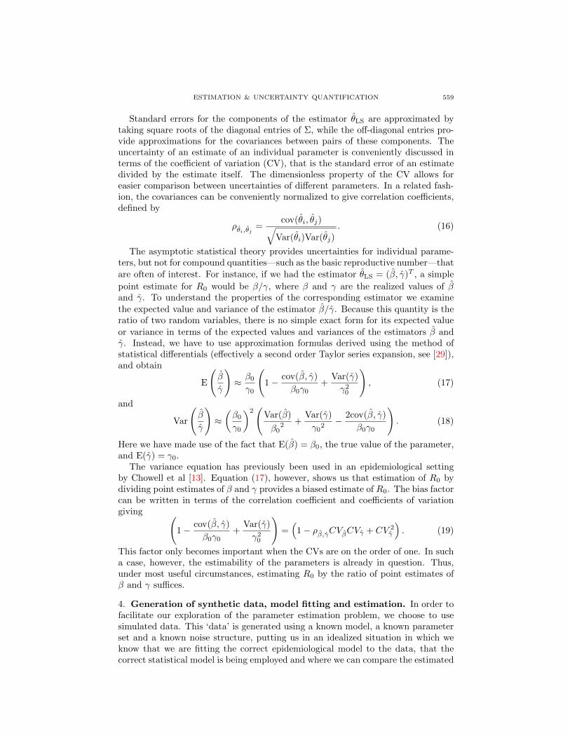
Standard errors for the components of the estimator θLS are approximated bytaking square roots of the diagonal entries of Σ, while the off-diagonal entries pro-vide approximations for the covariances between pairs of these components. Theuncertainty of an estimate of an individual parameter is conveniently discussed interms of the coefficient of variation (CV), that is the standard error of an estimatedivided by the estimate itself. The dimensionless property of the CV allows foreasier comparison between uncertainties of different parameters. In a related fash-ion, the covariances can be conveniently normalized to give correlation coefficients,defined by

ρθi,θj =cov(θi, θj)√

Var(θi)Var(θj). (16)

The asymptotic statistical theory provides uncertainties for individual parame-ters, but not for compound quantities—such as the basic reproductive number—that

are often of interest. For instance, if we had the estimator θLS = (β, γ)T , a simple

point estimate for R0 would be β/γ, where β and γ are the realized values of βand γ. To understand the properties of the corresponding estimator we examine

the expected value and variance of the estimator β/γ. Because this quantity is theratio of two random variables, there is no simple exact form for its expected value

or variance in terms of the expected values and variances of the estimators β andγ. Instead, we have to use approximation formulas derived using the method ofstatistical differentials (effectively a second order Taylor series expansion, see [29]),and obtain

E

(β

γ

)≈ β0γ0

(1− cov(β, γ)

β0γ0+

Var(γ)

γ20

), (17)

and

Var

(β

γ

)≈(β0γ0

)2(

Var(β)

β02 +

Var(γ)

γ02− 2cov(β, γ)

β0γ0

). (18)

Here we have made use of the fact that E(β) = β0, the true value of the parameter,and E(γ) = γ0.

The variance equation has previously been used in an epidemiological settingby Chowell et al [13]. Equation (17), however, shows us that estimation of R0 bydividing point estimates of β and γ provides a biased estimate of R0. The bias factorcan be written in terms of the correlation coefficient and coefficients of variationgiving (

1− cov(β, γ)

β0γ0+

Var(γ)

γ20

)=(

1− ρβ,γCVβCVγ + CV 2γ

). (19)

This factor only becomes important when the CVs are on the order of one. In sucha case, however, the estimability of the parameters is already in question. Thus,under most useful circumstances, estimating R0 by the ratio of point estimates ofβ and γ suffices.

4. Generation of synthetic data, model fitting and estimation. In order tofacilitate our exploration of the parameter estimation problem, we choose to usesimulated data. This ‘data’ is generated using a known model, a known parameterset and a known noise structure, putting us in an idealized situation in which weknow that we are fitting the correct epidemiological model to the data, that thecorrect statistical model is being employed and where we can compare the estimated

560 CAPALDI, BEHREND, BERMAN, SMITH, WRIGHT AND LLOYD

parameters with their true values. Furthermore, since we know the noise process,we can generate multiple realizations of the data set and hence directly assess theuncertainty in parameter estimates by fitting the model to each of the replicate datasets. As a consequence, we can more completely evaluate the performance of theestimation process than would be possible using a single real-world data set.

The use of synthetic data also allows us to investigate parameter estimation fordiseases that have differing levels of transmissibility. We considered three hypo-thetical infections, with low, medium and high transmissibility, using R0 values of1.2, 3 and 10, respectively. In each case we took the recovery rate γ to equal 1,which corresponds to measuring time in units of the average infectious period. Thevalue of β was then chosen to provide the desired value of R0. (In terms of the“true values” of our statistical model, we have γ0 = 1 and β0 = R0). We took apopulation size of 10, 000, of which 100 people were initially infectious, with theremainder being susceptible. (Altering the initial number of infectives makes noqualitative difference to the results that follow.)

The model was solved for S and I using the MATLAB ode45 routine, starting fromt = 0, giving output at n+ 1 evenly spaced time points (0, t1, ..., tn). The durationof the outbreak depends on R0 and so, in order to properly capture the time scaleof the epidemic, we choose tn to be the time at which I(t) falls back to its initialvalue. A data set for prevalence was then obtained by adding noise generated bymultiplying independent draws, ei, from a normal distribution with mean zero andvariance σ2

0 by I(ti, θ0)ξ. Thus, our data,

y(ti, θ0) ≡ I(ti, θ0) + I(ti, θ0)ξei, i = 1, 2, . . . , n, (20)

satisfies the assumptions made in Section 3 and allows us to apply the asymptoticstatistical theory. Notice that, for convenience, we have chosen normally distributedei, but we re-emphasize that the asymptotic statistical theory does not require this.Data sets depicting incidence of infection can be created in a similar way, replacingI(ti) by S(ti)− S(ti−1), as discussed above, for i = 1, . . . , n.

Three different values of ξ, namely ξ = 0 (absolute noise), ξ = 1/2 (Poissonnoise) and ξ = 1 (relative noise), were used to generate synthetic data sets. Giventhat prevalence (or incidence) increases with R0, the use of absolute noise, with thesame value of σ2

0 across the three transmissibility scenarios, leads to noise beingmuch more noticeable for the low transmissibility situation. This complicates com-parisons of the success of the estimation process between differing R0 values. Visualinspection of real-world data sets, however, indicates that variability increases witheither prevalence or incidence [23]. If this variability reflected reporting errors, withindividual cases being reported independently with some fixed probability, the vari-ance of the resulting binomial random variable would be proportional to its meanvalue. As a result, we direct most of our attention to data generated using ξ = 1/2.

Because we know the true values of the parameters and the variance of the noise,we can calculate the variance-covariance matrix Σ0 (Equation 8) exactly, withouthaving to use estimated parameter values or error variance. This provides a morereliable value than that obtained using the estimate Σ, allowing us to more easilydetect small changes in standard errors, such as those that occur when a single datapoint is removed from or added to a data set as we do in Section 6. This approachwas employed to obtain many of the results that follow (in each instance, it will bestated whether Σ0 or Σ was used to provide uncertainty estimates).

ESTIMATION & UNCERTAINTY QUANTIFICATION 561

5. Results: Parameter estimation. We could attempt to fit any combinationof the parameters and initial conditions of the SIR model, i.e., β, γ, N , S0 andI0. We shall concentrate, however, on the simpler situation in which we just fit βand γ, imagining that the other values are known. This might be the case if a newpathogen were introduced into a population at a known time, so that the populationwas known to be entirely susceptible apart from the initial infective. Importantly,the estimation of β and γ allows us to estimate the value of R0. We shall return toconsider estimation of three or more parameters in a later section.

The least squares estimation procedure works well for synthetic data sets gen-erated using the three different values of R0 (results not shown). Diagnostic plotsof the residuals were used to examine potential departures from the assumptionsof the statistical model: unsurprisingly, none were seen when the value of ξ usedin the fitting process matched that used to generate the data, and clear deviationswere seen when the incorrect value of ξ was used in the fitting process (results notshown).

Table 1. Coefficients of variation (CV) for parameter estimates ofβ, γ, R0, and the correlation coefficient between β and γ, ρβ,γ . Thecoefficients of variation and correlation coefficient were obtainedfrom the asymptotic stastical theory where the variance-covariancematrix Σ0 was calculated exactly (i.e., no curve-fitting was carriedout). Calculations were done under a Poisson noise structure, ξ =1/2, with σ2

0 = 1, and n = 50 data points. Parameter values andinitial conditions used were β = R0, γ = 1, N = 10, 000, S0 = 9900,and I0 = 100.

Parameter Value CVβ 1.2 0.0121γ 1 0.0110R0 1.2 0.0023ρβ,γ 0.9837 -

Parameter Value CVβ 3 0.0019γ 1 0.0034R0 3 0.0037ρβ,γ 0.1132 -

Parameter Value CVβ 10 0.0035γ 1 0.0027R0 10 0.0050ρβ,γ -0.3122 -

A Monte Carlo approach can be used to verify the distributional results of theasymptotic statistical theory. A set of point estimates of the parameter (β, γ) wasgenerated by applying the estimation process to a large number of replicate datasets generated using different realizations of the noise process, allowing estimates ofvariances and covariances of parameter estimates to be directly obtained. Unsur-prisingly, good agreement was seen when the correct value of ξ was employed in theestimation process and the distribution of (β, γ) estimates appears to be consistentwith the appropriate bivariate normal distribution predicted by the theory.

Table 1 and Figure 1a demonstrate that estimates of β and γ are correlated,with the sign and magnitude of the correlation coefficient depending strongly onthe value of R0. Standard errors for the estimates also depend strongly on thevalue of R0 (Figure 1b).

562 CAPALDI, BEHREND, BERMAN, SMITH, WRIGHT AND LLOYD

0 5 10 15R

0

-0.4

-0.2

0

0.2

0.4

0.6

0.8

1ρ

0 5 10 15R

0

0.001

0.01

0.1

1

10

100

1000

σ β or

σγ

a) b)

Figure 1. Dependence of the correlation coefficient and standarderrors for estimates of β and γ on the value of R0. Panel (a) displaysthe correlation coefficient, ρ, between estimates of β and γ for arange of R0 values. Panel (b) shows, on a log scale, standard errorsfor estimates of β (solid curve) and γ (dashed curve). The variance-covariance matrix Σ0 was calculated exactly (i.e., no curve-fittingwas carried out) under a Poisson noise structure, ξ = 1/2, withσ20 = 1, and n = 250 data points. Parameter values and initial

conditions used were β = R0, γ = 1, N = 10, 000, S0 = 9900, andI0 = 100.

As R0 approaches 1, the correlation coefficient approaches 1 and the standarderrors become extremely large. It is, therefore, difficult to obtain good estimates ofthe individual parameters in this case. Examination of the cost functional J in the(γ, β) plane reveals the origin of the strong correlation and large standard errors(Figure 2a). Near its minimum value, the contours of J are well approximated bylong thin ellipses whose major axes are oriented along the line β = R0γ. Thus thereis a considerable range of β and γ values that give almost identical model fits, butfor which the ratio β/γ varies relatively little. In a later section we shall see thatthese long thin elliptical contours arise as a consequence of sensitivities of the modelto changes in β and γ being almost equal in magnitude but of opposite signs. (Thederivation of these contour curves can be found in [9].)

For values of R0 that lead to lower correlation between estimates of β and γ,the contours of J near its minimum point are closer to being circular and are lesstilted (Figure 2b), allowing for easier identification of the two individual parameters.The standard error for the estimate of γ is seen to decrease with R0, while that ofβ exhibits non-monotonic behavior. For a fixed value of γ, increasing R0 leads tomore rapid spread of the infection and hence an earlier and higher peak in prevalence(Figure 3). For large values of R0, the majority of the transmission events occurover the timespan of the first few data points, meaning that fewer points withinthe data set are informative regarding the spread of the infection. Consequently, itbecomes increasingly difficult to estimate β as R0 is increased beyond some criticalvalue.

ESTIMATION & UNCERTAINTY QUANTIFICATION 563

0.80 0.90 1.00 1.10 1.20γ

1.00

1.10

1.20

1.30

1.40

β

0.80 0.90 1.00 1.10 1.20γ

2.80

2.90

3.00

3.10

3.20

β

0.80 0.90 1.00 1.10 1.20γ

9.80

9.90

10.00

10.10

10.20

β

1000

1000

0050

000

1000

0

5000

0

1000

0010

000

(a)

(b)

1000

1000

00

5000

0

1000

0

5000

0

1000

00

(c)

1000

1000

0

1000

0

5000

0

1000

00

5000

0

1000

00

Figure 2. Contours of the cost functional J in the (γ,β)-plane(solid curves) for R0 equal to (a) 1.2, (b) 3, and (c) 10. A Poissonnoise structure was assumed (ξ = 1/2), with σ2

0 = 1 and n = 50data points. Parameter values and initial conditions used wereβ = R0, γ = 1, N = 10, 000, S0 = 9900, and I0 = 100. Contoursare at heights 1000, 2500, 5000, 7500, 10000, 25000, 50000, 75000and 100000. For clarity, not all contours are labeled with theirheight.

As seen in Table 1, estimates of β and γ have relatively large uncertainties whenR0 is small. It would, for instance, be difficult to accurately estimate the averageduration of infection, 1/γ, for an infection such as seasonal influenza—which istypically found to have R0 about 1.3 (ranging from 0.9 to 2.1) [14]—using the leastsquares approach. Importantly, however, the estimate of R0 has a much lowervariation (as measured by the CV) than the estimates of β and γ. The strongpositive correlation between the estimates of β and γ reduces the variance of theR0 estimate, as can be seen in Equation (18), and reflecting the earlier observationconcerning the orientation of the contours of the cost functional along lines of theform β = R0γ.

6. Results: Sampling schemes and uncertainty of estimates. Biologicaldata is often difficult or costly to collect, so it is desirable to collect data in such away to maximize its informativeness. Consequently it is important to understandhow parameter estimation depends on the number of sampled data points and thetimes at which the data are collected. This information can then be used to guide

564 CAPALDI, BEHREND, BERMAN, SMITH, WRIGHT AND LLOYD

future data collection. In this section we examine two approaches to address thisquestion: sensitivity analysis and data sampling.

6.1. Sensitivity. The sensitivities of a system provide temporal information onhow states of the system respond to changes in the parameters [21, 37]. They can,therefore, be used to identify time intervals where the system is most sensitive tosuch changes. Noting that the sensitivities are used to calculate the standard errorsin estimates of parameters, direct observation of the sensitivity function providesan indication of time intervals in which data points carry more or less informationfor the estimation process [4, 5]. For instance, if the sensitivity to some parameteris close to zero in some time interval, changes in the value of the parameter wouldhave little impact on the state variable. Conversely, more accurate knowledge ofthe state variable at that time could not cause the estimated parameter value tochange by much.

For low values of R0, for example R0 = 1.2, we see that the sensitivity func-tions of I(t) with respect to β and γ are near mirror images of each other (Figure3a). This mirror image phenomenon allows a change in one parameter to be easilycompensated by a corresponding change in the other parameter, giving rise to thestrong correlation between the estimates of the two parameters. Early in the epi-demic, we see a similar phenomenon for all values of R0. We comment further onthis observation in the next section.

As R0 increases, the two sensitivity functions take on quite different shapes.Prevalence is much less sensitive to changes in β than to changes in γ. The sensi-tivity of prevalence to β is greatest right before the epidemic peak, before becomingnegative, but small, during the late stages of the outbreak. The sensitivity becomesnegative because an increase in β would cause the peak of the outbreak to occurearlier, reducing the prevalence at a fixed, later time. I remains sensitive withrespect to γ throughout much of the epidemic, reaching its largest absolute valueslightly later than the time at which the outbreak peaks.

While the sensitivity functions provide an indication of when additional, or moreaccurate data, is likely to be informative, they have clear limitations, not leastbecause they do not provide a quantitative measure of how uncertainty estimates,such as standard errors, are impacted. Being a univariate approach they cannotaccount for any impact of correlation between parameter estimates, as we shallsee below, although they can indicate instances in which parameter estimates arelikely to be correlated. Furthermore, they do not account for the different weightingaccorded to different data points on account of the error structure of the model,such as the relationship between error variance and the magnitude of the observa-tion being made. Another type of sensitivity function, the generalized sensitivityfunction (GSF) introduced by Thomaseth and Cobelli [40], which is based on theFisher information matrix, does account for these two factors. While the GSF doesprovide qualitative information that can guide data collection, its interpretation isnot without its own complications [4] and, given that we found that it providedlittle additional insight in the current setting, we shall not discuss it further here.

6.2. Data sampling. In order to gain quantitative information about samplingschemes on parameter estimation, as opposed to the qualitative information pro-vided by inspection of the sensitivity functions, we carried out three numericalexperiments in which different sampling schemes were implemented. The first ap-proach involves altering the frequency at which data are sampled within a fixed

ESTIMATION & UNCERTAINTY QUANTIFICATION 565

-1500

-1000

-500

0

500

1000

1500Se

nsiti

vity

-4000

-3000

-2000

-1000

0

1000

2000

3000

Sens

itivi

ty-4000

-3000

-2000

-1000

0

1000

2000

Sens

itivi

ty

0 5 10 15t

50

100

150

200

250

Prev

alen

ce

0 2 4 6 8t

0

1000

2000

3000

Prev

alen

ce

0 2 4 6t

0

2000

4000

6000

Prev

alen

ce

(a) (b) (c)

Figure 3. Sensitivities of I(t) (i.e., prevalence) with respect to themodel parameters β (solid curves) and γ (dashed curves) are shownon the upper panels of the graphs for a) R0 = 1.2, b) R0 = 3 and c)R0 = 10. The lower panel of each graph displays the correspondingprevalence-time curve. The initial conditions of the SIR model wereS0 = 9900, I0 = 100, with N = 10, 000 and γ was taken equal toone, so β = R0.

observation window that covers the duration of the outbreak. The second approachconsiders sampling at a fixed frequency but over observation windows of differingdurations. The third approach examines increasing the sampling frequency withinspecified sub-intervals of a fixed observation window.

In the first sampling method we alter the frequency at which observations aretaken while keeping the observation window fixed. In other words, we increase nwhile fixing t0 = 0 and tn = tend. For incidence data, increasing the observationfrequency—i.e., reducing the period over which each observation is made—has theimportant effect of reducing the values of the observed data and the correspondingmodel values. Under relative observational error (ξ = 1) there is a correspondingchange in the error variance, keeping a constant signal to noise ratio. If ξ < 1,increasing n decreases the signal to noise ratio of the data.

Adding additional data points in this way increases the accuracy of parameterestimates, with standard errors eventually decreasing as n−1/2 (Figure 4, in whichprevalence data is used), in accordance with the asymptotic theory [39]. This isstill the case for incidence data even when ξ < 1 where the signal to noise ratiodecreases in n. We point out that changing the sampling frequency will typicallynot be an option in epidemiological settings because data will be collected at somefixed frequency, such as once each day or week, although, conceivably, a weeklysampling frequency could be replaced by daily sampling.

566 CAPALDI, BEHREND, BERMAN, SMITH, WRIGHT AND LLOYD

10 100 1000n

0.001

0.01

0.1

1St

anda

rd e

rror

σ βor

σγ

Figure 4. Standard errors of β (solid curve) and γ (dashed curve)as the number of observations, n, changes while maintaining a con-stant window of observation (fixed tend). Apart from the smallestfew values of n, the points fall on a line of slope − 1

2 on this log-logplot. Standard errors are calculated using Equation (8), using thetrue values of the parameters. The variance-covariance matrix Σ0

was calculated exactly (i.e., no curve-fitting was carried out) withthe disease prevalence under a Poisson noise structure, ξ = 1/2,with σ2

0 = 1. Parameter values and initial conditions used wereβ = 3, γ = 1, N = 10, 000, S0 = 9900, and I0 = 100.

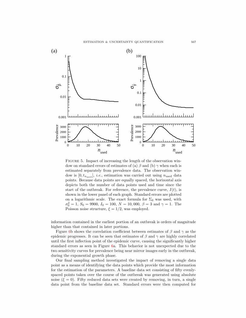
For real-time outbreak analysis, the amount of available data will increase overtime as the epidemic unfolds. Consequently, it is of practical importance to un-derstand how much data—and hence observation time—is required to obtain reli-able estimates and the extent to which estimates will improve with additional datapoints. Using Equation (8) and the known values of the parameters, we calculatedstandard errors for parameter estimates based on the first nused data points, wherep + 1 ≤ nused ≤ n. As seen in Figures 5a and 5b, when only one parameter is fit-ted, the standard error decreases rapidly at first, but its decrease slows significantlyjust before the peak of the epidemic. Once this point in time has been reached,subsequent data points provide considerably less additional information than didearlier data points. In this setting, the most important time interval extends fromthe initial infection to just before the peak of the outbreak. However, when bothβ and γ are fitted, the interval of steep descent extends slightly beyond the peakof the epidemic, as seen in Figure 6a. This indicates that it would be useful tocollect data over a longer interval in this case. Notice the log scale on the verticalaxis for each of the aforementioned plots. These figures suggest that the amount of

ESTIMATION & UNCERTAINTY QUANTIFICATION 567

0.001

0.01

0.1

1σ β^

0.001

0.01

0.1

1

10

100

σ γ

0 10 20 30 40 50

nused

0

1000

2000

3000

Prev

alen

ce

0 10 20 30 40 50

nused

0

1000

2000

3000

Prev

alen

ce

(a) (b)

Figure 5. Impact of increasing the length of the observation win-dow on standard errors of estimates of (a) β and (b) γ when each isestimated separately from prevalence data. The observation win-dow is [0, tnused

], i.e., estimation was carried out using nused datapoints. Because data points are equally spaced, the horizontal axisdepicts both the number of data points used and time since thestart of the outbreak. For reference, the prevalence curve, I(t), isshown in the lower panel of each graph. Standard errors are plottedon a logarithmic scale. The exact formula for Σ0 was used, withσ20 = 1, S0 = 9900, I0 = 100, N = 10, 000, β = 3 and γ = 1. The

Poisson noise structure, ξ = 1/2, was employed.

information contained in the earliest portion of an outbreak is orders of magnitudehigher than that contained in later portions.

Figure 6b shows the correlation coefficient between estimates of β and γ as theepidemic progresses. It can be seen that estimates of β and γ are highly correlateduntil the first inflection point of the epidemic curve, causing the significantly higherstandard errors as seen in Figure 6a. This behavior is not unexpected due to thetwo sensitivity curves for prevalence being near mirror images early in the outbreak,during the exponential growth phase.

Our final sampling method investigated the impact of removing a single datapoint as a means of identifying the data points which provide the most informationfor the estimation of the parameters. A baseline data set consisting of fifty evenly-spaced points taken over the course of the outbreak was generated using absolutenoise (ξ = 0). Fifty reduced data sets were created by removing, in turn, a singledata point from the baseline data set. Standard errors were then computed for

568 CAPALDI, BEHREND, BERMAN, SMITH, WRIGHT AND LLOYD

0.001

0.01

0.1

1

10

100σ β^

or

σγ

0

0.2

0.4

0.6

0.8

1

ρ

0 10 20 30 40 50

nused

0

1000

2000

3000

Prev

alen

ce

0 10 20 30 40 50

nused

0

1000

2000

3000Pr

eval

ence

(a) (b)

Figure 6. Illustrated in graph (a) is the impact of increasing thelength of the observation window on standard errors of estimatesof β (solid curve) and γ (dashed curve) when both are estimatedsimultaneously. Graph (b) displays the effect on the correlationcoefficient between estimates of β and γ. The observation windowconsists of nused data points in the time interval [t0, tnused

]. Forreference, the prevalence curve, I(t), is shown on the lower panels.All parameter values and other details are as in the previous figure.

the reduced data sets using the true covariance matrix Σ0 (Equation (8)). (Forthis experiment, use of the true covariance matrix allowed us to accurately observethe small effects on standard errors that resulted from the removal of single datapoints. Errors introduced by solving the inverse problem would have obscured thepatterns we observed.) The largest standard error values in this group of data setscorrespond to the most informative data points since the removal of such pointsleads to the largest increase in uncertainty of the estimate.

As Figure 7 shows, when β is the only parameter fitted and ordinary least squaresestimation is used, the local maxima of the standard error curve occur at the sametimes as the local extrema of the sensitivity curve, and the local minima occurwhen the sensitivity is close to zero. In this case, the sensitivity function correctlyidentifies subintervals in which data are most or least informative about β.

The picture is not quite as straightforward when β and γ are estimated simul-taneously using ordinary least squares. Figure 8 shows that the local maxima ofthe standard error curves no longer line up directly with the local extrema of thesensitivity curves (this effect is more easily seen in Figure 8b). This is likely due

ESTIMATION & UNCERTAINTY QUANTIFICATION 569

0 2 4 6 8t

-1000

-500

0

500

1000

1500

2000

2500

∂I/ ∂

β

0.0146

0.0150

0.0154

0.0158σ β^

Figure 7. Standard errors for the estimation of β from prevalencedata using the single point removal method as discussed in the text(solid curve) with the baseline standard error (without removingany points) also plotted (horizontal dashed line). Standard errorswere calculated using Equation (8) and each is plotted at the timeti corresponding to the removed data point. For comparison, thesensitivity of I(t) with respect to β is also shown (dotted curve).Synthetic data was generated using the parameter values σ2

0 = 104,S0 = 9900, I0 = 100, N = 10, 000, β = 3 and γ = 1. The additivenoise structure, ξ = 0 was assumed.

to the correlation between the estimates of β and γ: the off-diagonal terms ofχT(θ)W (θ)χ(θ) involve products of sensitivities with respect to the two differentparameters. As a consequence, it is no longer sufficient to examine individual sen-sitivity curves, but, as we have seen, the selective reductive method described here,based on the asymptotic theory, can identify when additional data should ideallybe sampled.

Similarly, having a weight matrix other than the identity (i.e., when GLS, ratherthan OLS, is to be used) leads to the sensitivity curves misidentifying the subinter-vals in which data are most or least informative for parameter estimation (resultsnot shown; see [9]). This occurs whether single or multiple parameters are esti-mated, and happens because the sensitivity curves do not, by themselves, accountfor the relative importance placed on different data points. Again, the selective re-duction method accounts for this effect and correctly identifies time intervals whenadditional data would be most informative.

7. Results: Parameter identifiability. Until now, we have only considered theintroduction of an infection into a virgin population, assuming a known initial num-ber of infectives in an otherwise susceptible population. For an endemic infection,such as seasonal flu, only a fraction of the population would be susceptible at thestart of an outbreak. In such instances, the general reproductive number, Rt, theaverage number of secondary infections at any point in time, is a more relevant

570 CAPALDI, BEHREND, BERMAN, SMITH, WRIGHT AND LLOYD

0 2 4 6 8t

-4500

-3000

-1000

0

∂I/ ∂

γ

0.0084

0.0086

0.0088

σ γ

0 2 4 6 8t

-1000

0

1000

2000

∂I/ ∂

β

0.0162

0.0165

0.0168

0.0171σ β^

(a) (b)

Figure 8. Standard errors for the simultaneous estimation of βand γ from prevalence data using the single point removal methodas discussed in the text (solid curves). Standard errors were cal-culated using Equation (8), and each is plotted at the time ti ofthe removed data point. Panel (a) shows the standard error for theestimate of β (solid curve), together with the baseline (i.e., with-out removing any points) standard error (horizontal dashed line)and the sensitivity of I(t) with respect to β (dotted curve). Panel(b) shows the standard error for the estimate of γ (solid curve),together with the baseline standard error (horizontal dashed line)and the sensitivity of I(t) with respect to γ (dotted curve). Allparameter values and other details are as in the previous figure.

quantity than R0. For the SIR model, Rt is given by

Rt = R0S(t)

N. (21)

In the virgin population considered above, we saw that as R0 approached one therewas considerable difficulty in independently estimating a pair of parameters. In theendemic setting, this phenomenon occurs as Rt approaches one, so the parameteridentifiability issue can arise even if R0 is significantly greater than one.

In the endemic setting, we would be unlikely to know the initial numbers ofinfectives and susceptibles, so we would also need to estimate the values of S0

and I0. Given the difficulty in estimating a pair of parameters that has alreadybeen illustrated, it seems reasonable to expect that parameter identfiability wouldbecome a more delicate issue if larger sets of parameters were estimated. In thissection we shall explore the identifiability of parameters when combinations of β,γ, S0 and I0 are estimated. This method is generally referred to as subset selectionand has been explored by in the context of identifiability by a number of authors(for example, [7, 8, 15, 28]).

It has been shown by Evans et al. in [22] that the SIR model with demographyis identifiable for all model parameters and initial conditions. They use a strictdefinition of non-identifiability, where in such a model, a change in one parametercan be compensated by changes in other parameters. However, the authors alsoconcede that while the model may be identifiable, that property alone does not giveinsight into the ease of estimation of certain subsets of parameters. For example,

ESTIMATION & UNCERTAINTY QUANTIFICATION 571

by their definition, two parameters whose estimates have a correlation coefficient of0.99 would be identifiable, yet they may not be easily estimated. In this section, weuse quantitative methods to assess ease of parameter identifiability in the contextof subset selection.

It was stated above that the asymptotic statistical theory requires the limitingmatrix Ω0 to be invertible. With a finite-sized sample, we instead require this of

Ω(n)0 . Non-identifiability leads to these matrices being singular, or close to singular

[8], and so one method for determining whether model parameters are identifiable

involves calculating the condition number of Ω(n)0 , or, equivalently the condition

number of the matrix Σ(n) [15]. The condition number, κ(X), of a nonsingularmatrix X is defined to be the product of the norm of X and the norm of X−1.If we take the norm to be the usual induced matrix 2-norm, we have that thecondition number of X is the ratio of the largest singular value (from a singularvalue decomposition) of X to the smallest singular value of X [34].

Initially, we investigate the case where only β and γ are fitted. In this situation,we are able to find an expression for κ(Σ)

κ(Σ) =σ2β

+ σ2γ +

√σ4β

+ σ4γ − 2σ2

βσ2γ + 4ρ2

β,γσ2βσ2γ

σ2β

+ σ2γ −

√σ4β

+ σ4γ − 2σ2

βσ2γ + 4ρ2

β,γσ2βσ2γ

. (22)

If the standard errors were fixed, Equation 22 shows that as the correlation be-tween estimates of β and γ approaches one, the condition number goes to infinity.However, in reality standard errors do depend on the values of β and γ; Figure9 provides a more complete picture of how the condition number changes over arange of R0 values. As the figure shows, it is more difficult to rely on estimates ofβ and γ when R0 approaches one, corroborating what we have previously seen forthe correlation coefficient (see Figure 1a).

Numerical experiments indicate that when more parameters are fitted to thedata, identifiability becomes a more serious issue. In such a case, while we can nolonger give a simple expression for κ(Σ0) since it is a function of the parameters, theinitial conditions and even the data, it provides insight into parameter identifiability.We examine κ(Σ0) across different subsets of fitted parameters as seen in Table 2.As we increase the number of parameters fitted, the condition number can increaseby multiple orders of magnitude. This is evident whenever we fit both β and S0.Notice that for the larger κ values, the magnitude of ρ is very near to one, indicatingstrong correlation. Thus, we can surmise that as we increase the number of fittedparameters, our ability to identify individual parameters decreases, especially if theparameters added to θ have correlated estimates.

In this example, if we assume the initial conditions are known, our ability toestimate β and γ is good. Yet, once we have to estimate one or both initial coni-ditions, our ability to estimate either β or γ worsens considerably. Given that inmost situations initial conditions are not known exactly, parameter identifiabilityhas the potential to be of widespread concern.

8. Discussion. Parameter values estimated from real-world data will always beaccompanied by some uncertainty. Estimates of this uncertainty allow us to judgehow reliable the parameter estimates are and how much faith should be put inany predictions made on their basis. As such, uncertainty estimates should always

572 CAPALDI, BEHREND, BERMAN, SMITH, WRIGHT AND LLOYD

0 5 10 15R

0

100

102

104

106

108

1010

κ (Σ

0)

Figure 9. Dependence of the condition number of the 2 × 2variance-covariance matrix (fitting β and γ) on the value of R0.The condition number is displayed on a log scale. The variance-covariance matrix Σ0 was calculated exactly (i.e., no curve-fittingwas carried out) under a Poisson noise structure, ξ = 1/2, withσ20 = 1, and n = 250 data points. Parameter values and initial

conditions used were β = R0, γ = 1, N = 10, 000, S0 = 9900, andI0 = 100.

Table 2. Standard errors of β and γ, the correlation coefficientbetween estimates of β and γ and the condition number of theχTWχ matrix when R0 = 3 when fitting different sets of parame-ters. ξ = 1/2, N = 10, 000, S0 = 9900, I0 = 100, β = R0, γ = 1and σ2

0 = 104.

Parameters Fitted σβ σγ ρ κ

β, γ 0.3419 0.1142 -0.2067 5.2211× 100

β, γ, S(0) 17.094 1.9936 -0.9984 5.5760× 109

β, γ, I(0) 1.7536 0.1176 0.3534 1.2000× 106

β, γ, S(0), I(0) 44.655 3.3060 -0.9548 1.4383× 1010

accompany estimates of parameter values. The asymptotic statistical theory em-ployed here provides a reasonably straightforward way to obtain such informationwhen least-squares fitting is used as the estimation process.

The use of a number of synthetic data sets, generated under a number of differentscenarios concerning the transmissibility of infection, has allowed us to get a broader

ESTIMATION & UNCERTAINTY QUANTIFICATION 573

understanding of the parameter estimation process than would have been possible ifwe had limited attention to a single data set. As we have demonstrated, the uncer-tainties that accompany parameter estimation, and even our ability to separatelyidentify parameters—even with this simplest of SIR models—can be extremely var-ied based on the underlying parameter values and the parameter set being fitted.A primary reason for difficulties in estimation and identifiability stems from corre-lations between parameter estimates. Even if individual parameter estimates havelarge uncertainties it can still be possible to estimate epidemiologically importantinformation, e.g., the basic reproductive number R0, with much less uncertainty.

Increasing the number of observations made at critical times during the epidemiccan provide a substantial gain in the precision of the estimation process. While thesensitivity equations of the model provide a general idea of times at which additionaldata will be most informative, they do not tell the whole story. The asymptoticstatistical theory, together with the data point removal technique, can be used toguide data collection. This approach can be employed once a parameter set isknown: this might be one based on a preliminary set of estimates, expert opinon,or even a best-guess. Some aspects of our discussion do, however, require moredetailed information on the magnitude and nature of the noise in the data.

We have focused on identifiability in the least squares context, but one cannotescape a lack of parameter identifiability simply by using a different method ofparameter estimation. Bayesian methods, including Markov Chain Monte Carlo,(see, for example, [11] and [31]), provide an alternative suite of approaches that arecommonly used to solve the inverse problem. Yet, since identifiability is primarilya feature of the mathematical model and less dependent on the fitting process,switching estimation techniques often does not remove the problem of parameteridentifiability, so it remains an important concern when solving the inverse problemin any respect.

It should be noted that all experiments presented here were conducted withknowledge of the underlying model, that is, the correct model was fit to the data.However, in scenarios with real data this assumption is not valid and results in afurther layer of uncertainty. This type of structural uncertainty has received far lessattention but in some circumstances it can dwarf uncertainty due to noise in thedata. As an example, a number of authors have shown that estimates of the basicreproductive number obtained by fitting models to data on the initial growth of anoutbreak can be highly sensitive to model assumptions [32, 33, 35, 42].

We chose to focus our attention on perhaps the simplest possible setting forthe estimation process, one for which the SIR model was appropriate. Unfortu-nately, few real-world disease transmission processes are quite this simple; in mostinstances, a more complex epidemiological model, accompanied by a larger set ofparameters and initial conditions, would be more realistic. It is not hard to imag-ine that many of the issues discussed here would be much more delicate in suchsituations: parameter identifiability, in particular, could be a major concern. Theapproach employed here would reveal whether such problems would accompany es-timation using a given model, and indeed can be used to guide the selection ofmodels and/or parameter sets that can be used or estimated reliably. Again, thisemphasizes the need for the estimation process to be accompanied by some accountof the uncertainties, but not only in terms of uncertainties of individual estimatesbut also of correlation between estimates.

574 CAPALDI, BEHREND, BERMAN, SMITH, WRIGHT AND LLOYD

Acknowledgments. We would like to thank the referees for their valuable com-ments and suggestions. This work was funded by Research Experiences for Un-dergraduates grants from the National Science Foundation (DMS-0552571) and theNational Security Agency (H98230-06-1-0098), and by the Center for QuantitativeSciences in Biomedicine, North Carolina State University. Funding support alsocame from the Research and Policy for Infectious Disease Dynamics (RAPIDD)program of the Science and Technology Directory, Department of Homeland Secu-rity, and Fogarty International Center, National Institutes of Health. Preliminaryresults of Sections 5 (Parameter Estimation) and 6.1 (Sensitivity) originated froma summer REU project. These sections, and the remainder of the work, were thendeveloped by the first author.

Appendix: Sensitivity equations for the SIR model. Here we present thesensitivity equations that are relevant for SIR model-based estimation. If preva-lence data is being used, then the relevant sensitivities are ∂I(ti)/∂θ. Analysis ofincidence data would instead make use of ∂S(ti−1)/∂θ−∂S(ti)/∂θ. (Recall that, forthe SIR model considered here, the number of cases that occur over a time intervalis equal to the decrease in the number of susceptibles over that time).

Writing the sensitivities of the state variables with respect to the model param-eters as φ1 = ∂S/∂β, φ2 = ∂S/∂γ, φ3 = ∂I/∂β, and φ4 = ∂I/∂γ, the followingsensitivity equations are obtained

dφ1dt

= −βINφ1 −

βS

Nφ3 −

SI

N(23)

dφ2dt

= −βINφ2 −

βS

Nφ4 (24)

dφ3dt

=βI

Nφ1 +

(βS

N− γ)φ3 +

SI

N(25)

dφ4dt

=βI

Nφ2 +

(βS

N− γ)φ4 − I, (26)

with the initial conditions φ1(0) = φ2(0) = φ3(0) = φ4(0) = 0.For the sensitivities of the state variables with respect to initial conditions, writ-

ing φ5 = ∂S/∂S0, φ6 = ∂S/∂I0, φ7 = ∂I/∂S0, and φ8 = ∂I/∂I0, we have that

dφ5dt

= −βINφ5 −

βS

Nφ7 (27)

dφ6dt

= −βINφ6 −

βS

Nφ8 (28)

dφ7dt

=βI

Nφ5 +

(βS

N− γ)φ7 (29)

dφ8dt

=βI

Nφ6 +

(βS

N− γ)φ8, (30)

together with the initial conditions φ5(0) = φ8(0) = 1, and φ6(0) = φ7(0) = 0.

REFERENCES

[1] R. M. Anderson and R. M. May, “Infectious Diseases of Humans,” Oxford University Press,

Oxford, 1991.[2] D. T. Anh, M. P. Bonnet, G. Vachaud, C. V. Minh, N. Prieur, L. V. Duc and L. L. Anh,

Biochemical modeling of the Nhue River (Hanoi, Vietnam): Practical identifiability analysis

and parameters estimation, Ecol. Model., 193 (2006), 182–204.

ESTIMATION & UNCERTAINTY QUANTIFICATION 575

[3] H. T. Banks, M. Davidian, J. R. Samuels Jr. and K. L. Sutton, An inverse problem statisti-cal methodology summary, in “Mathematical and Statistical Estimation Approaches in Epi-

demiology” (eds. G. Chowell, J. M. Hyman, L. M. A. Bettencourt and C. Castillo-Chavez),

Springer, New York, (2009), 249–302.[4] H. T. Banks, S. Dediu and S. L. Ernstberger, Sensitivity functions and their uses in inverse

problems, Tech. Report CRSC-TR07-12, Center for Research in Scientific Computation, NorthCarolina State Unversity, July 2007.

[5] H. T. Banks, S. L. Ernstberger and S. L. Grove, Standard errors and confidence intervals in

inverse problems: Sensitivity and associated pitfalls, J. Inverse Ill-Posed Probl., 15 (2007),1–18.

[6] R. Bellman and K. J. Astrom, On structural identifiability, Math. Biosci., 7 (1970), 329–339.

[7] R. Brun, M. Kuhni, H. Siegrist, W. Gujer and P. Reichert, Practical identifiability of ASM2dparameters–systematic selection and tuning of parameter subsets, Water Res., 36 (2002),

4113–4127.

[8] M. Burth, G. C. Verghese and M. Velez-Reyes, Subset selection for improved parameterestimation in on-line identification of a synchronous generator , IEEE Trans. Power Syst.,

14 (1999), 218–225.

[9] A. Capaldi, S. Behrend, B. Berman, J. Smith, J. Wright and A. L. Lloyd, Parameter esti-mation and uncertainty quantification for an epidemic model, Tech. Report CRSC-TR09-18,

Center for Research in Scientific Computation, North Carolina State Unversity, August 2009.[10] S. Cauchemez, P.-Y. Boelle, G. Thomas and A.-J. Valleron, Estimating in real time the

efficacy of measures to control emerging communicable diseases, Am. J. Epidemiol., 164

(2006), 591–597.[11] S. Cauchemez and N. M. Ferguson, Likelihood-based estimation of continuous-time epidemic

models from time-series data: Application to measles transmission in London, J. R. Soc.

Interface, 5 (2008), 885–897.[12] G. Chowell, C. E. Ammon, N. W. Hengartner and J. M. Hyman, Estimating the reproduction

number from the initial phase of the Spanish flu pandemic waves in Geneva, Switzerland ,

Math. Biosci. Eng., 4 (2007), 457–470.[13] G. Chowell, N. W. Hengartner, C. Castillo-Chavez, P. W. Fenimore and J. M. Hyman, The

basic reproductive number of ebola and the effects of public health measures: The cases of

Congo and Uganda, J. Theor. Biol., 229 (2004), 119–126.[14] G. Chowell, M. A. Miller and C. Viboud, Seasonal influenza in the United States, France and

Australia: Transmission and prospects for control, Epidemiol. Infect., 136 (2007), 852–864.[15] A. Cintron-Arias, H. T. Banks, A. Capaldi and A. L. Lloyd, A sensitivity matrix based

methodology for inverse problem formulation, J. Inv. Ill-Posed Problems, 17 (2009), 545–564.

[16] A. Cintron-Arias, C. Castillo-Chavez, L. M. A. Bettencourt, A. L. Lloyd and H. T. Banks,The estimation of the effective reproductive number from disease outbreak data, Math. Biosci.

Eng., 6 (2009), 261–282.[17] C. Cobelli and J. J. DiStefano, III, Parameter and structural identifiability concepts and

ambiguities: A critical review and analysis, Am. J. Physiol. (Regulatory Integrative Comp.

Physiol. 8), 239 (1980), R7–R24.

[18] M. Davidian and D. M. Giltinan, “Nonlinear Models for Repeated Measurement Data,” Chap-man & Hall, 1996.

[19] O. Diekmann and J. A. P. Heesterbeek, “Mathematical Epidemiology of Infectious Diseases.Model Building, Analysis and Interpretation,” Wiley Series in Mathematical and Computa-tional Biology, John Wiley & Sons, Ltd., Chichester, 2000.

[20] K. Dietz, The estimation of the basic reproduction number for infectious diseases, Stat. Meth.

Med. Res., 2 (1993), 23–41.[21] M. Eslami, “Theory of Sensitivity in Dynamic Systems. An Introduction,” Springer-Verlag,

Berlin, 1994.[22] N. D. Evans, L. J. White, M. J. Chapman, K. R. Godfrey and M. J. Chappell, The structural

identifiability of the susceptible infected recovered model with seasonal forcing, Math. Biosci.,

194 (2005), 175–197.[23] B. Finkenstadt and B. Grenfell, Empirical determinants of measles metapopulation dynamics

in England and Wales, Proc. R. Soc. Lond. B, 265 (1998), 211–220.

[24] K. Glover and J. C. Willems, Parametrizations of linear dynamical systems: Canonical formsand identifiability, IEEE Trans. Auto. Contr., AC-19 (1974), 640–646.

[25] H. W. Hethcote, The mathematics of infectious diseases, SIAM Rev., 42 (2000), 599–653.

576 CAPALDI, BEHREND, BERMAN, SMITH, WRIGHT AND LLOYD

[26] T. D. Hollingsworth, N. M. Ferguson and R. M. Anderson, Will travel restrictions control theinternational spread of pandemic influenza? , Nature Med., 12 (2006), 497–499.

[27] A. Holmberg, On the practical identifiability of microbial growth models incorporating

Michaelis-Menten type nonlinearities, Math. Biosci., 62 (1982), 23–43.[28] J. A. Jacquez and P. Greif, Numerical parameter identifiability and estimability: Integrating

identifiability, estimability and optimal sampling design, Math. Biosci., 77 (1985), 201–227.[29] S. Kotz, N. Balakrishnan, C. Read and B. Vidakovic, eds., “Encyclopedia of Statistics,” 2nd

edition, Wiley-Interscience, Hoboken, New Jersey, 2006.

[30] M. Kretzschmar, S. van den Hof, J. Wallinga and J. van Wijngaarden, Ring vaccination andsmallpox control , Emerg. Inf. Dis., 10 (2004), 832–841.

[31] P. E. Lekone and B. F. Finkenstadt, Statistical inference in a stochastic epidemic SEIR model

with control intervention: Ebola as a case study, Biometrics, 62 (2006), 1170–1177.[32] A. L. Lloyd, The dependence of viral parameter estimates on the assumed viral life cycle:

Limitations of studies of viral load data, Proc. R. Soc. Lond. B, 268 (2001), 847–854.

[33] , Sensitivity of model-based epidemiological parameter estimation to model assump-tions, in “Mathematical and Statistical Estimation Approaches in Epidemiology” (eds.

G. Chowell, J. M. Hyman, L. M. A. Bettencourt and C. Castillo-Chavez), Springer, NewYork, (2009), 123–141.

[34] C. D. Meyer, “Matrix Analysis and Applied Linear Algebra,” SIAM, Hoboken, New Jersey,

2000.[35] M. A. Nowak, A. L. Lloyd, G. M. Vasquez, T. A. Wiltrout, L. M. Wahl, N. Bischofberger,

J. Williams, A. Kinter, A. S. Fauci, V. M. Hirsch and J. D. Lifson, Viral dynamics of primary

viremia and antiretroviral therapy in simian immunodeficiency virus infection, J. Virol., 71(1997), 7518–7525.

[36] J. G. Reid, Structural identifiability in linear time-invariant systems, IEEE Trans. Auto.

Contr., AC-22 (1977), 242–246.[37] A. Saltelli, K. Chan and E. M. Scott, eds., “Sensitivity Analysis,” Wiley Series in Probability

and Statistics, John Wiley & Sons, Ltd., Chichester, 2000.

[38] M. A. Sanchez and S. M. Blower, Uncertainty and sensitivity analysis of the basic reproductiverate, Am. J. Epidemiol., 145 (1997), 1127–1137.

[39] G. A. F. Seber and C. J. Wild, “Nonlinear Regression,” John Wiley & Sons, Hoboken, NewJersey, 2003.

[40] K. Thomaseth and C. Cobelli, Generalized sensitivity functions in physiological system iden-

tification, Ann. Biomed. Eng., 27 (1999), 607–616.[41] J. Wallinga and M. Lipsitch, How generation intervals shape the relationship between growth

rates and reproductive numbers, Proc. R. Soc. Lond. B, 274 (2007), 599–604.

[42] H. J. Wearing, P. Rohani and M. Keeling, Appropriate models for the management of infec-tious diseases, PLoS Med., 2 (2005), e174.

[43] L. J. White, N. D. Evans, T. J. G. M. Lam, Y. H. Schukken, G. F. Medley, K. R. Godfreyand M. J. Chappell, The structural identifiability and parameter estimation of a multispeciesmodel for the transmission of mastitis in dairy cows, Math. Biosci., 174 (2001), 77–90.

[44] H. Wu, H. Zhu, H. Miao and A. S. Perelson, Parameter identifiability and estimation of

HIV/AIDS dynamic models, Bull. Math. Biol., 70 (2008), 785–799.[45] X. Xia and C. H. Moog, Identifiability of nonlinear systems with application to HIV/AIDS

models, IEEE Trans. Auto. Contr., 48 (2003), 330–336.[46] H. Yue, M. Brown, F. He, J. Jia and D. B. Kell, Sensitivity analysis and robust experimental

design of a signal transduction pathway system, Int. J. Chem. Kinet., 40 (2008), 730–741.

Received December 27, 2009; Accepted April 10, 2012.

E-mail address: alex.capaldi@valpo.edu

E-mail address: sbehrend@email.unc.edu

E-mail address: bpberman@math.arizona.edu

E-mail address: jqrs42@msn.com

E-mail address: jwright3@ncsu.edu

E-mail address: alun lloyd@ncsu.edu