Parameter risk in time-series mortality forecasts Kleinow, Torsten [email protected]Department of Actuarial Mathematics and Statistics and the Maxwell Institute for Mathematics Sciences Heriot-Watt University, Edinburgh Richards, Stephen J. [email protected]Longevitas Ltd, Edinburgh February 15, 2016 Abstract The projection of mortality rates is an essential part of valuing liabilities in life-insurance portfolios and pension schemes. An important tool for risk-management and solvency purposes is a stochastic projection model for mortality. We show that ARIMA models can be better representations of mortality time-series than simple random-walk models. We also consider the sometimes-overlooked issue of parameter risk in time-series models — formulae are given for decomposing overall risk into undiversifiable trend risk (parameter uncertainty) and diversifiable volatility. Using the bootstrap approach from Pascual et al. (2004) we find that, while certain kinds of parameter risk are negligible, others are too material to ignore. In our specific mortality examples, a modification to the procedure from Pascual et al. (2004) reduced bias when boot- strapping the variance of the volatility, σ 2 . The conclusions have relevance to projection models used by insurers in the European Union under Solvency II. Keywords: mortality projections, longevity trend risk, parameter risk, model risk, ARMA, ARIMA, Solvency II. 1 Introduction The Solvency II regime in the European Union (EU) requires a probabilistic model for the various risks that an insurer carries on its balance sheet. In particular, Solvency II requires that an insurer holds enough reserves to cover 99.5% of scenarios which might occur over a one-year time horizon. The former ICA regime in the UK and the Swiss Solvency Test (SST) in Switzerland are defined similarly, and with the same 99.5% requirement. An important, non-diversifiable risk for many insurers is longevity trend risk, i.e. the un- certainty over the future direction of mortality rates for annuitants. This same risk is present in many corporate defined-benefit pension schemes, although such entities are not regulated in the same manner as insurers. Longevity trend risk is the broad direction taken by mortality rates over many years, as opposed to the year-on-year fluctuations which we will refer to as the volatility. We note in passing that longevity trend risk unfolds over many years, so it does not naturally fit into the one-year time horizon required by regulators in banking and insurance. Some authors have proposed frameworks which address this: see B¨ orger (2010), Plat (2011) and Richards et al. (2014) for examples. As advocated by B¨ orger (2010), the most useful tool for investigating uncertainty over longevity trend risk is a stochastic projection model. There is a wide choice of such models in the literature, and a quantitative review of some of the most commonly used ones in actuarial 1
The projection of mortality rates is an essential part of valuing liabilities in life-insuranceportfolios and pension schemes. An important tool for risk-management and solvency purposesis a stochastic projection model for mortality. We show that ARIMA models can be betterrepresentations of mortality time-series than simple random-walk models. We also considerthe sometimes-overlooked issue of parameter risk in time-series models — formulae are given fordecomposing overall risk into undiversifiable trend risk (parameter uncertainty) and diversifiablevolatility.
Using the bootstrap approach from Pascual et al. (2004) we find that, while certain kindsof parameter risk are negligible, others are too material to ignore. In our specific mortalityexamples, a modification to the procedure from Pascual et al. (2004) reduced bias when boot-strapping the variance of the volatility, σ2ε . The conclusions have relevance to projection modelsused by insurers in the European Union under Solvency II.
Keywords: mortality projections, longevity trend risk, parameter risk, model risk, ARMA,ARIMA, Solvency II.
1 IntroductionThe Solvency II regime in the European Union (EU) requires a probabilistic model for thevarious risks that an insurer carries on its balance sheet. In particular, Solvency II requiresthat an insurer holds enough reserves to cover 99.5% of scenarios which might occur over aone-year time horizon. The former ICA regime in the UK and the Swiss Solvency Test (SST)in Switzerland are defined similarly, and with the same 99.5% requirement.
An important, non-diversifiable risk for many insurers is longevity trend risk, i.e. the un-certainty over the future direction of mortality rates for annuitants. This same risk is presentin many corporate defined-benefit pension schemes, although such entities are not regulated inthe same manner as insurers. Longevity trend risk is the broad direction taken by mortalityrates over many years, as opposed to the year-on-year fluctuations which we will refer to as thevolatility. We note in passing that longevity trend risk unfolds over many years, so it does notnaturally fit into the one-year time horizon required by regulators in banking and insurance.Some authors have proposed frameworks which address this: see Borger (2010), Plat (2011) andRichards et al. (2014) for examples.
As advocated by Borger (2010), the most useful tool for investigating uncertainty overlongevity trend risk is a stochastic projection model. There is a wide choice of such modelsin the literature, and a quantitative review of some of the most commonly used ones in actuarial
1
work is given by Cairns et al. (2009). However, the choice of model — or models — ofteninvolves significant judgement by the analyst: a change in model can lead to material changesin the best-estimate reserves, while even within a model family there can be major differences(Richards and Currie, 2009). This phenomenon of model risk is particularly important, and itrequires that analysts use more than one stochastic projection model when assessing longevitytrend risk.
A key driver of capital requirements for annuity business is the uncertainty over the trend offuture mortality rates, which can be measured as the variance of the mortality forecast values. Inthis paper we consider the decomposition of this uncertainty into two parts: (i) the uncertaintyover the broad trend and (ii) the temporary volatility. In particular, we seek to investigatetheir respective contributions to overall uncertainty, and thus to the capital requirements forlongevity trend risk. We will assume that the trend risk is synonymous with the uncertaintyover model parameters (more on this later), and we will consider under which circumstances (ifany) it is acceptable to ignore certain kinds of parameter uncertainty. We will illustrate withreference to the model by Lee and Carter (1992), but the basic conclusions will apply to anymodel which uses time-series methods to project a mortality index. We will also quantify therespective contributions to capital requirements using a value-at-risk calculation suitable forinsurers operating under Solvency II.
Since parameter uncertainty is at the centre of our approach we will pay particular attentionto the finite-sample distribution of the relevant estimators. We do this by applying the para-metric bootstrap method of Pascual et al. (2004) for ARMA processes. We found that, in ourspecific mortality examples, a modification to the procedure from Pascual et al. (2004) reducedthe bias when applied to obtain bootstrap samples from certain parameters, in particular thevariance of the volatility.
The structure of this paper is as follows: Section 2 describes the data and model used toproduce the example time series we want to forecast. Section 3 outlines the structure of a randomwalk for forecasting and considers the separation of forecast uncertainty into components due toparameter uncertainty and volatility. Section 4 outlines the structure of an ARMA or ARIMAprocess for time-series forecasting, while Section 5 considers the improvement in fit and forecastover the random-walk model. Section 6 considers an alternative ARIMA model which does notfit the data as well, but which has better forecasting properties, while Section 7 considers theimplications for insurer capital requirements. Section 8 considers a practical point for actuariesin commercial work when calibrating the CMI spreadsheet for mortality projection. Section 9discusses the results and Section 10 concludes the paper. To preserve the narrative flow of thepaper, the major mathematical proofs are presented separately in the appendices.
2 Data and example mortality indexThe data used for this paper are the number of deaths Dx,y aged x last birthday during eachcalendar year y, split by gender. Corresponding mid-year population estimates are also given.The data therefore lend themselves to modelling the force of mortality, µx+ 1
2,y+ 1
2, without further
adjustment. However, for brevity we will drop the 12 and just refer to µx,y.
We use data provided by the Office of National Statistics (ONS) for the population of England& Wales. For illustrative purposes we will just use the data for males. As we are primarilyinterested in annuity and pension liabilities, we will restrict our attention to ages 50–104 overthe period 1971–2013. All death counts were based on deaths registered in England & Walesin a particular calendar year and the population estimates for 2002–2011 are those after therevision to take account of the 2011 census results. More detailed discussion of this data set,particularly regarding the current and past limitations of the estimated exposures, can be found
2
in Cairns et al. (2015).To generate an example mortality index for forecasting, we fitted the model from Lee and
Carter (1992) to the data assuming a Poisson distribution for the number of deaths, i.e.
Dx,y ∼ Poisson(µx,yE
cx,y
)logµx,y = αx + βxκy (1)
where Ecx,y denotes the central exposure to risk at age x last birthday in calendar year y. Theparameter αx is broadly the average mortality level at age x, κy is the period mortality effectand βx is the age-related modulation of κy. Since we will be working with only a subset ofhistorical data, we will henceforth index κ from 1 to t, where t is the number of years of dataand κt is the most recent observed value of κ from which point we want to project. In thispaper we will use the following notation: κt+h will denote a future, yet-to-be-observed valueof κ at time t + h; κt(h) will denote a projected value at time t + h where the projection is hyears ahead from time t and where the underlying process parameters are known; κt(h) is theequivalent of κt(h), but where the underlying process parameters are estimated. The differencebetween κt(h) and κt(h) is therefore the parameter risk, while the difference between κt(h) andκt+h is the accumulated random error over h years. These differences are used in AppendicesA and C to decompose the overall risk into parameter and volatility components.
Following Brouhns et al. (2002) we estimate the parameters using the method of maximumlikelihood, rather than the singular-value decomposition of Lee and Carter (1992). The Lee-Carter model is non-linear, so we fitted the model using the gnm() function in R (R Core Team,2012). gnm() uses random constraints, so we then applied the constraints of Richards andCurrie (2009), i.e.
∑ti=1 κi = 0 and
∑ti=1 κ
2i = 1, after fitting. Other constraint systems are
possible: Lee and Carter (1992) used∑
x βx = 1, while Girosi and King (2008) used∑
x β2x = 1;
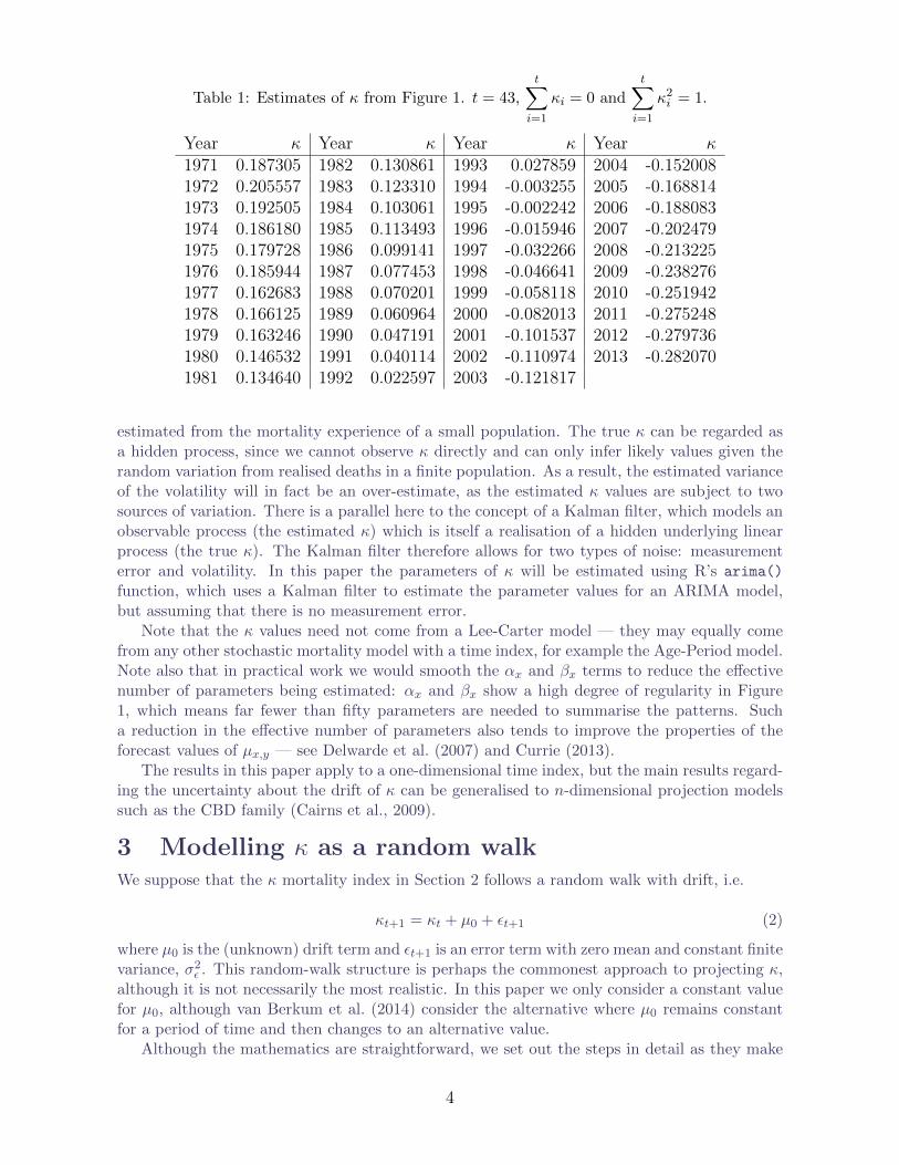
different constraint systems produce different parameter values, but the same fitted values forlogµx,y. The resulting parameter estimates are shown in Figure 1, with the estimated valuesfor κ in Table 1. It is these κ values which must be projected, and this paper is about (i) theoptions available for forecasting κ, (ii) the uncertainty over these projections, and (iii) how theuncertainty may be decomposed into various sources of risk.
Figure 1: Parameter estimates for Lee-Carter model fitted to mortality data for malesin England & Wales aged 50–104 over the period 1971–2013.
60 80 100
−4
−2
Age
αx
60 80 100
0
1
2
Age
βx
1980 2000
−0.2
0
0.2
Year
κy
The κ values will be treated throughout this paper as if they are known quantities, butit is worth noting that this is a simplification; in fact, the κ values are themselves estimates,and there is thus uncertainty over their true underlying value, especially if the κ values are
3
Table 1: Estimates of κ from Figure 1. t = 43,t∑i=1
estimated from the mortality experience of a small population. The true κ can be regarded asa hidden process, since we cannot observe κ directly and can only infer likely values given therandom variation from realised deaths in a finite population. As a result, the estimated varianceof the volatility will in fact be an over-estimate, as the estimated κ values are subject to twosources of variation. There is a parallel here to the concept of a Kalman filter, which models anobservable process (the estimated κ) which is itself a realisation of a hidden underlying linearprocess (the true κ). The Kalman filter therefore allows for two types of noise: measurementerror and volatility. In this paper the parameters of κ will be estimated using R’s arima()
function, which uses a Kalman filter to estimate the parameter values for an ARIMA model,but assuming that there is no measurement error.
Note that the κ values need not come from a Lee-Carter model — they may equally comefrom any other stochastic mortality model with a time index, for example the Age-Period model.Note also that in practical work we would smooth the αx and βx terms to reduce the effectivenumber of parameters being estimated: αx and βx show a high degree of regularity in Figure1, which means far fewer than fifty parameters are needed to summarise the patterns. Sucha reduction in the effective number of parameters also tends to improve the properties of theforecast values of µx,y — see Delwarde et al. (2007) and Currie (2013).
The results in this paper apply to a one-dimensional time index, but the main results regard-ing the uncertainty about the drift of κ can be generalised to n-dimensional projection modelssuch as the CBD family (Cairns et al., 2009).
3 Modelling κ as a random walkWe suppose that the κ mortality index in Section 2 follows a random walk with drift, i.e.
κt+1 = κt + µ0 + εt+1 (2)
where µ0 is the (unknown) drift term and εt+1 is an error term with zero mean and constant finitevariance, σ2ε . This random-walk structure is perhaps the commonest approach to projecting κ,although it is not necessarily the most realistic. In this paper we only consider a constant valuefor µ0, although van Berkum et al. (2014) consider the alternative where µ0 remains constantfor a period of time and then changes to an alternative value.
Although the mathematics are straightforward, we set out the steps in detail as they make
4
a useful comparison for the ARIMA model in Section 4. Under the random-walk model, therealised values of κt+h (h steps ahead) are given by:
κt+h = κt + hµ0 +
h∑j=1
εt+j (3)
Assuming for the moment that µ0 is known, and given the value for κt, we obtain a centralforecast h years ahead, κt(h), by setting all the error terms εt+j to zero, i.e.
κt(h) = κt + hµ0 (4)
However, since µ0 is unknown we replace it with an estimate, µ0, which is derived as follows:
µ0 =1
t− 1
t∑i=2
(κi − κi−1) =κt − κ1t− 1
(5)
where t is the number of κ terms (t = 43 in Table 1). In equation (5) we estimate µ0 using anunbiased estimator µ0 which coincides with the MLE for the mean of the Normal distribution(and for the mean of many other distributions besides).
Equations (4) and (5) gives us a forecast estimator h years ahead, κt(h):
κt(h) = κt + hµ0 (6)
For the variance of µ0 we have:
Var(µ0) = Var
(κt − κ1t− 1
)
=1
(t− 1)2Var
κ1 + (t− 1)µ0 +t∑
j=2
εj − κ1
=
σ2εt− 1
(7)
For the data in Table 1 we obtain µ0 = −0.011176. Our estimate of σ2ε is the appropriatesample variance, σ2ε :
σ2ε =1
t− 2
t∑i=2
(κi − κi−1 − µ)2 (8)
which gives σ2ε = 0.00011 (σε = 0.010512). Technically σ2ε is also a parameter being estimated,and there is uncertainty over this estimate. However, for the purposes of this paper we areconcerned with parameter risk which affects the trend. The estimated standard error of µ0 istherefore 0.001622.
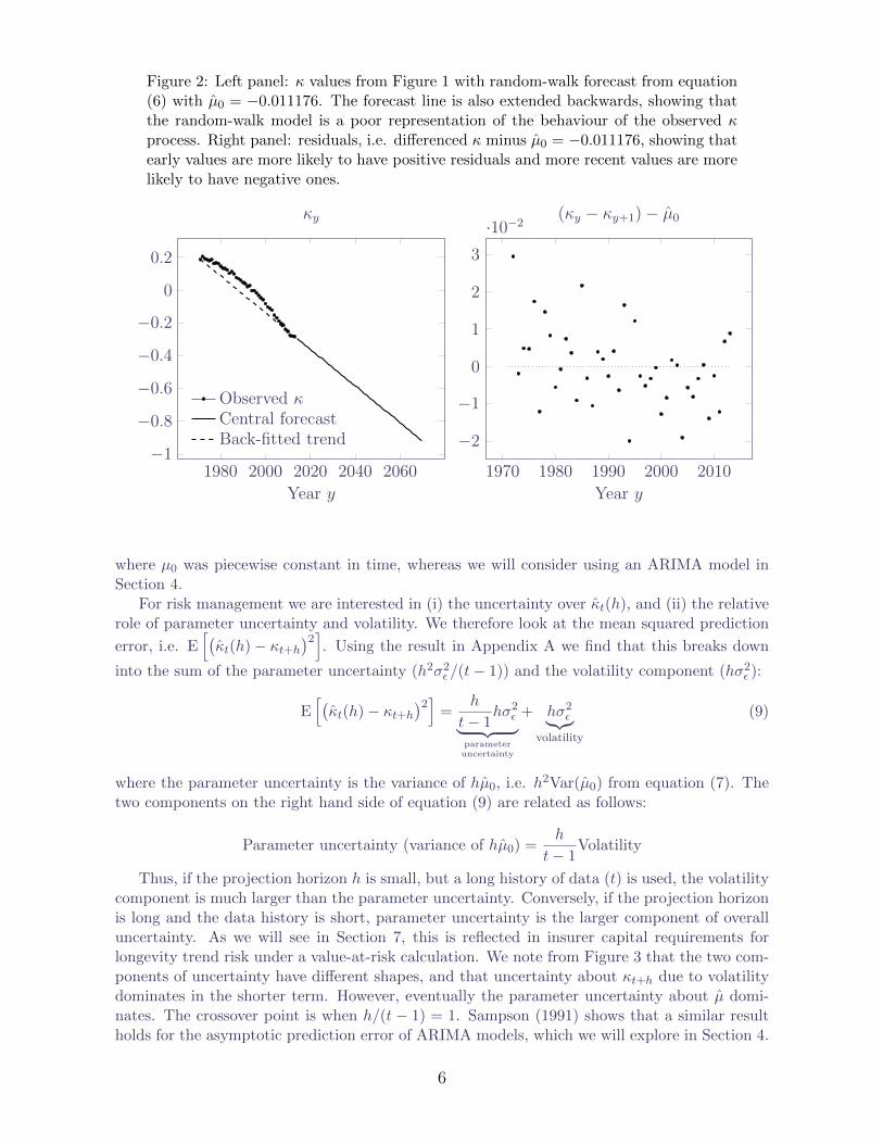
The resulting central forecast, κt(h), defined in equation (6) is depicted in Figure 2, wherewe can see that the random-walk process is a poor representation of the past behaviour of κ. Asshown in equation (5), the random walk with drift just draws a line between the first and last κterms, ignoring the non-linear pattern in between. This is not a unique finding — van Berkumet al. (2014) noted a similarly poor fit to modern Dutch data using a Lee-Carter model. Wetherefore need to find a better model; van Berkum et al. (2014) used a random walk with drift
5
Figure 2: Left panel: κ values from Figure 1 with random-walk forecast from equation(6) with µ0 = −0.011176. The forecast line is also extended backwards, showing thatthe random-walk model is a poor representation of the behaviour of the observed κprocess. Right panel: residuals, i.e. differenced κ minus µ0 = −0.011176, showing thatearly values are more likely to have positive residuals and more recent values are morelikely to have negative ones.
1980 2000 2020 2040 2060−1
−0.8
−0.6
−0.4
−0.2
0
0.2
Year y
κy
Observed κCentral forecastBack-fitted trend
1970 1980 1990 2000 2010
−2
−1
0
1
2
3
·10−2
Year y
(κy − κy+1)− µ0
where µ0 was piecewise constant in time, whereas we will consider using an ARIMA model inSection 4.
For risk management we are interested in (i) the uncertainty over κt(h), and (ii) the relativerole of parameter uncertainty and volatility. We therefore look at the mean squared prediction
error, i.e. E[(κt(h)− κt+h
)2]. Using the result in Appendix A we find that this breaks down
into the sum of the parameter uncertainty (h2σ2ε /(t− 1)) and the volatility component (hσ2ε ):
E[(κt(h)− κt+h
)2]=
h
t− 1hσ2ε︸ ︷︷ ︸
parameteruncertainty
+ hσ2ε︸︷︷︸volatility
(9)
where the parameter uncertainty is the variance of hµ0, i.e. h2Var(µ0) from equation (7). Thetwo components on the right hand side of equation (9) are related as follows:
Parameter uncertainty (variance of hµ0) =h
t− 1Volatility
Thus, if the projection horizon h is small, but a long history of data (t) is used, the volatilitycomponent is much larger than the parameter uncertainty. Conversely, if the projection horizonis long and the data history is short, parameter uncertainty is the larger component of overalluncertainty. As we will see in Section 7, this is reflected in insurer capital requirements forlongevity trend risk under a value-at-risk calculation. We note from Figure 3 that the two com-ponents of uncertainty have different shapes, and that uncertainty about κt+h due to volatilitydominates in the shorter term. However, eventually the parameter uncertainty about µ domi-nates. The crossover point is when h/(t − 1) = 1. Sampson (1991) shows that a similar resultholds for the asymptotic prediction error of ARIMA models, which we will explore in Section 4.
6
Figure 3: κ values with forecast from random walk with drift with (i) 95% bounds forparameter uncertainty and (ii) stochastic volatility. Panel (iii) shows the relationshipbetween the two sources of uncertainty over the course of the projection. Note thewider range in panel (iv), reflecting the wider interval arising from including bothsources of uncertainty.
1980 2000 2020 2040 2060
−1
−0.5
0
(i) Uncertainty about µ.
Observed κCentral forecast95% bound
1980 2000 2020 2040 2060
−1
−0.5
0
(ii) Uncertainty from volatility.
Observed κCentral forecast95% bound
2010 2020 2030 2040 2050 2060 2070−1.2
−1
−0.8
−0.6
−0.4
−0.2
(iii) Uncertainty about µ v.uncertainty from volatility.
Parameter onlyVolatility only
2010 2020 2030 2040 2050 2060 2070−1.2
−1
−0.8
−0.6
−0.4
−0.2
(iv) Uncertainty about µand volatility combined.
4 Modelling κ as an ARMA or ARIMA processWe saw in Section 3 that the forecast uncertainty for a random walk with drift could be splitinto two components: parameter uncertainty and volatility. However, we also saw in Figure 2that a random walk with drift was a poor representation of the historical pattern of κ. As wewill see, κ is better represented as an ARIMA process, and the forecast uncertainty of such aprocess can be analogously decomposed into parameter uncertainty and volatility.
We begin by defining an ARMA(p,q) process, X0t , with zero mean:
X0t = ar1X
0t−1 + . . .+ arpX
0t−p +ma1εt−1 + . . .+maqεt−q + εt (10)
where εt is a series of independent, identically distributed error terms with zero mean andconstant finite variance, σ2ε . The p autoregressive parameters and q moving-average parameters
7
are to be estimated, and there will be uncertainty over these estimates which will contribute tothe overall forecast uncertainty. Moreover, there is also uncertainty about p and q which definethe model within the class of ARMA(p,q) processes. We will discuss the impact of choosingspecific values for p and q in Section 9 when we discuss model uncertainty. However, we restrictourselves to the family of stationary ARMA(p, q) processes for any orders p and q that weconsider.
Having defined the ARMA(p, q) process with a zero mean in equation (10), we can now useit to define an ARMA(p, q) process with a non-zero mean, µ:
X = X0 + µ (11)
As in Section 3, we can calculate an estimate of the mean, µ:
µ = X =1
t
t∑i=1
Xi (12)
Since X is a stationary ARMA process, we have E[µ] = µ. Furthermore, using the derivationin Appendix B we have the following result for the variance of µ:
Var (µ) =Var(X0)
t+
2
t
t−1∑k=1
γ(k)
[1− k
t
](13)
where γ(k) = Cov(Xt, Xt+k) is the auto-covariance function of X. Note that γ(0) = Var(X0t )
by definition. Also note that (13) reduces to (7) if X is a sequence of independent randomvariables, since γ(k) = 0 for all k 6= 0 in this case.
Asymptotically, we obtain for t→∞:
tVar (µ)→∞∑
k=−∞γ(k) (14)
if∑∞
k=−∞ |γ(k)| <∞, see Appendix B and also Theorem 7.1.1 in Brockwell and Davis (1987).Comparing equations (7) and (13) we see that the variance of µ can be either higher or lower
than the variance of the estimated mean µ0 of a sequence of independent random variables.Any dependencies between observations Xt and Xt+k can therefore either increase or decreasethe uncertainty about µ, depending on whether
∑t−1k=1 γ(k)
[1− k
t
]is positive or negative. For
example, an AR(1) model with a negative autoregressive parameter would have lower parameteruncertainty (about the mean) than a model where X0 is a sequence of independent variables.
In empirical studies the autocovariance function γ(k) in equation (13) is not known. There-fore, the variance of µ needs to be estimated. We compared the accuracy of three differentapproaches to obtain an estimate for Var (µ). In our first approach we replaced γ(k) by thesample autocovariances obtained from observed values of X. We found in simulation studiesthat the estimated values of γ(k) for large values of k were unreliable (the estimator γ(k) has alarge variance) and therefore, the estimated value of Var (µ) was also unreliable. An alternativeapproach is to fit an ARMA model to X and then use the theoretical autocovariance functionγ(k) based on the estimated parameters of the fitted ARMA model. We found that this ap-proach provided reasonable estimates of Var (µ). However, while this second approach will giveus the variance for µ, it will not give us information on possible extreme values. In insurancework we are primarily interested in extreme quantiles like the 99.5% point, so in our empiricalstudy in Sections 5 and 6 we adopted a third approach: we used a parametric bootstrap proce-dure to obtain the full distribution, and in particular, the variance of µ directly from bootstrap
8
realisations of µ without the need to find the autocovariance function γ(k) of X first. This thirdapproach was used for consistency in the treatment of uncertainty over the ARMA parametersand µ, but also in generating a full distribution for the exploration of extremes. We will see theimportance of this in Section 5.
We also note that the estimator µ = X is not the maximum-likelihood estimator for µunless the ARMA process is a sequence of independent random variables. In general, the MLEfor µ will depend on the (estimated) ARMA parameters. To illustrate this point we show thederivation of the MLE for µ for an AR(p) process in Appendix D (see also Harvey (1981) forthe case for an AR(1) process). We find that the MLE is very close to the mean X for smallvalues of p. Furthermore, both estimators are unbiased. However, since the MLE for µ dependson the estimated ARMA parameters and the order of the ARMA model, different estimatesfor µ will be obtained when the order of the model is changed. We therefore argue that themean µ = X is a more robust alternative to the MLE. Being able to estimate µ independentlyof other parameters also has the advantage that the process X0 can be fitted to appropriatemodels using maximum likelihood, least squares or other methods without re-estimating µ. Forall these reasons we prefer µ = X compared to the MLE for µ. A short discussion of the meancompared to the best linear unbiased estimator (BLUE) can be found in Brockwell and Davis(1987, p213). They argue that since the asymptotic variances in equation (14) are equal forboth estimators, they use the simple estimator µ.
Although using the sample mean X as an estimator for µ means that the estimated valueof µ will be independent of the fitted ARMA model, the estimated standard error of µ willdepend on the chosen ARMA model and the fitted parameters since we do not use the empiricalautocovariances in equation (13) for the reasons explained earlier.
We can thus model the period effect κ in our Lee-Carter model as an ARMA(p, q) processby setting κ = X. Alternatively, and more realistically, we can model κ as an ARIMA(p, 1, q)process:
κt = κt−1 +Xt = κt−1 +X0t + µ ∀ t > 1 (15)
where κ1 is a given constant or a random variable independent of the process X. The realisedvalue of κ, h steps ahead, is as follows:
κt+h = κt+h−1 +Xt+h
= κt+h−1 +X0t+h + µ
= κt+h−2 +X0t+h−1 +X0
t+h + 2µ
...
= κt +
h∑i=1
X0t+i + hµ (16)
with X0t+h given by equation (10). It is possible to model κ using an ARIMA(p, d, q) process
with d > 1, but we will restrict our attention to d = 1 here. Note that with d = 1 we aremodelling improvements in κ, i.e. relative changes, whereas with d = 2 we would be modellingchanges in the rate of improvement, i.e. acceleration or deceleration in improvements.
We can now define h-step ahead projections for κ as in the previous section, that is:
κt(h) = κt +h∑i=1
X0t+i + hµ
κt(h) = κt +h∑i=1
X0t+i + hµ
9
where we set all error terms εt+h = 0 for all h > 0 in equation (10) to obtain projected values forX0, and we define X0 as in equation (10) but with the coefficients ai and bi, and the residualsε up to time t being replaced by their estimated values.
The ARIMA model is a generalisation of the random-walk model — in each case µ0 (fora random walk with drift) and µ (for an ARIMA model) play analogous roles. However, it isinteresting to note how quickly µ can come to dominate the projected κt(h) for an ARIMAmodel, i.e. where the ε values are set to zero for the central forecast. For example, in anARIMA(0,1,q) model the influence of the last observed ε terms ceases after q + 1 years, as perequation (10). Similarly, the closer the autoregressive parameters are to zero, the quicker µdominates the forecast as we discuss in detail in Section 9. Since the impact of these moving-average and autoregressive parameters can be quickly dominated by µ, it suggests that theuncertainty over them might also be dominated by the uncertainty over µ.
5 Fitting an ARIMA model for κTo fit an ARIMA model we need to make a choice over the values of p, d and q. In theremainder of this paper we will set d = 1 and consider values of p and q in {0, 1, 2, 3}. Weapply maximum-likelihood estimators as implemented in the statistical software R, see R CoreTeam (2012), to obtain estimated values of the coefficients ai and bi in equation (10). We thenuse the information criterion from Akaike (1987) with the small-sample correction from Hurvichand Tsai (1989) to select our final model. Table 2 shows the AICc values when the variousARIMA(p, 1, q) models are fitted to the data in Table 1, showing that the best-fitting model isARIMA(1,1,2). The same model is selected if we target the BIC or the AIC without the small-sample correction. The estimated parameter values for the ARIMA(1,1,2) model are shown inTable 3.
Table 2: AICc values for various ARIMA(p, 1, q) models.
Table 3: Parameter estimates for ARIMA(1,1,2) model fitted to κ values in Table 1.Source: arima() function in R Core Team (2012) for ar1, ma1, ma2 and σ2ε , equations(12) and (13) for µ.
As mentioned earlier the estimate for µ is obtained using (12) rather than the maximumlikelihood estimator implemented in R’s arima function. The reported standard error for µ is
10
therefore not based on the information matrix of the MLE, but on a bootstrap sample whichwe explain below. Also, while we are comfortable enough with the estimated values in Table 3,we are less comfortable with the standard errors: for example, adding more than one standarderror to ar1 would make the process non-stationary. As an alternative to these standard errors,we use bootstrapping to investigate the finite-sample distribution of ar1, ma1, ma2 and σ2ε (seeFigure 5).
The forecast for the model in Table 3 is shown in Figure 4, together with the residuals.Figure 4 can be compared and contrasted directly with Figure 2. The first point of note isthat the residuals look better for the ARIMA(1,1,2) model: not only are the ARIMA residualssmaller with a narrower range, but the ARIMA residuals are better distributed over time. TheARIMA model is clearly a better fit. The second point of note is that the central forecast seemsto be a more natural extrapolation of the historical κ values. In particular, there is a visiblecurvature to the central forecast, which arises from the autoregressive component of the ARIMAmodel.
Figure 4: Left panel: κ values from Figure 1 with ARIMA(1,1,2) forecast from Table3. Right panel: residuals from the ARIMA fit.
1980 2000 2020 2040 2060
−1
−0.5
0
Year
κy
Observed κCentral forecast
1970 1980 1990 2000 2010
−1
0
1
2
·10−2
Year
Residuals
Having established that an ARIMA model is both a better fit to the κ process and seemsto be a more natural extrapolation than a random walk with drift, we now turn to the subjectof parameter uncertainty. Appendix C shows the decomposition of forecast uncertainty in anARIMA model into (i) parameter uncertainty (the variance of µ, the variance of the autoregres-sive terms and the variance of the moving-average terms) and (ii) volatility. We are interestedin the variance contributions for the various parameters, but, as noted in Appendix C, there areno closed-form expressions for the uncertainty over the parameters.
Instead, we use the bootstrap methodology described by Pascual et al. (2004). For a givenARIMA(p, d, q) model and fitted parameters, the approach is to take a short sample of thetime series and simulate further values assuming the fitted parameters are known with certainty(we are only using d = 1 in this paper). The length of the simulated extension is such thatthe length of the new sequence — the fixed values plus the newly simulated values — is thesame length as the original sample. An ARIMA model with the same order is fitted to the newsequence, i.e. new parameter values are estimated. The process is repeated 1,000 times, say,and the resulting distribution of each parameter value is the bootstrap estimate.
Following Pascual et al. (2004) our bootstrap procedure therefore consists of the following
11
steps, assuming that we have observed the process κ for T + 1 years, i.e. we have observationsκ0, . . . κT :
1. define Xt = κt − κt−1, estimate µ with µ = X and define X0t = Xt − µ for t = 1, . . . , T
2. fit an ARMA(p,q) model to obtain the vector θ0 = (ar1, . . . , arp, ma1, . . . , maq, σ2ε) of
estimated parameters where ari and mai are the estimates for the parameters ari and maiin equation (10) and σ2ε is the estimated variance of εt; the estimated parameters for ourdata are given in Table 3
3. simulate N trajectories of an ARMA(p,q) process according to (10) with parameter vectorθ0; each trajectory X(k) = {X1(k), . . . , XT (k)} for k = 1, . . . , N is of length T startingfrom initial values x1(k), . . . , xp(k); and initial residuals ε1(k), . . . , εq(k); all other residualsare drawn from a normal distribution N(0, σ2ε)
4. estimate the parameter vector θ for each simulated trajectory to obtain the estimatedparameter vector θ(k) for trajectory k; also estimate the mean as µ(k) = X(k) to obtainbootstrap realisations of µ which we then use to calculate its variance as mentioned insection 4 since the autocovariance function γ in equation (13) is not observed.
Pascual et al. (2004) used the same initial fixed sequence for each simulation in step 3, i.e.x1(k), . . . , xp(k) and ε1(k), . . . , εq(k) in step 3 do not depend on k. In contrast, here we haverandomly sampled a contiguous segment of the time series X to avoid any dependency on thechoice of the fixed initial sequence. It might strike readers as unusual to not use the most recentκ values as the fixed sequence in this bootstrap procedure, but the log-likelihood in Harvey(1981, p122, equation 2.2) shows that this should have a small impact on the estimation of theautoregressive and moving-average parameters. The choice of a fixed initial sequence can havea material impact on the estimation of σ2ε , however, as shown later in the comparison of Figures8 and 9. The resulting bootstrap estimates for the distributions of the parameters are shown inFigure 5.
In our empirical example we consider bootstrap samples with a sample size N = 1, 000. Wefound that some to the trajectories simulated in step 3 of the above bootstrap procedure do notseem to correspond to a stationary ARMA(p, q) model, and therefore R’s arima function fails toestimate the parameters. For this reason, some of the resulting bootstrap samples contain lessthan 1,000 simulated realisations of the estimated paramter values. Nonparametric estimatesof the densities of the resulting bootstrap sample are shown in Figure 5 for the parameters ofthe ARIMA(1,1,2) model fitted to the observed period effect κ. For this specific example wefound that two out of the 1,000 simulated trajectories for X do not correpond to a stationaryARMA(1,2) process, that is, the effective number of simulated trajectories is N=998.
We can use the results from Figure 5 to investigate the relative contribution to uncertaintyfrom each source: (i) uncertainty over µ, (ii) uncertainty over the ARMA parameters, (iii)uncertainty from volatility and (iv) uncertainty from volatility including uncertainty over thevalue of σ2ε . These four cases are plotted in Figure 6. The bottom two panels show that there isno practical difference from considering the uncertainty over σ2ε , i.e. the estimate of σ2ε in Table3 is all we need to consider for the volatility.
Figure 6 reveals a number of important differences when compared with the relevant panels inFigure 3 for a random walk with drift. One feature is the different initial shape of the confidencebounds for volatility only: with the random-walk model, there is an immediate bulge in the firstyear of projection in Figure 3(ii), whereas for the ARIMA(1,1,2) model the first year shows nosuch bulge in Figure 6(ii). The reason lies in the contrast between structures of the models.Consider equation (9) for the random walk: with no parameter risk the first term is zero and sothe variance of the random-walk forecast is linear in terms of the projection horizon, h. This is
12
Figure 5: Estimated densities of ar1, ma1, ma2 and σ2ε parameters for ARIMA(1,1,2)model fitted to data in Table 1. The dashed vertical lines show the estimated values foreach parameter from Table 3. Density estimation is done according to the procedurefrom Pascual et al. (2004).
ar1
N = 1000 Bandwidth = 0.1009
−1.0 −0.5 0.0 0.5 1.0
0.0
0.5
1.0
1.5
2.0
ma1
N = 1000 Bandwidth = 0.1129
−2 −1 0 1
0.0
0.2
0.4
0.6
0.8
1.0
1.2
1.4
ma2
N = 1000 Bandwidth = 0.09718
−1.0 −0.5 0.0 0.5 1.0
0.0
0.5
1.0
1.5
σε2
N = 1000 Bandwidth = 3.781e−06
0.00002 0.00006 0.00010
0
5000
10000
15000
20000
25000
because the difference κt+h − κt involves the addition of h i.i.d. ε terms. This means that thestandard error of the forecast increases in line with
√h and this gives a rapid initial expansion of
the confidence interval, followed by slower expansion later on. The ARIMA model in equation(10) also has a projection which involves the addition of i.i.d. ε terms, but the structure ofthe model means that κt+h − κt is not the straightforward sum of these terms. The structureof the ARIMA model introduces correlations that are not present in the drift model, both viathe autoregressive and moving-average terms. These correlations mean that the variance of theforecast is not linear in terms of h, and so the standard error of the forecast does not behavelike√h.
In Figure 3(iii) we see that the parameter uncertainty over µ in a drift model eventuallydominates the uncertainty due to volatility. In contrast, a comparison of Figure 6(i) with eitherpanel (iii) or (iv) suggests that the uncertainty due to volatility remains dominant. Finally,
13
Figure 6: Forecast κ values from ARIMA(1,1,2) model in Table 3 with 95% boundsfor various kinds of uncertainty.
2020 2040 2060−1.5
−1
−0.5
(i) Uncertainty over µ only.
Forecast95% bound
2020 2040 2060−1.5
−1
−0.5
(ii) Uncertainty about the ar1,ma1 and ma2 parameters only.
Forecast95% bound
2020 2040 2060−1.5
−1
−0.5
(iii) Uncertainty from volatilityonly with σ2
ε as per Table 3.
Forecast95% bound
2020 2040 2060−1.5
−1
−0.5
(iv) Uncertainty from volatility withuncertainty around σ2
ε as per Figure 5.
Forecast95% bound
particular comment is required for Figure 6(ii); at first glance, the confidence interval lookswrong for the central projection — the confidence interval is nowhere near symmetric around thecentral projection, not even for the first year. However, there is no mistake — the strange-lookingconfidence bounds in relation to the central projection are a consequence of the highly skeweddistribution of the ar1 parameter in Figure 5. For the ARIMA(1,1,2) model, the largest singlecomponent of parameter uncertainty is the uncertainty over the ARMA parameters, particularlythe uncertainty over the ar1 parameter.
6 Alternative ARIMA models for κIn Section 5 we used an ARIMA(1,1,2) model because this produced the lowest AICc when fittedto the data (see Table 2). However, Figure 5 shows that the estimated parameter values arenot robust - the ar1 parameter in particular is close to 1, where values of 1 or more would makethe process X non-stationary. A consequence of this lack of robustness is the large impact ofthe uncertainty over the ar1, ma1 and ma2 parameters on simulated future mortality scenarios,as shown in in Figure 6(ii). This suggests that goodness of fit to past data should perhaps
14
not be the sole criterion for model selection. To illustrate this, we show some results for theARIMA(1,1,0) model, i.e. a pure integrated AR(1) model with drift term. Table 2 shows thatthis is a materially poorer fit to the past data than the ARIMA(1,1,2) model used in Section 5,and that the AICc is almost identical to the AICc of the random-walk model.
The estimated parameter values for the ARIMA(1,1,0) model are shown in Table 4. We notethat the estimated value for σ2ε is very similar to the estimated value of σ2ε in the random-walkmodel, which is in line with the very similar AICc values for those two models. This parameteris significantly smaller in the ARIMA(1,1,2) model indicating that the two moving-averageparameters improve the fit of the model. We also find that the estimated ar1 parameter is verydifferent from the estimated ar1-parameter in the ARIMA(1,1,2) model. This leads to a verydifferent behaviour of the central projection, as shown in Figure 7. Indeed, for the ARIMA(1,1,0)model we find that the ar1 parameter is rather close to zero, so that the uncertainty about thisparameter is not relevant for the uncertainty about the central mortality projection — seeFigures 8 and 10. The central projection for the ARIMA(1,1,0) model is almost identical to thecentral projection obtained with a random-walk model.
Table 4: Parameter estimates for ARIMA(1,1,0) model fitted to κ values in Table 1.Source: arima() function in R Core Team (2012) for ar1 and σ2ε , equation (12) forµ. The standard error of µ is obtained from the sample standard deviation of thebootstrap sample {µ(k), k = 1, . . . , N}.
Figure 7: Left panel: κ values from Figure 1 with ARIMA(1,1,0) forecast from Table4. Right panel: residuals from the ARIMA(1,1,0) fit.
1980 2000 2020 2040 2060−1
−0.8
−0.6
−0.4
−0.2
0
0.2
Year
κy
Observed κCentral forecast
1970 1980 1990 2000 2010
−2
−1
0
1
2
3
·10−2
Year
Residuals
15
Figure 8: Estimated densities of ar1 and σ2ε parameters for ARIMA(1,1,0) model fittedto data in Table 1. The dashed vertical lines show the estimated values for eachparameter from Table 4. Density estimation is done according to the procedure fromPascual et al. (2004).
ar1
N = 1000 Bandwidth = 0.0327
−0.8 −0.4 0.0 0.2
0.0
0.5
1.0
1.5
2.0
2.5
σε2
N = 1000 Bandwidth = 3.477e−06
0.00004 0.00010
0
5000
10000
15000
20000
25000
Figure 9: Estimated densities of ar1 and σ2ε parameters for ARIMA(1,1,0) model fittedto data in Table 1. The dashed vertical lines show the estimated values for eachparameter from Table 4. In contrast to Figure 8, the bootstrapping procedure ofPascual et al. (2004) is modified to randomly select initial sub-series from the data; acomparison with Figure 8 shows that this has reduced the bias for σ2ε .
ar1
N = 1000 Bandwidth = 0.03548
−0.8 −0.4 0.0 0.4
0.0
0.5
1.0
1.5
2.0
2.5σε
2
N = 1000 Bandwidth = 3.606e−06
0.00006 0.00010 0.00014
0
5000
10000
15000
20000
25000
16
Figure 10: κ values with forecast from ARIMA(1,1,0) model with 95% bounds forvarious kinds of uncertainty.
2010 2020 2030 2040 2050 2060 2070−1.2
−1
−0.8
−0.6
−0.4
−0.2
(i) Uncertainty over µ only.
Forecast95% bound
2010 2020 2030 2040 2050 2060 2070−1.2
−1
−0.8
−0.6
−0.4
−0.2
(ii) Uncertainty about the ar1parameter only.
Forecast95% bound
2010 2020 2030 2040 2050 2060 2070−1.2
−1
−0.8
−0.6
−0.4
−0.2
(iii) Uncertainty from volatilityonly with σ2
ε as per Table 4.
Forecast95% bound
2010 2020 2030 2040 2050 2060 2070−1.2
−1
−0.8
−0.6
−0.4
−0.2
(iv) Uncertainty over µ v.uncertainty from volatility
Parameter onlyVolatility only
7 Impact on value-at-risk-style capital requirementsThe confidence intervals in Figures 3 and 6 are based on a run-off approach to projection.However, under the Solvency II regulatory regime in the European Union, insurers using internalmodels need to calculate reserves using a one-year, value-at-risk (VaR) approach. In this sectionwe look at the impact of the various sources of uncertainty on capital requirements calculatedusing the VaR methodology of Richards et al. (2014). The VaR methodology involves using thefitted projection model to repeatedly simulate one year’s additional mortality experience, thenrefitting the model and using the resulting updated central forecast to value an annuity liability.
For each of 1,000 VaR simulations we simulate the extra year’s experience using three al-ternative combinations. The first option (labelled “Volatility only” in Table 5) means σ2ε is setto its estimated value and one new ε error term is simulated for the moving-average processfor each of the 1,000 simulations; all other parameters — ARMA parameters and the mean —are fixed at their estimated values and there is no parameter uncertainty. The second option
17
(labelled “Trend risk only” in Table 5) means the ARMA parameters and the mean (drift) termcome from a single bootstrap realisation; σ2ε is set to zero and there is therefore no volatilityin the moving-average process. The third option (labelled “Trend risk and volatility combined”in Table 5) means the ARMA parameters and the mean term come from a single bootstraprealisation, together with σ2ε set to its estimated value and one error term simulated for themoving-average process. Splitting the sources of uncertainty in this way allows us to examinethe size of the various contributions made to the overall capital requirements.
The results for a value-at-risk assessment of longevity trend risk are given in Table 5. Wehave used a Lee-Carter model without smoothing fitted to the mortality data for males aged50–104 in England & Wales over 1971–2013. All ARIMA models have been fitted with a non-zero mean. The factors in Table 5 are for temporary, continuously-paid annuities to a single lifeaged 70 at outset, with cashflows discounted at 2.5% per annum.
Table 5: Sensitivity of VaR capital requirements to various ARIMA models and thesources of uncertainty included. There is one bootstrap realisation of the ARMA and µparameters per VaR calculation, but not all bootstrap realisations produce stationarymodels.
ARIMA(0,1,0) 1000 Yes No 12.50 12.70 1.62%1000 No Yes 12.50 12.54 0.33%1000 Yes Yes 12.49 12.72 1.79%
ARIMA(0,1,1) 1000 Yes No 12.51 12.68 1.32%1000 No Yes 12.51 12.56 0.34%1000 Yes Yes 12.51 12.69 1.44%
ARIMA(1,1,0) 1000 Yes No 12.51 12.68 1.36%1000 No Yes 12.51 12.55 0.31%1000 Yes Yes 12.51 12.69 1.43%
ARIMA(1,1,1) 1000 Yes No 12.50 12.67 1.37%1000 No Yes 12.51 12.56 0.37%1000 Yes Yes 12.51 12.69 1.44%
ARIMA(1,1,2) 1000 Yes No 12.59 12.87 2.25%994 No Yes 12.53 12.61 0.63%994 Yes Yes 12.53 12.87 2.70%
Table 5 shows that for many simple models the uncertainty over the ARMA parametervalues and the mean makes only a modest additional contribution to the capital requirements.Value-at-risk calculations are driven by the variability of mortality experience over a one-yearhorizon and how the model fit responds to this. The reason why the volatility makes the largestcontribution in Table 5 is the same point as made at the end of Section 3 for the random walk:the relative influence of volatility and parameter risk depends on the projection horizon andthe length of the data series. In the case of VaR calculations, the projection horizon is just oneyear, thus maximising the influence of the volatility. This applies even for the ARIMA(1,1,2)model, where the parameter uncertainty shown in Figure 6 is very large. In contrast to theother models in Table 5, the parameter uncertainty of the ARIMA(1,1,2) model in Figure 6(ii)leads to a material additional capital requirement. This is perhaps surprising for the modelwhich best fits the data, as demonstrated by Table 2. However, Table 5 gives another hintas to why the ARIMA(1,1,2) produces the greatest capital requirements: it is the only model
18
where the bootstrapped ARMA parameter values sometimes produced non-stationary models,as evidenced by the reduced number of usable parameter sets from bootstrap simulation (994instead of 1,000). The ARIMA(1,1,2) model might fit the data best, but it is less stable andproduces higher capital requirements as a result.
8 Comparison with CMI projectionsThe CMI is the part of the UK actuarial profession that produces reference mortality tables andoccasional mortality forecasts for use by insurers and pension schemes. One such forecastingtool is described in Continuous Mortality Investigation (2009), and it has been updated moreor less annually since. This tool takes the form of an Excel spreadsheet and it is in wide usethroughout the UK, both for annuity portfolios and pension schemes.
The CMI spreadsheet works with relative mortality-improvement rates, rather than mortalityrates. A mortality improvement is defined as 1 − qx,t/qx,t−1, where qx,t is the probability thatan individual alive aged x at the start of year t will die before the end of the year. See Willets(1999) for more detailed discussion of mortality improvements in insured portfolios and thewider population.
The CMI spreadsheet operates by user input of the assumed long-term rate of mortalityimprovement and the current rates of mortality improvement are then blended towards thisvalue. There are over a thousand parameters which can be used by the user to customise therate of blending by calendar year, age or year of birth. The CMI spreadsheet is therefore adeterministic targeting method of projection, as opposed to a stochastic model with parametersset by fitting to experience data.
The setting of the long-term mortality-improvement rate in the CMI spreadsheet is donesubjectively, although some users set it with reference to average rates of improvement in therelevant population. We can relate this long-term rate to the means of the models in this paperas follows:
1− qx,tqx,t−1
≈ 1− µx,tµx,t−1
= 1− eαx+βxκt
eαx+βxκt−1From equation(1)
= 1− eβx(κt−κt−1)
= 1− [1 + βx(κt − κt−1) + . . .] Expanding exas a Maclaurin series
≈ −βx(κt − κt−1) (17)
Using equation (2), the approximate mortality improvement in equation (17) becomes−βx(µ0+εt), which has expected value−βxµ0. The mean of a random walk model, µ0, could therefore onlybe appropriate for setting the long-term improvement rate in the CMI projection when it is mod-ulated by the appropriate value of βx. From Figure 1 we see that βx > 2,∀x ∈ {54, 55, . . . , 75}.Using µ0 = −0.011176, a best-estimate long-term rate for the CMI spreadsheet using therandom-walk model would therefore be in excess of 2% for ages 50–78 inclusive, although theappropriate long-term rate declines sharply for higher ages: it is under 1% for ages over 89 andis effectively zero by age 100. A stressed value of the long-term rate for reserving purposes couldbe obtained by adding the appropriate number of standard errors to µ0. However, whetherit makes sense to take a parameter from a random-walk model and use it as a parameter forthe CMI spreadsheet is a matter for actuarial judgement, especially in conjunction with thethousand other parameters which can be varied.
19
9 DiscussionWe have considered three ARIMA(p,1,q) models for the period effect κ in the previous sections:ARIMA(0,1,0) (the random-walk model), ARIMA(1,1,2) and ARIMA(1,1,0). All three seem tobe reasonable models to use for generating scenarios for future mortality. In this section wediscuss some of the advantages and disadvantages that each model offers, focusing in particularon the impact of the selected model on mortality projections.
All three models have in common that they are integrated of order one, and therefore, thefirst difference of κ is modelled as a stationary process with a non-zero mean. If follows thatthe improvement rate of projected mortality rates will eventually approach this mean. However,the models differ significantly in the speed with which the improvement rate converges to thislong term value. The autoregressive coefficient, ar1, in equation (10) plays a central role forthe behaviour of mortality projections. For a random-walk model we have ar1 = 0, and for theother two models the estimated values of ar1 are reported in Tables 3 and 4.
The importance of ar1 can be seen when central projections are considered, i.e. where weset future error terms ε to zero. The projected values X0
t (h) based on the model in equation(10) and observations up to time t are then given by:
h ARIMA(0,1,0) ARIMA(1,1,0) ARIMA(1,1,2)
1 X0t (1) = ar1X
0t X0
t (1) = ar1X0t +ma1εt +ma2εt−1
2 X0t (2) = ar21X
0t X0
t (2) = ar1X0t (1) +ma2εt
> 2 X0t (h) = arh−21 X0
t (2)
Therefore, if ar1 = 0 (the random-walk model) then X0t (h) = 0 for all values of h. For the
other two models, long-term projections depend on the value of ar1 and the two-years-aheadforecast X0
t (2) which in turn is determined by the last observations of κ. Consequently, if ar1 israther large (ar1 ≈ 1) the central projection of X0 converges slowly to zero, and the incrementof κ tends to µ only very slowly. This is the case for the ARIMA(1,1,2) model, and it can beseen in Figure 4 that the decrease in κ is stronger for the first few projected values and only forlonger term projections κ behaves like a linear function with slope µ. On the other hand, theestimated ar1 parameter is rather small for the ARIMA(1,1,0) model and, therefore, the impactof past κ values on central projections vanishes very quickly, see the virtually linear projectionof κ in figure 7.
Turning to a quantitative comparison of the proposed models, we start with the randomwalk model in Section 3 and the ARIMA(1,1,0) model in Section 6. We note that the AICcvalues for those two models in Table 2 are almost identical. In addition, the central projectionsshown in Figures 2 and 7 are very similar and can be considered identical for practical purposes.Moreover, the uncertainty about ar1 in equation (10) has no significant impact on the widthof the prediction interval for κ as can be seen in Figure 10. The reason for those similaritiesis that the estimated ar1 is rather close to zero. As a result, the process X0 in equation (10)converges very quickly to zero when the error terms are set to zero, as can be seen from the aboveformulae for the central projections. However, comparing the difference between the width ofthe prediction intervals in Figures 3(iii) and 10(iii) we find that volatility is less important in theARIMA(1,1,0) model compared to the random-walk model, and that therefore, the uncertaintyabout the drift becomes the leading source of uncertainty for relatively short forecast horizons.
In contrast to the rather similar random-walk and ARIMA(1,1,0) models, the ARIMA(1,1,2)model behaves very differently. The estimated ar1 is close to 1, showing that the inclusion ofmoving-average terms has a significant impact on the estimated value of ar1 in equation (10).The convergence of X0 to its long term mean 0 is therefore much slower with a large value of
20
ar1. As a result, the projected value of X0t (h) depends on the two-steps-ahead forecast X0
t (2),which is the last projected value still depending on the MA-parameters. Therefore, since theestimated ar1 is rather large, uncertainty about this parameter, but also the last observed valuesof κ have a strong impact on long term projections in the ARIMA(1,1,2) model.
This raises questions about the robustness of the central projection of the ARIMA(1,1,2)model. From the density plot for ar1 in Figure 5 we observe that the bootstrap realisations of theestimator ar1 are concentrated at values close to one with a rather small variance, which seemsto be particularly small compared to the variance of the same estimator in the ARIMA(1,1,0)model, see Figure 8. However, the above arguments show that even small variations in the ar1coefficient might have a substantial impact on the central projection of mortality rates sincear1 is close to 1. This observation is confirmed by the wide prediction intervals in Figure 6(ii)showing that projected mortality rates are very sensitive to changes in ar1.
The sensitivity of projected rates with respect to the last observed values of κ is best il-lustrated by considering the different central projections obtained when a small number ofobservations is removed from the sample. In Figure 11 we show the central projections obtainedfrom the complete sample y = 1971, . . . , 2013 and the central projections obtained when one,two or three years are removed from the end of the sample, that is κy is observed for y from 1971to 2012 (one year removed), 2011 (two years removed) or 2010 (three years removed). While thecentral projections obtained from subsamples do not change much if an ARIMA(1,1,0) model isconsidered, the changes of the central projections based on the ARIMA(1,1,2) are significant.
Figure 11: Sensitivity of central projections when up to three years are removed fromthe end of the sample. Left panel: ARIMA(1,1,2) model. Right panel: ARIMA(1,1,0)model.
1980 2000 2020 2040 2060
−1
−0.5
0
Year
Observed κCentral forecast
1980 2000 2020 2040 2060
−1
−0.5
0
Year
Observed κCentral forecast
We conclude that the inclusion of the two moving-average parameters improved the fit of themodel as measured by the AICc, but the robustness of mortality rate projections suffers. Thechoice of an appropriate time series model for κ is therefore a problem which requires actuarialjudgement and should be based on well defined objectives. If models are chosen with robustnessof projections as a selection constraint then the best fitting ARIMA(1,1,2) model should not bechosen. However, if only short term projections are required then the ARIMA(1,1,2) seems to bethe most appropriate of all time series models that we have considered, but one should be awarethat the improvement rate of projected mortality rates will be different from the estimated µ inthe short to medium term for that model.
21
10 ConclusionsIn this paper we showed how an ARIMA model can be a more realistic representation thana random walk with drift for the index of mortality. We found that in both cases the overallrisk can be decomposed into parameter uncertainty and volatility. In an ARIMA process formortality forecasting, we found that selecting a model on the basis of fit can lead to projectionswhere the uncertainty over the ARMA parameters is too material to ignore. Furthermore, theuncertainty over the ARMA parameters can lead to additional capital requirements for insurersunder a value-at-risk assessment mandated by Solvency II. For other, non-optimally fittingARIMA models the uncertainty from the ARMA parameters was negligible, and the impact oninsurer capital requirements was small.
AcknowledgmentsTorsten Kleinow acknowledges financial support from Netspar under project LMVP 2012.03.
ReferencesAkaike, H. (1987). Factor analysis and AIC. Psychometrica 52, 317–333.
Borger, M. (2010). Deterministic shock vs. stochastic value-at-risk: An analysis of the SolvencyII standard model approach to longevity risk. Blatter DGVFM 31, 225–259.
Brockwell, P. J. and R. A. Davis (1987). Time Series: Theory and Methods. Springer Verlag.
Brouhns, N., M. Denuit, and J. K. Vermunt (2002). A Poisson log-bilinear approach to theconstruction of projected lifetables. Insurance: Mathematics and Economics 31(3), 373–393.
Cairns, A., D. Blake, K. Dowd, and A. Kessler (2015). Phantoms never die: Living withunreliable mortality data. Journal of the Royal Statistical Society, Series A.
Cairns, A. J. G., D. Blake, K. Dowd, G. D. Coughlan, D. Epstein, A. Ong, and I. Balevich(2009). A quantitative comparison of stochastic mortality models using data from Englandand Wales and the United States. North American Actuarial Journal 13(1), 1–35.
Continuous Mortality Investigation (2009). User Guide for The CMI Mortality ProjectionsModel: ‘CMI 2009’. Continuous Mortality Investigation.
Currie, I. D. (2013). Smoothing constrained generalized linear models with an application tothe Lee-Carter model. Statistical Modelling 13(1), 69–93.
Delwarde, A., M. Denuit, and P. H. C. Eilers (2007). Smoothing the Lee-Carter and Poissonlog-bilinear models for mortality forecasting: a penalized likelihood approach. StatisticalModelling 7, 29–48.
Girosi, F. and G. King (2008). Demographic Forecasting. Princeton University Press.
Granger, C. W. J. and P. Newbold (1977). Forecasting Economic Time Series. Academic Press.
Harvey, A. C. (1981). Time Series Models. Philip Allan Publishers Limited.
Hurvich, C. M. and C.-L. Tsai (1989). Regression and time series model selection in smallsamples. Biometrika 76, 297–307.
22
Lee, R. D. and L. Carter (1992). Modeling and forecasting US mortality. Journal of the AmericanStatistical Association 87, 659–671.
Pascual, L., J. Romo, and E. Ruiz (2004). Bootstrap predictive inference for arima processes.Journal of Time Series Analysis 25 (4), 449–465.
Plat, R. (2011). One-year value-at-risk for longevity and mortality. Insurance: Mathematicsand Economics 49(3), 462–470.
R Core Team (2012). R: A Language and Environment for Statistical Computing. Vienna,Austria: R Foundation for Statistical Computing. ISBN 3-900051-07-0.
Richards, S. J. and I. D. Currie (2009). Longevity risk and annuity pricing with the Lee-Cartermodel. British Actuarial Journal 15(II) No. 65, 317–365 (with discussion).
Richards, S. J., I. D. Currie, and G. P. Ritchie (2014). A value-at-risk framework for longevitytrend risk. British Actuarial Journal 19 (1), 116–167.
Sampson, M. (1991). The effect of parameter uncertainty on forecast variances and confidenceintervals for unit root and trend stationary time-series models. Journal of Applied Economet-rics 6 (1), 67–76.
Shiryayev, A. N. (1984). Probability. Springer Verlag.
van Berkum, F., K. Antonio, and M. Vellekoop (2014). The impact of multiple structuralchanges on mortality predictions. Scandinavian Actuarial Journal 2014, 1–23.
Willets, R. C. (1999). Mortality in the next millennium. Staple Inn Actuarial Society, London.
23
Appendices
A Decomposition of forecast uncertainty for a ran-
dom walkWe decompose the mean squared prediction error of the random walk in Section 3:
E[(κt(h)− κt+h
)2]= E
[(κt(h)− κt(h) + κt(h)− κt+h
)2]= E
[(κt(h)− κt(h)
)2]+ E
[(κt(h)− κt+h
)2]+2E [κt(h)− κt(h)] E [κt(h)− κt+h]
= E[(κt(h)− κt(h)
)2]+ E
[(κt(h)− κt+h
)2]+2E [κt(h)− κt(h)] E
− h∑j=1
εt+j
= E
[(κt(h)− κt(h)
)2]︸ ︷︷ ︸parameter uncertainty
+ E[(κt(h)− κt+h
)2]︸ ︷︷ ︸volatility
(18)
where we use the conditional independence of κt(h) and κt+h given κt. The conditional inde-pendence follows from the fact that κt(h) is a function of the error terms {ε1, . . . , εt} while κt+hdepends on {εt+1, . . . , εt+h}. A similar argument can be made for ARMA and ARIMA processesin Appendix C, assuming that µ only depends on past values of εt.
Equation (18) decomposes the forecast uncertainty into components for parameter uncer-tainty and stochastic volatility. Since the estimator for µ0 in equation (5) is unbiased, we useequation (6) to get the following for the parameter uncertainty in equation (18):
E [κt(h)] = κt + hE [µ0] = κt(h) (19)
Using equation (6) again, the component of the mean squared prediction error of the random-walk forecast which is due to parameter uncertainty is therefore:
E[(κt(h)− κt(h)
)2]= Var(κt(h))
= h2Var(µ0)
= h2σ2εt− 1
=h
t− 1hσ2ε (20)
where the result for Var(µ0) is given in equation (7). The standard error of trend forecast istherefore linear in h, the projection horizon. We can similarly derive an expression for thecomponent of the mean squared prediction error due to volatility in equation (18):
E[(κt(h)− κt+h
)2]= E
( h∑j=1
εt+j)2 = hσ2ε (21)
24
where we note that the standard deviation of the volatility component is proportional to√h.
Comparing equations (20) and (21) we see the following relationship:
Parameter uncertainty (variance) =h
t− 1Volatility uncertainty (variance)
As noted in Section 2, this ignores model risk and the fact that κ is estimated, not directlyobserved.
B The variance of µ in an ARMA(p, q) processDerivation of the variance of µ for a stationary ARMA(p, q) process as defined in (10) and (11)where we denote by γ(i− j) = Cov (Xi, Xj) the auto-covariance function of X (or X0):
Var (µ) = Cov
1
t
t∑i=1
Xi,1
t
t∑j=1
Xj
=
1
t
t∑i=1
Cov
Xi,1
t
t∑j=1
Xj
=
1
t2
t∑i=1
t∑j=1
Cov (Xi, Xj)
=1
t2
t∑i=1
t∑j=1
γ(i− j)
=1
t2
t−1∑k=−(t−1)
(t− |k|)γ(k)
=1
t
t−1∑k=−(t−1)
γ(k)− 2t−1∑k=1
k
tγ(k)
=γ(0)
t+
2
t
[t−1∑k=1
γ(k)−t−1∑k=1
k
tγ(k)
]
=Var(X0)
t+
2
t
t−1∑k=1
γ(k)
[1− k
t
](22)
If∑∞
k=1 |γ(k)| <∞ then it follows from Kronecker’s lemma that∑t−1
k=1kt γ(k)→ 0 for t→∞,
see for example, Shiryayev (1984) p. 365. Multiplying equation (22) by t and then letting t→∞we obtain:
limt→∞
tVar (µ) = Var(X0) + 2∞∑k=1
γ(k). (23)
25
C Decomposition of forecast uncertainty for ARMA
and ARIMA processesSince we restrict ourselves to stationary ARMA(p,q) models we can use the equivalent infinitemoving-average representation of the process X0 in (10):
X0t =
∞∑j=0
αjεt−j (24)
with α0 = 1. An infinite moving-average representation can always be found for a station-ary ARMA(p,q) process — see Granger and Newbold (1977, p25). Explicit formulae for thecoefficients αj can be found in Harvey (1981, p38).
As with the random-walk model, predicted values given κt and X0t are obtained by setting
all εk = 0 in (24) for k > t:
X0t (h) =
∞∑j=0
αjεt+h−jIj≥h (25)
κt(h) = κt +h∑i=1
X0t (i) + hµ (26)
Ignoring uncertainty about the ARMA parameters, we have the following:
κt(h) = κt +
h∑i=1
X0t (i) + hµ (27)
As we are restricting ourselves to stationary ARMA processes, we can use the infinite moving-average representation of X0 to express the prediction error for κ:
κt+h − κt(h) =(κt+h − κt(h)
)+(κt(h)− κt(h)
)=
h∑i=1
(X0t+i −X0
t (i))
+ h(µ− µ) (28)
= h(µ− µ) +
h∑i=1
∞∑j=0
αj
[εt+i−j − εt+i−jIj≥i
]
= h(µ− µ) +
h∑i=1
i−1∑j=0
αjεt+i−j (29)
The second term in equation (29) only depends on εt+1, . . . , εt+h while the first term onlydepends on ε1, . . . , εt. The two terms are therefore independent. We can use this to derive anexpression for the mean squared prediction error as follows:
E
[(κt+h − κt(h)
)2]= h2E
[(µ− µ
)2]+ E
( h∑i=1
i−1∑j=0
αjεt+i−j
)2= h2Var (µ) + E
( h∑i=1
i−1∑j=0
αjεt+i−j
)2 (30)
26
since E[µ] = µ. We have an expression for the first term on the right-hand side of equation(30) from the result in equation (22). For the second term in equation (30), we note that
E
h∑i=1
i−1∑j=0
αjεt+i−j
= 0 and so (setting k = i− j):
h∑i=1
i−1∑j=0
αjεt+i−j =h∑k=1
(h−k∑i=0
αi
)εt+k (31)
and so:
Var
h∑i=1
i−1∑j=0
αjεt+i−j
= σ2ε
h∑k=1
(h−k∑i=0
αi
)2
We can then further progress with equation (30) using the result in (22):
E
[(κt+h − κt(h)
)2]= h2Var (µ) + σ2ε
h∑k=1
(h−k∑i=0
αi
)2
= h2
(Var(X0)
t+
2
t
t−1∑k=1
γ(k)
[1− k
t
])+ σ2ε
h∑k=1
(h−k∑i=0
αi
)2
(32)
For large values of t, i.e. a long history, the mean squared prediction error can be approxi-mated using equation (23):
E
[(κt+h − κt(h)
)2]≈ h2
t
(Var(X0) + 2
∞∑k=1
γ(k)
)+ σ2ε
h∑k=1
(h−k∑i=0
αi
)2
(33)
Note that a random walk with drift is an ARIMA(0,1,0) process, i.e. X is a white noiseprocess with mean µ. This allows us to use equation (32) to obtain the following:
E
[(κt+h − κt(h)
)2]=h2
tσ2ε + hσ2ε =
(h
t+ 1
)hσ2ε (34)
since α0 = 1, αk = 0 and γ(k) = 0 for all k > 0. In each of the equations (32), (33) and (34),the first term on the right-hand side corresponds to uncertainty about the drift, µ, while thesecond term corresponds to uncertainty about future innovations ε (the volatility of the processκ).
It should be noted that both terms in (32) depend on the ARMA parameters αi and thevariance σ2ε , which we have assumed to be known with certainty. As mentioned earlier, in anempirical study those parameters will need to be replaced by appropriate estimates, which addsfurther uncertainty. Moreover, if the parameters αi are considered to be uncertain we need anextra term in equation (28) for the prediction error, namely:
27
h∑i=1
(X0t (i)− X0
t (i))
=h∑i=1
∞∑j=0
αjεt+i−jIj≥i −∞∑j=0
αjεt+i−jIj≥i
=
h∑i=1
∞∑j=0
(αj − αj) εt+i−jIj≥i
=h∑i=1
∞∑j=i
(αj − αj) εt+i−j
There are no finite-sample analytical expressions for the forecast density of X0t (i). We there-
fore use the bootstrap procedure proposed by Pascual et al. (2004), albeit with a modificationto randomly select the initial sequence; this avoids bias in the estimation of σ2ε , as shown bycontrasting Figures 8 and 9.
D MLE for drift parameterAn alternative estimator for the drift parameter µ can be found from the likelihood functionof an ARMA model. We will only show this estimator for an AR(p) process with no moving-average term. To simplify the derivation we assume that the first p values of X are fixed, orthat we ignore the contribution to the likelihood from those initial values — see Harvey (1981).Using the definition of an ARMA(p,0) process in equations (10) and (11), and assuming normallydistributed error terms, we find the log-likelihood function of all parameters as in Harvey (1981):
where ar0 = −1, and C is a constant that is independent of µ. Note that the constant Cwould depend on µ if we were to assume that the first p values are drawn from the stationarydistribution of the process rather than being fixed. However, this will only have a small impacton the estimated value of µ.
Maximising the likelihood function with respect to µ is therefore equivalent to finding theleast-squares estimator for µ, that is.
µLS = argminµ
t∑i=p+1
(p∑
k=0
ark(Xi−k − µ)
)2
We find for the score function for µ from equation (35):
28
U(µ) =∂
∂µl(Xt, Xt−1, . . . , X1; θ)
= − ∂
∂µ
σ2
2
t∑i=p+1
(p∑
k=0
ark(Xi−k − µ)
)2
= −σ2t∑
i=p+1
{(p∑
k=0
ark(Xi−k − µ)
)∂
∂µ
(p∑
k=0
ark(Xi−k − µ)
)}
= −σ2t∑
i=p+1
{(p∑
k=0
ark(Xi−k − µ)
)(−
p∑k=0
ark
)}
= σ2
(p∑
k=0
ark
)t∑
i=p+1
(p∑
k=0
arkXi−k − µp∑
k=0
ark
)
= σ2
(p∑
k=0
ark
) p∑k=0
ark
t∑i=p+1
Xi−k
− (t− p)µp∑
k=0
ark
It follows that we find µMLE from solving:
0 =
p∑k=0
ark t∑i=p+1
Xi−k
− (t− p)µp∑
k=0
ark
The solution to this equation is given by:
µMLE =
∑pk=0
[ark
∑ti=p+1Xi−k
](t− p)
∑pk=0 ark
=
∑pk=0
[−ark
∑ti=p+1Xi−k
](t− p)
∑pk=0(−ark)
=
∑ti=p+1Xi − ar1
∑ti=p+1Xi−1 − . . .− arp
∑ti=p+1Xi−p
(t− p)(1−
∑pk=1 ark
)=
∑ti=p+1Xi − ar1
∑t−1i=pXi − . . .− arp
∑t−pi=1Xi
(t− p)(1−
∑pk=1 ark
)which we can also rewrite as:
µMLE =
p∑k=0
[ark∑pk=0 ark
∑ti=p+1Xi−k
(t− p)
](36)
We therefore find that the MLE µMLE is a weighted average over the mean values over shiftedt−p observations, where the weights are determined by the coefficients of the AR(p) process. Wealso find that µMLE is approximately equal to the mean µ. The approximation becomes obviouswhen the means ( 1
t−p)∑t
i=p+1Xi−k are replaced by the overall mean 1t
∑ti=1Xi in equation (36).
Note that the difference between the mean µ and the MLE µMLE is decreasing for p decreasingand/or t increasing.