99
Degree project in Parameter Study of Ferro-Resonance with Harmonic Balance Method ALI ERBAY Stockholm, Sweden 2012 XR-EE-ES 2012:010 Electric Power Systems Second Level,
Degree project in
Parameter Study of Ferro-Resonancewith Harmonic Balance Method
ALI ERBAY
Stockholm, Sweden 2012
XR-EE-ES 2012:010
Electric Power SystemsSecond Level,
PARAMETER STUDY OF FERRO‐RESONANCE WITH
HARMONIC BALANCE METHOD
Ali ERBAY
Supervised by Mohamadreza BARADAR
Electric Power Systems Lab Royal Institute of Technology
2
ABSTRACT Ferro‐resonance is an electrical phenomenon which can cause damage to electrical
equipments of power systems by its characteristic steady state over voltages and over
currents. Configurations where ferro‐resonance is possible has more than one steady state
operation. With time domain simulations, different dangerous steady state operations are
hard to find due to the fact of dependancy of initial conditions and parameters of the
system. Determination of risk of ferro‐resonance needs special studies involving frequency
domain and Fourier series based harmonic balance method. Two different types of harmonic
balance method are used; namely analytical and numerical method. In order to draw two‐
parameter continuous curves, harmonic balance with hyper‐sphere continuation method
algorithm is created in MATHCAD environment. Work of two case studies in academic
literature are extended by comparing different system parameter curves and calculating
stability domain risk zones for fundamental ferro‐resonance, subharmonic‐1/2 and
subharmonic‐1/3 ferro‐resonance. Alstom’s test system is also investigated with
approximations. Application of numerical harmonic balance method is more superior than
analytical method since it is ease of use with thevenin equivalents rather than deriving
system equation by hand and possibility to study subharmonic ferro‐resonance. Hyper‐
sphere continuation method worked well enough to turn limit points on parameter curves
depending on considered Fourier components. Critical values for system parameters have
been found for each type of ferro‐resonance allowing to analyse normal operation and ferro‐
resonance operation regimes. Critical values of static damping resistor in the system can be
calculated by harmonic balance method without using empirical formula. Damping resistor
calculated by harmonic balance method showed difference than the one calculated by
empirical formula. Fundamental and subharmonic ferro‐resonance solutions existence zones
are co‐existant and sensitive to parameter changes therefore same attention should be
given to subharmonic as in fundamental ferro‐resonance. For future studies, three‐phase
models for harmonic balance method should be developed in order to study neutral isolated
networks and a more customized method of solving non‐linear harmonic balance equations
for faster computation can also be developed in MATLAB environment.
3
I would like to thank Mr. Eusebio LOPEZ in ALSTOM Thermal Systems Department (Massy,France) for
his support during my internship.
4
TABLE OF CONTENTS
1 INTRODUCTION ..................................................................................................................... 10
2 FERRO‐RESONANCE IN LITERATURE ....................................................................................... 11
2.1 TIME‐DOMAIN ANALYSIS ........................................................................................................................... 11
2.2 EFFECTS OF INITIAL CONDITIONS .................................................................................................................. 11
2.3 NON‐LINEAR TRANSFORMER CORE MODELS ................................................................................................... 12
2.4 DAMPING AND MITIGATION OPTIONS .......................................................................................................... 12
2.5 FREQUENCY DOMAIN ANALYSES .................................................................................................................. 13
3 LINEAR RESONANCE AND FERRO‐RESONANCE ....................................................................... 13
4 CAUSES AND EFFECTS OF FERRO‐RESONANCE IN THE POWER SYSTEMS ................................. 14
4.1 SYSTEMS VULNERABLE TO FERRO‐RESONANCE ............................................................................................... 15
4.1.1 Voltage Transformer Energized Through Grading Capacitance ...................................................... 15
4.1.2 Voltage Transformers Connected to an Isolated Neutral System ................................................... 15
4.1.3 Transformer Accidentally Energized in Only One or Two Phases .................................................... 16
4.1.4 Voltage Transformers and HV/MV Transformers with Isolated Neutral ......................................... 17
4.1.5 Power system grounded through a reactor ..................................................................................... 18
4.1.6 Transformer Supplied by a Highly Capacitive Power System with Low Short‐Circuit Power ........... 19
5 PREVENTING FERRO‐RESONANCE .......................................................................................... 20
5.1 DAMPING FERRO‐RESONANCE IN VOLTAGE TRANSFORMERS ............................................................................. 20
5.1.1 Voltage Transformers with one Secondary Winding ....................................................................... 21
5.1.2 Voltage Transformers with two Secondary Winding ....................................................................... 22
6 MODEL OF NON‐LINEARITY .................................................................................................... 23
7 FERRO‐RESONANCE IN TIME‐DOMAIN ................................................................................... 25
7.1 NORMAL OPERATION ................................................................................................................................ 27
7.2 FUNDAMENTAL FERRO‐RESONANCE OPERATION ............................................................................................ 28
7.3 SUBHARMONIC FERRO‐RESONANCE OPERATION ............................................................................................. 30
7.4 CHAOTIC FERRO‐RESONANCE OPERATION ..................................................................................................... 32
8 ANALYTICAL HARMONIC BALANCE METHOD .......................................................................... 35
8.1 APPLICATION OF HARMONIC BALANCE ON EXAMPLE SYSTEM ............................................................................ 35
9 NUMERICAL HARMONIC BALANCE METHOD .......................................................................... 43
9.1 MATHEMATICAL FRAME............................................................................................................................. 44
9.2 CONTINUATION METHOD ........................................................................................................................... 45
9.3 SELECTION OF HARMONIC COMPONENTS ...................................................................................................... 49
9.4 STABILITY DOMAINS BY NUMERICAL HARMONIC BALANCE METHOD .................................................................. 50
10 FIRST APPLICATION OF NUMERICAL HARMONIC BALANCE ..................................................... 52
10.1 FUNDAMENTAL FERRO‐RESONANCE ANALYSIS ............................................................................................... 53
10.1.1 Flux – Source Voltage .................................................................................................................. 53
10.1.2 Flux – Capacitance ...................................................................................................................... 54
10.1.3 Flux – Resistance ......................................................................................................................... 56
5
10.1.4 Stability Domain: Source Voltage against Capacitance .............................................................. 56
10.1.5 Stability Domain: Source Voltage against Resistance ................................................................. 57
10.2 SUBHARMONIC‐1/2 FERRO‐RESONANCE ANALYSIS ........................................................................................ 57
10.2.1 Flux – Source Voltage .................................................................................................................. 58
10.2.2 Flux – Capacitance ...................................................................................................................... 60
10.2.3 Flux – Resistance ......................................................................................................................... 60
10.2.4 Stability Domain: Source Voltage against Capacitance .............................................................. 61
10.2.5 Stability Domain: Source Voltage against Resistance ................................................................. 61
10.3 SUBHARMONIC‐1/3 FERRO‐RESONANCE ANALYSIS ........................................................................................ 62
10.3.1 Flux – Source Voltage .................................................................................................................. 62
10.3.2 Flux – Capacitance ...................................................................................................................... 63
10.3.3 Flux – Resistance ......................................................................................................................... 63
10.3.4 Stability Domain: Source Voltage against Capacitance .............................................................. 64
10.3.5 Stability Domain: Source Voltage against Resistance ................................................................. 64
10.3.6 Remarks ...................................................................................................................................... 65
11 SECOND APPLICATION OF NUMERICAL HARMONIC BALANCE ................................................ 65
11.1 FUNDAMENTAL FERRO‐RESONANCE ANALYSIS ............................................................................................... 67
11.1.1 Flux – Source Voltage .................................................................................................................. 67
11.1.2 Flux – Capacitance ...................................................................................................................... 68
11.1.3 Flux – Series Resistance ............................................................................................................... 68
11.1.4 Flux – Parallel Resistance ............................................................................................................ 69
11.1.5 Stability Domain: Source Voltage against Capacitance .............................................................. 70
11.1.6 Stability Domain: Source Voltage against Parallel Resistance .................................................... 70
11.2 SUBHARMONIC‐1/2 FERRO‐RESONANCE ANALYSIS ........................................................................................ 71
11.2.1 Flux – Source Voltage .................................................................................................................. 71
11.2.2 Flux – Capacitance ...................................................................................................................... 72
11.2.3 Flux – Series Resistance ............................................................................................................... 72
11.2.4 Flux – Parallel Resistance ............................................................................................................ 73
11.2.5 Stability Domain: Source Voltage against Capacitance .............................................................. 73
11.2.6 Stability Domain: Source Voltage against Parallel Resistance .................................................... 74
11.3 SUBHARMONIC‐1/3 FERRO‐RESONANCE ANALYSIS ........................................................................................ 74
11.3.1 Flux – Source Voltage .................................................................................................................. 75
11.3.2 Flux – Capacitance ...................................................................................................................... 75
11.3.3 Flux – Series Resistance ............................................................................................................... 76
11.3.4 Flux – Parallel Resistance ............................................................................................................ 76
11.3.5 Stability Domain: Source Voltage against Capacitance .............................................................. 77
11.3.6 Stability Domain: Source Voltage against Parallel Resistance .................................................... 77
11.3.7 Remarks ...................................................................................................................................... 78
12 CASE STUDY ........................................................................................................................... 78
12.1 SYSTEM DETAILS ....................................................................................................................................... 79
12.2 DAMPING RESISTOR CALCULATION BY EMPIRICAL METHOD .............................................................................. 81
12.3 FUNDAMENTAL FERRO‐RESONANCE ANALYSIS ............................................................................................... 81
12.3.1 Flux – Source Voltage .................................................................................................................. 81
12.3.2 Flux – Capacitance ...................................................................................................................... 82
12.3.3 Flux – Damping Resistor .............................................................................................................. 83
12.3.4 Stability Domain : Source Voltage against Capacitance ............................................................. 83
12.3.5 Stability Domain: Source Voltage against Damping Resistor ..................................................... 84
12.4 SUBHARMONIC‐1/2 FERRO‐RESONANCE ANALYSIS ........................................................................................ 84
6
12.4.1 Flux – Source Voltage .................................................................................................................. 85
12.4.2 Flux – Capacitance ...................................................................................................................... 85
12.4.3 Flux – Damping Resistor .............................................................................................................. 86
12.4.4 Stability Domain: Source Voltage against Capacitance .............................................................. 86
12.4.5 Stability Domain: Source Voltage against Damping Resistor ..................................................... 86
12.5 SUBHARMONIC‐1/3 FERRO‐RESONANCE ANALYSIS ........................................................................................ 87
12.5.1 Flux – Source Voltage .................................................................................................................. 87
12.5.2 Flux – Capacitance ...................................................................................................................... 88
12.5.3 Flux – Damping Resistor .............................................................................................................. 88
12.5.4 Stability Domain: Source Voltage against Capacitance .............................................................. 89
12.5.5 Stability Domain: Source Voltage against Damping Resistor ..................................................... 89
12.6 DIFFERENT DAMPING RESISTOR COMPARISON ............................................................................................... 90
12.6.1 Fundamental Ferro‐resonance .................................................................................................... 90
12.6.2 Subharmonic‐1/2 Ferro‐resonance ............................................................................................. 91
12.6.3 Subharmonic‐1/3 Ferro‐resonance ............................................................................................. 91
12.6.4 Remarks ...................................................................................................................................... 92
13 CURRENT ISSUES WITH HARMONIC BALANCE STUDY OF FERRO‐RESONANCE ........................ 92
14 SUMMARY AND CONCLUSION ............................................................................................... 93
15 REFERENCES .......................................................................................................................... 95
7
List of figures
FIGURE 4.1 FERRO ‐ RESONANCE OF A VOLTAGE TRANSFORMER CONNECTED IN SERIES WITH AN OPEN CIRCUIT BREAKER[46] ......... 15
FIGURE 4.2 FERRO‐RESONANCE OF A VOLTAGE TRANSFORMER BETWEEN PHASE AND GROUND IN AN ISOLATED NEUTRAL SYSTEM[46]
...................................................................................................................................................................... 16
FIGURE 4.3 EXAMPLES OF UNBALANCED SYSTEMS[46] ...................................................................................................... 17
FIGURE 4.4 FAULTY SYSTEM[46] .................................................................................................................................. 17
FIGURE 4.5 FERRO‐RESONANCE OF VOLTAGE TRANSFORMER BETWEEN PHASE AND GROUND WITH UNGROUNDED/ISOLATED
NEUTRAL[46] ................................................................................................................................................... 18
FIGURE 4.6 PIM INDUCTANCE BETWEEN NEUTRAL AND GROUND[46] .................................................................................. 18
FIGURE 4.7 RESONANT GROUNDING SYSTEM[46] ............................................................................................................ 19
FIGURE 4.8 POWER TRANSFORMER SUPPLIED BY CAPACITIVE SYSTEM[46] ............................................................................. 19
FIGURE 5.1 DAMPING FOR VOLTAGE TRANSFORMER WITH ONE SECONDARY[46] .................................................................... 21
FIGURE 5.2 DAMPING SYSTEM FOR VOLTAGE TRANSFORMER WITH TWO SECONDARY[46] ........................................................ 23
FIGURE 6.1 EXAMPLE OF SATURATION CURVE ................................................................................................................. 24
FIGURE 7.1 SYSTEM DIAGRAM ...................................................................................................................................... 25
FIGURE 7.2 EQUIVALENT CIRCUIT .................................................................................................................................. 26
FIGURE 7.3 NORMAL OPERATION .................................................................................................................................. 27
FIGURE 7.4 NORMAL OPERATION .................................................................................................................................. 27
FIGURE 7.5 NORMAL OPERATION PHASE PLANE ............................................................................................................... 28
FIGURE 7.6 NORMAL OPERATION FREQUENCY CONTENT .................................................................................................... 28
FIGURE 7.7 FUNDAMENTAL FERRO‐RESONANCE OPERATION ............................................................................................... 29
FIGURE 7.8 FUNDAMENTAL FERRO‐RESONANCE OPERATION ............................................................................................... 29
FIGURE 7.9 FUNDAMENTAL FERRO‐RESONANCE PHASE PLANE ............................................................................................ 30
FIGURE 7.10 FUNDAMENTAL FERRO‐RESONANCE FREQUENCY CONTENT ............................................................................... 30
FIGURE 7.11 SUBHARMONIC FERRO‐RESONANCE OPERATION ............................................................................................. 31
FIGURE 7.12 SUBHARMONIC FERRO‐RESONANCE OPERATION ............................................................................................. 31
FIGURE 7.13 SUBHARMONIC FERRO‐RESONANCE PHASE PLANE ........................................................................................... 32
FIGURE 7.14 SUBHARMONIC FERRO‐RESONANCE FREQUENCY CONTENT ............................................................................... 32
FIGURE 7.15 CHAOTIC FERRO‐RESONANCE OPERATION ..................................................................................................... 33
FIGURE 7.16 CHAOTIC FERRO‐RESONANCE OPERATION ..................................................................................................... 33
FIGURE 7.17 CHAOTIC FERRO‐RESONANCE PHASE PLANE ................................................................................................... 34
FIGURE 7.18 CHAOTIC FERRO‐RESONANCE FREQUENCY CONTENT ........................................................................................ 34
FIGURE 8.1 FERRO‐RESONANT SYSTEM[11] .................................................................................................................... 36
FIGURE 8.2 ENERGIZED TRANSFORMER PHASE[11] ........................................................................................................... 36
FIGURE 8.3 EQUIVALENT CIRCUIT[11] ........................................................................................................................... 37
FIGURE 8.4 SOURCE VOLTAGE AGAINST FLUX .................................................................................................................. 40
FIGURE 8.5 SOURCE VOLTAGE AGAINST FLUX WITH R/4 .................................................................................................... 41
FIGURE 8.6 LIMIT POINTS ............................................................................................................................................ 42
FIGURE 8.7 STABILITY DOMAIN ..................................................................................................................................... 42
FIGURE 8.8 STABILITY DOMAIN WITH R/4 ....................................................................................................................... 43
FIGURE 9.1 THEVENIN MODEL ...................................................................................................................................... 44
FIGURE 9.2 SIMPLE CONTINUATION ............................................................................................................................... 46
FIGURE 9.3 TANGENT AT LIMIT POINT ............................................................................................................................ 47
FIGURE 9.4 HYPER‐SPHERE METHOD[54] ....................................................................................................................... 48
FIGURE 9.5 HYPER‐SPHERE CONTINUATION ALGORITHM .................................................................................................... 48
8
FIGURE 9.6 STABILITY DOMAIN ALGORITHM .................................................................................................................... 51
FIGURE 10.1 EQUIVALENT CIRCUIT ................................................................................................................................ 52
FIGURE 10.2 FLUX AGAINST VOLTAGE SOURCE ................................................................................................................. 53
FIGURE 10.3 EFFECT OF CAPACITANCE CHANGE ............................................................................................................... 54
FIGURE 10.4 EFFECT OF RESISTANCE CHANGE .................................................................................................................. 54
FIGURE 10.5 FLUX AGAINST EQUIVALENT CAPACITANCE ..................................................................................................... 55
FIGURE 10.6 FLUX AGAINST RESISTANCE ......................................................................................................................... 56
FIGURE 10.7 STABILITY DOMAIN: SOURCE VOLTAGE AGAINST CAPACITANCE .......................................................................... 56
FIGURE 10.8 STABILITY DOMAIN: SOURCE VOLTAGE AGAINST RESISTANCE ............................................................................. 57
FIGURE 10.9 FLUX AGAINST SOURCE VOLTAGE ................................................................................................................. 58
FIGURE 10.10 EFFECT OF CAPACITANCE CHANGE ............................................................................................................. 59
FIGURE 10.11 EFFECT OF RESISTANCE CHANGE ................................................................................................................ 59
FIGURE 10.12 FLUX AGAINST CAPACITANCE .................................................................................................................... 60
FIGURE 10.13 FLUX AGAINST RESISTANCE....................................................................................................................... 60
FIGURE 10.14 STABILITY DOMAIN: SOURCE VOLTAGE AGAINST CAPACITANCE ........................................................................ 61
FIGURE 10.15 STABILITY DOMAIN: SOURCE VOLTAGE AGAINST RESISTANCE ........................................................................... 61
FIGURE 10.16 FLUX AGAINST SOURCE VOLTAGE ............................................................................................................... 62
FIGURE 10.17 FLUX AGAINST CAPACITANCE .................................................................................................................... 63
FIGURE 10.18 FLUX AGAINST RESISTANCE....................................................................................................................... 63
FIGURE 10.19 STABILITY DOMAIN: SOURCE VOLTAGE AGAINST CAPACITANCE ........................................................................ 64
FIGURE 10.20 STABILITY DOMAIN: SOURCE VOLTAGE AGAINST RESISTANCE ........................................................................... 64
FIGURE 10.21 COMPARISON OF FERRO‐RESONANCE MODES .............................................................................................. 65
FIGURE 11.1 FERRO‐RESONANT CIRCUIT[36] .................................................................................................................. 66
FIGURE 11.2 FLUX AGAINST SOURCE VOLTAGE ................................................................................................................. 68
FIGURE 11.3 FLUX AGAINST CAPACITANCE ...................................................................................................................... 68
FIGURE 11.4 FLUX AGAINST SERIES RESISTANCE ............................................................................................................... 69
FIGURE 11.5 FLUX AGAINST PARALLEL RESISTANCE ........................................................................................................... 69
FIGURE 11.6 STABILITY DOMAIN: SOURCE VOLTAGE AGAINST CAPACITANCE .......................................................................... 70
FIGURE 11.7 STABILITY DOMAIN: SOURCE VOLTAGE AGAINST PARALLEL RESISTANCE ............................................................... 70
FIGURE 11.8 FLUX AGAINST SOURCE VOLTAGE ................................................................................................................. 71
FIGURE 11.9 FLUX AGAINST CAPACITANCE ...................................................................................................................... 72
FIGURE 11.10 FLUX AGAINST SERIES RESISTANCE ............................................................................................................. 72
FIGURE 11.11 FLUX AGAINST PARALLEL RESISTANCE ......................................................................................................... 73
FIGURE 11.12 STABILITY DOMAIN: SOURCE VOLTAGE AGAINST CAPACITANCE ........................................................................ 73
FIGURE 11.13 STABILITY DOMAIN : SOURCE VOLTAGE AGAINST PARALLEL RESISTANCE ............................................................. 74
FIGURE 11.14 FLUX AGAINST SOURCE VOLTAGE ............................................................................................................... 75
FIGURE 11.15 FLUX AGAINST CAPACITANCE .................................................................................................................... 75
FIGURE 11.16 FLUX AGAINST SERIES RESISTANCE ............................................................................................................. 76
FIGURE 11.17 FLUX AGAINST PARALLEL RESISTANCE ......................................................................................................... 76
FIGURE 11.18 STABILITY DOMAIN: SOURCE VOLTAGE AGAINST CAPACITANCE ........................................................................ 77
FIGURE 11.19 STABILITY DOMAIN: SOURCE VOLTAGE AGAINST PARALLEL RESISTANCE ............................................................. 77
FIGURE 12.1 SINGLE PHASE DIAGRAM OF THE TEST SYSTEM ................................................................................................ 78
FIGURE 12.2 THREE‐PHASE SIMPLIFIED CIRCUIT ............................................................................................................... 79
FIGURE 12.3 SINGLE PHASE EQUIVALENT ........................................................................................................................ 79
FIGURE 12.4 FLUX AGAINST SOURCE VOLTAGE ................................................................................................................. 82
FIGURE 12.5 FLUX AGAINST CAPACITANCE ...................................................................................................................... 82
FIGURE 12.6 FLUX AGAINST DAMPING RESISTOR .............................................................................................................. 83
FIGURE 12.7 STABILITY DOMAIN: SOURCE VOLTAGE AGAINST CAPACITANCE .......................................................................... 83
FIGURE 12.8 STABILITY DOMAIN: SOURCE VOLTAGE AGAINST DAMPING RESISTOR .................................................................. 84
FIGURE 12.9 FLUX AGAINST SOURCE VOLTAGE ................................................................................................................. 85
9
FIGURE 12.10 FLUX AGAINST CAPACITANCE .................................................................................................................... 85
FIGURE 12.11 STABILITY DOMAIN: SOURCE VOLTAGE AGAINST CAPACITANCE ........................................................................ 86
FIGURE 12.12 STABILITY DOMAIN: SOURCE VOLTAGE AGAINST DAMPING RESISTOR ................................................................ 87
FIGURE 12.13 FLUX AGAINST SOURCE VOLTAGE ............................................................................................................... 88
FIGURE 12.14 FLUX AGAINST CAPACITANCE .................................................................................................................... 88
FIGURE 12.15 FLUX AGAINST DAMPING RESISTOR ............................................................................................................ 89
FIGURE 12.16 STABILITY DOMAIN: SOURCE VOLTAGE AGAINST CAPACITANCE ........................................................................ 89
FIGURE 12.17 STABILITY DOMAIN: SOURCE VOLTAGE AGAINST DAMPING RESISTOR ................................................................ 90
FIGURE 12.18 STABILITY DOMAIN: DAMPING RESISTOR COMPARISON .................................................................................. 90
FIGURE 12.19 STABILITY DOMAIN: DAMPING RESISTOR COMPARISON .................................................................................. 91
FIGURE 12.20 STABILITY DOMAIN: DAMPING RESISTOR COMPARISON .................................................................................. 91
10
1 Introduction
Ferro‐resonance is an electrical phenomenon that has been a problem for power systems.
The word “ferro‐resonance” firstly used in 1920s to define complex oscillations between
system components and ferro‐magnetic material in RLC circuits where inductance is non‐
linear [1].
Ferro‐resonant oscillations occur in systems which contain at least:
‐ A non‐linear inductance
‐ A capacitor
‐ A voltage source
‐ Low losses
In the modern power networks, there are high amounts of saturable inductances (voltage
measurement transformers, shunt reactors, power transformers) and also capacitances such
as long line charging capacitor, series or parallel capacitor banks and grading capacitors.
Voltage in the power system is provided by generators. These factors make ferro‐resonance
scenarios possible in the power systems.
Ferro‐resonance is considered as a jump resonance. Jump resonance refers to a condition in
a sinusoidally excited system: if an incremental change in amplitude or frequency of the
input to the system or in the magnitude of one of the parameters of the system causes a
sudden jump in signal amplitude somewhere in the system, jump resonance is said to have
occurred [2]. Change in frequency is not very common but for some specific values of
parameters (applied voltage, capacitor value, core losses etc...) there may exist two or more
stable operation points where one of them is normal steady operation and other ones are
ferro‐resonant steady operation.
Ferro‐resonant oscillations are very harmful to power system equipments. Large currents
and over‐voltages are characteristic of these oscillations. In the past, there are cases
reported where transformer and other equipment insulation are damaged because of ferro‐
resonance.
Ferro‐resonance depends on parameters of the system, initial conditions and transients such
as transformer remnant flux residue, circuit breaker switching angles, faults and load
shedding. Because of this wide dependency, special studies should be made to analyze ferro‐
resonance.
Due to dependency of initial conditions and transients, ferro‐resonance occurrence seems to
be randomly natured. A system can be in risk of ferro‐resonance but never experience it in
its life‐time because “certain conditions” never happened. But when it ever happens it
causes catastrophic failure. One would like to know if the system is in risk or not.
11
Setups, configurations and scenarios that may cause ferro‐resonance are many. It is not easy
to try every scenarios because it will take so much computational time and some scenarios
could be overlooked.
In this thesis, safety margin of system parameters is looked for the systems subject to ferro‐
resonance rather than finding out every possible “certain conditions” for ferro‐resonance to
occur. To be able to this study, a frequency domain analysis – a modified Harmonic Balance
method is used with continuation techniques to draw continuous parameter curves. These
parameter curves are used for assessing risk of ferro‐resonance.
2 Ferro‐resonanceinLiterature
First work on ferro‐resonance field dates back to 1907, but in that time, the word of ferro‐
resonance has not been used for phenomenon. It is considered as a transformer resonance
[3]. Up until 1960s graphical and experimental studies were popular then non‐linear
dynamics are applied by Hayashi and many other types of ferro‐resonance are found [4]. In
1970s the work of Hayashi are improved in mathematical sense. In [2] Swift, analyzed ferro‐
resonance with describing function. In 1975, Galerkin’s Method is firstly applied to ferro‐
resonant circuits [6].
Publications before 1990 have weak connections between ferro‐resonance and non‐linear
dynamics generally because of gap between experimental studies and theoretical studies.
Bifurcation theory is used for ferro‐resonance studies in 1990 [7]. After beginning of 1990s,
lots of academic papers have been published mainly focused on non‐linear models, damping
of ferro‐resonance, effect of initial conditions on ferro‐resonance and frequency domain
analyses. In 2002, Jacobson used separatrix calculation for the study of ferro‐resonance [5].
2.1 Time‐DomainAnalysis
Vast majority of the academic studies on ferro‐resonance is done in time‐domain where the
effects of parameters have been studied by using phase planes, poincare sections [8]‐[30].
EMTP software and other non‐linear dynamic methods have been used to study chaotic
behavior of ferro‐resonant circuits [23]‐[30].
2.2 EffectsofInitialConditions
Ferro‐resonance has a special behavior which is its different responses with same parameter
values depending on initial conditions [8]‐[17]. It means that time‐domain solutions might
12
give different steady states depending on initial conditions. Reference [9] and [10] shows
that exact fault clearing switch moments have effect on ferro‐resonance. This makes it very
hard to check all of scenarios on time‐domain.
Small changes in initial flux values and voltage supply for voltage transformers lead to a large
difference in long term behavior of the system [11], [12].
2.3 Non‐lineartransformercoremodels
Non‐linearity of ferro‐resonance is very important factor on its behavior. So representation
of non‐linearity of transformer core is crucial for ferro‐resonance studies. Reference [13]
shows that ferro‐resonant behavior of the transformer under study, based on the piecewise
linear and the polynomial saturation characteristics are significantly different.
Normally transformer core loss considered constant, it is shown that non‐linear core loss
models offers more accurate results [14]. Reference [15] provides information about how to
determine magnetization characteristics of transformer by taking into account only the rms
values and no‐load losses. This model presents benefits over other models since
magnetization characteristic can be directly obtained from only three measured rms values
(voltage, current, losses).
Based on the Preisach theory, another transformer core model is represented and tested on
voltage transformer and compared to others. It is seen that proposed model gives closer
results to experimental results [16].
2.4 DampingandMitigationOptions
There are dynamic and static options to damp ferro‐resonance oscillations. Common remedy
is to use the damping resistors on the secondary windings or tertiary windings of voltage
transformers which is the static damping [18]. Different types of connection of damping
resistor are tested for damping different kinds of ferro‐resonances [19].
A novel type of bidirectional thyristor based resonance eliminator is also mentioned which is
in theory superior to static damping [20].
There is also a way to damp ferro‐resonant oscillations by connecting shunt resistor to
grading capacitances which causes system to have less sensitivity to initial conditions and
variation in system parameters [21].
13
2.5 FrequencyDomainAnalyses
Main objective of the frequency domain analyses is to find periodic steady state of ferro‐
resonant non‐linear circuits. Hayashi considers harmonic balance method is the best way to
skip transients and directly calculate steady state solution to non‐linear systems [4].
Analytical harmonic balance method has been used in some academic research and it is
proven that this method is very advantageous on parameter study of ferro‐resonance [31],
[32], [33].
Galerkin’s Method and bifurcation theory is firstly used by Kieny [34], [35]. It is concluded
that time‐domain simulations are not providing better understanding of ferro‐resonance
phenomena. Author also concluded that adjustable accuracy and ease of use make
proposed method better than analytical harmonic balance method. His work is extended by
Ben Amar and Dhifaoui [36], [37].
Stability domains of different types of oscillations and determining damping resistor values
with harmonic balance method are firstly studied late 1990s [38]‐[45]. These studies are
currently the latest development on ferro‐resonance literature.
3 LinearResonanceandFerro‐Resonance
Linear resonance has one natural oscillation frequency which strictly depends on linear
inductance and capacitance value of the system as in (3.1). Therefore, there is only one
frequency n that causes over voltages and over currents in the system. The n is
calculated as follows:
1n LC
(3.1)
When linear inductance is replaced by non‐linear inductance as shown in (3.2) (Voltage
transformer, shunt reactor etc...) oscillation frequencies may be network frequency or
fractions of the network frequency.
1
( )f f i C (3.2)
When non‐linear inductance is driven into saturation, it can exhibit many values of
inductances therefore a wide range of capacitance values can cause ferro‐resonance
oscillations [46].
Moreover, change from one ferro‐resonant state to another is also possible depending on
initial conditions and transients.
14
4 CausesandEffectsofFerro‐resonanceinthePowerSystems
Causes of ferro‐resonance are many but it can be generalized as below;
‐ Transients
‐ Phase‐to‐ground , phase‐to‐phase faults
‐ Circuit breaker opening and closing
‐ Transformer energizing and de‐energizing
The main cause of ferro‐resonance cannot be known beforehand and it is generally found
out by analyzing events in the power system prior to ferro‐resonant oscillations.
Ferro‐resonance can be identified by the following symptoms [46] ;
‐ High permanent over voltages of differential mode (phase‐to‐phase)
‐ High permanent over currents
‐ High permanent distortions of voltage and current waveforms
‐ Displacement of the neutral point voltage
‐ Transformer heating
‐ Loud noise in transformers and reactances
‐ Damage of electrical equipment (capacitor banks, voltage transformers etc…)
‐ Untimely tripping of protection devices
Some of the effects are not only special to ferro‐resonance; an initial analysis can be done by
looking at voltage waveforms. If it is not possible to obtain recordings or if there are possible
interpretations for effects, not only system configuration should be checked but also events
prior to ferro‐resonance.
Following step is to determine if three conditions are met in order ferro‐resonance to
happen;
‐ Co‐existence of capacitances and non‐linear inductances
‐ Existence of a point whose potential is not fixed ( isolated neutral, single phase
switching )
‐ Lightly loaded system ( unloaded power or voltage transformers )
If any of these conditions are not met, ferro‐resonance is said to be very unlikely [46].
In reference [47], ferro‐resonance occurred because of switching operations during
commissioning new 400‐kV substation where grading capacitance of a circuit breaker
involved. It is reported that two voltage transformers are driven into sustained ferro‐
resonance state.
15
Ferro‐resonance experienced in Station Service Transformer during switching operations by
firstly opening the circuit breaker and then the disconnecter switch located at the riser pole
surge arrester [49]. Oscillations caused explosion of surge arrester.
In reference [48], explosion of a voltage transformer is reported. One of the buses was
removed because of installing of new circuit breaker and current transformer, at the same
time maintenance and line trip testing were conducted. Voltage transformers on the de‐
energized bus were energized by near on‐operation bus bar through grading capacitors.
4.1 SystemsVulnerabletoFerro‐resonance
In the modern power systems, there are many sources of capacitances, non linear
inductances and wide range of operating setups. Configurations that may allow ferro‐
resonance to happen are endless. But there are some typical configurations that may lead to
ferro‐resonance [46].
4.1.1 VoltageTransformerEnergizedThroughGradingCapacitance
Switching operations may cause ferro‐resonance in voltage transformers which are
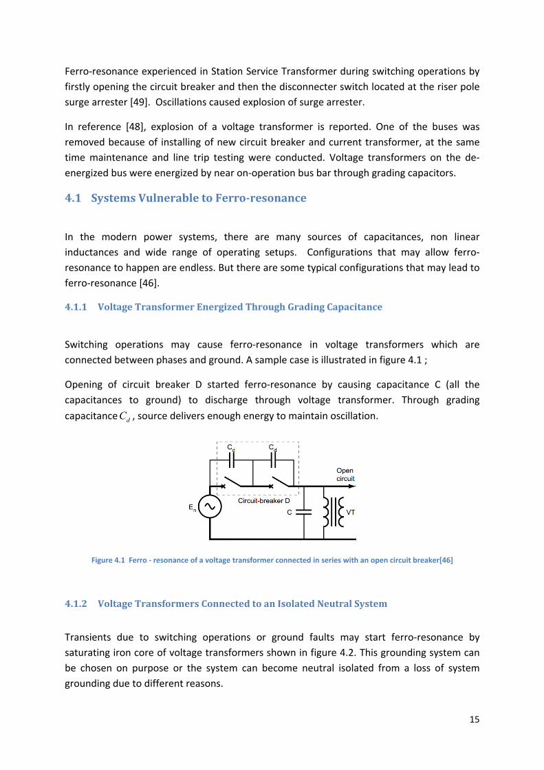
connected between phases and ground. A sample case is illustrated in figure 4.1 ;
Opening of circuit breaker D started ferro‐resonance by causing capacitance C (all the
capacitances to ground) to discharge through voltage transformer. Through grading
capacitance dC , source delivers enough energy to maintain oscillation.
Figure 4.1 Ferro ‐ resonance of a voltage transformer connected in series with an open circuit breaker[46]
4.1.2 VoltageTransformersConnectedtoanIsolatedNeutralSystem
Transients due to switching operations or ground faults may start ferro‐resonance by
saturating iron core of voltage transformers shown in figure 4.2. This grounding system can
be chosen on purpose or the system can become neutral isolated from a loss of system
grounding due to different reasons.
16
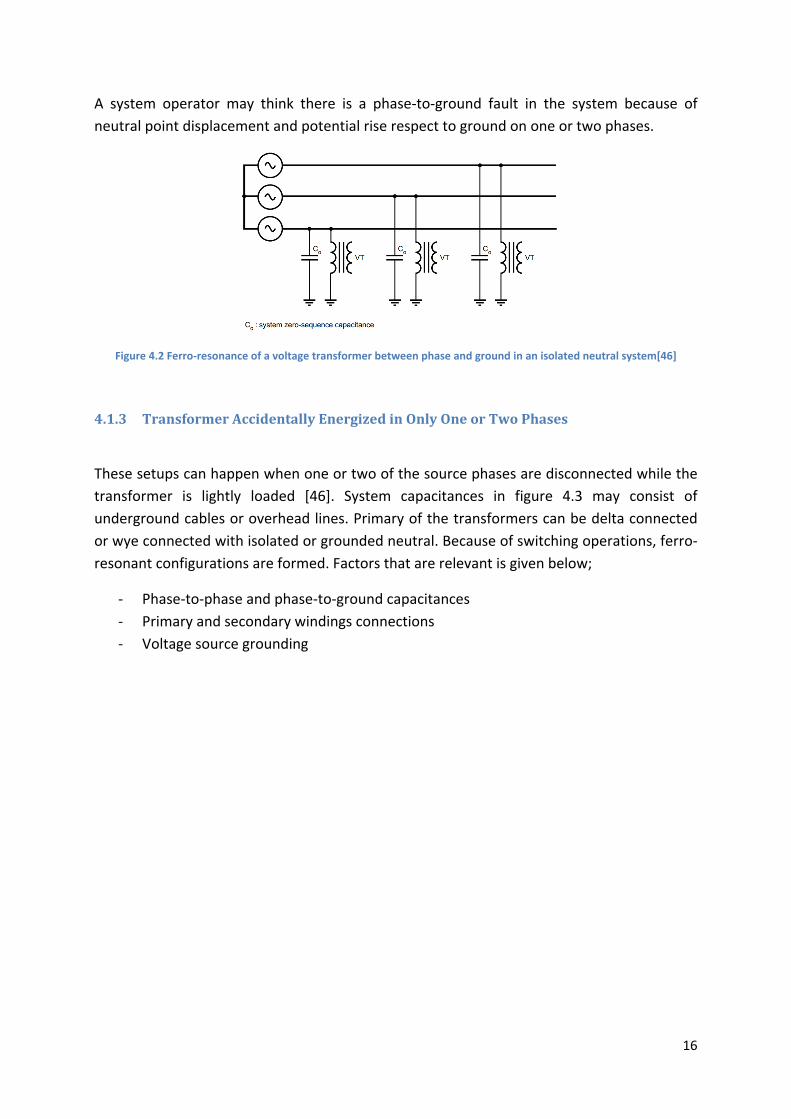
A system operator may think there is a phase‐to‐ground fault in the system because of
neutral point displacement and potential rise respect to ground on one or two phases.
Figure 4.2 Ferro‐resonance of a voltage transformer between phase and ground in an isolated neutral system[46]
4.1.3 TransformerAccidentallyEnergizedinOnlyOneorTwoPhases
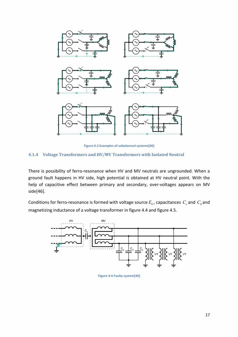
These setups can happen when one or two of the source phases are disconnected while the
transformer is lightly loaded [46]. System capacitances in figure 4.3 may consist of
underground cables or overhead lines. Primary of the transformers can be delta connected
or wye connected with isolated or grounded neutral. Because of switching operations, ferro‐
resonant configurations are formed. Factors that are relevant is given below;
‐ Phase‐to‐phase and phase‐to‐ground capacitances
‐ Primary and secondary windings connections
‐ Voltage source grounding
17
Figure 4.3 Examples of unbalanced systems[46]
4.1.4 VoltageTransformersandHV/MVTransformerswithIsolatedNeutral
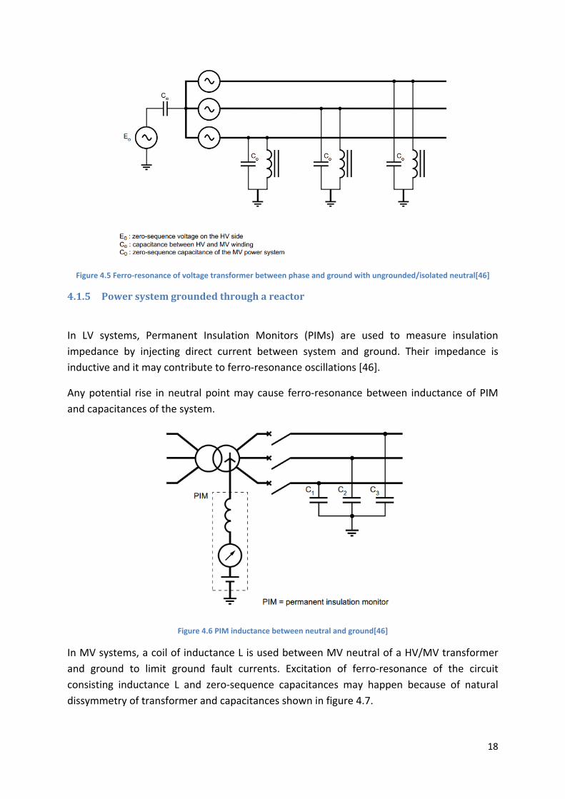
There is possibility of ferro‐resonance when HV and MV neutrals are ungrounded. When a
ground fault happens in HV side, high potential is obtained at HV neutral point. With the
help of capacitive effect between primary and secondary, over‐voltages appears on MV
side[46].
Conditions for ferro‐resonance is formed with voltage source 0E , capacitances eC and 0C and
magnetizing inductance of a voltage transformer in figure 4.4 and figure 4.5.
Figure 4.4 Faulty system[46]
18
Figure 4.5 Ferro‐resonance of voltage transformer between phase and ground with ungrounded/isolated neutral[46]
4.1.5 Powersystemgroundedthroughareactor
In LV systems, Permanent Insulation Monitors (PIMs) are used to measure insulation
impedance by injecting direct current between system and ground. Their impedance is
inductive and it may contribute to ferro‐resonance oscillations [46].
Any potential rise in neutral point may cause ferro‐resonance between inductance of PIM
and capacitances of the system.
Figure 4.6 PIM inductance between neutral and ground[46]
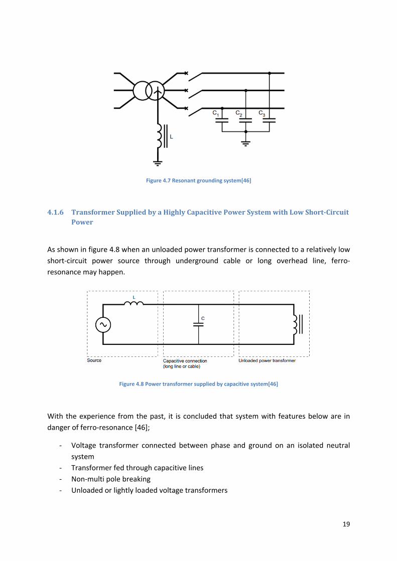
In MV systems, a coil of inductance L is used between MV neutral of a HV/MV transformer
and ground to limit ground fault currents. Excitation of ferro‐resonance of the circuit
consisting inductance L and zero‐sequence capacitances may happen because of natural
dissymmetry of transformer and capacitances shown in figure 4.7.
19
Figure 4.7 Resonant grounding system[46]
4.1.6 TransformerSuppliedbyaHighlyCapacitivePowerSystemwithLowShort‐CircuitPower
As shown in figure 4.8 when an unloaded power transformer is connected to a relatively low
short‐circuit power source through underground cable or long overhead line, ferro‐
resonance may happen.
Figure 4.8 Power transformer supplied by capacitive system[46]
With the experience from the past, it is concluded that system with features below are in
danger of ferro‐resonance [46];
‐ Voltage transformer connected between phase and ground on an isolated neutral
system
‐ Transformer fed through capacitive lines
‐ Non‐multi pole breaking
‐ Unloaded or lightly loaded voltage transformers
20
5 PreventingFerro‐resonance
Methods to prevent ferro‐resonance and its harmful effects are listed as follows;
‐ Avoiding configurations vulnerable to ferro‐resonance
‐ Ensuring system parameters are not causing risk of ferro‐resonance
‐ Ensuring energy supplied by the source is not enough to sustain oscillations (
introducing damping to the system )
International standards state that resonance over voltages should be prevented or limited,
those voltage values cannot be taken basis for insulation design. So in theory, current design
of insulations and surge arresters do not provide protection against ferro‐resonance [56].
There are some research on dynamical damping of ferro‐resonance, prototypes are
introduced [19], [20] but the most common used practice is static damping with damping
resistors.
For configurations in figure 4.3, following practical solutions are advised [46];
‐ Lowering capacitance between circuit breaker and transformer
‐ Avoiding use of transformers at 10% of its rated capacity
‐ Avoiding no‐load energizing
‐ Prohibiting single‐phase operations
In case of MV power systems grounded through a reactor figure 4.7, overcompensation of
power frequency capacitance component of the ground fault current can be done or a
resistive component to increase losses can also be added [46].
For power transformers whose are fed through capacitive lines, the best solution proposed
is avoiding risky situations when active power delivery is less than 10% of the transformer
rated power [46].
5.1 DampingFerro‐resonanceinVoltageTransformers
As mentioned before, voltage transformers connected between phase and ground in neutral
isolated systems is dangerous for ferro‐resonance oscillations to happen.
It is advised that avoid wye‐connections of voltage transformer primaries with grounded
neutral by leaving neutral of primaries ungrounded or using delta connection instead
[18],[40]. If wye‐connection for primaries is used, only way left to damp a possible oscillation
is to introduce load resistances.
21
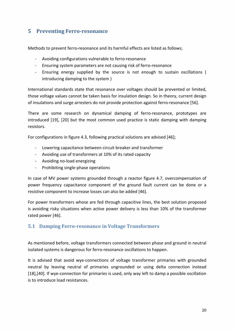
5.1.1 VoltageTransformerswithoneSecondaryWinding
Even though resistors will consume power during operation, damping resistors are used to
damp possible ferro‐resonant oscillations in figure 5.1.
Recommended minimum values of resistance R and power rating of resistor RP are
calculated with rated values of transformer in (5.1) and (5.2) [40], [46].
2
.s
t m
UR
k P P
(5.1)
2s
R
UP
R (5.2)
where;
sU : rated secondary voltage (V)
k : factor between 0.25 and 1 regarding errors and service conditions
tP : voltage transformer’s rated output (VA)
mP : power required for measurement (VA)
Figure 5.1 Damping for voltage transformer with one secondary[46]
22
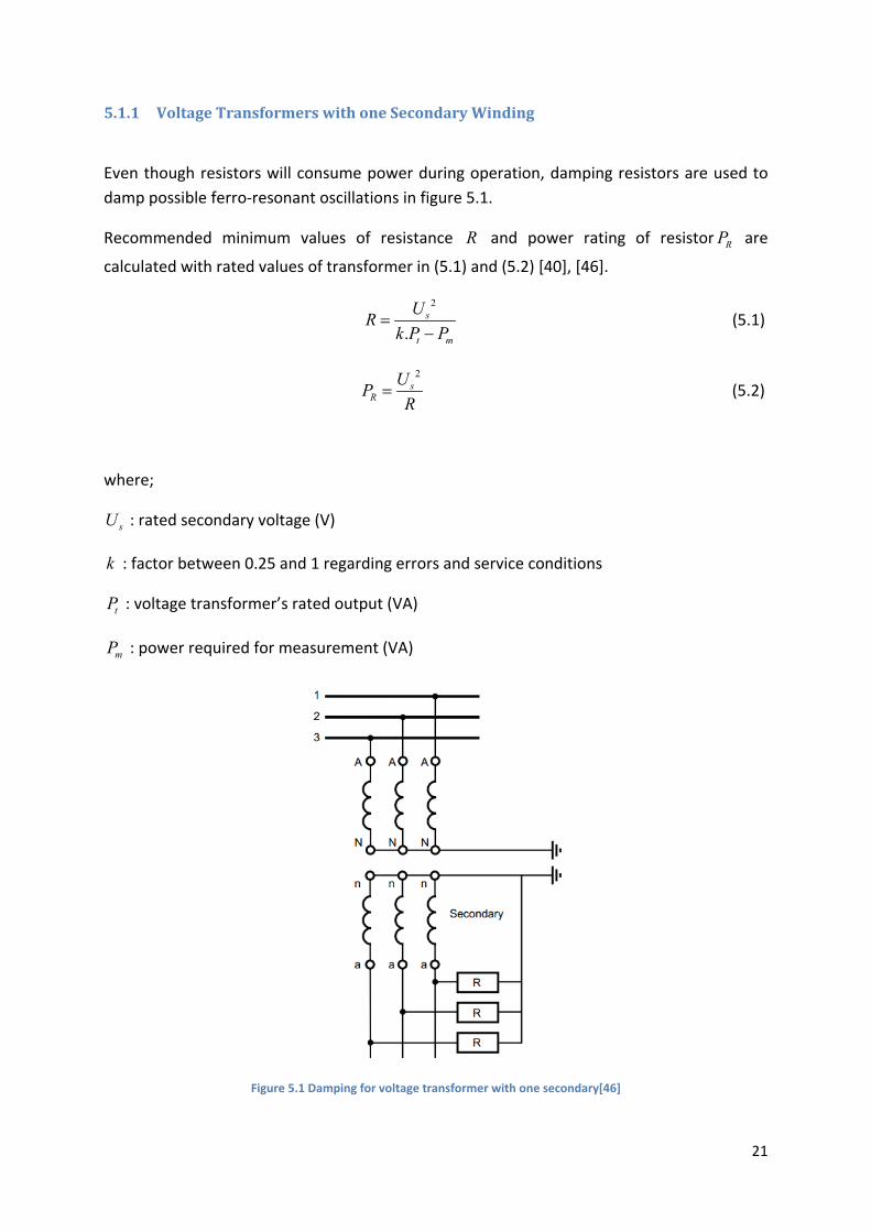
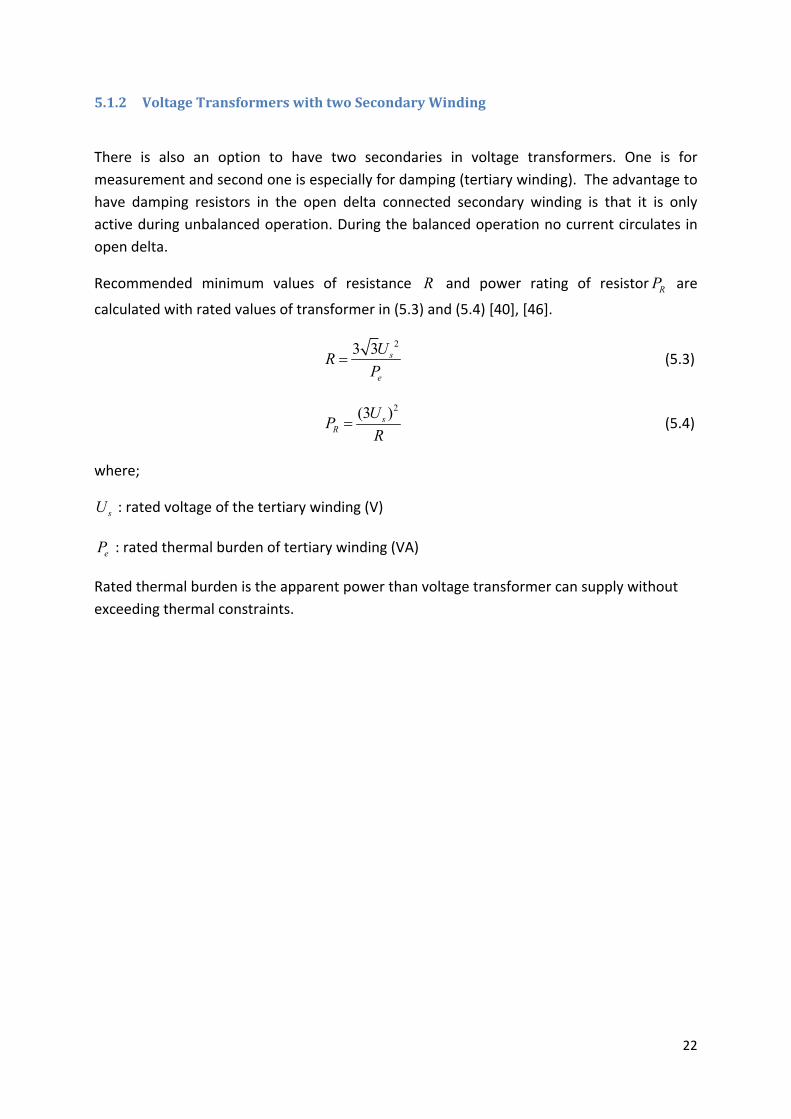
5.1.2 VoltageTransformerswithtwoSecondaryWinding
There is also an option to have two secondaries in voltage transformers. One is for
measurement and second one is especially for damping (tertiary winding). The advantage to
have damping resistors in the open delta connected secondary winding is that it is only
active during unbalanced operation. During the balanced operation no current circulates in
open delta.
Recommended minimum values of resistance R and power rating of resistor RP are
calculated with rated values of transformer in (5.3) and (5.4) [40], [46].
23 3 s
e
UR
P (5.3)
2(3 )sR
UP
R (5.4)
where;
sU : rated voltage of the tertiary winding (V)
eP : rated thermal burden of tertiary winding (VA)
Rated thermal burden is the apparent power than voltage transformer can supply without
exceeding thermal constraints.
23
Figure 5.2 Damping system for voltage transformer with two secondary[46]
6 ModelofNon‐linearity
The complexity of the whole ferro‐resonance problem is caused by non‐linear inductances in
the system. Relationship between flux and magnetizing current for voltage transformer
should be formed in order to study ferro‐resonance in time domain and also in frequency
domain.
In many studies (6.1) is taken model for saturation curve characteristics for voltage
transformers [12],[22],[27],[31],[33],[36],[37].
1 2n
mi k k (6.1)
where;
mi : Magnetizing current (p.u)
1k , 2k : Polynomial constants
: Core magnetic flux (p.u)
24
Polynomial constants 1k , 2k have impact on the linear and saturated regions of
magnetization characteristics. 1k is related to linear part of the saturation curve whereas 2k
is related to saturated zone when iron core is driven into saturation by high magnetizing
current.
The behavior of a given system is extremely sensitive to non‐linearity of the inductances so
for sake of accurate results polynomial constants and index n must be obtained with
precision. Shape of magnetizing curve and saturation knee position are important
characteristics of magnetizing curve of a voltage transformer. These curves can be created
with help of records from real measurements of inrush currents during energization of a
given voltage transformer.
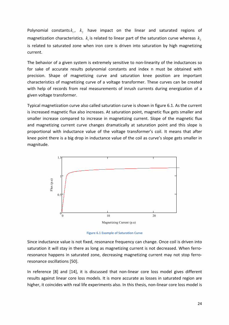
Typical magnetization curve also called saturation curve is shown in figure 6.1. As the current
is increased magnetic flux also increases. At saturation point, magnetic flux gets smaller and
smaller increase compared to increase in magnetizing current. Slope of the magnetic flux
and magnetizing current curve changes dramatically at saturation point and this slope is
proportional with inductance value of the voltage transformer’s coil. It means that after
knee point there is a big drop in inductance value of the coil as curve’s slope gets smaller in
magnitude.
Figure 6.1 Example of Saturation Curve
Since inductance value is not fixed, resonance frequency can change. Once coil is driven into
saturation it will stay in there as long as magnetizing current is not decreased. When ferro‐
resonance happens in saturated zone, decreasing magnetizing current may not stop ferro‐
resonance oscillations [50].
In reference [8] and [14], it is discussed that non‐linear core loss model gives different
results against linear core loss models. It is more accurate as losses in saturated region are
higher, it coincides with real life experiments also. In this thesis, non‐linear core loss model is
0 10 200
0.5
1
1.5
Magnetizing Current (p.u)
Flu
x (p
.u)
25
not used for sake of simplicity for the analysis. But it will be kept in mind that in ferro‐
resonance operation core losses are getting relatively higher.
7 Ferro‐resonanceinTime‐Domain
Time‐domain solutions of ferro‐resonant circuits do not give broad vision of these
phenomena but can give examples of different kind of ferro‐resonances. A sample
configuration leading to ferro‐resonance is examined.
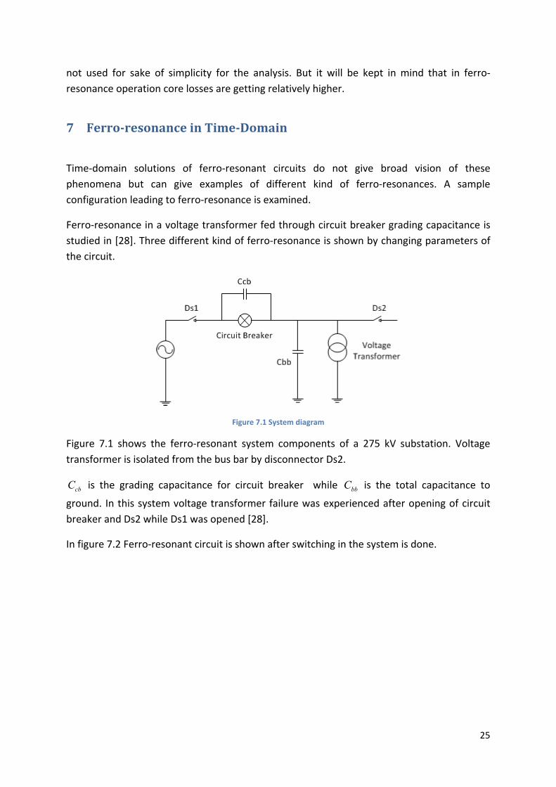
Ferro‐resonance in a voltage transformer fed through circuit breaker grading capacitance is
studied in [28]. Three different kind of ferro‐resonance is shown by changing parameters of
the circuit.
Figure 7.1 System diagram
Figure 7.1 shows the ferro‐resonant system components of a 275 kV substation. Voltage
transformer is isolated from the bus bar by disconnector Ds2.
cbC is the grading capacitance for circuit breaker while bbC is the total capacitance to
ground. In this system voltage transformer failure was experienced after opening of circuit
breaker and Ds2 while Ds1 was opened [28].
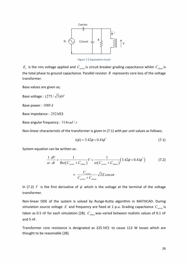
In figure 7.2 Ferro‐resonant circuit is shown after switching in the system is done.
26
Figure 7.2 Equivalent circuit
sE is the rms voltage applied and seriesC is circuit breaker grading capacitance whilst shuntC is
the total phase to ground capacitance. Parallel resistor R represents core loss of the voltage
transformer.
Base values are given as;
Base voltage : (275 / 3)kV
Base power : 100VA
Base impedance : 252M
Base angular frequency : 314 /rad s
Non‐linear characteristic of the transformer is given in (7.1) with per unit values as follows;
7( ) 3.42 0.41i (7.1)
System equation can be written as:
71 1 13.42 0.41
series shunt series shunt
dVV
dt R C C C C
(7.2)
= 2 cosseries
series shunt
CE t
C C
In (7.2) V is the first derivative of which is the voltage at the terminal of the voltage
transformer.
Non‐linear ODE of the system is solved by Runge‐Kutta algorithm in MATHCAD. During
simulation source voltage E and frequency are fixed at 1 p.u. Grading capacitance seriesC is
taken as 0.5 nF for each simulation [28]. shuntC was varied between realistic values of 0.1 nF
and 5 nF.
Transformer core resistance is designated as 225M to cause 112 W losses which are
thought to be reasonable [28].
27
Initial values for flux and flux first derivative are selected as ( ) 2V t p.u and ( ) 0t at
0t . This means that circuit breaker operation is at maximum voltage.
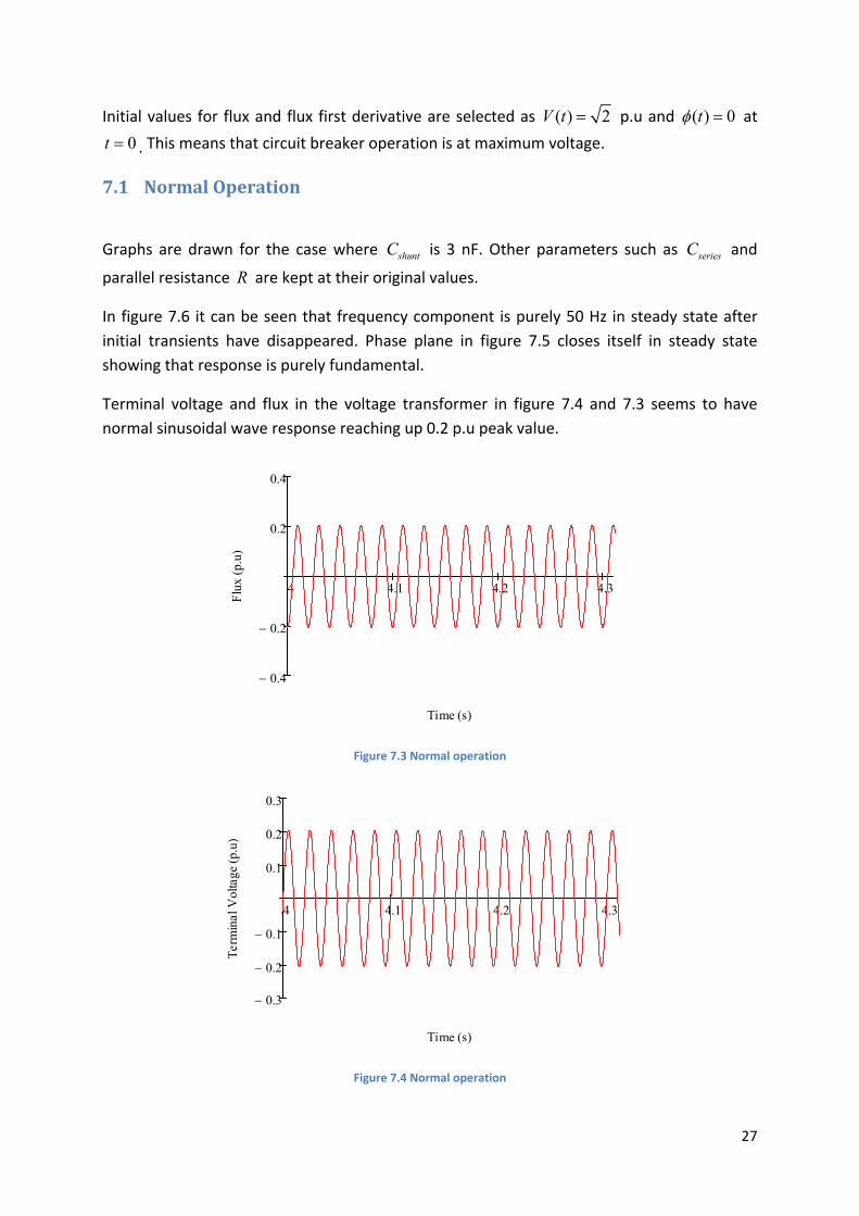
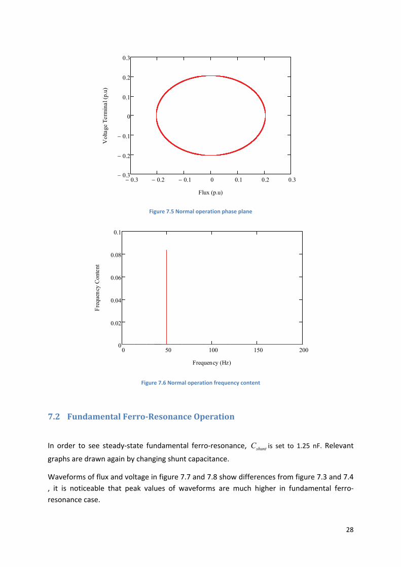
7.1 NormalOperation
Graphs are drawn for the case where shuntC is 3 nF. Other parameters such as seriesC and
parallel resistance R are kept at their original values.
In figure 7.6 it can be seen that frequency component is purely 50 Hz in steady state after
initial transients have disappeared. Phase plane in figure 7.5 closes itself in steady state
showing that response is purely fundamental.
Terminal voltage and flux in the voltage transformer in figure 7.4 and 7.3 seems to have
normal sinusoidal wave response reaching up 0.2 p.u peak value.
Figure 7.3 Normal operation
Figure 7.4 Normal operation
4 4.1 4.2 4.3
0.4
0.2
0.2
0.4
Time (s)
Flu
x (p
.u)
4 4.1 4.2 4.3
0.3
0.2
0.1
0.1
0.2
0.3
Time (s)
Ter
min
al V
olta
ge (
p.u)
28
Figure 7.5 Normal operation phase plane
Figure 7.6 Normal operation frequency content
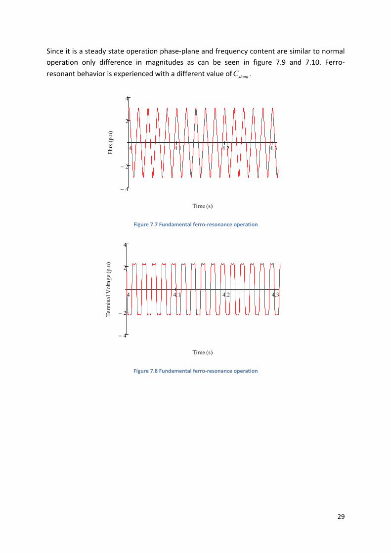
7.2 FundamentalFerro‐ResonanceOperation
In order to see steady‐state fundamental ferro‐resonance, shuntC is set to 1.25 nF. Relevant
graphs are drawn again by changing shunt capacitance.
Waveforms of flux and voltage in figure 7.7 and 7.8 show differences from figure 7.3 and 7.4
, it is noticeable that peak values of waveforms are much higher in fundamental ferro‐
resonance case.
0.3 0.2 0.1 0 0.1 0.2 0.30.3
0.2
0.1
0
0.1
0.2
0.3
Flux (p.u)
Vol
tage
Ter
min
al (
p.u)
0 50 100 150 2000
0.02
0.04
0.06
0.08
0.1
Frequency (Hz)
Fre
quen
cy C
onte
nt
29
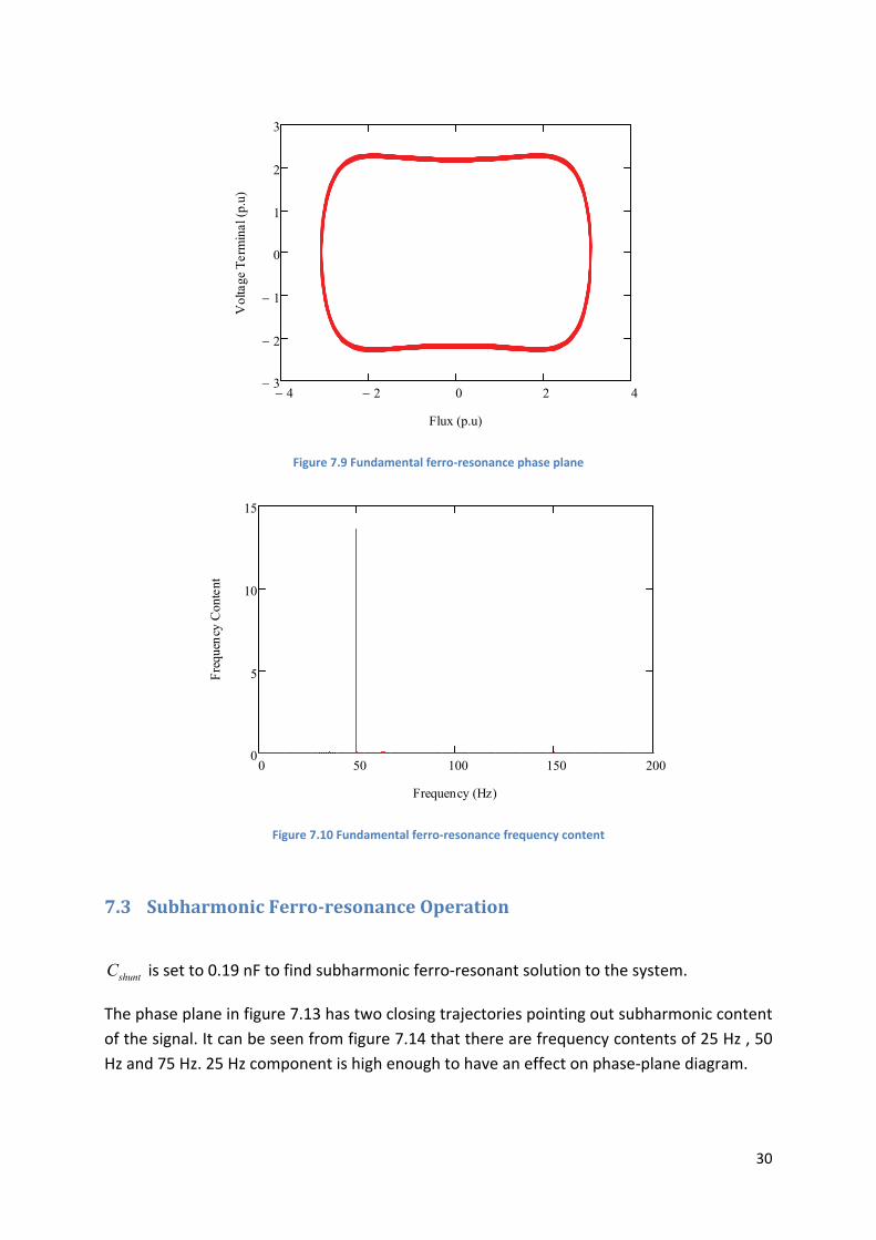
Since it is a steady state operation phase‐plane and frequency content are similar to normal
operation only difference in magnitudes as can be seen in figure 7.9 and 7.10. Ferro‐
resonant behavior is experienced with a different value of shuntC .
Figure 7.7 Fundamental ferro‐resonance operation
Figure 7.8 Fundamental ferro‐resonance operation
4 4.1 4.2 4.3
4
2
2
4
Time (s)
Flu
x (p
.u)
4 4.1 4.2 4.3
4
2
2
4
Time (s)
Ter
min
al V
olta
ge (
p.u)
30
Figure 7.9 Fundamental ferro‐resonance phase plane
Figure 7.10 Fundamental ferro‐resonance frequency content
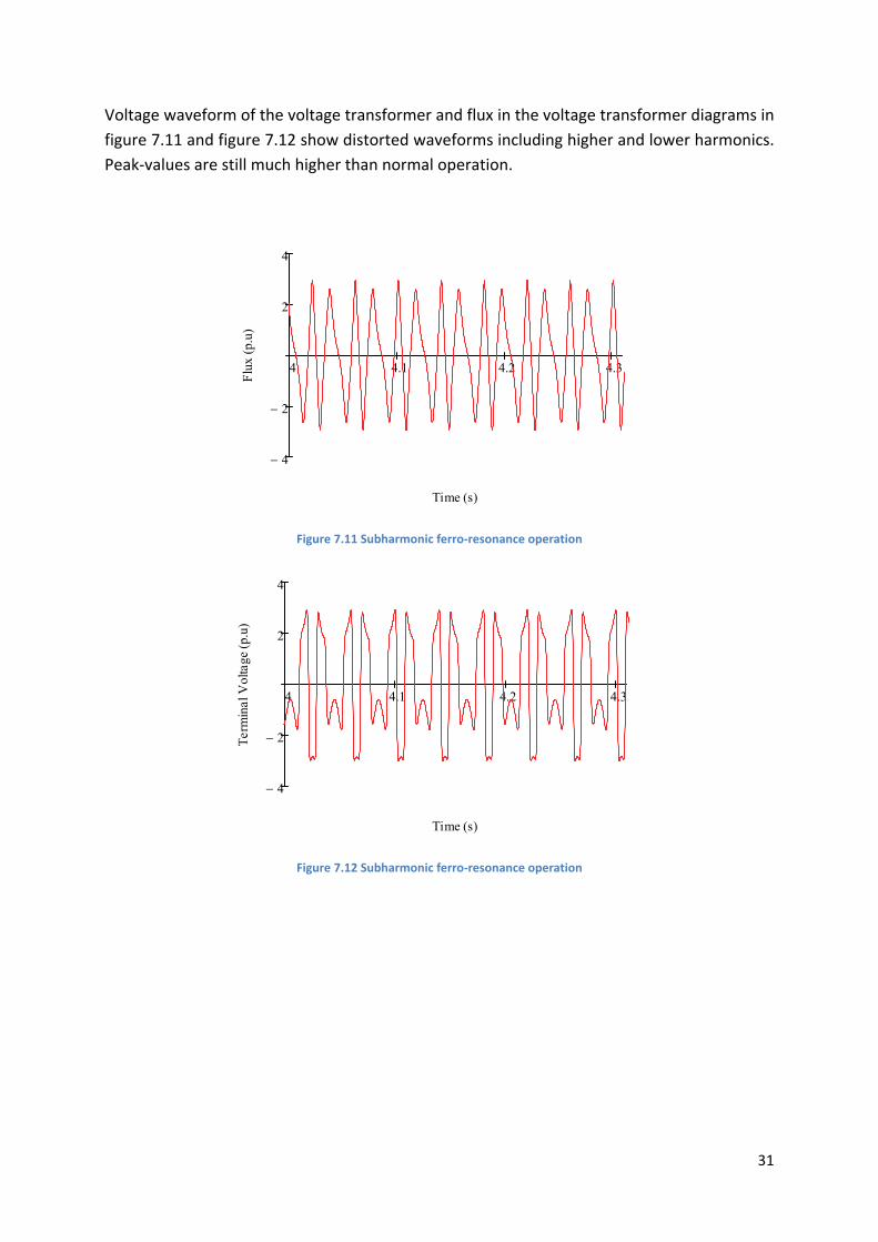
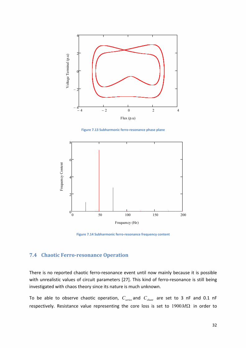
7.3 SubharmonicFerro‐resonanceOperation
shuntC is set to 0.19 nF to find subharmonic ferro‐resonant solution to the system.
The phase plane in figure 7.13 has two closing trajectories pointing out subharmonic content
of the signal. It can be seen from figure 7.14 that there are frequency contents of 25 Hz , 50
Hz and 75 Hz. 25 Hz component is high enough to have an effect on phase‐plane diagram.
4 2 0 2 43
2
1
0
1
2
3
Flux (p.u)
Vol
tage
Ter
min
al (
p.u)
0 50 100 150 2000
5
10
15
Frequency (Hz)
Fre
quen
cy C
onte
nt
31
Voltage waveform of the voltage transformer and flux in the voltage transformer diagrams in
figure 7.11 and figure 7.12 show distorted waveforms including higher and lower harmonics.
Peak‐values are still much higher than normal operation.
Figure 7.11 Subharmonic ferro‐resonance operation
Figure 7.12 Subharmonic ferro‐resonance operation
4 4.1 4.2 4.3
4
2
2
4
Time (s)
Flu
x (p
.u)
4 4.1 4.2 4.3
4
2
2
4
Time (s)
Ter
min
al V
olta
ge (
p.u)
32
Figure 7.13 Subharmonic ferro‐resonance phase plane
Figure 7.14 Subharmonic ferro‐resonance frequency content
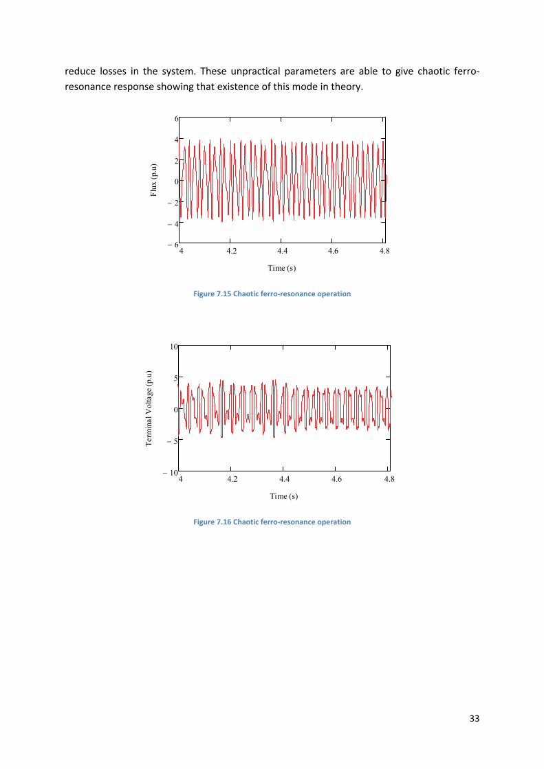
7.4 ChaoticFerro‐resonanceOperation
There is no reported chaotic ferro‐resonance event until now mainly because it is possible
with unrealistic values of circuit parameters [27]. This kind of ferro‐resonance is still being
investigated with chaos theory since its nature is much unknown.
To be able to observe chaotic operation, seriesC and shuntC are set to 3 nF and 0.1 nF
respectively. Resistance value representing the core loss is set to 1900M in order to
4 2 0 2 44
2
0
2
4
Flux (p.u)
Vol
tage
Ter
min
al (
p.u)
0 50 100 150 2000
2
4
6
8
Frequency (Hz)
Fre
quen
cy C
onte
nt
33
reduce losses in the system. These unpractical parameters are able to give chaotic ferro‐
resonance response showing that existence of this mode in theory.
Figure 7.15 Chaotic ferro‐resonance operation
Figure 7.16 Chaotic ferro‐resonance operation
4 4.2 4.4 4.6 4.86
4
2
0
2
4
6
Time (s)
Flu
x (p
.u)
4 4.2 4.4 4.6 4.810
5
0
5
10
Time (s)
Ter
min
al V
olta
ge (
p.u)
34
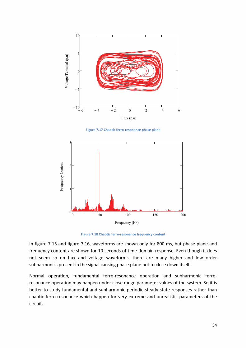
Figure 7.17 Chaotic ferro‐resonance phase plane
Figure 7.18 Chaotic ferro‐resonance frequency content
In figure 7.15 and figure 7.16, waveforms are shown only for 800 ms, but phase plane and
frequency content are shown for 10 seconds of time‐domain response. Even though it does
not seem so on flux and voltage waveforms, there are many higher and low order
subharmonics present in the signal causing phase plane not to close down itself.
Normal operation, fundamental ferro‐resonance operation and subharmonic ferro‐
resonance operation may happen under close range parameter values of the system. So it is
better to study fundamental and subharmonic periodic steady state responses rather than
chaotic ferro‐resonance which happen for very extreme and unrealistic parameters of the
circuit.
6 4 2 0 2 4 610
5
0
5
10
Flux (p.u)
Vol
tage
Ter
min
al (
p.u)
0 50 100 150 2000
1
2
3
Frequency (Hz)
Fre
quen
cy C
onte
nt
35
Time‐domain analyses give narrow vision to understand the risk of ferro‐resonance. In
literature, it is found that differentiating the initial values to the ODE solver might give
different results for same parameters of the system [8], [12], [27]. Since there are so many
initial and parameter values that can be used, it is unrealistic to try out every single scenario.
In reference [12], it is shown that a small increment on parameters can lead to different
operation modes.
8 AnalyticalHarmonicBalanceMethod
Harmonic balance is a method for the study of non‐linear oscillating systems which are
defined by non‐linear ordinary differential equations. The basis of the method is to
substitute unknown in the system by assumed solution so that approximate periodic
solutions of non‐linear ordinary differential equations can be found. The assumed solution
can be defined as a sum of steady state sinusoids (Fourier series) that includes the forcing
frequency in addition to any significant harmonics.
Theory of harmonic balance method is explained in [51], [52], [53]. Practice of this theory on
ferro‐resonant circuits is done in [31], [32], [33].
An example of application of harmonic balance method will be given to show approach to
fundamental ferro‐resonant behavior.
8.1 ApplicationofHarmonicBalanceonExampleSystem
In figure 4.3, there are cases shown where ferro‐resonance configuration is formed when
one or two of the source phases are lost while the transformer is lightly loaded. This may be
caused by single phase switching operations such as clearing of single phase fusing and
single phase reclosing.
In the following case, one phase of the system was open while other two are closed. This
leads to an induced voltage in the open phase because of capacitances in the system [11].
36
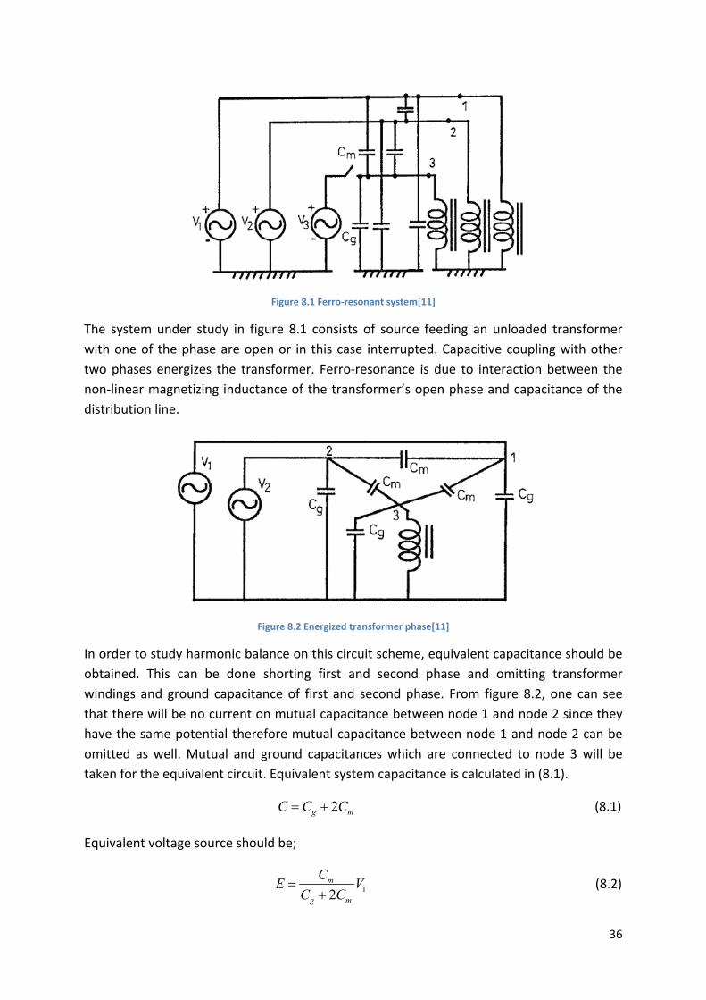
Figure 8.1 Ferro‐resonant system[11]
The system under study in figure 8.1 consists of source feeding an unloaded transformer
with one of the phase are open or in this case interrupted. Capacitive coupling with other
two phases energizes the transformer. Ferro‐resonance is due to interaction between the
non‐linear magnetizing inductance of the transformer’s open phase and capacitance of the
distribution line.
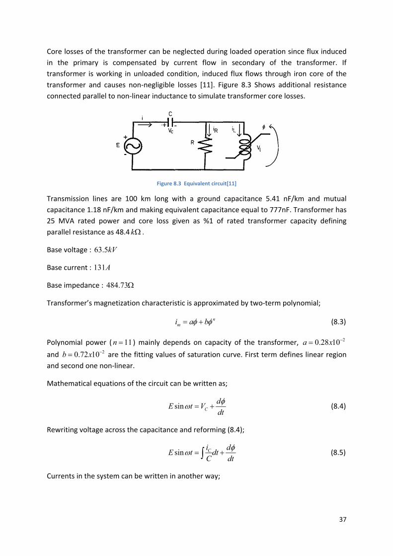
Figure 8.2 Energized transformer phase[11]
In order to study harmonic balance on this circuit scheme, equivalent capacitance should be
obtained. This can be done shorting first and second phase and omitting transformer
windings and ground capacitance of first and second phase. From figure 8.2, one can see
that there will be no current on mutual capacitance between node 1 and node 2 since they
have the same potential therefore mutual capacitance between node 1 and node 2 can be
omitted as well. Mutual and ground capacitances which are connected to node 3 will be
taken for the equivalent circuit. Equivalent system capacitance is calculated in (8.1).
2g mC C C (8.1)
Equivalent voltage source should be;
12m
g m
CE V
C C
(8.2)
37
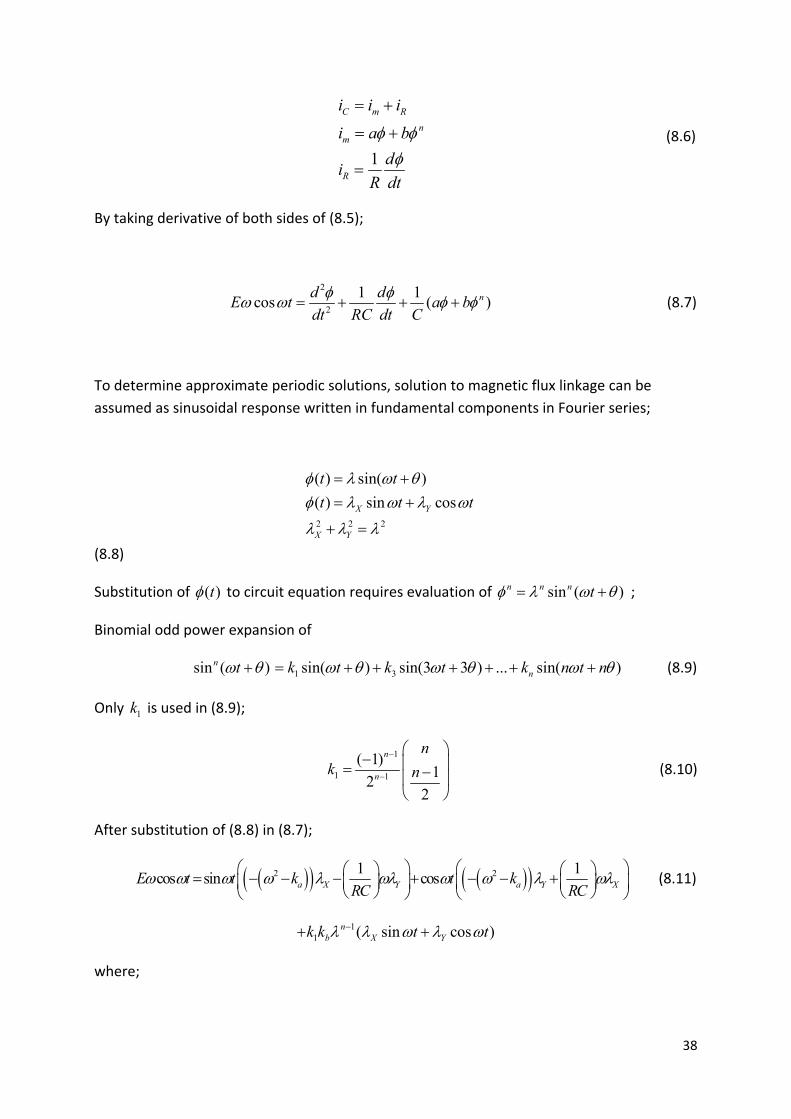
Core losses of the transformer can be neglected during loaded operation since flux induced
in the primary is compensated by current flow in secondary of the transformer. If
transformer is working in unloaded condition, induced flux flows through iron core of the
transformer and causes non‐negligible losses [11]. Figure 8.3 Shows additional resistance
connected parallel to non‐linear inductance to simulate transformer core losses.
Figure 8.3 Equivalent circuit[11]
Transmission lines are 100 km long with a ground capacitance 5.41 nF/km and mutual
capacitance 1.18 nF/km and making equivalent capacitance equal to 777nF. Transformer has
25 MVA rated power and core loss given as %1 of rated transformer capacity defining
parallel resistance as 48.4 k .
Base voltage : 63.5kV
Base current : 131A
Base impedance : 484.73
Transformer’s magnetization characteristic is approximated by two‐term polynomial;
nmi a b (8.3)
Polynomial power ( 11n ) mainly depends on capacity of the transformer, 20.28 10a x
and 20.72 10b x are the fitting values of saturation curve. First term defines linear region
and second one non‐linear.
Mathematical equations of the circuit can be written as;
sin C
dE t V
dt
(8.4)
Rewriting voltage across the capacitance and reforming (8.4);
sin Ci dE t dt
C dt
(8.5)
Currents in the system can be written in another way;
38
1
C m R
nm
R
i i i
i a b
di
R dt
(8.6)
By taking derivative of both sides of (8.5);
2
2
1 1cos ( )n
d dE t a b
dt RC dt C
(8.7)
To determine approximate periodic solutions, solution to magnetic flux linkage can be
assumed as sinusoidal response written in fundamental components in Fourier series;
2 2 2
( ) sin( )
( ) sin cosX Y
X Y
t t
t t t
(8.8)
Substitution of ( )t to circuit equation requires evaluation of sin ( )n n n t ;
Binomial odd power expansion of
sin ( )n t 1 3sin( ) sin(3 3 ) ... sin( )nk t k t k n t n (8.9)
Only 1k is used in (8.9);
1
1 1
( 1)1
22
n
n
nk n
(8.10)
After substitution of (8.8) in (8.7);
2 21 1
cos sin cosa X Y a Y XE t t k t kRC RC
(8.11)
11 ( sin cos )nb X Yk k t t
where;
39
a
ak
C b
bk
C (8.12)
Equating sine and cosine terms in (8.11) makes the system dependent on the frequency and
circuit parameters;
2 11
2 11
( ) 0
( )
na b X Y
na b Y X
k k kRC
k k k ERC
(8.13)
2 2 2X Y
Equation (8.13) can be seen as;
' ' 0
' '
a x b y
a y a x H
(8.14)
After taking square and adding elements of (8.4);
2 2 2 2 2 2 2
2 2 2 2 2
' ( ) ' ( )
X Y
a x y b x y H
x y
(8.15)
Finally a form of polynomial is found from (8.15);
( 1)/22 1 0 0n np p p (8.16)
where;
22
0 2
1 b
p Ek k
222
1 2
1
a
b
kRC
pk k
(8.17)
2
21
2 a
b
kp
k k
Logic is to find the roots of (8.16) for each given source voltage peak value ; as expected for
some values of source voltage there were more than one positive real solution. By increasing
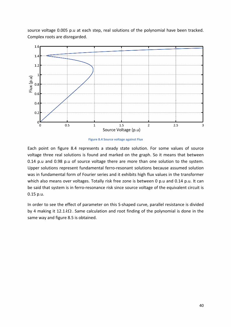
40
source voltage 0.005 p.u at each step, real solutions of the polynomial have been tracked.
Complex roots are disregarded.
Figure 8.4 Source voltage against Flux
Each point on figure 8.4 represents a steady state solution. For some values of source
voltage three real solutions is found and marked on the graph. So it means that between
0.14 p.u and 0.98 p.u of source voltage there are more than one solution to the system.
Upper solutions represent fundamental ferro‐resonant solutions because assumed solution
was in fundamental form of Fourier series and it exhibits high flux values in the transformer
which also means over voltages. Totally risk free zone is between 0 p.u and 0.14 p.u. It can
be said that system is in ferro‐resonance risk since source voltage of the equivalent circuit is
0.15 p.u.
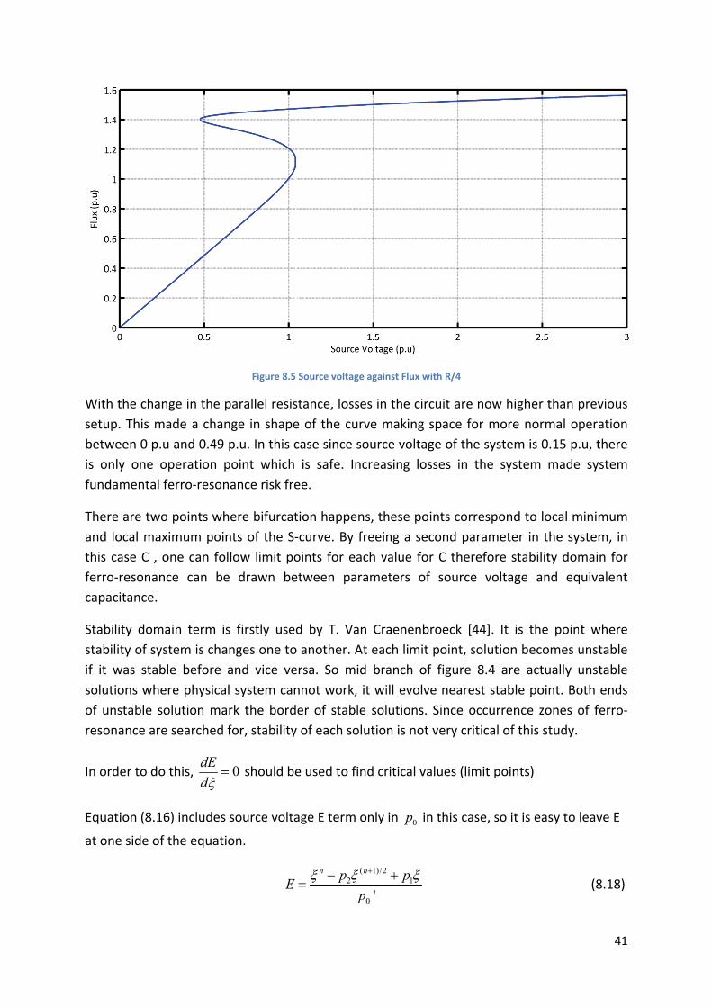
In order to see the effect of parameter on this S‐shaped curve, parallel resistance is divided
by 4 making it 12.1 k . Same calculation and root finding of the polynomial is done in the
same way and figure 8.5 is obtained.
With th
setup. T
betwee
is only
fundam
There a
and loc
this cas
ferro‐re
capacita
Stability
stability
if it wa
solution
of unsta
resonan
In order
Equatio
at one s
e change in
This made a
n 0 p.u and
one opera
mental ferro‐
re two poin
al maximum
se C , one c
esonance c
ance.
y domain t
y of system
s stable be
ns where ph
able solutio
nce are sear
r to do this,
on (8.16) inc
side of the e
Fi
n the parall
a change in
d 0.49 p.u. I
tion point
‐resonance
nts where b
m points of
can follow l
an be dra
erm is first
is changes
efore and v
hysical syst
on mark th
rched for, st
0dE
d sh
cludes sourc
equation.
igure 8.5 Sourc
el resistanc
n shape of t
n this case
which is s
risk free.
bifurcation h
f the S‐curv
imit points
wn betwee
tly used by
one to ano
vice versa.
em cannot
e border o
tability of e
ould be use
ce voltage E
n
E
ce voltage again
ce, losses in
the curve m
since sourc
afe. Increa
happens, th
ve. By freei
for each v
en parame
y T. Van Cr
other. At eac
So mid bra
work, it wi
f stable sol
each solutio
ed to find cr
E term only
( 1)/22
0 '
n np
p
nst Flux with R
the circuit
making spac
ce voltage o
sing losses
hese points
ng a second
value for C
eters of so
aenenbroec
ch limit poi
anch of fig
ill evolve ne
lutions. Sin
n is not ver
ritical value
in 0p in thi
21p
R/4
are now hi
ce for more
of the system
in the sys
correspond
d paramete
therefore s
ource voltag
ck [44]. It
nt, solution
gure 8.4 are
earest stab
ce occurren
ry critical of
s (limit poin
is case, so it
igher than p
e normal op
m is 0.15 p.
stem made
d to local m
er in the sy
stability dom
ge and eq
is the poin
n becomes u
e actually u
le point. Bo
nce zones o
this study.
nts)
t is easy to
41
previous
peration
.u, there
e system
minimum
ystem, in
main for
quivalent
t where
unstable
unstable
oth ends
of ferro‐
leave E
(8.18)
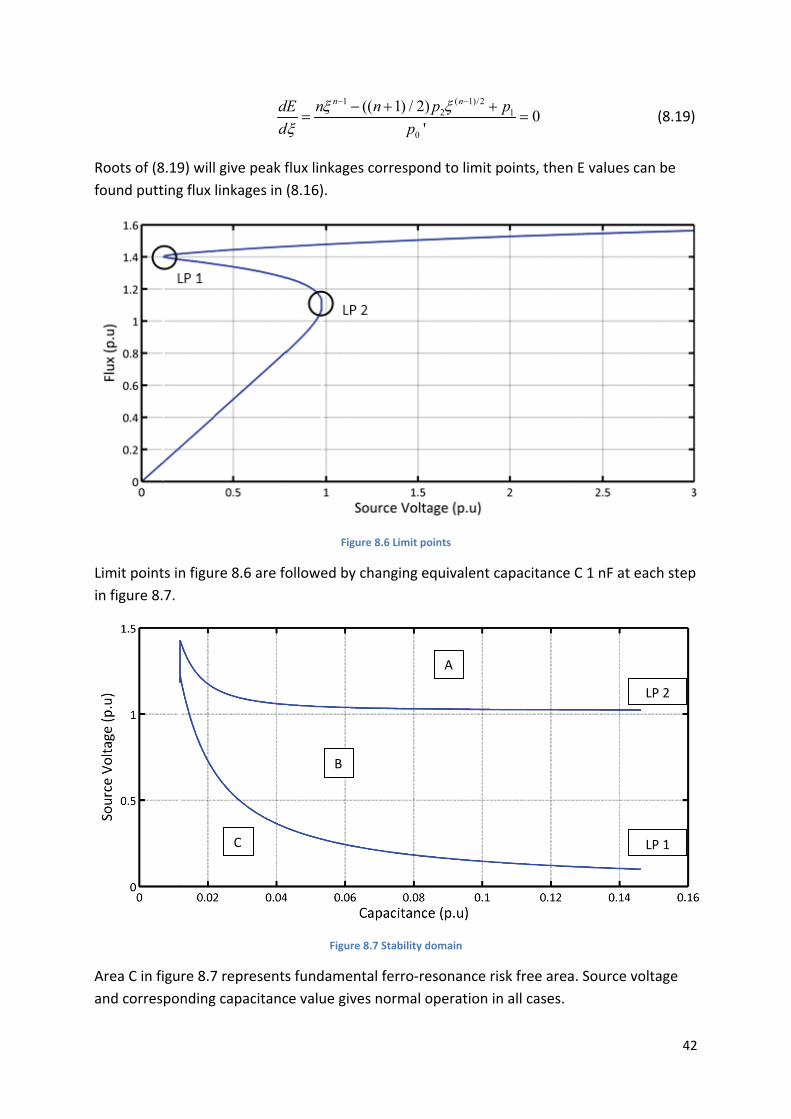
Roots o
found p
Limit po
in figure
Area C i
and cor
f (8.19) will
putting flux
oints in figu
e 8.7.
in figure 8.7
responding
dE
d
l give peak f
linkages in
re 8.6 are fo
7 represents
g capacitanc
C
1nndE
d
flux linkage
(8.16).
Figu
ollowed by
Figure
s fundamen
ce value giv
B
0
(( 1) / 2)
'
n
p
s correspon
ure 8.6 Limit po
changing e
e 8.7 Stability d
ntal ferro‐re
es normal o
( 1)/22) np
nd to limit p
oints
quivalent c
domain
esonance ris
operation in
A
1 0p
points, then
apacitance
sk free area
n all cases.
n E values ca
C 1 nF at ea
a. Source vo
42
(8.19)
an be
ach step
oltage
LP 2
LP 1
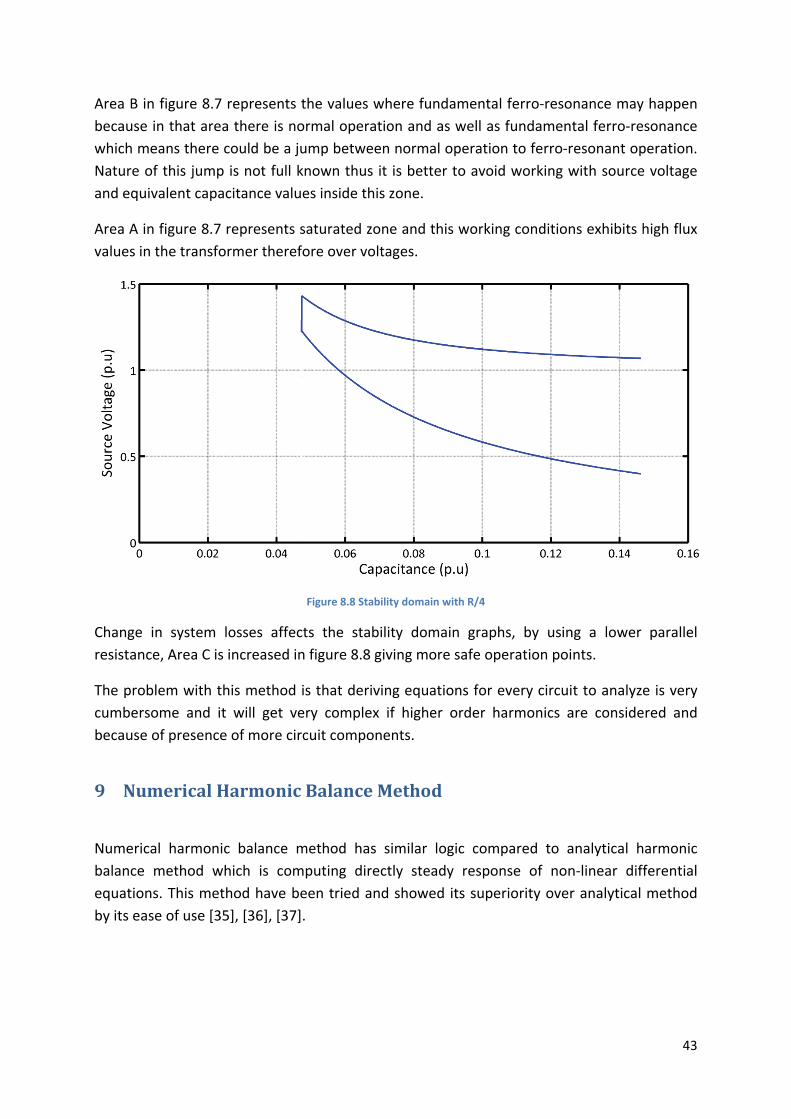
Area B
because
which m
Nature
and equ
Area A
values i
Change
resistan
The pro
cumber
because
9 Nu
Numeri
balance
equatio
by its ea
in figure 8.
e in that are
means there
of this jum
uivalent cap
in figure 8.7
n the transf
in system
nce, Area C
oblem with
rsome and
e of presenc
umerical
cal harmon
e method w
ons. This me
ase of use [
7 represent
ea there is
e could be a
mp is not ful
pacitance va
7 represent
former ther
m losses aff
is increased
this metho
it will get
ce of more
Harmon
nic balance
which is co
ethod have
35], [36], [3
ts the value
normal ope
a jump betw
ll known th
alues inside
ts saturated
refore over
Figure 8.8
fects the s
d in figure 8
od is that de
very comp
circuit com
nicBalanc
e method h
omputing d
been tried
37].
es where fu
eration and
ween norm
hus it is bett
this zone.
d zone and
voltages.
Stability doma
tability dom
8.8 giving m
eriving equ
plex if high
ponents.
ceMetho
has similar
directly ste
d and show
undamental
d as well as
al operatio
ter to avoid
this workin
ain with R/4
main graph
ore safe op
ations for e
er order h
od
logic com
eady respon
ed its supe
l ferro‐reso
fundament
n to ferro‐r
d working w
ng condition
hs, by usin
eration poi
every circui
armonics a
pared to a
nse of non
riority over
nance may
tal ferro‐re
resonant op
with source
ns exhibits h
ng a lower
nts.
t to analyze
are conside
analytical h
n‐linear diff
r analytical
43
y happen
sonance
peration.
e voltage
high flux
parallel
e is very
ered and
armonic
ferential
method
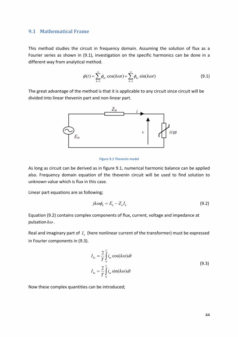
44
9.1 MathematicalFrame
This method studies the circuit in frequency domain. Assuming the solution of flux as a
Fourier series as shown in (9.1), investigation on the specific harmonics can be done in a
different way from analytical method.
1 1
( ) cos( ) sin( )n n
kc ksk k
t k t k t
(9.1)
The great advantage of the method is that it is applicable to any circuit since circuit will be
divided into linear thevenin part and non‐linear part.
Figure 9.1 Thevenin model
As long as circuit can be derived as in figure 9.1, numerical harmonic balance can be applied
also. Frequency domain equation of the thevenin circuit will be used to find solution to
unknown value which is flux in this case.
Linear part equations are as following;
k k k kjk E Z I (9.2)
Equation (9.2) contains complex components of flux, current, voltage and impedance at
pulsation k .
Real and imaginary part of kI (here nonlinear current of the transformer) must be expressed
in Fourier components in (9.3).
0
0
2cos( )
2sin( )
T
kc m
T
ks m
I i k dtT
I i k dtT
(9.3)
Now these complex quantities can be introduced;
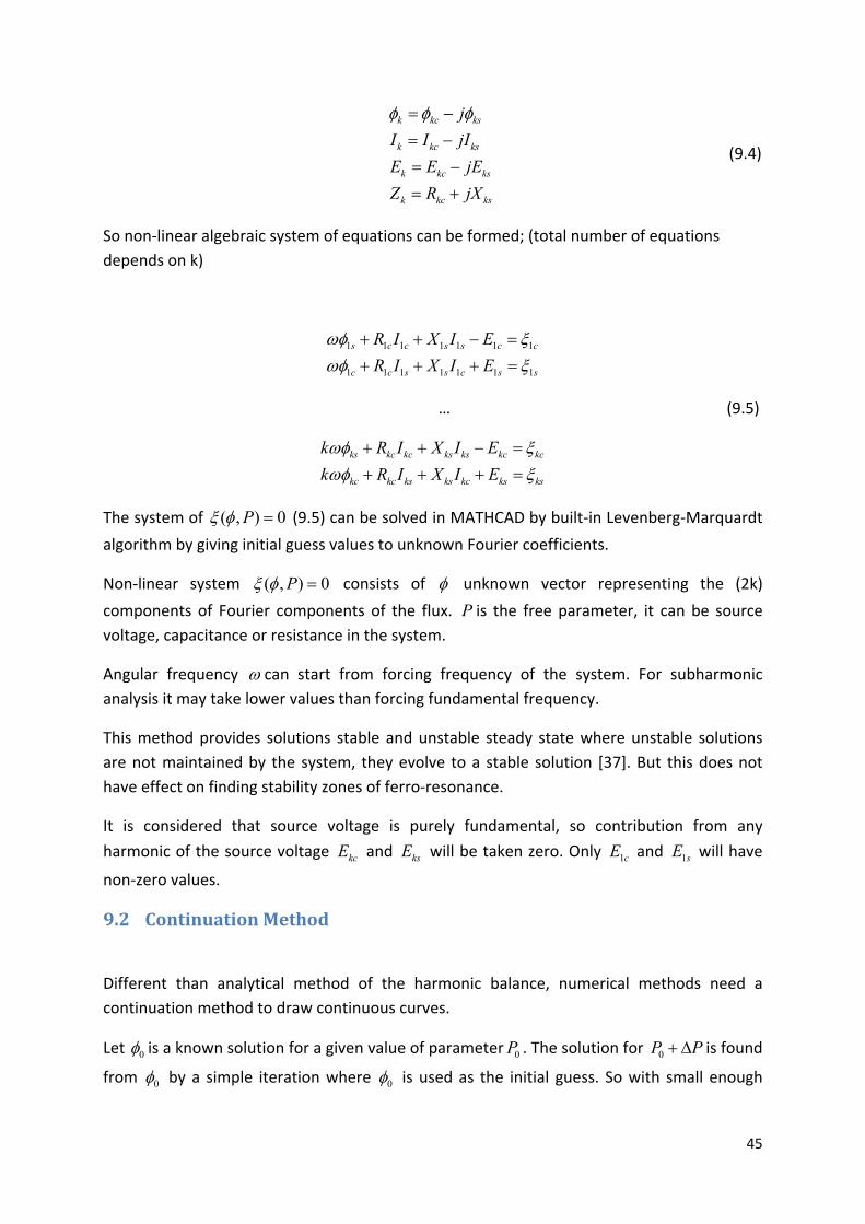
45
k kc ks
k kc ks
k kc ks
k kc ks
j
I I jI
E E jE
Z R jX
(9.4)
So non‐linear algebraic system of equations can be formed; (total number of equations
depends on k)
1 1 1 1 1 1 1
1 1 1 1 1 1 1
s c c s s c c
c c s s c s s
R I X I E
R I X I E
… (9.5)
ks kc kc ks ks kc kc
kc kc ks ks kc ks ks
k R I X I E
k R I X I E
The system of ( , ) 0P (9.5) can be solved in MATHCAD by built‐in Levenberg‐Marquardt
algorithm by giving initial guess values to unknown Fourier coefficients.
Non‐linear system ( , ) 0P consists of unknown vector representing the (2k)
components of Fourier components of the flux. P is the free parameter, it can be source
voltage, capacitance or resistance in the system.
Angular frequency can start from forcing frequency of the system. For subharmonic
analysis it may take lower values than forcing fundamental frequency.
This method provides solutions stable and unstable steady state where unstable solutions
are not maintained by the system, they evolve to a stable solution [37]. But this does not
have effect on finding stability zones of ferro‐resonance.
It is considered that source voltage is purely fundamental, so contribution from any
harmonic of the source voltage kcE and ksE will be taken zero. Only 1cE and 1sE will have
non‐zero values.
9.2 ContinuationMethod
Different than analytical method of the harmonic balance, numerical methods need a
continuation method to draw continuous curves.
Let 0 is a known solution for a given value of parameter 0P . The solution for 0P P is found
from 0 by a simple iteration where 0 is used as the initial guess. So with small enough
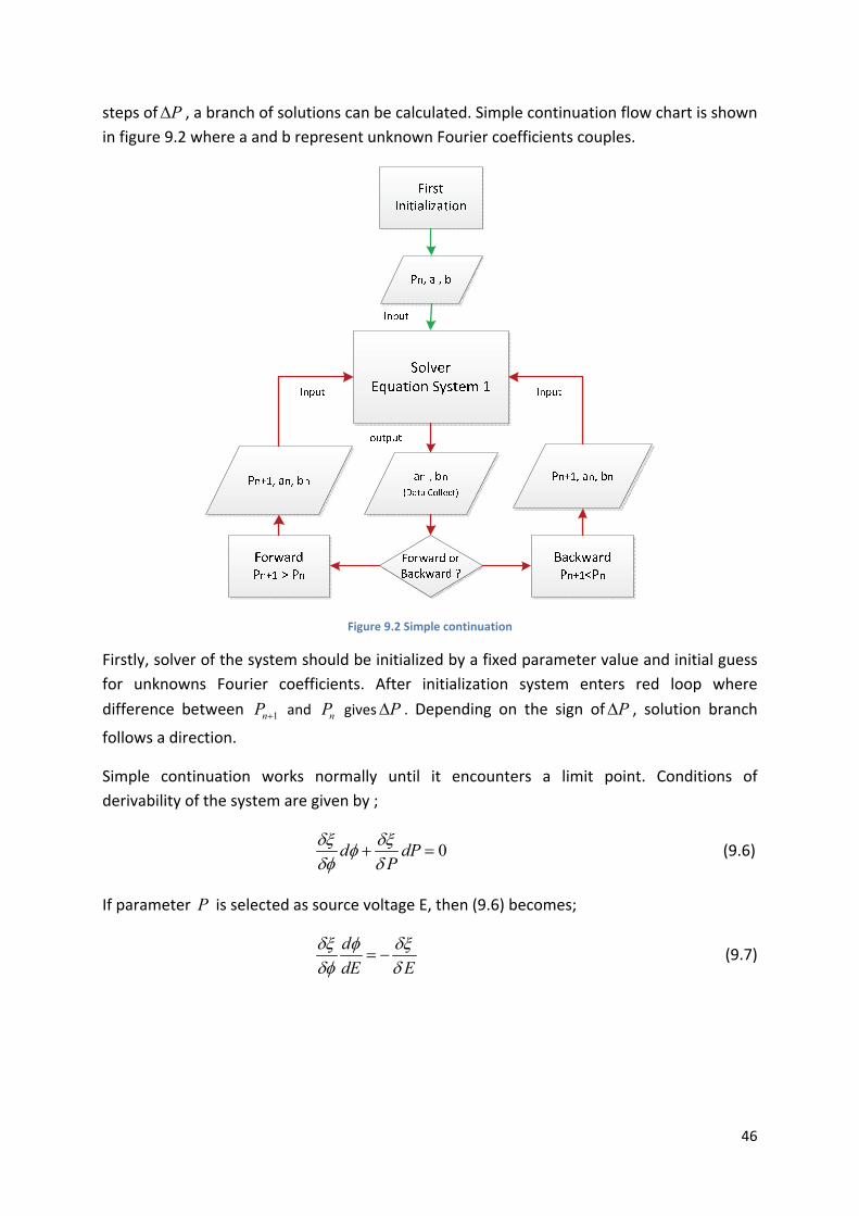
46
steps of P , a branch of solutions can be calculated. Simple continuation flow chart is shown
in figure 9.2 where a and b represent unknown Fourier coefficients couples.
Figure 9.2 Simple continuation
Firstly, solver of the system should be initialized by a fixed parameter value and initial guess
for unknowns Fourier coefficients. After initialization system enters red loop where
difference between 1nP and nP gives P . Depending on the sign of P , solution branch
follows a direction.
Simple continuation works normally until it encounters a limit point. Conditions of
derivability of the system are given by ;
0d dPP
(9.6)
If parameter P is selected as source voltage E, then (9.6) becomes;
d
dE E
(9.7)
47
Figure 9.3 Tangent at limit point
Tangent in figure 9.3 corresponds to d
dE
since 0dE while 0d .
When the Jacobean matrix
is singular (its determinant is zero by definition), the slope of
the tangent d
dE
to the curve is infinite [35],[36].
At these limit points, numerical harmonic balance method cannot converge since Jacobean
of the equation system gets singular. In order to turn these limit points and then continuate
the solution branch pseudo‐arc length continuation method is proposed by Kieny [35]. But in
this thesis another more simpler method is used which is called hyper‐sphere method [54].
By adding one more equation to the ( , ) 0 system, singularity at the limit point can be
overcome. Hence, complete curves can be drawn.
The new equation is a hyper‐sphere equation; a sphere that encloses a part of solution curve
always intersects the solution curve at least two times [54].
2 2 2 2 2 21 1 1 1( , , ) ( ) ( ) ... ( ) ( ) ( ) 0s c s sm c cm xs xsm xc xcm mg P P P r
(9.8)
m indices represents the known coefficient or parameter from last iteration.
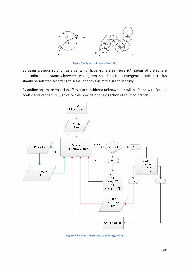
48
Figure 9.4 Hyper‐sphere method[54]
By using previous solution as a center of hyper‐sphere in figure 9.4, radius of the sphere
determines the distances between two adjacent solutions, for convergence problems radius
should be selected according to scales of both axis of the graph in study.
By adding one more equation, P is also considered unknown and will be found with Fourier
coefficients of the flux. Sign of P will decide on the direction of solution branch.
Figure 9.5 Hyper‐sphere continuation algorithm
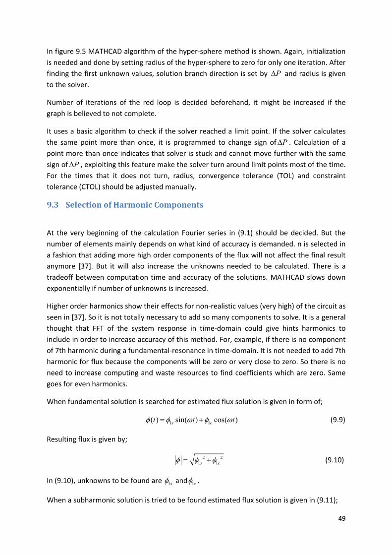
49
In figure 9.5 MATHCAD algorithm of the hyper‐sphere method is shown. Again, initialization
is needed and done by setting radius of the hyper‐sphere to zero for only one iteration. After
finding the first unknown values, solution branch direction is set by P and radius is given
to the solver.
Number of iterations of the red loop is decided beforehand, it might be increased if the
graph is believed to not complete.
It uses a basic algorithm to check if the solver reached a limit point. If the solver calculates
the same point more than once, it is programmed to change sign of P . Calculation of a
point more than once indicates that solver is stuck and cannot move further with the same
sign of P , exploiting this feature make the solver turn around limit points most of the time.
For the times that it does not turn, radius, convergence tolerance (TOL) and constraint
tolerance (CTOL) should be adjusted manually.
9.3 SelectionofHarmonicComponents
At the very beginning of the calculation Fourier series in (9.1) should be decided. But the
number of elements mainly depends on what kind of accuracy is demanded. n is selected in
a fashion that adding more high order components of the flux will not affect the final result
anymore [37]. But it will also increase the unknowns needed to be calculated. There is a
tradeoff between computation time and accuracy of the solutions. MATHCAD slows down
exponentially if number of unknowns is increased.
Higher order harmonics show their effects for non‐realistic values (very high) of the circuit as
seen in [37]. So it is not totally necessary to add so many components to solve. It is a general
thought that FFT of the system response in time‐domain could give hints harmonics to
include in order to increase accuracy of this method. For, example, if there is no component
of 7th harmonic during a fundamental‐resonance in time‐domain. It is not needed to add 7th
harmonic for flux because the components will be zero or very close to zero. So there is no
need to increase computing and waste resources to find coefficients which are zero. Same
goes for even harmonics.
When fundamental solution is searched for estimated flux solution is given in form of;
1 1( ) sin( ) cos( )s ct t t (9.9)
Resulting flux is given by;
2 2
1 1s c (9.10)
In (9.10), unknowns to be found are 1s and 1c .
When a subharmonic solution is tried to be found estimated flux solution is given in (9.11);
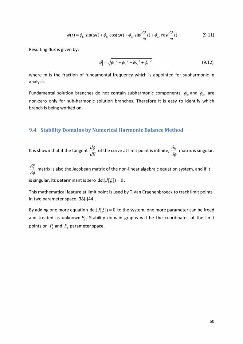
50
1 1 2 2( ) sin( ) cos( ) sin( ) cos( )s c s ct t t t t
m m
(9.11)
Resulting flux is given by;
2 2 2 2
1 1 2 2s c s c (9.12)
where m is the fraction of fundamental frequency which is appointed for subharmonic in
analysis.
Fundamental solution branches do not contain subharmonic components. 2s and 2c are
non‐zero only for sub‐harmonic solution branches. Therefore it is easy to identify which
branch is being worked on.
9.4 StabilityDomainsbyNumericalHarmonicBalanceMethod
It is shown that if the tangent d
dE
of the curve at limit point is infinite,
matrix is singular.
matrix is also the Jacobean matrix of the non‐linear algebraic equation system, and if it
is singular, its determinant is zero det( [ ]) 0J .
This mathematical feature at limit point is used by T.Van Craenenbroeck to track limit points
in two parameter space [38]‐[44].
By adding one more equation det( [ ]) 0J to the system, one more parameter can be freed
and treated as unknown 2P . Stability domain graphs will be the coordinates of the limit
points on 1P and 2P parameter space.
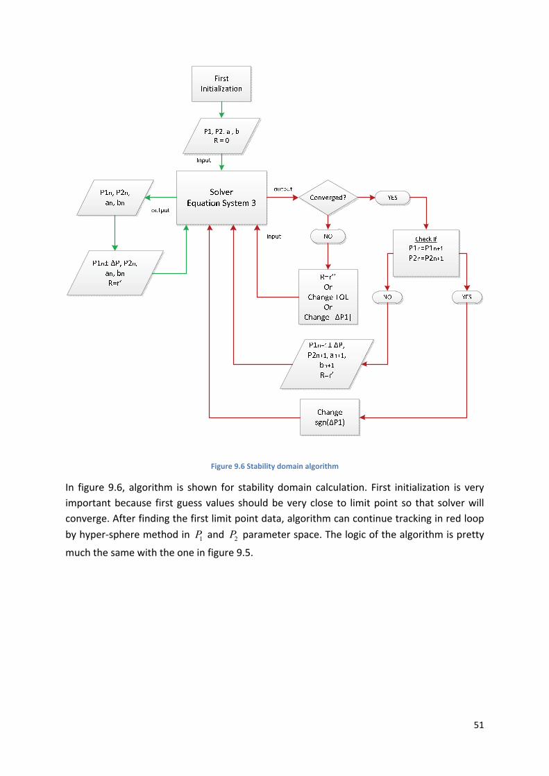
51
Figure 9.6 Stability domain algorithm
In figure 9.6, algorithm is shown for stability domain calculation. First initialization is very
important because first guess values should be very close to limit point so that solver will
converge. After finding the first limit point data, algorithm can continue tracking in red loop
by hyper‐sphere method in 1P and 2P parameter space. The logic of the algorithm is pretty
much the same with the one in figure 9.5.
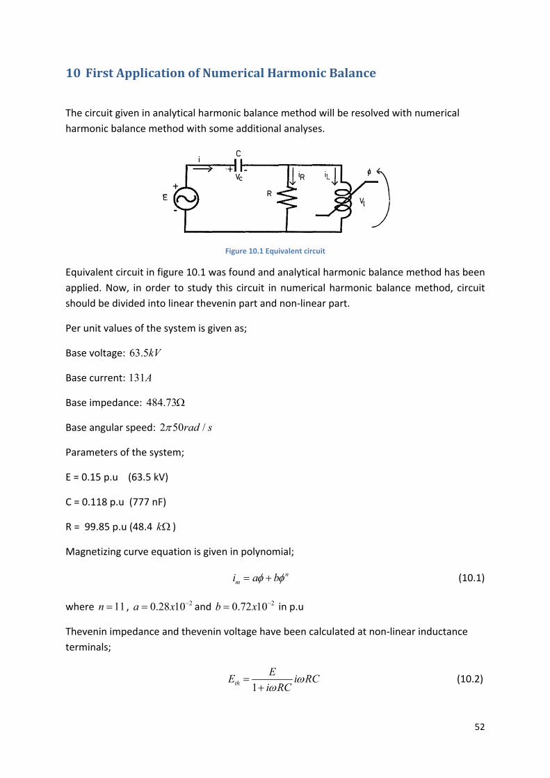
52
10 FirstApplicationofNumericalHarmonicBalance
The circuit given in analytical harmonic balance method will be resolved with numerical
harmonic balance method with some additional analyses.
Figure 10.1 Equivalent circuit
Equivalent circuit in figure 10.1 was found and analytical harmonic balance method has been
applied. Now, in order to study this circuit in numerical harmonic balance method, circuit
should be divided into linear thevenin part and non‐linear part.
Per unit values of the system is given as;
Base voltage: 63.5kV
Base current: 131A
Base impedance: 484.73
Base angular speed: 2 50 /rad s
Parameters of the system;
E = 0.15 p.u (63.5 kV)
C = 0.118 p.u (777 nF)
R = 99.85 p.u (48.4 k )
Magnetizing curve equation is given in polynomial;
nmi a b (10.1)
where 11n , 20.28 10a x and 20.72 10b x in p.u
Thevenin impedance and thevenin voltage have been calculated at non‐linear inductance
terminals;
1th
EE i RC
i RC
(10.2)
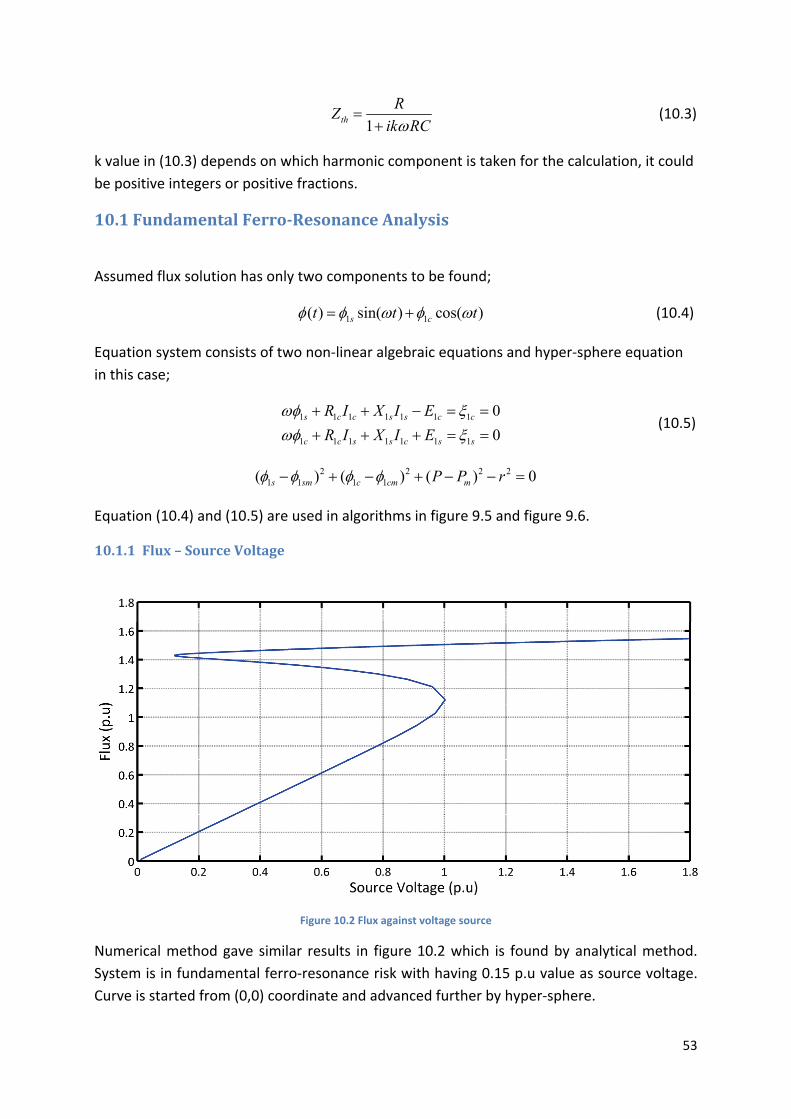
53
1th
RZ
ik RC
(10.3)
k value in (10.3) depends on which harmonic component is taken for the calculation, it could
be positive integers or positive fractions.
10.1 FundamentalFerro‐ResonanceAnalysis
Assumed flux solution has only two components to be found;
1 1( ) sin( ) cos( )s ct t t (10.4)
Equation system consists of two non‐linear algebraic equations and hyper‐sphere equation
in this case;
1 1 1 1 1 1 1
1 1 1 1 1 1 1
0
0s c c s s c c
c c s s c s s
R I X I E
R I X I E
(10.5)
2 2 2 21 1 1 1( ) ( ) ( ) 0s sm c cm mP P r
Equation (10.4) and (10.5) are used in algorithms in figure 9.5 and figure 9.6.
10.1.1 Flux–SourceVoltage
Figure 10.2 Flux against voltage source
Numerical method gave similar results in figure 10.2 which is found by analytical method.
System is in fundamental ferro‐resonance risk with having 0.15 p.u value as source voltage.
Curve is started from (0,0) coordinate and advanced further by hyper‐sphere.
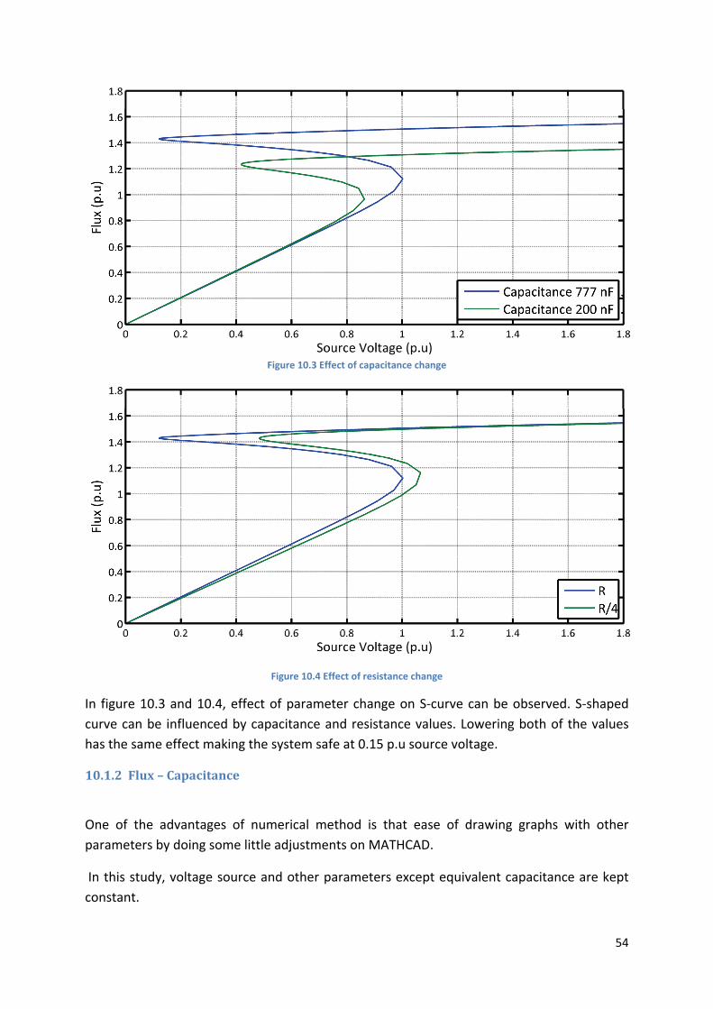
54
Figure 10.3 Effect of capacitance change
Figure 10.4 Effect of resistance change
In figure 10.3 and 10.4, effect of parameter change on S‐curve can be observed. S‐shaped
curve can be influenced by capacitance and resistance values. Lowering both of the values
has the same effect making the system safe at 0.15 p.u source voltage.
10.1.2 Flux–Capacitance
One of the advantages of numerical method is that ease of drawing graphs with other
parameters by doing some little adjustments on MATHCAD.
In this study, voltage source and other parameters except equivalent capacitance are kept
constant.
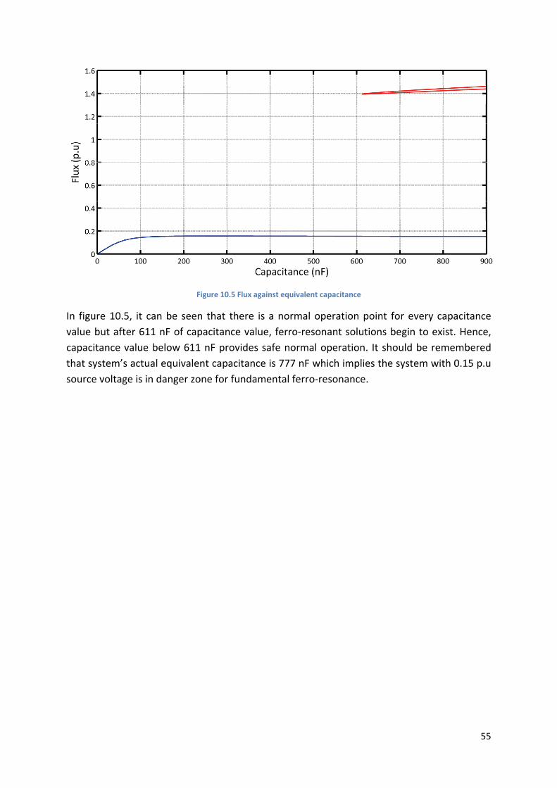
55
Figure 10.5 Flux against equivalent capacitance
In figure 10.5, it can be seen that there is a normal operation point for every capacitance
value but after 611 nF of capacitance value, ferro‐resonant solutions begin to exist. Hence,
capacitance value below 611 nF provides safe normal operation. It should be remembered
that system’s actual equivalent capacitance is 777 nF which implies the system with 0.15 p.u
source voltage is in danger zone for fundamental ferro‐resonance.
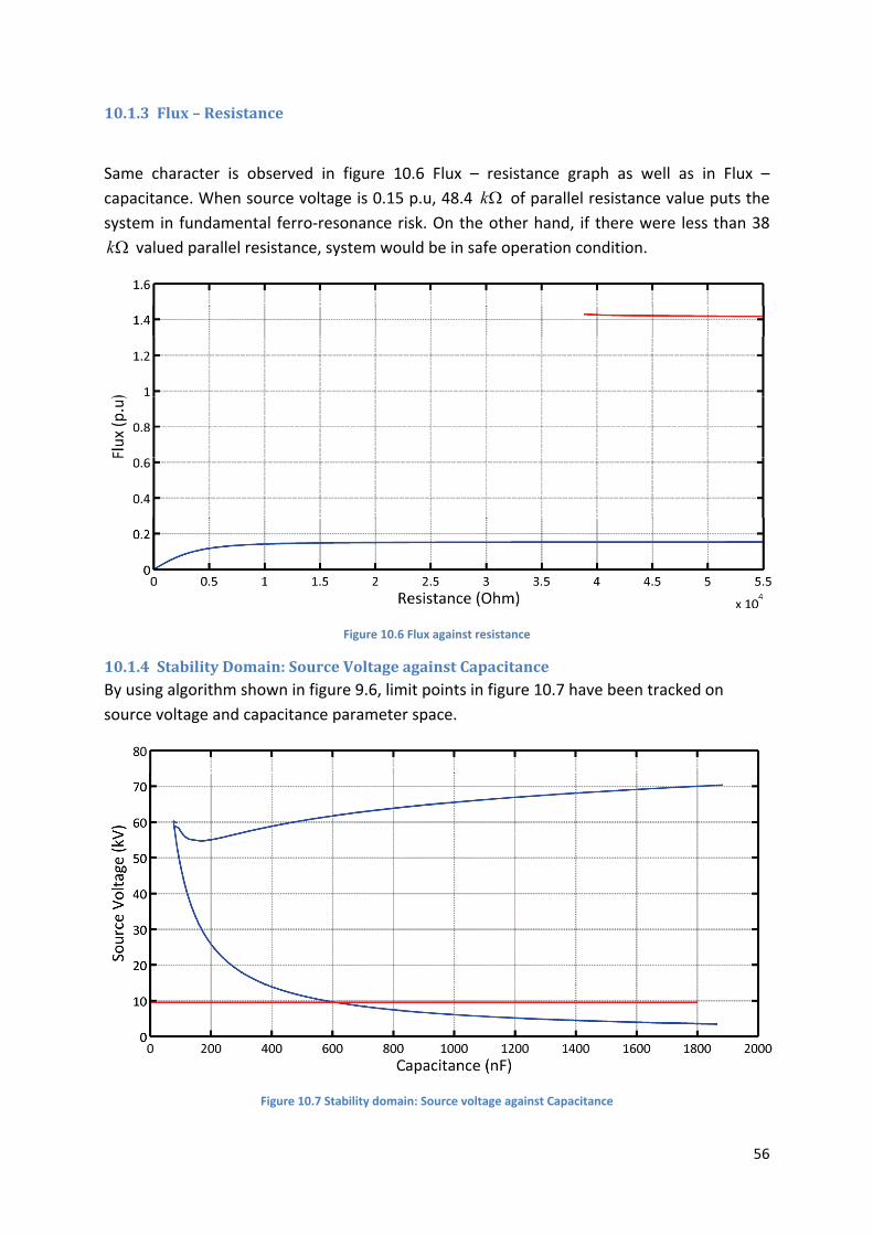
56
10.1.3 Flux–Resistance
Same character is observed in figure 10.6 Flux – resistance graph as well as in Flux –
capacitance. When source voltage is 0.15 p.u, 48.4 k of parallel resistance value puts the
system in fundamental ferro‐resonance risk. On the other hand, if there were less than 38
k valued parallel resistance, system would be in safe operation condition.
Figure 10.6 Flux against resistance
10.1.4 StabilityDomain:SourceVoltageagainstCapacitanceBy using algorithm shown in figure 9.6, limit points in figure 10.7 have been tracked on
source voltage and capacitance parameter space.
Figure 10.7 Stability domain: Source voltage against Capacitance
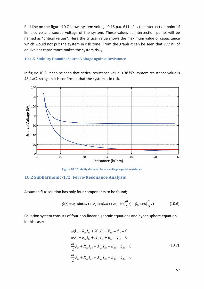
57
Red line on the figure 10.7 shows system voltage 0.15 p.u. 611 nF is the intersection point of
limit curve and source voltage of the system. These values at intersection points will be
named as “critical values”. Here the critical value shows the maximum value of capacitance
which would not put the system in risk zone. From the graph it can be seen that 777 nF of
equivalent capacitance makes the system risky.
10.1.5 StabilityDomain:SourceVoltageagainstResistance
In figure 10.8, it can be seen that critical resistance value is 38 k , system resistance value is
48.4 k so again it is confirmed that the system is in risk.
Figure 10.8 Stability domain: Source voltage against resistance
10.2 Subharmonic‐1/2Ferro‐ResonanceAnalysis
Assumed flux solution has only four components to be found;
1 1 2 2( ) sin( ) cos( ) sin( ) cos( )2 2s c s ct t t t t (10.6)
Equation system consists of four non‐linear algebraic equations and hyper‐sphere equation
in this case;
1 1 1 1 1 1 1
1 1 1 1 1 1 1
2 2 2 2 2 2 2
2 2 2 2 2 2 2
0
0
02
02
s c c s s c c
c c s s c s s
s c c s s c c
c c s s c s s
R I X I E
R I X I E
R I X I E
R I X I E
(10.7)
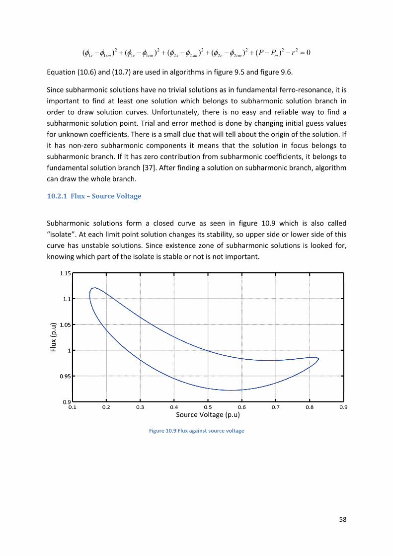
58
2 2 2 2 2 21 1 1 1 2 2 2 2( ) ( ) ( ) ( ) ( ) 0s sm c cm s sm c cm mP P r
Equation (10.6) and (10.7) are used in algorithms in figure 9.5 and figure 9.6.
Since subharmonic solutions have no trivial solutions as in fundamental ferro‐resonance, it is
important to find at least one solution which belongs to subharmonic solution branch in
order to draw solution curves. Unfortunately, there is no easy and reliable way to find a
subharmonic solution point. Trial and error method is done by changing initial guess values
for unknown coefficients. There is a small clue that will tell about the origin of the solution. If
it has non‐zero subharmonic components it means that the solution in focus belongs to
subharmonic branch. If it has zero contribution from subharmonic coefficients, it belongs to
fundamental solution branch [37]. After finding a solution on subharmonic branch, algorithm
can draw the whole branch.
10.2.1 Flux–SourceVoltage
Subharmonic solutions form a closed curve as seen in figure 10.9 which is also called
“isolate”. At each limit point solution changes its stability, so upper side or lower side of this
curve has unstable solutions. Since existence zone of subharmonic solutions is looked for,
knowing which part of the isolate is stable or not is not important.
Figure 10.9 Flux against source voltage
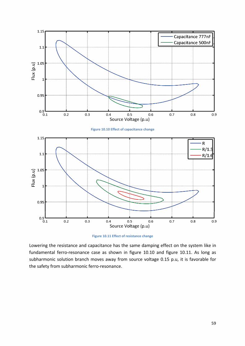
59
Figure 10.10 Effect of capacitance change
Figure 10.11 Effect of resistance change
Lowering the resistance and capacitance has the same damping effect on the system like in
fundamental ferro‐resonance case as shown in figure 10.10 and figure 10.11. As long as
subharmonic solution branch moves away from source voltage 0.15 p.u, it is favorable for
the safety from subharmonic ferro‐resonance.
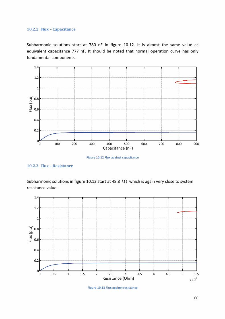
60
10.2.2 Flux–Capacitance
Subharmonic solutions start at 780 nF in figure 10.12. It is almost the same value as
equivalent capacitance 777 nF. It should be noted that normal operation curve has only
fundamental components.
Figure 10.12 Flux against capacitance
10.2.3 Flux–Resistance
Subharmonic solutions in figure 10.13 start at 48.8 k which is again very close to system
resistance value.
Figure 10.13 Flux against resistance
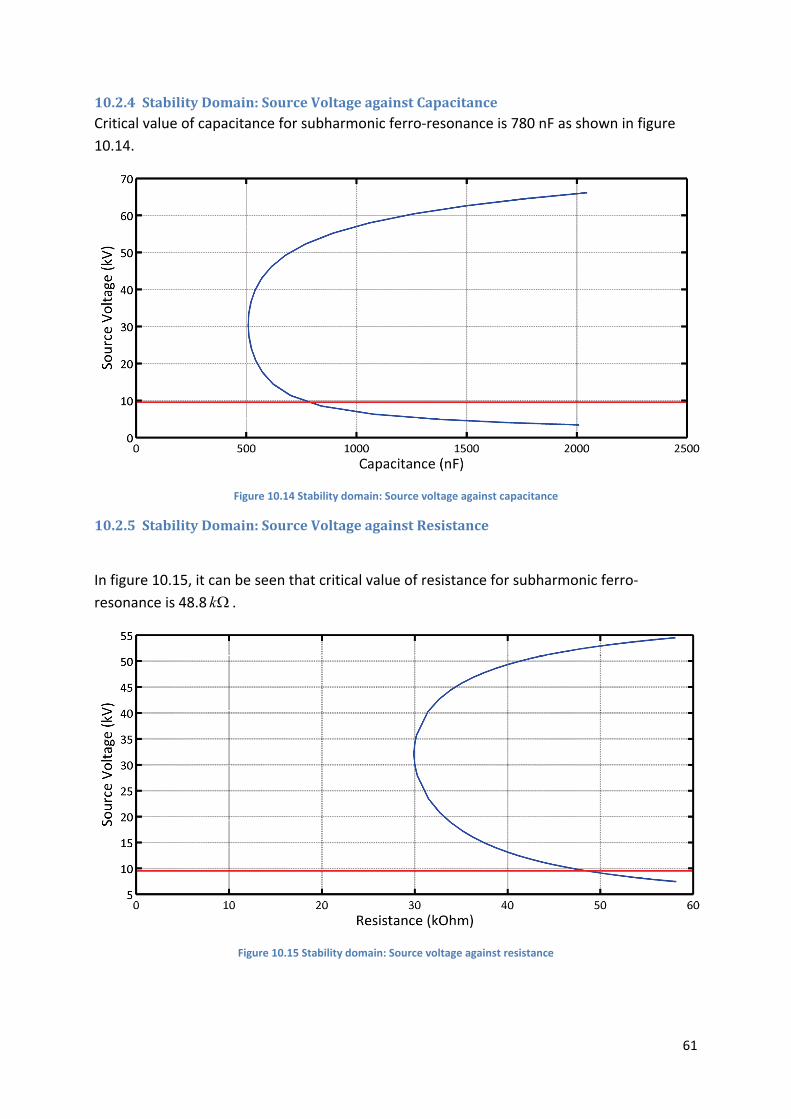
61
10.2.4 StabilityDomain:SourceVoltageagainstCapacitanceCritical value of capacitance for subharmonic ferro‐resonance is 780 nF as shown in figure
10.14.
Figure 10.14 Stability domain: Source voltage against capacitance
10.2.5 StabilityDomain:SourceVoltageagainstResistance
In figure 10.15, it can be seen that critical value of resistance for subharmonic ferro‐
resonance is 48.8 k .
Figure 10.15 Stability domain: Source voltage against resistance
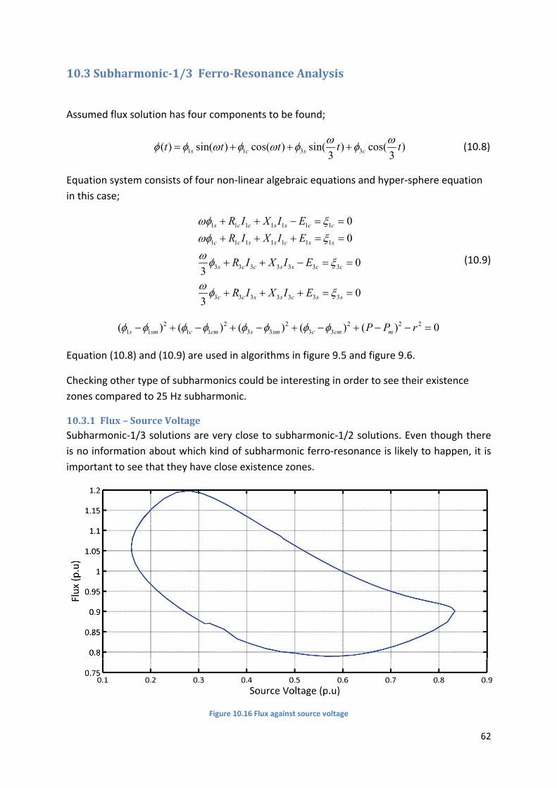
62
10.3 Subharmonic‐1/3Ferro‐ResonanceAnalysis
Assumed flux solution has four components to be found;
1 1 3 3( ) sin( ) cos( ) sin( ) cos( )3 3s c s ct t t t t (10.8)
Equation system consists of four non‐linear algebraic equations and hyper‐sphere equation
in this case;
1 1 1 1 1 1 1
1 1 1 1 1 1 1
3 3 3 3 3 3 3
3 3 3 3 3 3 3
0
0
03
03
s c c s s c c
c c s s c s s
s c c s s c c
c c s s c s s
R I X I E
R I X I E
R I X I E
R I X I E
(10.9)
2 2 2 2 2 21 1 1 1 3 3 3 3( ) ( ) ( ) ( ) ( ) 0s sm c cm s sm c cm mP P r
Equation (10.8) and (10.9) are used in algorithms in figure 9.5 and figure 9.6.
Checking other type of subharmonics could be interesting in order to see their existence
zones compared to 25 Hz subharmonic.
10.3.1 Flux–SourceVoltageSubharmonic‐1/3 solutions are very close to subharmonic‐1/2 solutions. Even though there
is no information about which kind of subharmonic ferro‐resonance is likely to happen, it is
important to see that they have close existence zones.
Figure 10.16 Flux against source voltage
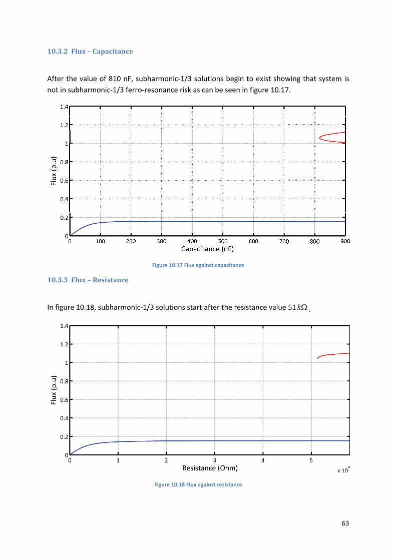
10.3.2 F
After th
not in s
10.3.3 F
In figure
Flux–Capa
he value of
ubharmonic
Flux–Resis
e 10.18, sub
acitance
810 nF, su
c‐1/3 ferro‐
stance
bharmonic‐
bharmonic‐
‐resonance
Figure 10.1
1/3 solution
Figure 10.
‐1/3 solutio
risk as can
17 Flux against
ns start afte
18 Flux against
ons begin to
be seen in f
capacitance
er the resist
t resistance
o exist show
figure 10.17
tance value
wing that sy
7.
51 k .
63
ystem is
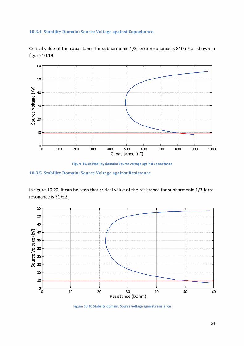
64
10.3.4 StabilityDomain:SourceVoltageagainstCapacitance
Critical value of the capacitance for subharmonic‐1/3 ferro‐resonance is 810 nF as shown in
figure 10.19.
Figure 10.19 Stability domain: Source voltage against capacitance
10.3.5 StabilityDomain:SourceVoltageagainstResistance
In figure 10.20, it can be seen that critical value of the resistance for subharmonic‐1/3 ferro‐
resonance is 51 k .
Figure 10.20 Stability domain: Source voltage against resistance
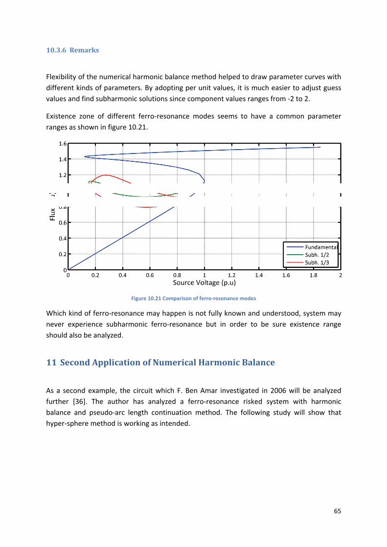
65
10.3.6 Remarks
Flexibility of the numerical harmonic balance method helped to draw parameter curves with
different kinds of parameters. By adopting per unit values, it is much easier to adjust guess
values and find subharmonic solutions since component values ranges from ‐2 to 2.
Existence zone of different ferro‐resonance modes seems to have a common parameter
ranges as shown in figure 10.21.
Figure 10.21 Comparison of ferro‐resonance modes
Which kind of ferro‐resonance may happen is not fully known and understood, system may
never experience subharmonic ferro‐resonance but in order to be sure existence range
should also be analyzed.
11 SecondApplicationofNumericalHarmonicBalance
As a second example, the circuit which F. Ben Amar investigated in 2006 will be analyzed
further [36]. The author has analyzed a ferro‐resonance risked system with harmonic
balance and pseudo‐arc length continuation method. The following study will show that
hyper‐sphere method is working as intended.
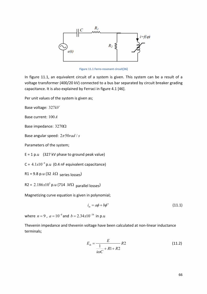
66
Figure 11.1 Ferro‐resonant circuit[36]
In figure 11.1, an equivalent circuit of a system is given. This system can be a result of a
voltage transformer (400/20 kV) connected to a bus bar separated by circuit breaker grading
capacitance. It is also explained by Ferraci in figure 4.1 [46].
Per unit values of the system is given as;
Base voltage: 327kV
Base current: 100A
Base impedance: 3270
Base angular speed: 2 50 /rad s
Parameters of the system;
E = 1 p.u (327 kV phase to ground peak value)
C = 44.1 10x p.u (0.4 nF equivalent capacitance)
R1 = 9.8 p.u (32 k series losses)
R2 = 52.186 10x p.u (714 M parallel losses)
Magnetizing curve equation is given in polynomial;
nmi a b (11.1)
where 9n , 810a and 342.34 10b x in p.u
Thevenin impedance and thevenin voltage have been calculated at non‐linear inductance
terminals;
21
1 2th
EE R
R Ri C
(11.2)
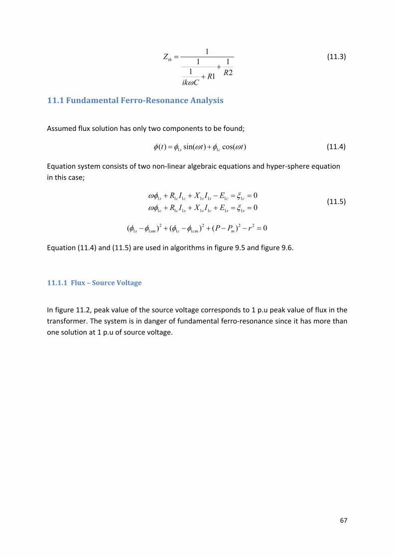
67
1
1 11 21
thZ
RRik C
(11.3)
11.1 FundamentalFerro‐ResonanceAnalysis
Assumed flux solution has only two components to be found;
1 1( ) sin( ) cos( )s ct t t (11.4)
Equation system consists of two non‐linear algebraic equations and hyper‐sphere equation
in this case;
1 1 1 1 1 1 1
1 1 1 1 1 1 1
0
0s c c s s c c
c c s s c s s
R I X I E
R I X I E
(11.5)
2 2 2 21 1 1 1( ) ( ) ( ) 0s sm c cm mP P r
Equation (11.4) and (11.5) are used in algorithms in figure 9.5 and figure 9.6.
11.1.1 Flux–SourceVoltage
In figure 11.2, peak value of the source voltage corresponds to 1 p.u peak value of flux in the
transformer. The system is in danger of fundamental ferro‐resonance since it has more than
one solution at 1 p.u of source voltage.
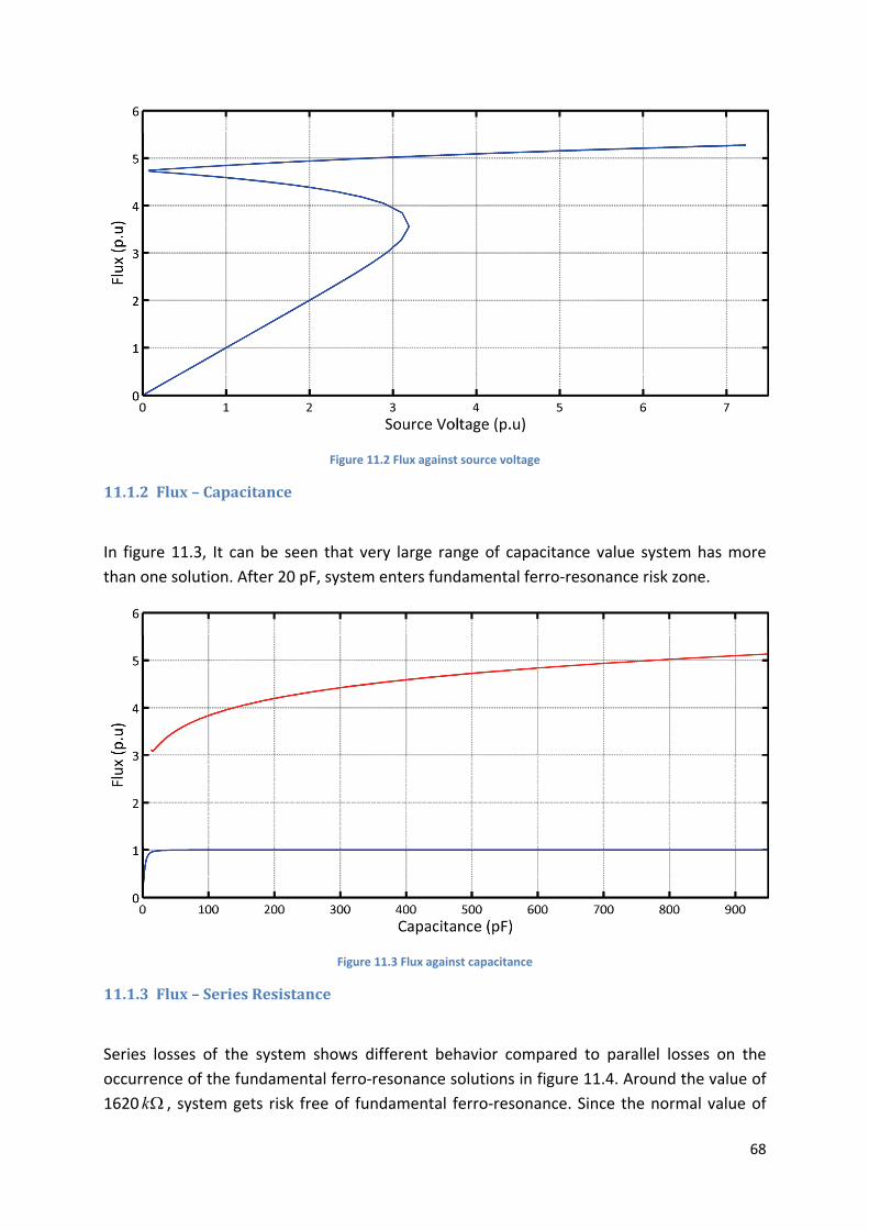
68
Figure 11.2 Flux against source voltage
11.1.2 Flux–Capacitance
In figure 11.3, It can be seen that very large range of capacitance value system has more
than one solution. After 20 pF, system enters fundamental ferro‐resonance risk zone.
Figure 11.3 Flux against capacitance
11.1.3 Flux–SeriesResistance
Series losses of the system shows different behavior compared to parallel losses on the
occurrence of the fundamental ferro‐resonance solutions in figure 11.4. Around the value of
1620 k , system gets risk free of fundamental ferro‐resonance. Since the normal value of
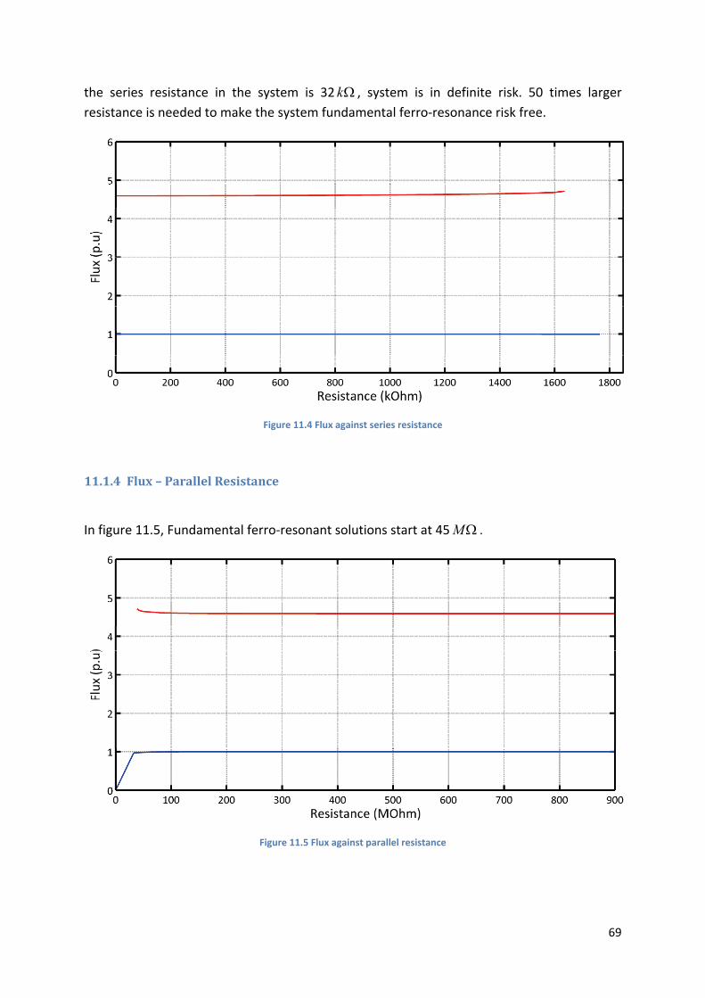
69
the series resistance in the system is 32 k , system is in definite risk. 50 times larger
resistance is needed to make the system fundamental ferro‐resonance risk free.
Figure 11.4 Flux against series resistance
11.1.4 Flux–ParallelResistance
In figure 11.5, Fundamental ferro‐resonant solutions start at 45M .
Figure 11.5 Flux against parallel resistance
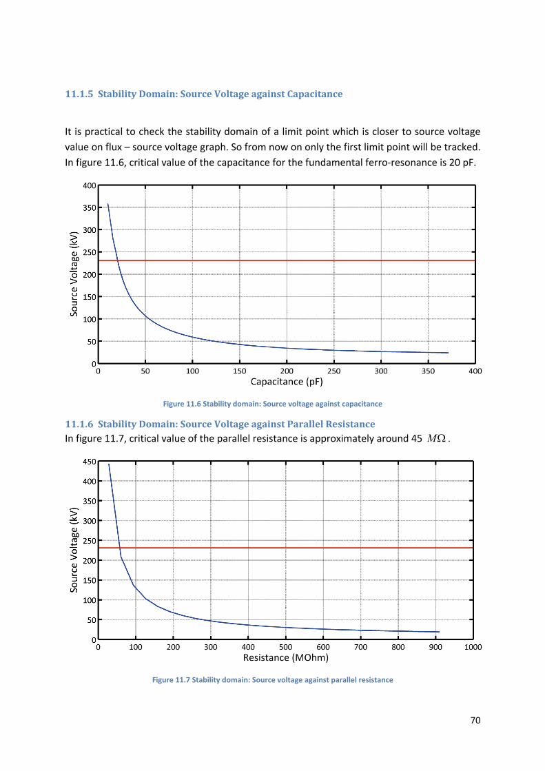
70
11.1.5 StabilityDomain:SourceVoltageagainstCapacitance
It is practical to check the stability domain of a limit point which is closer to source voltage
value on flux – source voltage graph. So from now on only the first limit point will be tracked.
In figure 11.6, critical value of the capacitance for the fundamental ferro‐resonance is 20 pF.
Figure 11.6 Stability domain: Source voltage against capacitance
11.1.6 StabilityDomain:SourceVoltageagainstParallelResistanceIn figure 11.7, critical value of the parallel resistance is approximately around 45 M .
Figure 11.7 Stability domain: Source voltage against parallel resistance
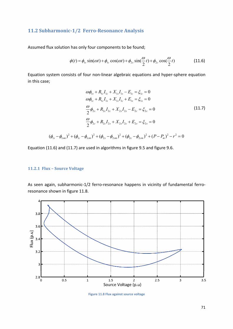
71
11.2 Subharmonic‐1/2Ferro‐ResonanceAnalysis
Assumed flux solution has only four components to be found;
1 1 2 2( ) sin( ) cos( ) sin( ) cos( )2 2s c s ct t t t t (11.6)
Equation system consists of four non‐linear algebraic equations and hyper‐sphere equation
in this case;
1 1 1 1 1 1 1
1 1 1 1 1 1 1
2 2 2 2 2 2 2
2 2 2 2 2 2 2
0
0
02
02
s c c s s c c
c c s s c s s
s c c s s c c
c c s s c s s
R I X I E
R I X I E
R I X I E
R I X I E
(11.7)
2 2 2 2 2 21 1 1 1 2 2 2 2( ) ( ) ( ) ( ) ( ) 0s sm c cm s sm c cm mP P r
Equation (11.6) and (11.7) are used in algorithms in figure 9.5 and figure 9.6.
11.2.1 Flux–SourceVoltage
As seen again, subharmonic‐1/2 ferro‐resonance happens in vicinity of fundamental ferro‐
resonance shown in figure 11.8.
Figure 11.8 Flux against source voltage
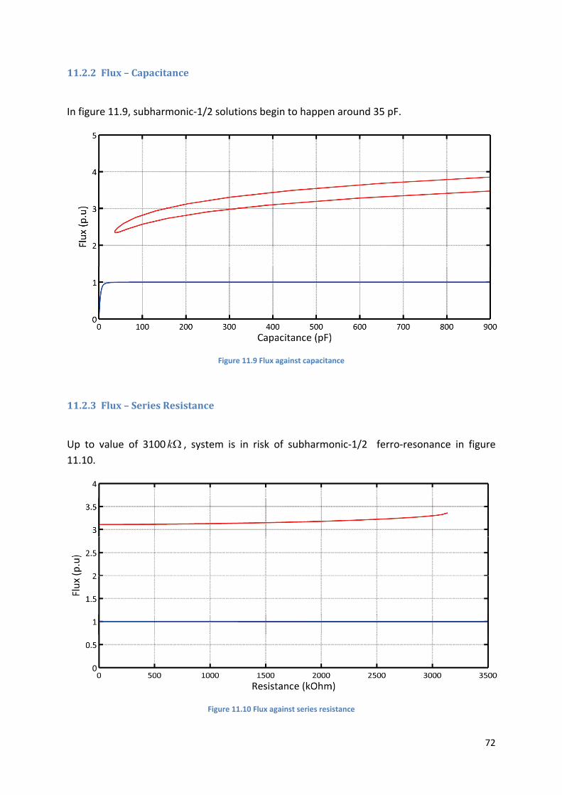
72
11.2.2 Flux–Capacitance
In figure 11.9, subharmonic‐1/2 solutions begin to happen around 35 pF.
Figure 11.9 Flux against capacitance
11.2.3 Flux–SeriesResistance
Up to value of 3100 k , system is in risk of subharmonic‐1/2 ferro‐resonance in figure
11.10.
Figure 11.10 Flux against series resistance
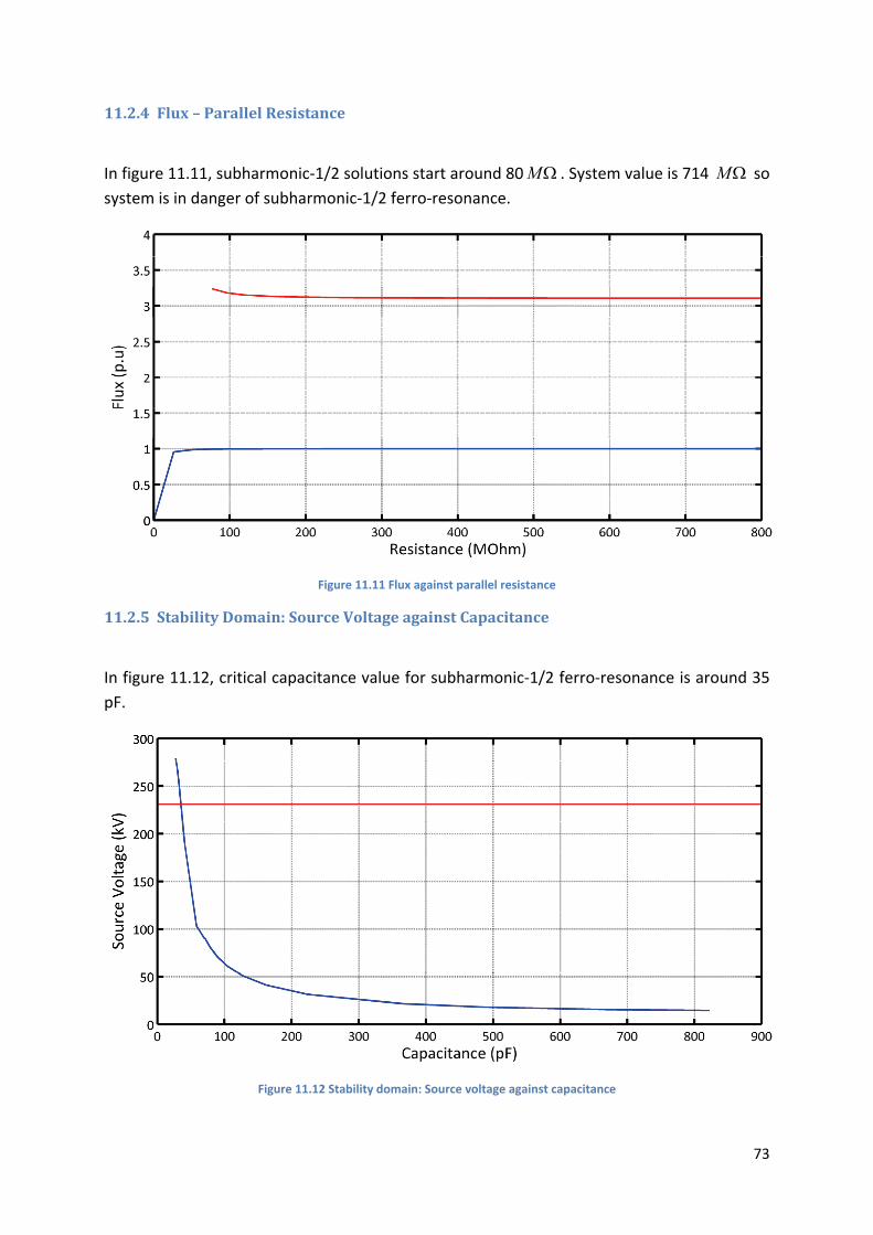
73
11.2.4 Flux–ParallelResistance
In figure 11.11, subharmonic‐1/2 solutions start around 80M . System value is 714 M so
system is in danger of subharmonic‐1/2 ferro‐resonance.
Figure 11.11 Flux against parallel resistance
11.2.5 StabilityDomain:SourceVoltageagainstCapacitance
In figure 11.12, critical capacitance value for subharmonic‐1/2 ferro‐resonance is around 35
pF.
Figure 11.12 Stability domain: Source voltage against capacitance
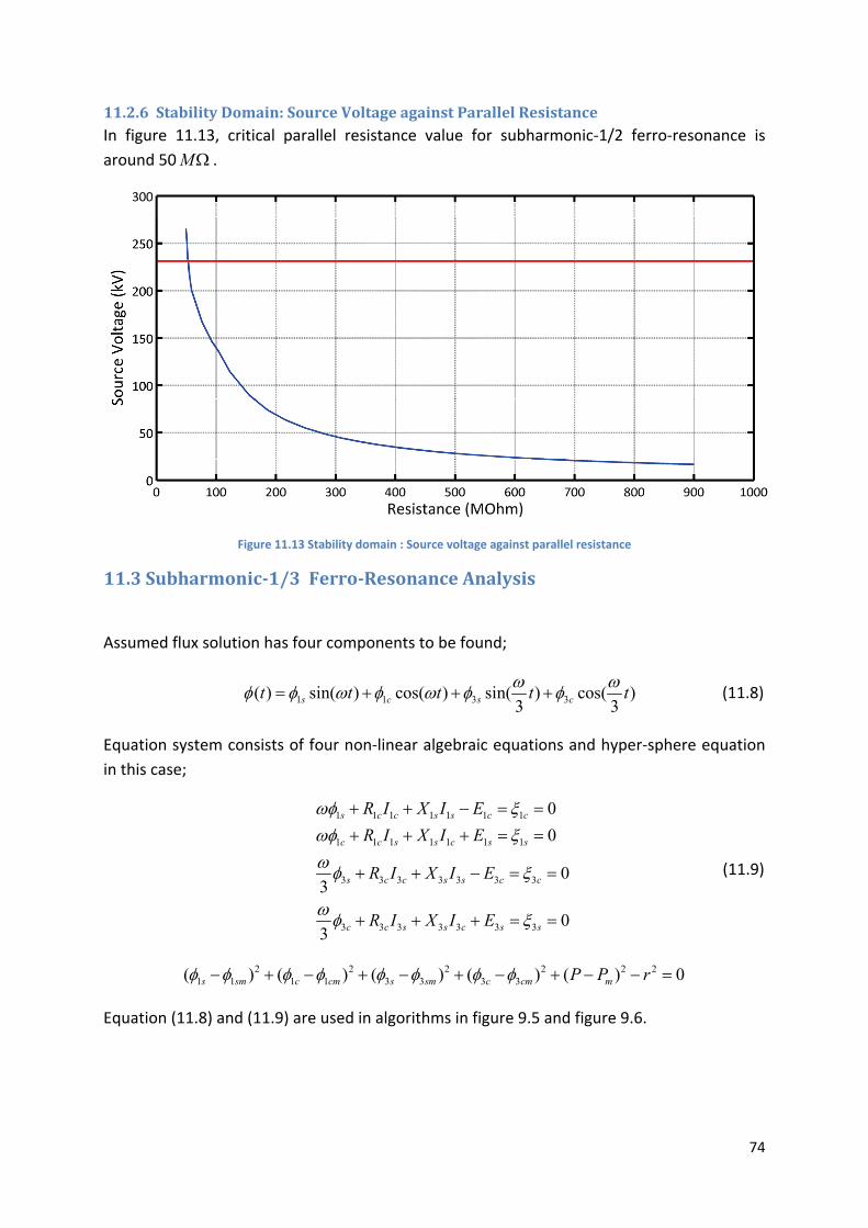
74
11.2.6 StabilityDomain:SourceVoltageagainstParallelResistanceIn figure 11.13, critical parallel resistance value for subharmonic‐1/2 ferro‐resonance is
around 50M .
Figure 11.13 Stability domain : Source voltage against parallel resistance
11.3 Subharmonic‐1/3Ferro‐ResonanceAnalysis
Assumed flux solution has four components to be found;
1 1 3 3( ) sin( ) cos( ) sin( ) cos( )3 3s c s ct t t t t (11.8)
Equation system consists of four non‐linear algebraic equations and hyper‐sphere equation
in this case;
1 1 1 1 1 1 1
1 1 1 1 1 1 1
3 3 3 3 3 3 3
3 3 3 3 3 3 3
0
0
03
03
s c c s s c c
c c s s c s s
s c c s s c c
c c s s c s s
R I X I E
R I X I E
R I X I E
R I X I E
(11.9)
2 2 2 2 2 21 1 1 1 3 3 3 3( ) ( ) ( ) ( ) ( ) 0s sm c cm s sm c cm mP P r
Equation (11.8) and (11.9) are used in algorithms in figure 9.5 and figure 9.6.
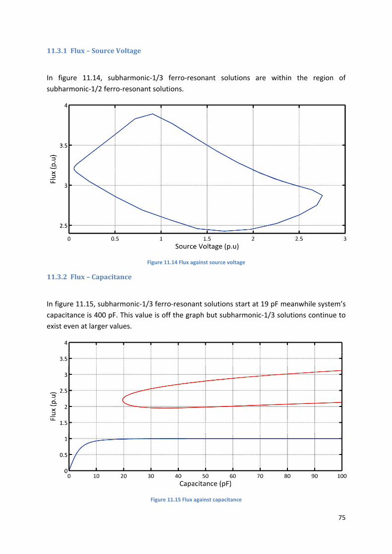
75
11.3.1 Flux–SourceVoltage
In figure 11.14, subharmonic‐1/3 ferro‐resonant solutions are within the region of
subharmonic‐1/2 ferro‐resonant solutions.
Figure 11.14 Flux against source voltage
11.3.2 Flux–Capacitance
In figure 11.15, subharmonic‐1/3 ferro‐resonant solutions start at 19 pF meanwhile system’s
capacitance is 400 pF. This value is off the graph but subharmonic‐1/3 solutions continue to
exist even at larger values.
Figure 11.15 Flux against capacitance
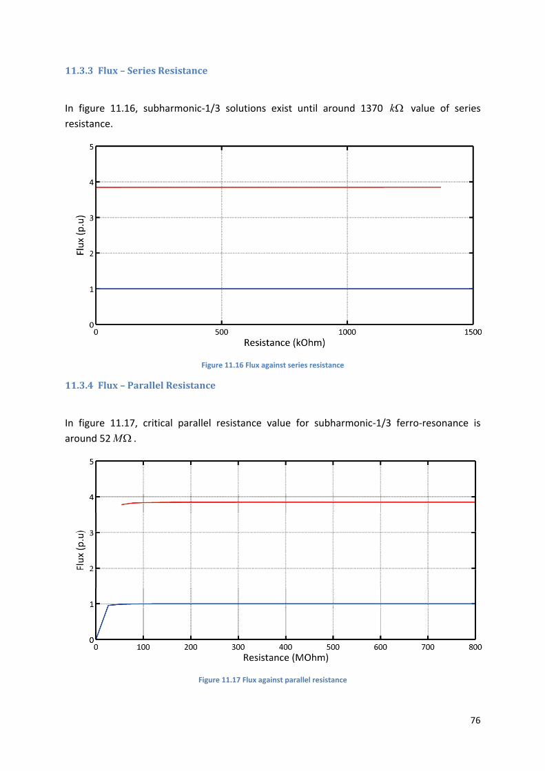
76
11.3.3 Flux–SeriesResistance
In figure 11.16, subharmonic‐1/3 solutions exist until around 1370 k value of series
resistance.
Figure 11.16 Flux against series resistance
11.3.4 Flux–ParallelResistance
In figure 11.17, critical parallel resistance value for subharmonic‐1/3 ferro‐resonance is
around 52M .
Figure 11.17 Flux against parallel resistance
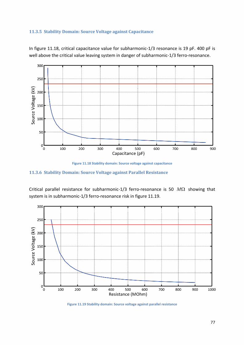
77
11.3.5 StabilityDomain:SourceVoltageagainstCapacitance
In figure 11.18, critical capacitance value for subharmonic‐1/3 resonance is 19 pF. 400 pF is
well above the critical value leaving system in danger of subharmonic‐1/3 ferro‐resonance.
Figure 11.18 Stability domain: Source voltage against capacitance
11.3.6 StabilityDomain:SourceVoltageagainstParallelResistance
Critical parallel resistance for subharmonic‐1/3 ferro‐resonance is 50 M showing that
system is in subharmonic‐1/3 ferro‐resonance risk in figure 11.19.
Figure 11.19 Stability domain: Source voltage against parallel resistance
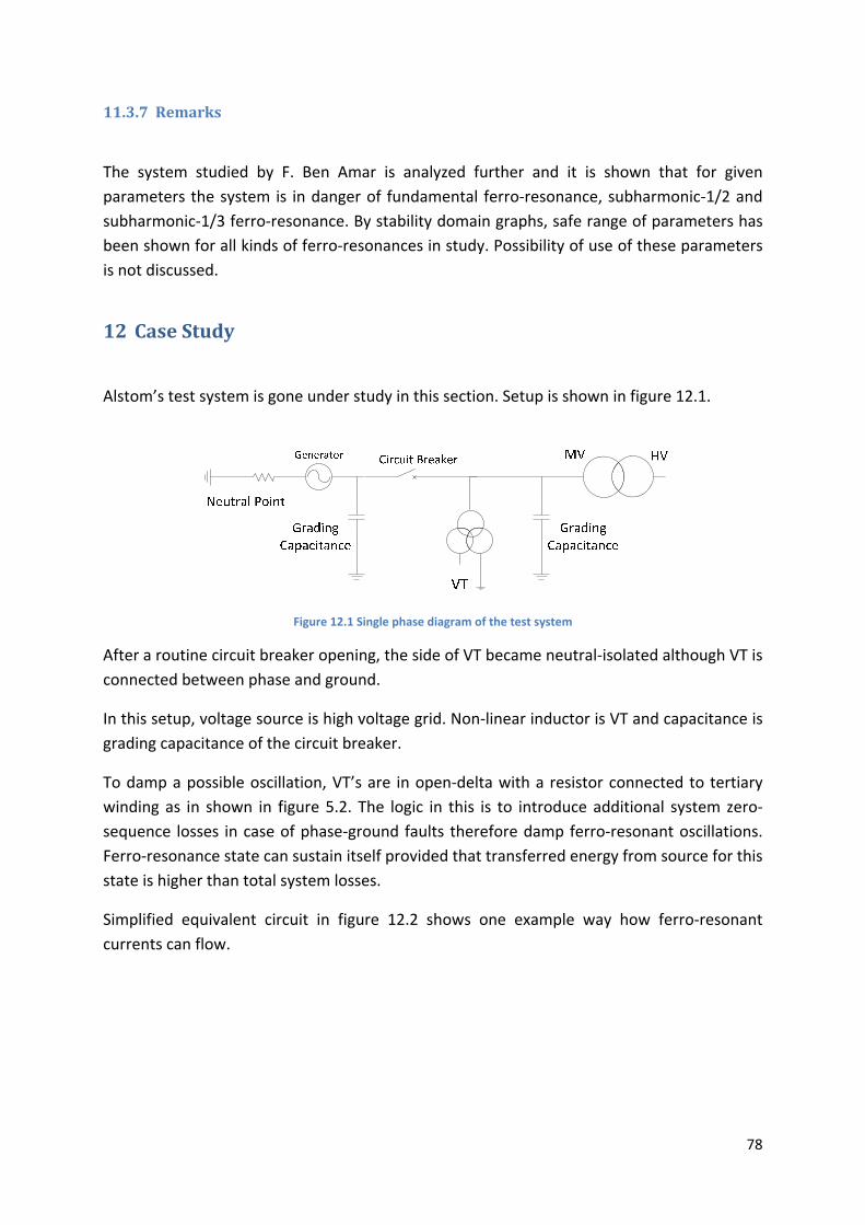
78
11.3.7 Remarks
The system studied by F. Ben Amar is analyzed further and it is shown that for given
parameters the system is in danger of fundamental ferro‐resonance, subharmonic‐1/2 and
subharmonic‐1/3 ferro‐resonance. By stability domain graphs, safe range of parameters has
been shown for all kinds of ferro‐resonances in study. Possibility of use of these parameters
is not discussed.
12 CaseStudy
Alstom’s test system is gone under study in this section. Setup is shown in figure 12.1.
Figure 12.1 Single phase diagram of the test system
After a routine circuit breaker opening, the side of VT became neutral‐isolated although VT is
connected between phase and ground.
In this setup, voltage source is high voltage grid. Non‐linear inductor is VT and capacitance is
grading capacitance of the circuit breaker.
To damp a possible oscillation, VT’s are in open‐delta with a resistor connected to tertiary
winding as in shown in figure 5.2. The logic in this is to introduce additional system zero‐
sequence losses in case of phase‐ground faults therefore damp ferro‐resonant oscillations.
Ferro‐resonance state can sustain itself provided that transferred energy from source for this
state is higher than total system losses.
Simplified equivalent circuit in figure 12.2 shows one example way how ferro‐resonant
currents can flow.
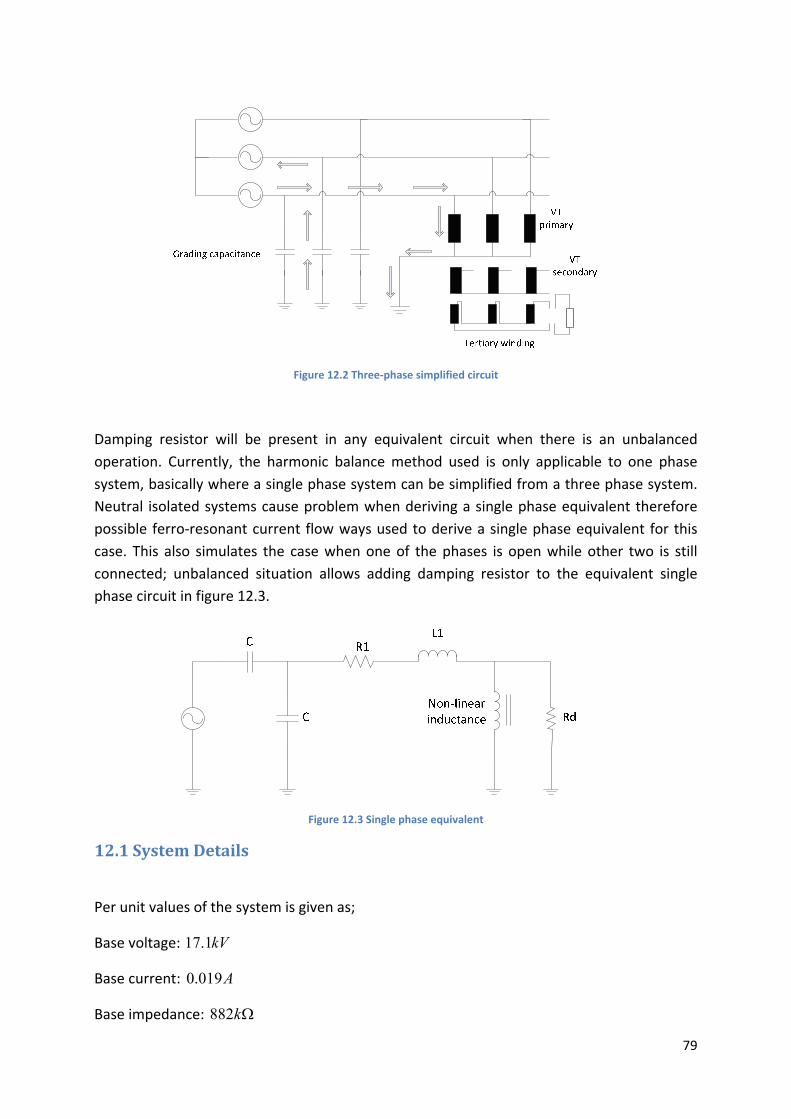
79
Figure 12.2 Three‐phase simplified circuit
Damping resistor will be present in any equivalent circuit when there is an unbalanced
operation. Currently, the harmonic balance method used is only applicable to one phase
system, basically where a single phase system can be simplified from a three phase system.
Neutral isolated systems cause problem when deriving a single phase equivalent therefore
possible ferro‐resonant current flow ways used to derive a single phase equivalent for this
case. This also simulates the case when one of the phases is open while other two is still
connected; unbalanced situation allows adding damping resistor to the equivalent single
phase circuit in figure 12.3.
Figure 12.3 Single phase equivalent
12.1 SystemDetails
Per unit values of the system is given as;
Base voltage: 17.1kV
Base current: 0.019A
Base impedance: 882k
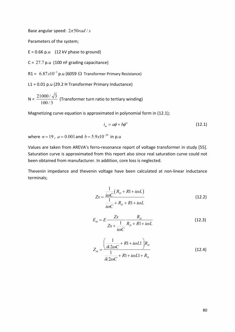
80
Base angular speed: 2 50 /rad s
Parameters of the system;
E = 0.66 p.u (12 kV phase to ground)
C = 27.7 p.u (100 nF grading capacitance)
R1 = 36.87 10x p.u (6059 Transformer Primary Resistance)
L1 = 0.01 p.u (29.2 H Transformer Primary Inductance)
N = 21000 / 3
100 / 3 (Transformer turn ratio to tertiary winding)
Magnetizing curve equation is approximated in polynomial form in (12.1);
nmi a b (12.1)
where 19n , 0.001a and 395.9 10b x in p.u
Values are taken from AREVA’s ferro‐resonance report of voltage transformer in study [55].
Saturation curve is approximated from this report also since real saturation curve could not
been obtained from manufacturer. In addition, core loss is neglected.
Thevenin impedance and thevenin voltage have been calculated at non‐linear inductance
terminals;
1
1
11
D
D
R R i Li CZx
R R i Li C
(12.2)
1 1
Dth
D
RZxE E
R R i LZxi C
(12.3)
11 1
21
1 12
D
th
D
R i L Rik C
ZR i L R
ik C
(12.4)
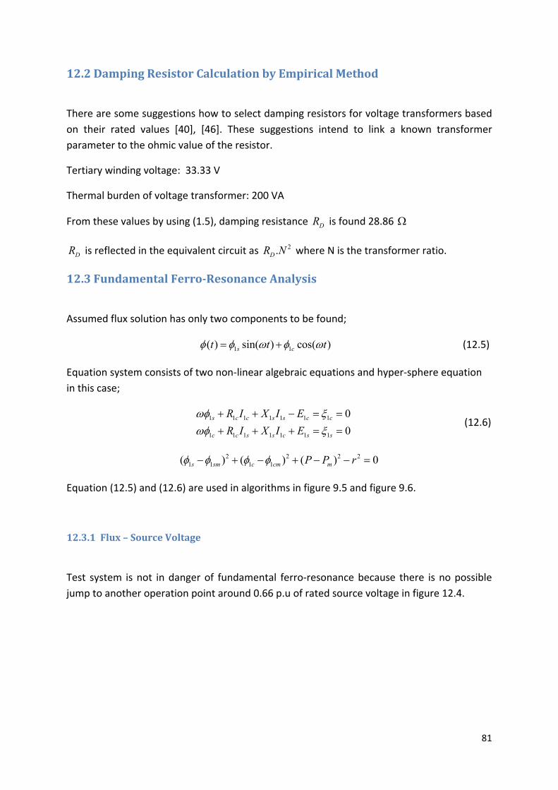
81
12.2 DampingResistorCalculationbyEmpiricalMethod
There are some suggestions how to select damping resistors for voltage transformers based
on their rated values [40], [46]. These suggestions intend to link a known transformer
parameter to the ohmic value of the resistor.
Tertiary winding voltage: 33.33 V
Thermal burden of voltage transformer: 200 VA
From these values by using (1.5), damping resistance DR is found 28.86
DR is reflected in the equivalent circuit as 2.DR N where N is the transformer ratio.
12.3 FundamentalFerro‐ResonanceAnalysis
Assumed flux solution has only two components to be found;
1 1( ) sin( ) cos( )s ct t t (12.5)
Equation system consists of two non‐linear algebraic equations and hyper‐sphere equation
in this case;
1 1 1 1 1 1 1
1 1 1 1 1 1 1
0
0s c c s s c c
c c s s c s s
R I X I E
R I X I E
(12.6)
2 2 2 21 1 1 1( ) ( ) ( ) 0s sm c cm mP P r
Equation (12.5) and (12.6) are used in algorithms in figure 9.5 and figure 9.6.
12.3.1 Flux–SourceVoltage
Test system is not in danger of fundamental ferro‐resonance because there is no possible
jump to another operation point around 0.66 p.u of rated source voltage in figure 12.4.
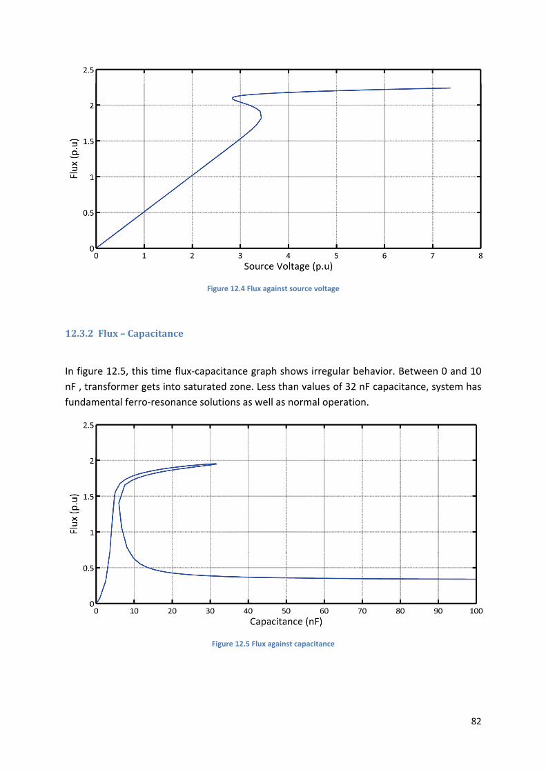
82
Figure 12.4 Flux against source voltage
12.3.2 Flux–Capacitance
In figure 12.5, this time flux‐capacitance graph shows irregular behavior. Between 0 and 10
nF , transformer gets into saturated zone. Less than values of 32 nF capacitance, system has
fundamental ferro‐resonance solutions as well as normal operation.
Figure 12.5 Flux against capacitance
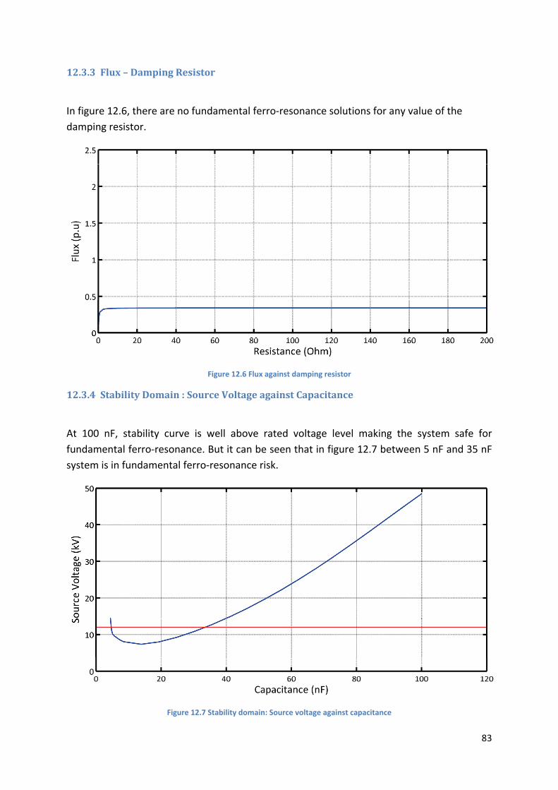
83
12.3.3 Flux–DampingResistor
In figure 12.6, there are no fundamental ferro‐resonance solutions for any value of the
damping resistor.
Figure 12.6 Flux against damping resistor
12.3.4 StabilityDomain:SourceVoltageagainstCapacitance
At 100 nF, stability curve is well above rated voltage level making the system safe for
fundamental ferro‐resonance. But it can be seen that in figure 12.7 between 5 nF and 35 nF
system is in fundamental ferro‐resonance risk.
Figure 12.7 Stability domain: Source voltage against capacitance
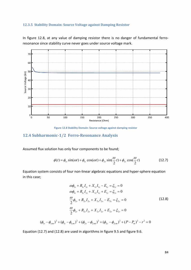
84
12.3.5 StabilityDomain:SourceVoltageagainstDampingResistor
In figure 12.8, at any value of damping resistor there is no danger of fundamental ferro‐
resonance since stability curve never goes under source voltage mark.
Figure 12.8 Stability Domain: Source voltage against damping resistor
12.4 Subharmonic‐1/2Ferro‐ResonanceAnalysis
Assumed flux solution has only four components to be found;
1 1 2 2( ) sin( ) cos( ) sin( ) cos( )2 2s c s ct t t t t (12.7)
Equation system consists of four non‐linear algebraic equations and hyper‐sphere equation
in this case;
1 1 1 1 1 1 1
1 1 1 1 1 1 1
2 2 2 2 2 2 2
2 2 2 2 2 2 2
0
0
02
02
s c c s s c c
c c s s c s s
s c c s s c c
c c s s c s s
R I X I E
R I X I E
R I X I E
R I X I E
(12.8)
2 2 2 2 2 21 1 1 1 2 2 2 2( ) ( ) ( ) ( ) ( ) 0s sm c cm s sm c cm mP P r
Equation (12.7) and (12.8) are used in algorithms in figure 9.5 and figure 9.6.
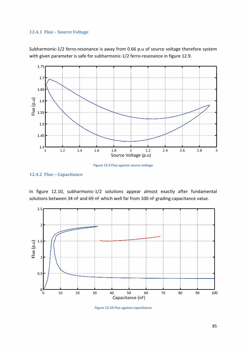
85
12.4.1 Flux–SourceVoltage
Subharmonic‐1/2 ferro‐resonance is away from 0.66 p.u of source voltage therefore system
with given parameter is safe for subharmonic‐1/2 ferro‐resonance in figure 12.9.
Figure 12.9 Flux against source voltage
12.4.2 Flux–Capacitance
In figure 12.10, subharmonic‐1/2 solutions appear almost exactly after fundamental
solutions between 34 nF and 69 nF which well far from 100 nF grading capacitance value.
Figure 12.10 Flux against capacitance
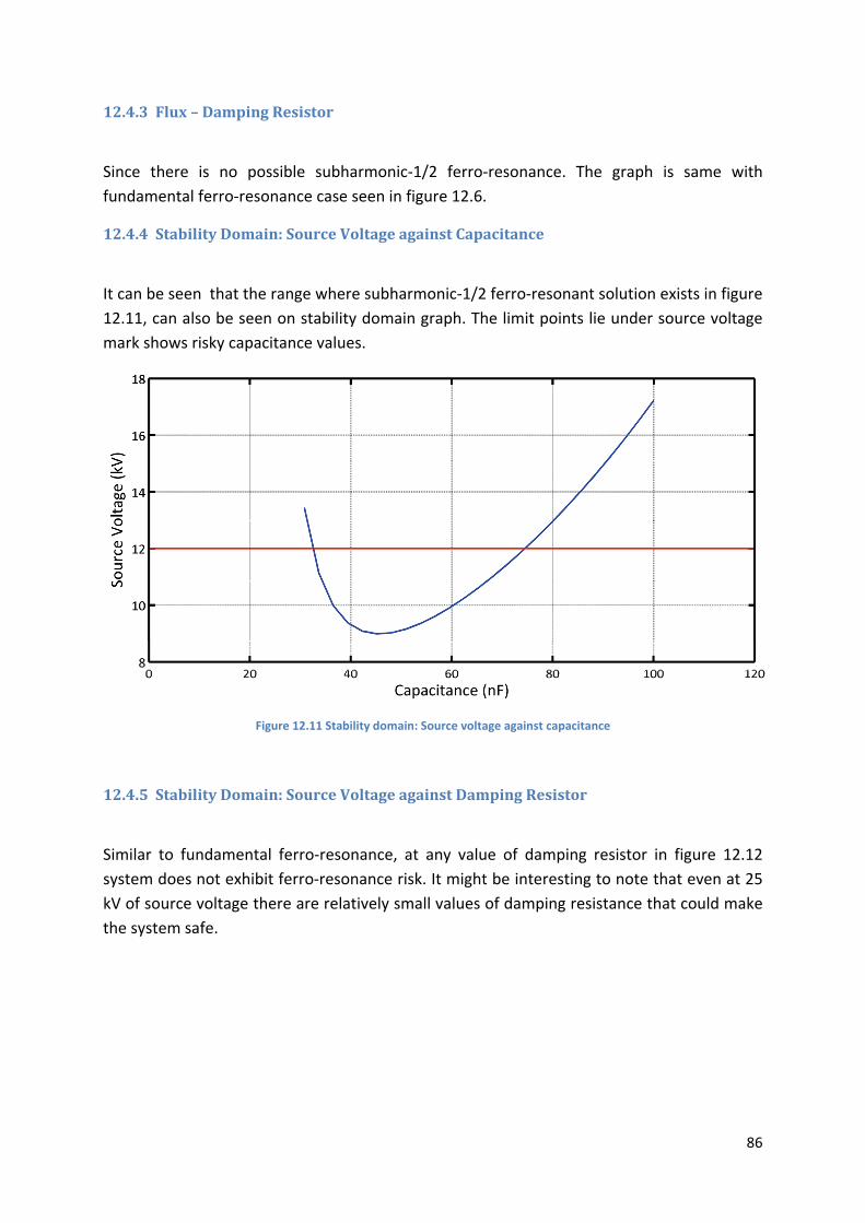
86
12.4.3 Flux–DampingResistor
Since there is no possible subharmonic‐1/2 ferro‐resonance. The graph is same with
fundamental ferro‐resonance case seen in figure 12.6.
12.4.4 StabilityDomain:SourceVoltageagainstCapacitance
It can be seen that the range where subharmonic‐1/2 ferro‐resonant solution exists in figure
12.11, can also be seen on stability domain graph. The limit points lie under source voltage
mark shows risky capacitance values.
Figure 12.11 Stability domain: Source voltage against capacitance
12.4.5 StabilityDomain:SourceVoltageagainstDampingResistor
Similar to fundamental ferro‐resonance, at any value of damping resistor in figure 12.12
system does not exhibit ferro‐resonance risk. It might be interesting to note that even at 25
kV of source voltage there are relatively small values of damping resistance that could make
the system safe.
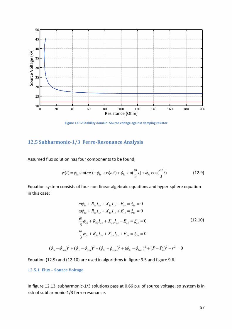
87
Figure 12.12 Stability domain: Source voltage against damping resistor
12.5 Subharmonic‐1/3Ferro‐ResonanceAnalysis
Assumed flux solution has four components to be found;
1 1 3 3( ) sin( ) cos( ) sin( ) cos( )3 3s c s ct t t t t (12.9)
Equation system consists of four non‐linear algebraic equations and hyper‐sphere equation
in this case;
1 1 1 1 1 1 1
1 1 1 1 1 1 1
3 3 3 3 3 3 3
3 3 3 3 3 3 3
0
0
03
03
s c c s s c c
c c s s c s s
s c c s s c c
c c s s c s s
R I X I E
R I X I E
R I X I E
R I X I E
(12.10)
2 2 2 2 2 21 1 1 1 3 3 3 3( ) ( ) ( ) ( ) ( ) 0s sm c cm s sm c cm mP P r
Equation (12.9) and (12.10) are used in algorithms in figure 9.5 and figure 9.6.
12.5.1 Flux–SourceVoltage
In figure 12.13, subharmonic‐1/3 solutions pass at 0.66 p.u of source voltage, so system is in
risk of subharmonic‐1/3 ferro‐resonance.
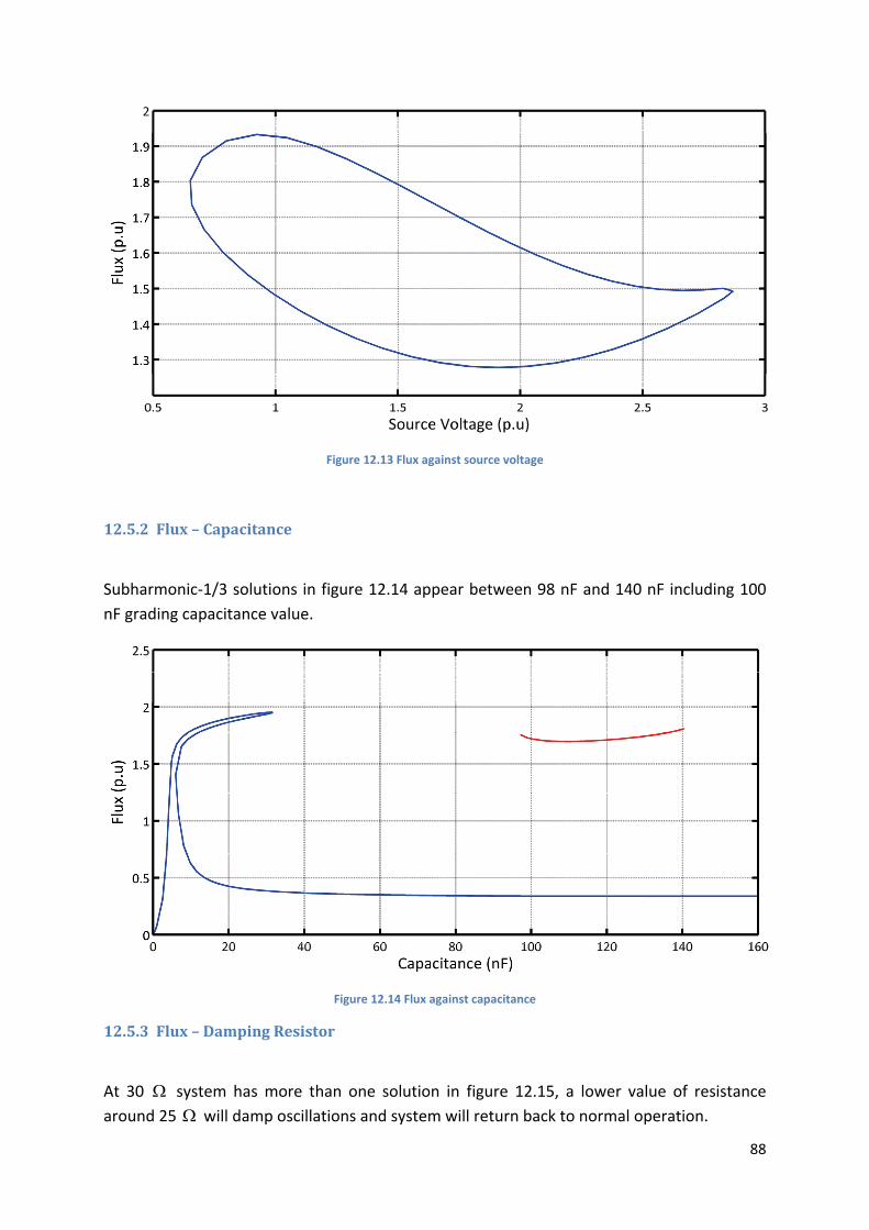
88
Figure 12.13 Flux against source voltage
12.5.2 Flux–Capacitance
Subharmonic‐1/3 solutions in figure 12.14 appear between 98 nF and 140 nF including 100
nF grading capacitance value.
Figure 12.14 Flux against capacitance
12.5.3 Flux–DampingResistor
At 30 system has more than one solution in figure 12.15, a lower value of resistance
around 25 will damp oscillations and system will return back to normal operation.
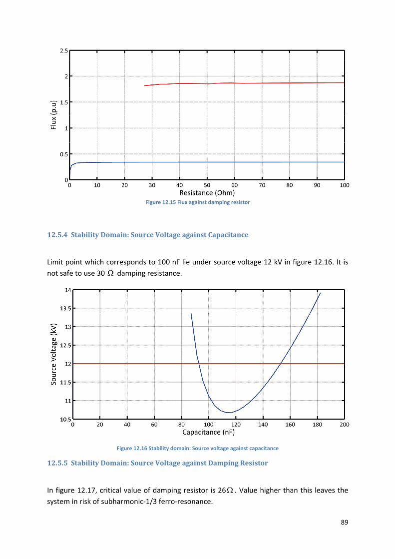
89
Figure 12.15 Flux against damping resistor
12.5.4 StabilityDomain:SourceVoltageagainstCapacitance
Limit point which corresponds to 100 nF lie under source voltage 12 kV in figure 12.16. It is
not safe to use 30 damping resistance.
Figure 12.16 Stability domain: Source voltage against capacitance
12.5.5 StabilityDomain:SourceVoltageagainstDampingResistor
In figure 12.17, critical value of damping resistor is 26 . Value higher than this leaves the
system in risk of subharmonic‐1/3 ferro‐resonance.
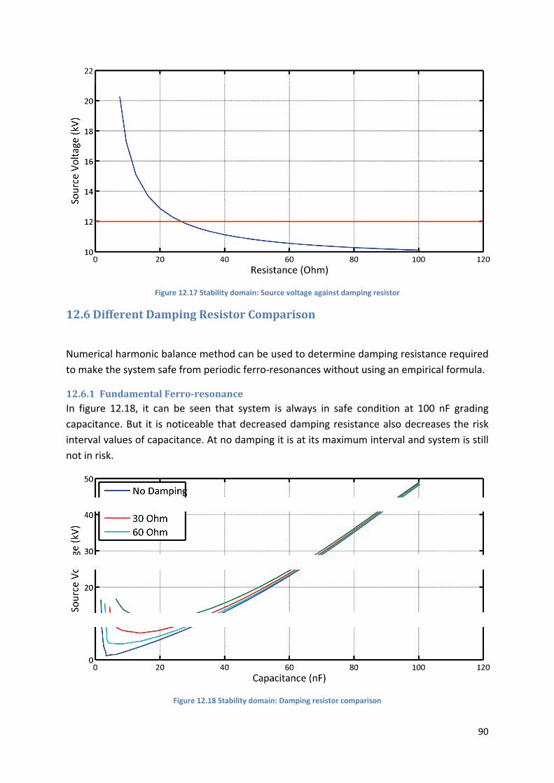
90
Figure 12.17 Stability domain: Source voltage against damping resistor
12.6 DifferentDampingResistorComparison
Numerical harmonic balance method can be used to determine damping resistance required
to make the system safe from periodic ferro‐resonances without using an empirical formula.
12.6.1 FundamentalFerro‐resonanceIn figure 12.18, it can be seen that system is always in safe condition at 100 nF grading
capacitance. But it is noticeable that decreased damping resistance also decreases the risk
interval values of capacitance. At no damping it is at its maximum interval and system is still
not in risk.
Figure 12.18 Stability domain: Damping resistor comparison
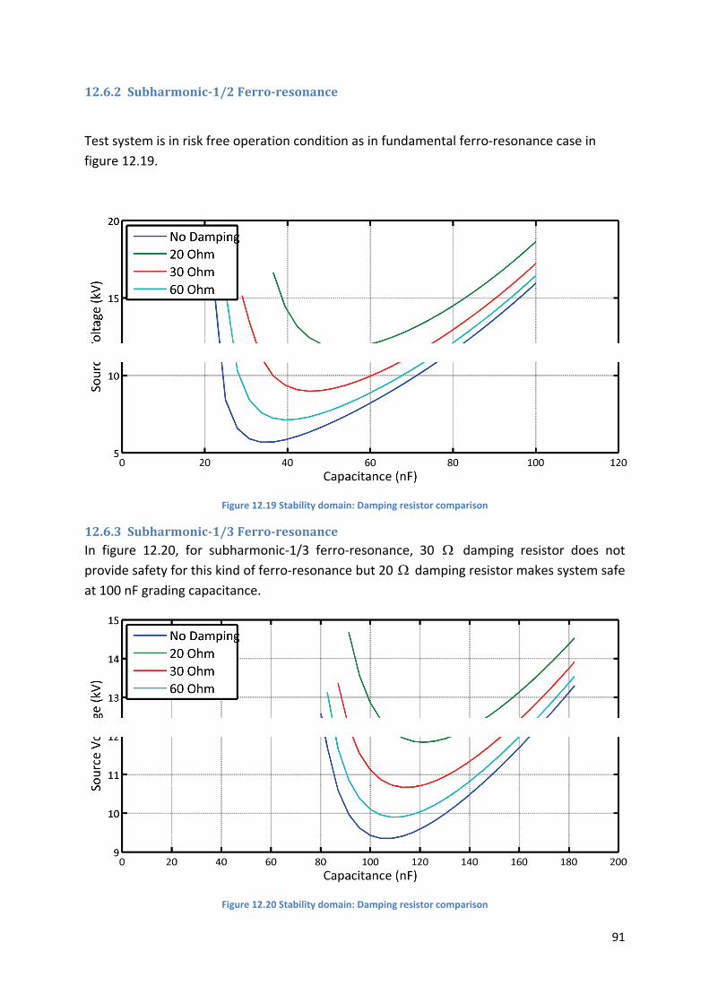
91
12.6.2 Subharmonic‐1/2Ferro‐resonance
Test system is in risk free operation condition as in fundamental ferro‐resonance case in
figure 12.19.
Figure 12.19 Stability domain: Damping resistor comparison
12.6.3 Subharmonic‐1/3Ferro‐resonanceIn figure 12.20, for subharmonic‐1/3 ferro‐resonance, 30 damping resistor does not
provide safety for this kind of ferro‐resonance but 20 damping resistor makes system safe
at 100 nF grading capacitance.
Figure 12.20 Stability domain: Damping resistor comparison
92
12.6.4 Remarks
Empirical calculation of the resistance did not provide safety from subharmonic‐1/3 if it is
considered 30 , but numerical harmonic balance method showed that 20 damping
resistor will be needed. It does seem that empirical formula suggested might not be the best
way to determine damping resistor, and it will be hard to support the way of its calculation.
Harmonic balance method can show that if there is a danger of ferro‐resonance or not. It can
be shown that selection of resistor really provides a protection.
13 CurrentIssueswithHarmonicBalanceStudyofFerro‐resonance
1 – Unfortunately the algorithm for numerical harmonic balance method is not fully
automated. Hyper‐sphere radius, P and tolerance for MATHCAD solver needs to be
adjusted manually each time when there is a convergence problem or if the solver is having
hard time to turn limit points. It may take some to find correct parameters. Pseudo‐arc
length continuation method has been tried but due to mathematical problem of defining
tangent vector at limit point, turning around limit points could not been achieved.
2 – MATHCAD seems to be very slow when calculating more Fourier components. The
advantage of MATHCAD is that equation system solvers are already built‐in functions. A
basic Newton‐Rhapson method coded manually may not provide enough convergence
capabilities therefore create some other mathematical problems to solve equations.
3 – Magnetization curve as known as real saturation curve is needed from the manufacturer
of transformer. During the time of internship, it could not be obtained and an approximation
had to be used. By keeping in mind that parameters are very important on solution regimes,
equivalent circuit and its parameters should be known correctly.
4 ‐ Finding subharmonic solutions is not easy because they do not have a trivial solution like
fundamental does (0,0) point. So by adjusting initial guess values to the solver, a single point
should be found on the subharmonic isolate to start continuation method. That single point
is found by trial and error. Since p.u values are used, initial guess value range is around ‐2
and 2. But still it might take time to find them.
5 – Deciding on components of the assumed flux solution is not clear in literature. Effect of
components on each other should be analyzed in another study. There is also no comparison
between occurrence of different type of ferro‐resonances, this study included fundamental
and subharmonics but information about which ferro‐resonance would likely to happen
could not be given.
6 ‐ Determining the equivalent circuit for neutral‐isolated systems is controversial. To use
this method explained here, it is needed to work with a single phase equivalent. But it is said
93
that neutral‐isolated systems cannot be simplified into one‐phase equivalent [44]. The
nonlinearity between flux and magnetizing current does not allow using linear
transformation to use zero‐sequence circuit to analyze damping effect of damping
resistance. Studying “forced” unbalanced system may not be correct. To apply harmonic
balance to three‐phase circuits, mutual impedances should be found between phases which
gets very complicated since numbers of unknown get tripled.
7 – Finding real cases to test numerical harmonic balance method on ferro‐resonance is hard
to find. Especially saturation curves are not given most of the time causing use of harmonic
balance meaningless in that case.
14 SummaryandConclusion
Ferro‐resonance even though it is not very common is a problem to power systems. It has
dangerous consequences like stable over voltages and over currents. Risky configurations
are mentioned and prevention of ferro‐resonance is discussed. Time‐domain simulations are
not enough to study for these kinds of phenomena since ferro‐resonance may happen or
may not happen depending of circuit parameters and initial conditions prior to any event in
the system. Due to this problem of time‐domain analysis, direct calculation of steady states
is done with harmonic balance method. Two methods of harmonic balance have been
discussed namely analytical and numerical harmonic balance method. Numerical harmonic
balance method showed advantages on application and study on different kinds of ferro‐
resonances. In order to deal with continuation problem while drawing two parameter
graphs, a hyper‐sphere method is applied. Two examples from literature have been
extensively analyzed with harmonic balance and also Alstom’s test system went under the
same study with other cases. Stability domain of different kind of ferro‐resonances provides
large insight to the ferro‐resonance phenomena. By changing any kind of parameter in the
system it can be observed if that change put the system in or out of ferro‐resonance danger.
This feature is used to determine damping resistance to damp ferro‐resonant oscillations
and do not allow them to become steady‐state. Without using empirical method to calculate
resistance, decision on damping resistor by harmonic balance method is more scientifically
backed up. There are still problems with the method has been applied and those were
discussed in chapter 13.
This study considers that static damping is used for prevention of ferro‐resonance in voltage
transformers. Due to problems in this method, dynamical damping may be an option for
power system designers, it would automatically control itself for any kind of oscillation and
adjust itself to damp oscillations. Then it will not be necessary to think about which kind of
ferro‐resonance should be studied and for which kind of ferro‐resonance the damping
resistor should be calculated. Harmonic balance study showed that different ferro‐resonance
types needs different damping resistance values. As the parallel losses increased by lowering
94
the damping resistance, it is possible to provide protection from other types of ferro‐
resonance if it is not provided before. Lowering resistance value might have some thermal
restrictions for voltage transformers but that study is not done here.
Existence zone for fundamental and subharmonic ferro‐resonances are very close so even if
the real possibility of occurrence is not known, it is better not to leave it to chance and
provide a damping resistance that would make the system risk free of ferro‐resonance. In
Alstom’s test system, empirical method to calculate damping resistance provided safety for
fundamental and subharmonic‐1/2 ferro‐resonance but not for subharmonic‐1/3 after it has
been checked with harmonic balance method. Not only for damping resistance but values of
the grading capacitance value can be calculated with this way also if it is needed. The power
of harmonic balance method comes from its flexibility of use.
Correct selection of damping resistor will prevent ferro‐resonance therefore it can avoid
unpredictable accidents that may happen in power systems and power plant networks. It
contributes to general safety of power systems and even safety for human life.
For future studies, algorithm proposed can be tried with another continuation method such
as pseudo‐arc length method and solve computation problems at limit points. MATHCAD
seems to be slow on non‐linear equation solving when it comes to calculate many Fourier
components. An algorithm can be coded from scratch in FORTRAN or MATLAB but it is not
sure it would drastically reduce computation time. Because of this problem studies done in
this project do not contain many Fourier components that would make solutions more
accurate.
It is known that voltage transformers have non‐linear core loss, and during saturation losses
are increased. This could have effect on calculations of ferro‐resonance. By adopting a
proper model for core loss, calculations will present more accurate real life cases. Increased
losses help damping of the system so calculations done without including the extra losses by
non‐linear core loss would be in safe design side.
Three‐phase analysis can be done for isolated neutral systems. In this project one‐phase
equivalents are used because three‐phase analysis turned out to be has not been done
therefore no information could have been found on this matter for guidance.
95
15 References1‐ P. Boucherot, "Éxistence de Deux Régimes en Ferrorésonance", Rev. Gen. de L’Élec.,
vol. 8, no. 24, 1920
2‐ Glenn W. Swift, “An Analytical Approach to Ferroresonance”, IEEE Transactions, vol.
pas‐88, no. 1,1969
3‐ J. Bethenod, "Sur le Transformateur à Résonance", L'Éclairage Électrique, vol. 53,
1907
4‐ C. Hayashi, Nonlinear Oscillations in Physical Systems, Princeton University Press,
Princeton‐New Jersey, 1985.
5‐ David A. N. Jacobson, Peter W. Lehn and Robert W. Menzies, “Stability Domain
Calculation of Period‐1 Ferroresonance in a Nonlinear Resonant Circuit”, IEEE
Transactions on Power Delivery, vol. 17, no. 3, July 2002.
6‐ A. Germond, “Computation of Ferroresonant Overvoltages in Actual Power Systems
by Galerkin's Method”, Proceedings of IEEE PICA, New Orleans, 1975.
7‐ P. Bornard, V. Collet Billion and C. Kieny, “Protection of EHV Power Systems Against
Ferroresonance”, 1990 CIGRE, paper 34‐103, pp. 1‐8, 1990.
8‐ M. Moradi and A. Gholami, “Initial Condition Effect on Ferroresonance Behavior in a
Nonlinear Circuit”, Proceedings of International Power System Conference, 98‐E‐HVS‐
799, Iran, 2007.
9‐ Zhu Xukai, Yang Yihan, Lian Hongbo and Tan Weipu, “Study on Ferroresonance due to
Electromagnetic PT in Ungrounded Neutral System”, Proceedings of Power System
Technology – POWERCON, Singapore, 21‐24 November 2004.
10‐ Y.C Kang et al., “Analytical Analysis of PT Ferroresonance in the Transient‐State”,
Proceedings of 10th IET International Conference, Manchester, 2010.
11‐ S. Mozaffari, M. Sameti and A.C. Soudack, “Effect of initial conditions on chaotic
ferroresonance in power transformers”, IEE Proc.‐Gener. Transm. Distrib., vol. 144,
no. 5, September 1997.
12‐ Madhab Roy and Chinmay Kanti Roy, “A Study on Ferroresonance with a varying
Initial Conditions using a Nonlinear Model of Transformer”, Proceedings of Third
International Conference on Power Systems, no. 213, India, 2009.
13‐ Afshin Rezaei‐Zare and Reza Iravani, “Impacts of Various Representations of Core
Saturation Curve on Ferroresonance Behavior of Transformer”, Proceedings of
International Conference on Power Systems Transients IPST, Japan, June 3‐6 2009.
14‐ M. Moradi and A. Gholami, “A Harmonic Balance Based Stability Domain Analysis of
Period‐1 Ferroresonance”, Proceedings of 25th International Power System
Conference, 10‐E‐TRN‐1839, Iran, 2010.
15‐ T. Tran‐Quoc and L. Pierrat, “An Efficient Non‐Linear Transformer Model and Its
Application to Ferroresonance Study”, IEEE Transactions on Magnetics, vol. 31, no. 3,
May 1995.
16‐ Afshin Rezaei‐Zare et al., “An Accurate Hysteresis Model for Ferroresonance Analysis
of a Transformer”, IEEE Transactions on Power Delivery, vol. 23, no.3, July 2008.
96
17‐ P.S. Moses and M.A.S Masoum, “Sensitivity of ferroresonance simulations to model
parameters and initial conditions”, Proceedings of Universities Power Engineering
Conference (AUPEC), pp. 1‐6, New Zealand, 5‐8 December 2010.
18‐ P. Sakarung, T. Bunyagul and S. Chatratana, “Investigation and Mitigation of
Overvoltage Due to Ferroresonance in the Distribution Network”, Journal of Electrical
Engineering and Technology, vol. 2, no. 3, pp. 300‐305, 2007
19‐ Yunge Li, Wei Shi, Rui Qin and Jilin Yang, “A Systematical Method for Suppressing
Ferroresonance at Neutral‐Grounded Substations”, IEEE Transactions on Power
Delivery, vol. 18, no.3, July 2003.
20‐ L. X. Zhou and Z. D. Yin, “Research on PT Ferromagnetic Resonance and the
Controllable Damping”, Proceedings of IEEE Power Tech Conference, pp. 413‐418,
Lausanne, 1‐5 July 2007.
21‐ Hamid Radmanesh and Mehrdad Rostami, “Effect of Circuit Breaker Shunt Resistance
on Chaotic Ferroresonance in Voltage Transformer”, Advances in Electrical and
Computer Engineering, vol. 10, no. 3, 2010.
22‐ Marneni Lakshmi Prasad, Madhab Roy and Chinmay Kanti Roy, “Analysis of
Ferroresonant Oscillations in a Nonlinear Circuit”, Proceedings of IEEE Region 10
Colloquium and the Third ICIIS, India, 8‐10 December 2008.
23‐ P.S. Bodger, G.D. Irwin, D.A. Woodford and A.M. Gole, “ Bifurcation route to chaos
for a ferroresonant circuit using an electromagnetic transients program”, IEE Proc.‐
Gener Transm. Distrib., vol.143, no. 3, May 1996.
24‐ B.A. Mork and D.L. Stuehm, “Application of nonlinear dynamics and chaos to
ferroresonance in distribution systems”, IEEE Transactions on Power Delivery, vol. 9,
no. 2, April 1994.
25‐ M. Stosur, W. Piasecki, M. Florkowski and M. Fulczyk, “ATP/EMTP Study of
Ferroresonance Involving HV Inductive VT and Circuit Breaker Capacitance”, Electrical
Power Quality and Utilization Journal, vol. 14, no. 2, 2008.
26‐ A.C. Soudack and S. Mozaffari, “Chaos in a Power Transformer”, Proceedings of
Control of Oscillations and Chaos, vol. 1, Russia, 1997.
27‐ A.E.A. Araujo, A.C. Soudack and J.R. Marti, “Ferroresonance in power systems:
chaotic behavior”, IEE Proceedings‐C, vol. 140, no. 3, May 1993.
28‐ Z. Emin, B.A.T. Al Zahawi, D.W. Auckland and Y.K Tong, “Ferroresonance in
electromagnetic voltage transformers: A study based on nonlinear dynamics”, IEE
Proc.‐Gener. Transm. Distrib., vol. 144, no. 4, July 1997.
29‐ Zhang Bo and Lu Tiecheng, “Application of Nonlinear Dynamic on Ferroresonance in
Power System”, Proceedings of Asia‐Pacific Power and Energy Engineering
Conference, pp. 1‐4, Wuhan China, 27‐31 March 2009.
30‐ P. Sakarung and S. Chatratana, “Application of PSCAD/EMTDC and Chaos Theory to
Power System Ferroresonance Analysis”, Proceedings of International Conference on
Power Systems Transients (IPST), no. 227, Montreal, Canada, 19‐23 June 2005.
97
31‐ J.R Marti and A.C. Soudack, “Ferroresonance in power systems: Fundamental
solutions”, IEE Proceedings‐C, vol. 138, no. 4, July 1991.
32‐ A. Bardhi, P. Cipo and M. Braneshi, “Study of a ferroresonant circuit using analytic
harmonic balance, numerical integration of nonlinear ODE and experimental
methods”, Proceedings of 14th International Power Electronics and Motion Control
Conference, pp. 8‐12, Wuhan, China, 6‐8 September 2010.
33‐ Maher S. Maklad and Moustafa M. Fahmy, “An analytical investigation of a
Ferroresonant Circuit”, IEEE Transactions on Magnetics, vol. 16, no. 2, March 1980.
34‐ C. Kieny, “Application of the bifurcation theory in studying and understanding the
global behavior of a ferroresonant electric power circuit”, IEEE Transactions on Power
Delivery, vol. 6, no. 2, April 1991.
35‐ C. Kieny and A. Sbai, “Ferroresonance study using Galerkin Method with Pseudo‐
Arclength Continuation Method”, IEEE Transactions on Power Delivery, vol. 6, no. 4,
October 1991.
36‐ Fathi Ben Amar and Rachid Dhifaoui, “Bifurcation Lines Calculations of Period‐1
Ferroresonance”, Proceedings of the 6th WSAES International Conference on Power
Systems, Lisbon, Portugal, 22‐24 September 2006.
37‐ Fathi Ben Amar and Rachid Dhifaoui, “Study of the periodic ferroresonance in the
electrical power networks by bifurcation diagrams”, Electrical Power and Energy
Systems, vol. 33, pp. 61‐85, 2011.
38‐ T. Van Craenenbroeck, D. Van Dommelen, J. Driesen and R. Belmans, “Application of
the harmonic balance method to study ferroresonance in voltage transformers”,
Proceedings of 11th International Symposium on High Voltage Engineering, no. 467,
London, 1999.
39‐ T. Van Craenenbroeck, D. Van Dommelen, N. Janssens and F. Van De Meulebroeke,
“Stability Analysis of Ferroresonant Oscillations in Networks with Isolated Neutral”,
Proceedings of First IEEE International Caracas Conference on Devices, Circuits and
Systems, pp. 41‐45, 12‐14 December 1995.
40‐ T. Van Craenenbroeck, D. Van Dommelen and N. Janssens, “Damping Circuit Design
for Ferroresonance in Floating Power Systems”, European Transactions on Electrical
Power, vol. 10, no. 3, May/June 2000.
41‐ T. Van Craenenbroeck, W. Michiels, D. Van Dommelen and K. Lust, “Bifurcation
Analysis of Three‐Phase Ferroresonant Oscillations in Ungrounded Power Systems”,
IEEE Transactions on Power Delivery, vol. 14, no. 2, April 1999.
42‐ C. Stuckens, P.A. Monfils, N. Janssens, T. Van Craenenbroeck and D. Van Dommelen, “
Risk of Ferroresonance in Isolated Neutral Networks and Remedies”, Proceedings of
IEEE Conference, CIRED Issue No. 438, Birmingham, 2‐5 June 1997.
43‐ C. Stuckens, P.A. Monfils, N. Janssens, T. Van Craenenbroeck and D. Van Dommelen,
“Harmonic balance based bifurcation analysis of three‐phase ferroresonance with full
scale experimental validation”, Proceedings of Transmission and Distribution
Conference, vol. 2, New Orleans, Los Angeles, 1999.
98
44‐ T. Van Craenenbroeck, D. Van Dommelen, N. Janssens and F. Van De Meulebroeke,
“Direct Calculation of the Stability Domains of Three‐Phase Ferro‐resonance in
Isolated Neutral Networks with Grounded‐Neutral Voltage Transformers”, IEEE
Transactions on Power Delivery, vol. 11, no. 3, July 1996.
45‐ T. Van Craenenbroeck, D. Van Dommelen and R. Belmans, “Comparison of Three
Methods to Study Ferro‐resonance in Voltage Transformers”, Electrical Engineering
Research Report, vol. 9, July 2000.
46‐ P. Ferraci, “Ferroresonance”, Groupe Schneider: Cahier technique no. 190, pp. 1‐28,
March 1998. [ Available at www.schneiderelectric.com/en/pdf//ect190.pdf]
47‐ M. Val Escudero, I. Dudurych, and M.A. Redfern, "Characterization of ferroresonant
modes in HV substation with CB grading capacitors", Electric Power Systems
Research, vol. 77, pp. 1506‐1513, 2007.
48‐ D.A.N. Jacobson, D.R. Swatek and R.W. Mazur, “Mitigating Potential Transformer
Ferroresonance in a 230 kV Converter Station”, Proceedings of IEEE Transmission and
Distribution Conference, pp. 269‐275, Los Angeles, 1996.
49‐ K. Pattanapakdee and C. Banmongkol, “Failure of Rise Pole Arrester Due to Station
Service Transformer Ferroresonance”, Proceedings of International Conference on
Power Systems Transients, Lyon, 4‐7 June 2007.
50‐ “Technical Bulletin – 004a Ferroresonance”, Cadick Corporation, 29 May 2002. [
Available at www.cadickcorp.com/download/TB004a_Ferroresonance.pdf ]
51‐ S. El‐Rabaie, Vincent F. Fusco and Carson Stewart, “Harmonic Balance Evaluation of
Nonlinear Microwave Circuits – A Tutorial Approach”, IEEE Transactions on
Education, vol. 31, no. 3, August 1988.
52‐ Rowan J. Gilmore and Michael B. Steer, “Nonlinear Circuit Analysis Using the Method
of Harmonic Balance – A Review of the Art. Part I. Introductory Concepts”,
International Journal of Microwave and Millimeter‐Wave Computer‐Aided
Engineering, vol. 1, no. 1, 1991.
53‐ Avrum C. Soudack, “A Generalized Ritz Method and Its Application to Certain
Nonlinear System Problems”, IEEE Transactions on Education, vol. 9, no. 1, March
1966.
54‐ Kiyotaka Yamamura, “Simple Algorithms for Tracing Solution Curves”, IEEE
Transactions Circuit and Systems I: Fundamental Theory and Applications, vol. 40, no.
8, pp. 537‐541, August 1993.
55‐ P.A Monfils, “Ferro resonance risk calculation report on VT’s installed on Combigolfe
generator CB’s”, Internal Report, AREVA, March 2010.
56‐ IEC 71 International Standard , “Insulation Co‐ordination”, 1996.


