INPE-8981-TDI/812/B PARAMETERS IDENTIFICATION AND FAILURE DETECTION APPLIED TO SPACE ROBOTIC MANIPULATORS Adenilson Roberto da Silva Dissertation in Space Engineering and Technology in partial fulfillment of the requirements for Doctor degree, supervised by Dr. Luiz Carlos Gadelha de Souza and Dr. Bernd Schäfer, approved in november the 11 th , 2001. INPE São José dos Campos 2002
Transcript
INPE-8981-TDI/812/B
PARAMETERS IDENTIFICATION AND FAILURE DETECTION APPLIED TO SPACE ROBOTIC MANIPULATORS
Adenilson Roberto da Silva
Dissertation in Space Engineering and Technology in partial fulfillment of the requirements for Doctor degree, supervised by Dr. Luiz Carlos Gadelha de Souza and
Dr. Bernd Schäfer, approved in november the 11th , 2001.
INPE São José dos Campos
2002
629.7.062.2 SILVA, A. R. Parameters identification and failure detection applied to robotic maniputators / A. R. Silva. – São José dos Campos: INPE, 2001. 183p. – (INPE-8981-TDI/812/B). 1.Parameters identification. 2.System identification. 3.Robot dynamic. 4.Nonlinear systems. 5.Least square method. 6.Robots. 7.Fault detection. I.Título.
To everyone, which have shared with me the happiness of this victory,
I dedicate.
ACKNOWLEDGEMENTS
My sincere appreciation goes to my advisors Dr. Luiz C. G. de Souza and Dr. Bernd
Schäfer. Their challenging questions, insightful comments and stimulating discussions
always kept me thinking and learning.
I wish to express my gratitude to all of my doctorate professors, especially Drs. Marcelo
Lopes, Roberto Lopes for their incentive and fruitful comments during my research at
INPE. They have taught not technical lessons, but also how to be a critic and a minute
researcher.
I would like to thank all of examination group for their comments and suggestions that
have improved and enriched my work
My appreciation also goes to Prof. Luis S. Goes from ITA. His comments has always
improved my thought and helped me to solve problems during my research.
I thank DLR for propitiate an excellent environment and support during my stay in
Germany. My stay at DLR (and in Germany) was made much more enjoyable by the
company of various staff members. I wish also to express my gratitude to Rainer Krenn
for his help and friendship during all my stay. The pizza (after the work), the barbecue
and the mountain trekking will be always a fond memory. At this point, I wish to thank
Dr. Bernd Schäfer for his help and friendship. I am quite sure that may stay at Germany
would not be completely enjoyable without his friendship.
My appreciation goes to all of my colleagues for their friendship and support. My
special thanks to Evandro M. Rocco (who has shared a office for four years), Walkiria
Schulz, Ana P. Chiaridia, Cristina Tobler, Francisco Carvalho for their support and
friendship.
I express my gratitude also to Luiz R. R. Faria for his incentive in the beginning of my
education and also along my entire career.
I wish to thank my parents, Josué and Antonia, all my sisters, brothers, nephew and
nieces, at last all of my family (it will take to long to write down all names) for their
love and support throughout my life. I wish also to thank my girlfriend Keli for her love
and tolerance during my student lifestyle.
ABSTRACT
Physical parameters identification is useful in many applications, especially in aerospace and robotics fields. Aerospace and robotics system analysis normally requires accurate physical system models for control. On the other hand, the identification of physical parameters, besides the normal identification requirements (system excitation, for instance), involves several tasks: mathematical modeling and algorithm selection for instance. In this thesis, a detailed modeling of a robotic joint has been presented. The models are derived in an increasing degree of complexity (which means that, in theory, the mathematical representation is approaching to the real system), where the typical non-linear terms of a robotic joint have been taken into account. A new procedure to select suitable robotic trajectories based on the singular value decomposition (SVD) of measurement matrix is also presented. The identification task has been carried out by deriving (or improving) and implementing new algorithms. The strategies and algorithms have shown good performance in both: accuracy and also concerning computer load. In order to allow the inclusion of non-linear terms in the parameters vector, a new algorithm (TS -Two Step Algorithm) based on a modified version of Recursive Least Squares (mRLS) with a variable forgetting factor and MCS (Multi Level Coordinate Search) algorithms has been derived. The results have shown that the TS algorithm has excellent performance in identifying the unknown parameters vector by using both: real and simulated data. In addition, an integrated procedure for sensors failure detection and isolation (FDI) based on subspace theory is derived. The MOESP (MIMO Output Error State Space Model Identification) algorithm has been used to build a model, which serves as a reference for the FDI algorithm. The FDI algorithm has shown high reliability in detecting and isolating all the simulated failures in the sensors. Finally, the TS and the FDI algorithms have been integrated in a single environment to simulate an integrated situation where the system is time variant and the sensors also fail. The results have shown that reliable parameters are obtained even in case of multi failure. All derived models and algorithms have been tested by using data collected from IRJ (Intelligent Robotic Joint) experiment built at DLR (German Aerospace Centers) in Oberpfaffenhofen.
IDENTIFICAÇÃO DE PARÂMETROS E DETECÇÃO DE FALHAS APLICADA A MANIPULADORES ESPACIAIS
RESUMO
A identificação de parâmetros físicos é muito útil em muitas aplicações, especialmente na área aeroespacial e também na robótica. A análise de sistemas aeroespaciais e robôs normalmente requerem modelos matemáticos precisos os quais são utilizados pelo controle. Por outro lado, a identificação de parâmetros físicos, além dos requisitos normais de identificação (excitação do sistema, por exemplo), envolve tarefas adicionais, tais como modelagem matemática do sistema, seleção dos algoritmos de identificação, etc. Nesta tese, é mostrada uma detalhada modelagem matemática de uma junta robótica. Os modelos são mostrados numa ordem crescente de complexidade (o que significa, em teoria, que a representação matemática está mais próxima do sistema real), onde os típicos termos não-lineares da junta robótica foram considerados. Um novo procedimento para se selecionar trajetórias apropriadas (considerando o nível de excitação do sistema) baseada na decomposição em valores singulares da matriz de medidas é também apresentado. A tarefa de identificação foi realizada através da obtenção (ou melhora) e implementação de novos algoritmos. As estratégias e algoritmos mostraram bom desempenho em vários aspectos: precisão, confiabilidade e baixo esforço computacional. A fim de permitir a inclusão de termos não-lineares no vetor de parâmetros (na identificação recursiva), um novo algoritmo (TS – Algoritmo Duas Etapas) baseado numa versão modificada do algoritmo dos mínimos quadrados recursivos (mRLS) com um fator de esquecimento variável (variable forgetting factor) e no algoritmo Multi Level Coordinate Search (MCS) foi obtido. Os resultados mostraram que o algoritmo TS tem uma excelente performance na identificação dos parâmetros em ambos os casos: usando dados reais e simulados. Um procedimento integrado para detecção e isolamento de falhas (FDI) baseado na teoria de subespaço é também mostrado. O algoritmo MIMO Output Error State Space Model Identification (MOESP) foi usado para se obter um modelo matemático que serve como base para o algoritmo FDI. O algoritmo FDI mostrou elevada eficiência e confiabilidade na detecção e no isolamento das falhas em todos os casos simulados. Finalmente, os algoritmos TS e FDI foram integrados em um único ambiente a fim de simular uma situação onde o sistema a ser identificado é variante no tempo e vários sensores apresentam falhas. Os resultados indicam que parâmetros confiáveis podem ser obtidos mesmo no caso de múltiplas falhas. Todos os modelos e algoritmos obtidos foram testados utilizando-se dados coletados no experimento Intelligent Robotic Joint (IRJ) construído pelo Centro Espacial Alemão (DLR Oberpfaffenhofen).
ANNEX B .................................................................................................................... 171 B.1 – Sensor Accuracy ................................................................................................. 171 B.2 – Additional Details of IRJ Experiment................................................................ 172
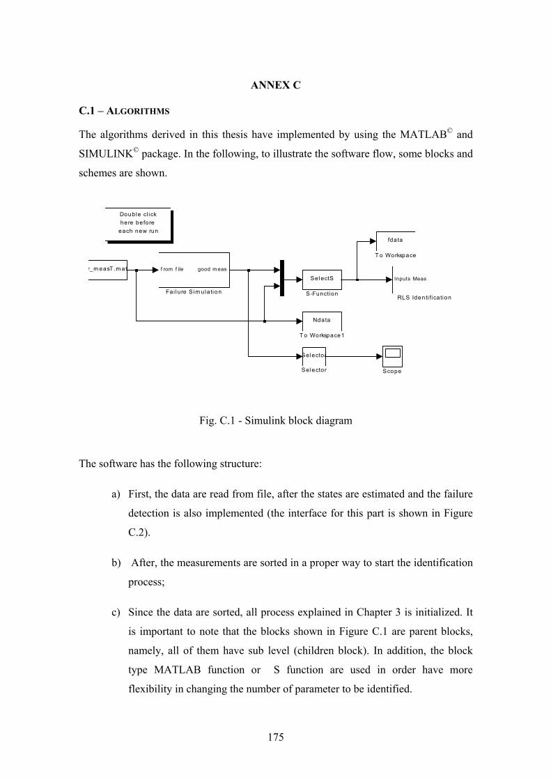
ANNEX C .................................................................................................................... 175 C.1 – Algorithms .......................................................................................................... 175
ANNEX D .................................................................................................................... 179 D.1 – Recursive Least Squares Algorithm – Derivation II.......................................... 179 D.2 – Recursive Least Squares Algorithm with Forgetting Factor .............................. 181
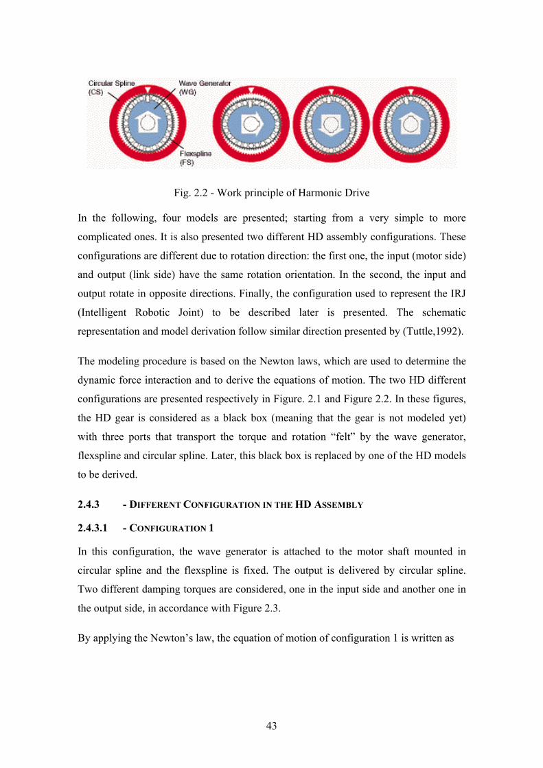
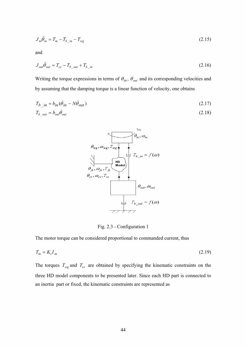
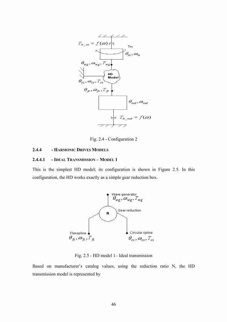
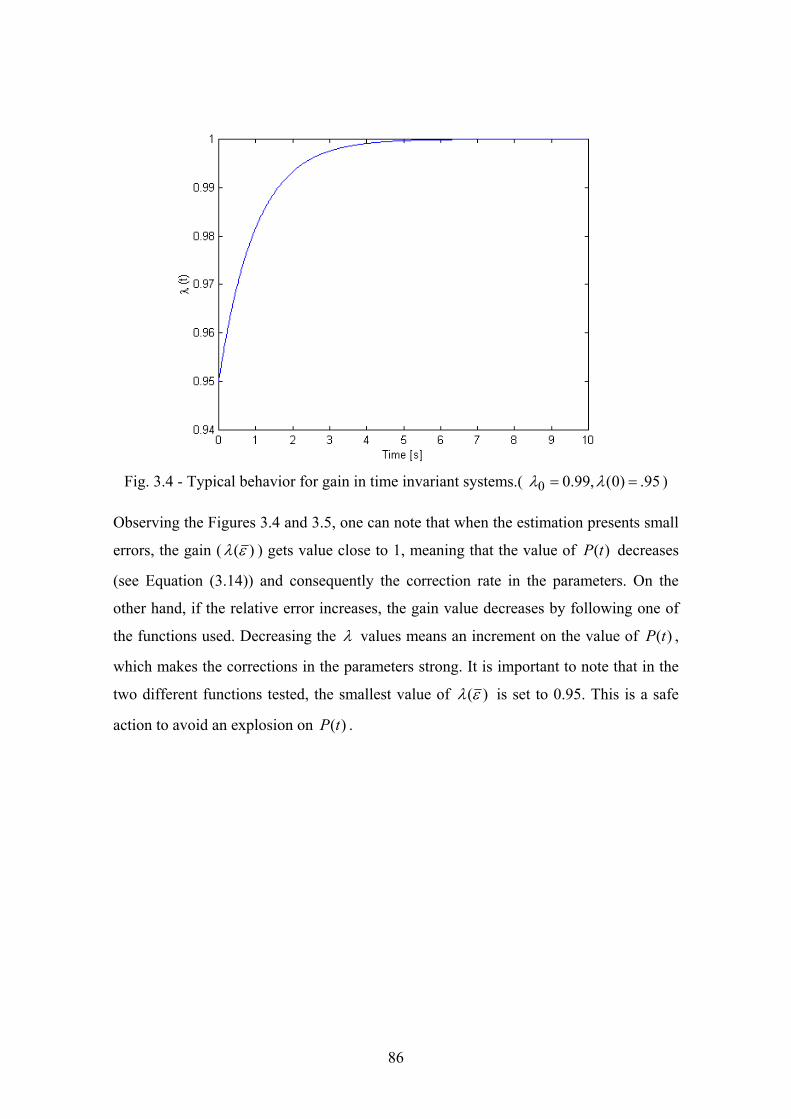
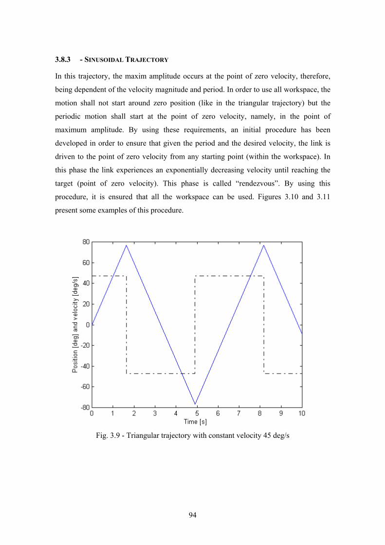
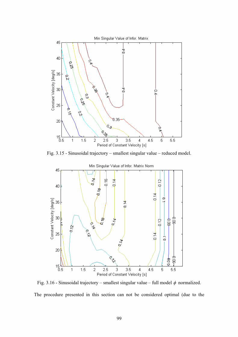
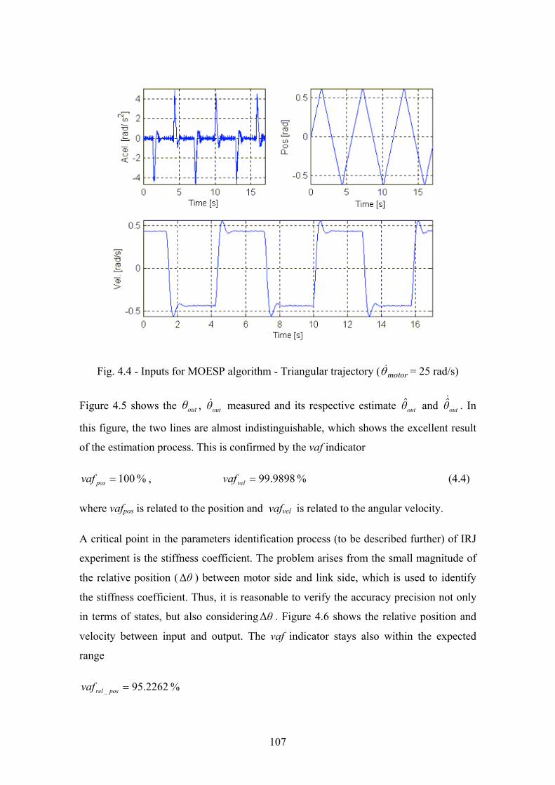
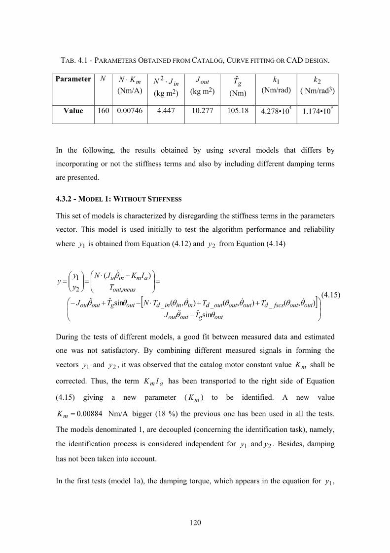
LIST OF FIGURES 2.1 - Internal view of Harmonic Drive .......................................................................... 42 2.2 - Work principle of Harmonic Drive ....................................................................... 43 2.3 - Configuration 1 ..................................................................................................... 44 2.4 - Configuration 2 ..................................................................................................... 46 2.5 - HD model 1– Ideal transmission........................................................................... 46 2.6 - HD model 2 - Incorporating friction losses........................................................... 47 2.7 - HD model 3 – Incorporating friction losses and stiffness..................................... 50 2.8 - HD model 4 – Transmission with friction stiffness, and kinematic error ............. 51 2.9 - Experimental configuration of IRJ for identification............................................ 54 2.10 - Dynamic representation of IRJ experiment......................................................... 55 2.11 - Harmonic Drive model used in IRJ experiment.................................................. 56 2.12 - Stiffness torque for HD type HFUC-25-160-2A-GR.......................................... 58 2.13 - Damping model type 3, Equation (2.77) ............................................................. 61 3.1 - Schematic representation of standard least squares .............................................. 66 3.2 - Schematic representation of MCS algorithm ........................................................ 68 3.3 - General view of the identification scheme............................................................ 80 3.4 - Typical behavior for gain in time invariant systems.( 95.)0(,99.00 == λλ ) ...... 86 3.5 - Behavior of variable gain – Polynomial adjust. .................................................... 87 3.6 - Behavior of variable gain – Exponential function. ............................................... 87 3.7 - Schematic representation of mRLS algorithm ...................................................... 88 3.8 - Schematic representation of the Integrated Algorithm ......................................... 91 3.9 - Triangular trajectory with constant velocity 45 deg/s........................................... 94 3.10 - Sinusoidal trajectory with T (period) = 0.9s, x (0) = 20 deg and v = 15 deg/s ... 95 3.11 - Sinusoidal trajectory with T (period) = 1.9s, x (0) = 20 deg and v = 15 deg/s ... 95 3.12 - Triangular trajectory – smallest singular value – full model. ............................. 96 3.13 - Triangular trajectory – smallest singular value – reduced model ....................... 98 3.14 - Sinusoidal trajectory – smallest singular value- full model. ............................... 98 3.15 - Sinusoidal trajectory – smallest singular value – reduced model. ...................... 99 3.16 - Sinusoidal trajectory – smallest singular value – full model φ normalized. ...... 99 4.1 - Singular values of measurement matrix .............................................................. 104 4.2 - Eigenvalue of matrix A (order 2) ........................................................................ 105 4.3 - Eigenvalue of matrix A (order 3) ....................................................................... 105 4.4 - Inputs for MOESP algorithm - Triangular trajectory ( motorθ& = 25 rad/s) ........... 107 4.5 - Output measurements and respective estimate.................................................... 108 4.6 - Relative position and velocity between input and output side ............................ 109 4.7 - Sensor position failure......................................................................................... 112 4.8 - Link position after measurement reconfiguration ............................................... 112 4.9 - Velocity sensor failure ........................................................................................ 113 4.10 - Link velocity after measurement reconfiguration ............................................. 113 4.11 - Position and velocity sensors failure at different instants ................................. 114 4.12 - Position and velocity after measurements reconfiguration ............................... 115 4.13 - Sensors failure simultaneously.......................................................................... 115 4.14 - Sensor temporary failure ................................................................................... 116 4.15 - Position and velocity after measurement reconfiguration................................. 116 4.16 - Model 1a decoupled – 1y according to Equation (4.15)..................................... 121
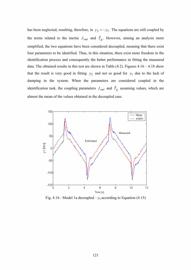
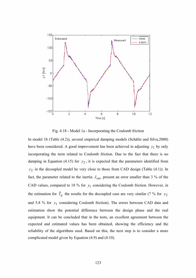
4.18 - Model 1a - Incorporating the Coulomb friction................................................ 123 4.19 - Model 2a - Motor side – Only stiffness term .................................................... 125 4.20 - Model 2a - Link side – Only stiffness term....................................................... 126 4.21 - Model 2b - Motor side – Including damping .................................................... 126 4.22 - Model 2b - Link side – Including damping....................................................... 127 4.23 - Stiffness and damping terms. ............................................................................ 129 4.24 - Damping coefficients ........................................................................................ 130 4.25 - Friction at low velocities ................................................................................... 132 4.26 - Non-linear parameters identification................................................................. 134 4.27 - Linear parameters.............................................................................................. 135 4.28 - Damping parameters ......................................................................................... 135 4.29 - Cyclic phase error ............................................................................................. 136 4.30 - Simulated damping torque ................................................................................ 138 4.31 - Parameters identified by RLS algorithm - Time variant case. .......................... 139 4.32 - Non-linear parameters – Time variant case....................................................... 140 4.33 - Viscous damping identification (link) by using MOESP estimation ................ 142 4.34 - Linear parameters – Using link velocity given by MOESP algorithm. ............ 143 4.35 - Parameters related to damping – Using MOESP estimation............................. 144 4.36 - Linear parameters – Using link position estimated by MOESP algorithm...... 146 4.37 - Damping coefficient– Using link position estimated by MOESP algorithm.... 146 4.38 - Link viscous damping – Using link position estimated by MOESP algorithm 147 4.39 - Linear parameters – Using link position estimated by MOESP algorithm ( 1k
and 2k frozen) .................................................................................................. 147 4.40 - Damping coefficient - Using link position estimated by MOESP algorithm
( 1k and 2k frozen)............................................................................................ 148 4.41 - Link viscous damping – Using link position estimated by MOESP algorithm
( 1k and 2k frozen)............................................................................................ 148 4.42 - Linear Parameters – Simultaneous failure in position and velocity sensor
(state estimated by MOESP) ............................................................................. 149 4.43 - Damping coefficient – Simultaneous failure in position and velocity sensor
(state estimated by MOESP) ............................................................................. 150 4.44 - Link viscous damping – Simultaneous failure in position and velocity sensor
(state estimated by MOESP) ............................................................................. 150 4.45 - Linear Parameters – Simultaneous failure in position and velocity sensor
( 1k and 2k frozen, state estimated by MOESP)............................................... 151 4.46 - Damping coefficient – Simultaneous failure in position and velocity sensor
( 1k and 2k frozen, state estimated by MOESP)............................................... 151 4.47 - Link viscous damping – Simultaneous failure in position and velocity sensor
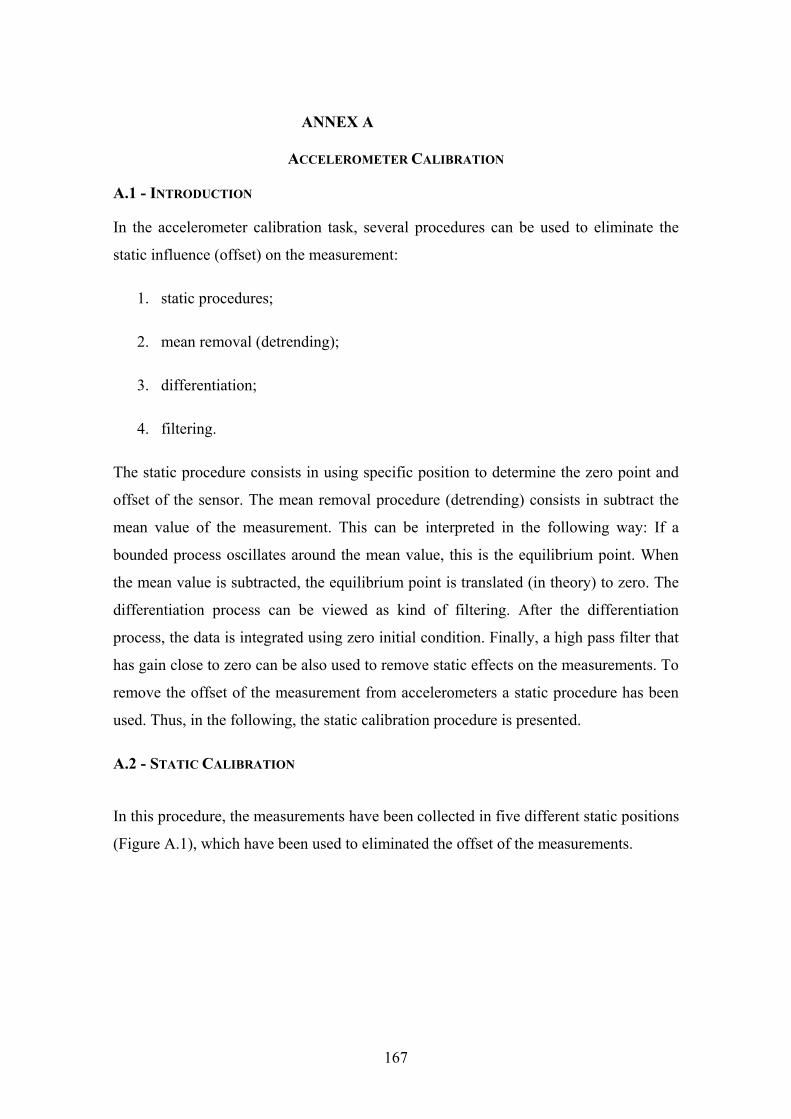
( 1k and 2k frozen, state estimated by MOESP)............................................... 152 . A.1 - Static position for accelerometer calibration..................................................... 168 A.2 - Accelerometer 1 output – Positions: face up and face down ............................. 169 A.3 - Accelerometer 1 output – Positions: horizontal 1 and horizontal 2 ................... 169 A.4 - Accelerometers output – Positions: horizontal 1 for accelerometer 1 and
accelerometer 2 face up..................................................................................... 169 A.5 - Accelerometer 2 output – Positions: face down and horizontal 1...................... 170 B.1 Internal details of IRJ experiment........................................................................ 172 B.3 - Internal view of IRJ experiment ......................................................................... 173
B.4 - Seven joint robot................................................................................................. 174 C.1 - Simulink block diagram ..................................................................................... 175 C.2 - Failure detection interface . ................................................................................ 176 C.3 - Sub level 1 of failure detection and state estimation block. ............................... 177 C.4 - Sub level 2 of the failure detection and state estimation block .......................... 177
LIST OF TABLES
2.1 - Models comparison ............................................................................................... 35 2.2 - Conventional black box models ............................................................................ 38 2.3 - Data of HD type HFUC-20-160-2A-GR............................................................. 57 4.1 - Parameters Obtained from Catalog, Curve fitting or CAD design. .................... 120 4.2 - Parameters Identified for Model 1a (without damping) and 1b (with Coulomb
friction) Equation (4.15). ..................................................................................... 122 4.3 - Identified Parameters for Model 2B – Equation (4.17)....................................... 125 4.4 - Singular Value of Measurement Matrix φ ........................................................ 128 4.5 - Singular Value of Measurement Matrix φ Non-linear Parameters .................. 133 4.6 - Parameters Used in Equation (4.18).................................................................... 137 A2.1 - Sensors Accuracy and Resolution ................................................................... 171
LIST OF SYMBOLS GREEK SYMBOLS ℜ Real Numbers
π Degree of rank variability of MCS Algorithm
ρ Rank of matrix
Η Hankel matrix
Ξ Sub matrix
Σ Diagonal matrix – singular values
δ Precision factor
ω Angular velocity
ε Error
Θ Vector of parameters (to be identified)
φ Matrix of measurements
θ Angular Position
γ Phase of cyclic error
∏ Matrix formed by state space matrices
∆Θ Parameters variation
λ(t) Forgetting factor
η(t) Output of ideal sensors
(.)d Discrete state matrix
σi Singular values
LATIN SYMBOLS [u, v] Interval of search for non-linear optimization
|| . || Euclidian norm
A State matrix (dynamics)
A(q) Polynomial in q
Ai Amplitude of cyclic error (i = 1, 2, ...)
B State matrix (actuators location)
B(q) Polynomial in q
bi Damping coefficients
C State matrix (sensors location)
C(q) Polynomial in q
cs Circular Spline
D State matrix (direct feedback)
D(q) Polynomial in q
e(k) Residual error
f(x) Function to be minimized
fs Flexible Spline
G Hessian matrix
H(.,.) Transfer function
Ia Commanded current
J Index of performance
Jin Input moment of inertia (motor)
Jout Output moment of inertia (link)
k Discrete time index
k1 Linear stiffness coefficient
k2 Cubic stiffness coefficient
Km Motor constant
L(t) RLS gain
N Reduction ratio
R1 Model uncertainty
R2 Sensor uncertainty
s Number of levels in MCS algorithm
T Sampling time
Tg Gravity torque
Ti Torque (i= in, out,...)
u(k) Plant input in instant k
Uk Input vector (Batch estimation)
wg Wave generator (HD)
x(t) state
x* Optimal point
Xk State vector (Batch estimation)
y(k) Plant output at instant k
Z MCS split points
zk Plant output disturbed by noise
LIST OF ACRONYMS AND ABBREVIATIONS
AR Auto Regressive model
ARMAX Auto Regressive model input and Moving Average with exogenous
ARX Auto Regressive model with exogenous input
DLR German Aerospace Center.
HD Harmonic Drive
IRJ Intelligent Robotic Joint experiment
MCS Multi Level Coordinate Search
MIMO Multiple Input and Multiple Output model
MOESP MIMO Output Error State Space Model Identification
RLS Recursive Least Squares
SISO Single Input and Single Output model
SVD Singular Values Decomposition
TS Two – Step Algorithm
25
CHAPTER 1
INTRODUCTION The description of a process in terms of dynamic models is very useful in technological
as well as in scientific fields. Very often, the dynamic models are very important in the
analysis and management of such systems. Given a dynamic system, the goal of the
control system is to keep a pre-determined position even under disturbing effects or
track a reference. In order to design a control system with high performance, it is
essential that the mathematical model, which describes the systems, be accurate. The
proceeding of obtaining a mathematical model based on physical laws and relationships
that describe the behavior of the system is called modeling (Ljung and Söderström,
1983). However, in some special circumstances as in presence of non-linearity, the non-
complete knowledge of the system behavior or because the system has some
unpredictable characteristics, the direct modeling can be inconvenient or not possible. In
these situations, the system information obtained from sensors can be used to build a
mathematical model that describes the system under investigation. This process is called
identification (Ljung and Söderström, 1983). Thus, the main purpose of the
identification process is to obtain a mathematical model, which describes the static as
well as the dynamic characteristics of the system with fidelity. Using this model, tests
and simulations are carried out in order to design a control with high accuracy.
Space missions that use robots and automation have played an important role and
several projects have been developed or proposed in the last decades. Robots when
correctly designed are very effective and present high accuracy in performing their
tasks. Therefore, due to their special characteristics, the robots become very attractive
for applications in space projects. On the other hand, the parameters that describe the
robot dynamics are very sensitive and extremely dependent of environmental condition,
like gravity, temperature, etc. In space missions, the robot is exposed to micro gravity
conditions and also to very big temperature variations. Researches (Heimann, 1999)
have shown that the operating temperature has strong effects on the joint parameters,
damping for instance. These effects can and likely play an important role in the robot
dynamics. In this case, the important characteristics of the robot, which allow high
26
performance, that have been appropriately tested on ground may not fulfill all mission
requirements. The loss of performance occurs because, normally, the control strategy is
based on state feedback and the control parameters that have been optimized (on
ground) no longer will be an optimum. As a result, the whole performance of the robot
is affected. If the mission intends also to verify the behavior of the physical parameters
of a system, an additional task in the identification process shall be carefully selected:
the system structure (model). Thus, there exists a direct relationship between fidelity in
representing the system under investigation and the dynamic model (or model order, if
the state space approach is used). Therefore, when the goal is the identification of
physical parameters, the identification and modeling processes shall be harmonically
integrated.
1.1 - MOTIVATION
The identification of physical parameters is useful in many scientific applications,
especially in the aerospace field and robotics that always require accurate mathematical
models for control purposes; modeling and identification are very important for the
mission success. There exists big diversity of identification methods in time domain as
well as in frequency domain. Some methods use deterministic approaches (Algorithms
based on least squares, for instance), others stochastic approaches (Maximum
likelihood). Besides, these methods are divided into two groups: off-line and on-line.
Due to implementation and convergence problems, the number of on-line algorithms is
limited. In the robotic area, few works focusing on modeling and on-line identification
for physical parameters have been found. On the other hand, on-line algorithms are very
appropriate to be used in high performance control (essentially in adaptive control, for
instance) and also in the physical parameters behavior analysis. A big number of
aerospace systems present some kind of non-linearity, in the robotic systems; this non-
linearity appears due to damping and stiffness effects, which are typical in robots joints.
The problem of non-linearity brings big problem in the identification process, because it
excludes most of the existent identification algorithms. On the other hand, the non-
linear terms are very important when the goal is to study the physical parameters
behavior. The identification process may also not deliver accurate models (or
parameters) if the model used is not appropriate (wrong linearization for instance). This
27
illustrates the strong relationship between identification and modeling.
The robot dynamics is typically complex; this complexity is increased if the robot shall
operate in hostile environments, like in space applications. Under space operational
conditions, the robot dynamics will be affected mainly by big temperature variations,
micro-gravity, material degradation, etc. If the control laws use state information, the
robot performance will be also affected. This problem can be minimized by using an on-
line algorithm, which updates constantly the robot parameters, ensuring optimal
performance in all operational conditions.
Thus, this work represents a further step in the investigations to find new algorithms and
also in the improvement of the existent ones. The derived algorithms can identify both
linear and non-linear parameters. In addition, a detailed modeling of robot joint is
performed and applied to the IRJ experiment. During the research process, it turns out
that the failure situation shall be also considered. Therefore, a strategy and algorithms
that make this problem minimal have been exhaustively investigated and tested. As a
result, an algorithm has been derived that is able to detect and isolate failures in the
essential sensors. The main contributions of this thesis are the detailed modeling of the
robot joint, the investigation, development of news identification algorithms, detection
and failure isolation in sensors. Thus new findings have been observed in modeling,
identification and failure detection fields. All algorithms and strategies developed have
been tested by using real measurements from the IRJ experiment assembled in DLR
(Deutsches Zentrum für Luft - und Raumfahrt).
Finally, it is important to note that all algorithms and strategies derived in this research
for the specific system of a robot can be applied in the identification process of any
dynamic system.
1.2 - REVIEW OF LITERATURE
Many works using the off-line identification approach can be found in the literature.
The techniques presented can be used in the identification process of many dynamic
systems as well as in the robotic field. The majority of these methods are based on the
least squares (LS) approach. The procedures in the identification process are also
similar; the measurements are collected and after processed in order to identify the
28
unknown parameters. In the following, a summary of works related to this thesis is
presented.
1.2.1 - IDENTIFICATION ALGORITHMS
Using a least squares estimator, Fortescue et al (1981) designed an algorithm with a
variable forgetting factor. This algorithm has presented some improvements, avoiding
the explosion of covariance matrix and consequently the control instability. Canudas de
Wit and Carrillo (1990) have presented a modified version of EW-RLS (Exponentially
Weighted RLS) where the forgetting factor has been optimized by using the Lagrange
multipliers technique. The algorithm presented good performance in the applications
where the errors are known (bounded). On the other hand, the algorithm may stop and
do not work properly in some particular conditions. The parametric identification
problem of a system with uncertainty, priori information and bounded noise has been
studied by Tempo (1995) and a worst-case algorithm has been derived. The derived
algorithm belongs to the smoothing class and the main innovation is the computation of
the error by the SVD of the system model. Using the recursive incremental estimation,
the identification problem of a time variant system has been studied by Zhou and Cluet
(1996). In this approach, the system model is assumed to be not a constant but a time
variant one. This approach can be applied in the black box formalism, an ARX model,
for instance. In order to eliminate the bias in the LS estimates, Zhang and Feng (1997)
have proposed a procedure, which uses two filters that are used to filter the system input
and output signals respectively. After, an augmented system with known poles and
zeros is obtained. Using this procedure, the estimation process can be independent of
the noise model used. Based on set membership idea, Bai and Huang (2000) presented a
LMS (Least Mean Square Algorithm) and WRLS estimators focusing the problem of
tracking parameters variations and also decreasing the noise sensibility. In order to
improve track time variant systems, Lozano et al (2000), have introduced modification
in the standard LS algorithm. The modifications have been performed by introducing
additional conditions in the parameters update law as well as in the covariance matrix.
This algorithm gives a bounded estimation and maybe useful in the adaptive control
context, despite of its complexity.
29
1.2.2 - PARAMETERS IDENTIFICATION APPLIED IN ROBOTICS
The identification task applied to robotic systems has received expressive attention in
the last decades. The importance growth comes from the fact that the industries, in order
to fulfill the market requirements have used a lot of automation in the production
process. In the aerospace field, the use of robot becomes common and very attractive,
especially after the ISS (International Space Station) project, because the purposes of
ISS are almost impracticable without use of robots.
The use of identification techniques to improve the reliability in the modeling process
and also to increase the accuracy of the robot task has begun around two decades ago. In
the following, it is presented some works that directly focus the problem studied in this
thesis.
In order to identify the damping and the inertia of a robot equipped with rotary joints,
Olsen and Bekey (1985) have derived a formulation where the dynamic equations are
written in terms of linear combinations of measurements and unknown parameters.
Thus, the parameters can be identified by using a procedure based on a standard least
squares algorithm. Using the Newton-Euler equations to obtain a linear relationship
between measurements and inertial parameters, Atkeson et al (1986) have made some
comparisons between the real model (obtained by identification techniques) and models
obtained from CAD/CAM. The results have shown significant differences between the
models, the accuracy of identified model is expressive. The optimization process has
been carried out by using standard least squares. Using an industrial robot as test bed,
Spechet and Isermann (1988) applied the standard RLS in order to identify some
dynamic parameters like inertia, friction and gravitational force. The strategy used has
shown that the use of an integrated procedure control/identification results in a good
improvement in the robot performance and accuracy. The problem of identifying
parameters in a multi DOF (degree of freedom) robot has been studied by Canudas de
Wit and Aubin (1990). A sequential identification procedure has been proposed. In this
strategy, the identification process starts from the external joints (end effector) to the
internal ones. Therefore, in this process, the parameters that belong to the high level are
considered constant in the lower level. This idea can decrease the number of parameters
to be identified but the coupling effects are lost. The optimization processes can be done
30
by using an off-line (standard least square) or an on-line procedure (WRLS for
instance). In order to design a gain-scheduled control, Gomes and Chrétien (1992) have
written the dynamic equations in an appropriate way (linear combination of parameters
and measurements), making some linearization and using a friction model that is
linearly dependent in the measurement. The results have again shown that the
combination control/identification is very useful, bringing significant improvement in
the accuracy level. Using a simple model (decoupled) and its harmonic solution, Pfeiffer
and Hölzl (1995) have shown that it is possible to recover some dynamic parameters by
applying some static and dynamic torque in the system. This strategy allows that the
identification be simplified. Hanssen et al (2000) has developed a strategy that does not
make use of any force/torque sensor to identify big number manipulator wrist
parameters. In this modeling process, the system is considered as a rigid body and the
final model has been linearized.
In the situation where the goal is just to track the plant output, namely, the physical
meaning of the parameters are out of interest, there exist several ways to perform this
task. If the system has linear behavior or if the non-linearity is not too strong, the
methods ARX, ARMAX, BJ, etc. are able to give satisfactory results. If the system
under investigation has strong non-linearity, the NARMAX (Non-linear ARMAX)
approach should be used. An interesting solution is given by Blaszkowski et al (1998),
the discrete time deconvolution technique has been used to evaluate the system
parameters. Using this technique, the impulse response of a machine tool has been
estimated with good accuracy. By applying the non-linear filtering technique Elhami e
Brookfield (1997) have proposed a sequential identification process of Coulomb friction
and also viscous damping of a robot joint. The big complexity in the modeling process
of a robot joint has been also addressed and an asymmetric model for the Coulomb
friction has been also proposed. It is evidenced the difficulty in modeling (especially,
damping) the robot joint with high fidelity. One can find many works in tribology, the
study of surface contacts, which incorporates three main groups: friction, damage and
lubrication. Armstrong-Helouvry (1991, 1992) presented several empirical models that
try to describe the friction behavior with different levels of fidelity. These works can be
considered as a good starting point in the identification task of friction and damping.
Another relevant work has been performed by Olsson (1992), where several details of
31
damping and friction have been discussed. In addition, a new friction model has been
also proposed.
The effect of temperature variation in the friction behavior has been investigated by
Heimann (1999). It has been shown that the friction in the robot gears is extremely
dependent of operating temperature. The physical parameters have been identified by
using an off-line procedure (standard LS). When high accuracy is required, as in space
applications, it is important to take into account internal characteristics of robot gear.
Due to almost absence of backlash and also thanks to the high reduction ratio obtained
in a very compact mechanism, the Harmonic Drive (HD) has wide application in
robotics as well as in aerospace fields. The HD has a particular construction: it is very
simple from the mechanical point of view but complicated to model if the fidelity level
is high. The main problem in modeling the HD comes from the inherent non-linearity in
the friction part as well as in the stiffness behavior. Marilier and Richard (1989)
presented a simplified model to represent the dynamics of a robot joint. This model has
been used in the control of an industrial robot with success. An exhaustive HD
modeling work has been performed by Tuttle (1992); different HD models are proposed
and a comparative test is also shown. Seyfferth et al (1995) studying the HD dynamics
have proposed a model where the stiffness is represented by a quadratic function. The
hysteresis concept has been also introduced in order to improve the relationship
measurements/models.
The amount of work focusing the analysis and the dynamics of robot with space
purposes is not so big and few works directly related to this subject are found. In the
following, some works related with modeling, models and identification strategy are
presented. Gorter et al (1994) has presented a simplified model for HERA (robot)
reduction joint. The robot HERA originally was idealized to operate in the European
space shuttle HERMES. Several problems related to operations in space and the
inherent effect in the control has been addressed. Using the ETS – VI (Engineering Test
Satellite -VI) as test bed, Adachi et al (2000) have developed an experimental procedure
to check and validate the ETS – VII mathematical model that has been obtained on
ground. The experiment purpose is also to compare two different identification
techniques: a polynomial black box and the subspace approach. Using these two
32
approaches, the main goal is only to estimate the plant (satellite) output given a known
input. There is no interest in either modeling or behavior of physical parameters. In this
comparison, the subspace approach has presented better performance than the
polynomial black box models. The use of subspace methods in robot identification is
not so common due to the typical linear characteristic of these methods. Another
application of subspace identification methods in robotics is presented by Johansson et
al (2000). Several subspace-based methods have been tested and compared. In parallel,
a procedure to evaluate the friction force in the robot joint has been also proposed. Shi
et al (2000) developed an experiment to investigate the robot dynamics in operational
conditions similar to that ones encountered in space. The experiment consists in a two-
joint articulated manipulator horizontally assembled under effect of airflow. The friction
in the joint has been identified independently; only the HD has been used, in the test the
link has been removed. It has been shown that the identification is extremely useful in
the process of gathering precise mathematical models.
In the robot identification process, it is necessary to follow some standard steps; one of
them is the selection of the trajectory that will ensure that all parameters are properly
excited. There exist several procedures that allow one to obtain an optimal trajectory.
Swevers et al (1997) have proposed an interesting procedure that makes use of a series
of sine and cosine to design an optimal trajectory. This strategy is efficient if the gears
are considered as a rigid body, but can not be directly applied if a new degree of
freedom (stiffness) is introduced in the gear model. Another theory that is commonly
used to check the excitation levels is the minimization of the measurement matrix
condition number. This approach has been applied by Armstrong (1987) and Heimann
(1999).
1.2.3 - SENSORS FAILURE
The problem of detecting and isolating failures is extremely important in engineering
systems. In the literature, two approaches can be found: one that is based on hardware
redundancy and another one that uses filtering and analytical theory. Although this field
is very wide and offers different options to detect and isolate failures, this thesis
contributes with a simple and efficient algorithm based on state space identification. In
the following, some related works are focused.
33
The detection and failure isolation in linear systems has been studied by Caglayan
(1980). An algorithm based on LMS (Least mean squares) has been derived, where its
main characteristic is the reduced number of filters used in the detection and isolation
process. A good survey focusing different approaches and useful techniques in detection
and failure isolation is presented by Gertler (1988). Using the analytical redundancy
strategy, Yang et al (1988) have presented a procedure based on master and slave ideas
to detect failures in systems where the parameters are not completely known. The
implementation of this idea has been carried out by using a RLS estimator. In practice,
such procedure restarts the estimator when the errors are bigger than a specified value.
This strategy can be successfully applied in problems where the main goal is to estimate
the plant output, only. Using the state-space identification approach, Zimmerman and
Lyder (1993), presented a strategy to diagnose failures in sensors mounted in flexible
structures. The detection process is based on the analysis of the state-space matrices
rather than in the output of a bank of filters that are commonly used. This approach
associated to state-space identification becomes very interesting because it allows one to
detect and also to determine the possible failure characteristics. Applying the bilinear
theory, Yu and Shields (1996) proposed a bilinear filter that uses unknown inputs. Such
algorithm has been applied in a hydraulic machine and the results are satisfactory if
some restrictions in the error matrix are satisfied. Another survey focusing the problem
of failure detection and isolation has been presented by Leohardt and Ayoubi (1997). In
this survey, the use of Artificial Intelligence like neural network, fuzzy logic and
genetic algorithm in the failure detection problem has been also discussed. An extensive
study in the failure detection and isolation procedures is presented by Basseville (1997).
Several criteria to monitor the residues and to choose the decision rules are presented.
Using the minimax approach, Yin (1998) present a procedure to classify and detect
failures. The procedure is designed in such a way that a balance between robustness and
optimality is obtained. The minimax procedure is used to minimize the maximum
number of false failure that is previously declared. The problem of detecting and
isolating multiply failures has been studied by Keller (1999). A special form of Kalman
filter is used to detect and isolate failure that can occur sequentially or simultaneously.
When a failure is declared, the correspondent component is removed from the
estimation process, minimizing the effect in the states are to be estimated.
34
35
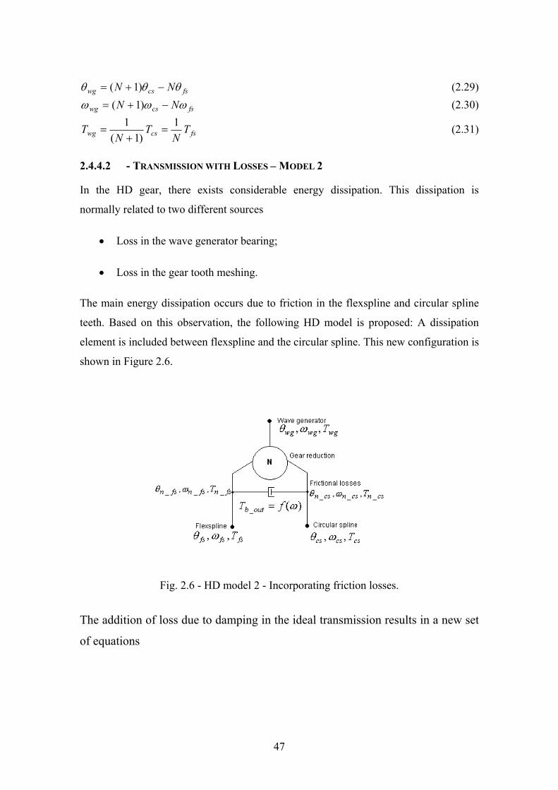
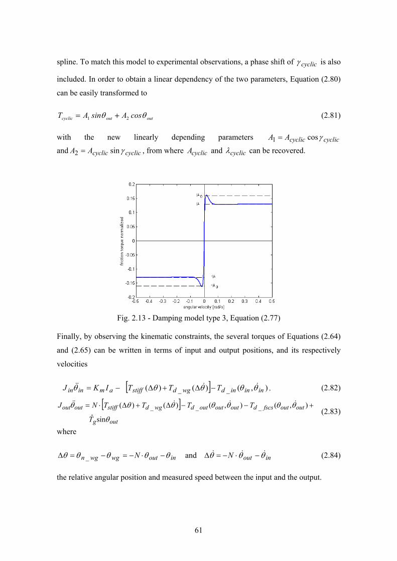
CHAPTER 2
MODELS AND MODELING 2.1 - INTRODUCTION
Normally, the parameters identification is based on models or structures that are
responsible for the representation of the physical system under investigation.
There exist several ways to represent a real system. This representation can be
performed by using differential equations that govern the system, recurrence
equations, state-space models, etc. The last two alternatives are commonly
known as black-box formalism. This idea comes from the fact that the main goal
is only to estimate the plant output given the inputs and the previous outputs. The
parameters meaning or the “dynamic” that govern the system is out of interest. In
such models, the estimation accuracy is obtained by adjusting the number of
previous past outputs to be used or by selecting the system order, in case of state-
space representation. The choice between models represented by differential
equations or by black box models depends exclusively on the requirements to be
fulfilled. The models where the parameters have physical meaning are called
phenomenological models, the models where the parameters do not have physical
meaning are called behavioral models. Table 2.1 shows the main characteristics
of these two classes of models.
Phenomenological models Behavioral models Parameters Have a concrete meaning Do not have concrete meaning
Simulation effort &
Processing time Hard and slow Easy and quick
Priori information Taken into account Not taken into account Validity Domain Wide (if the structure is
correct) Restricted
Although, the main purpose of this thesis is the identification of physical parameters,
namely phenomenological models, in the following some classical black box models are
TAB. 2.1 - MODELS COMPARISON
36
presented. This kind of identification approach (black box) is used in the failure
detection strategy to be presented later.
2.2 - BLACK BOX MODELS
2.2.1 - ARX MODEL
The ARX model is directly related with a transfer function of the system. This is one of
the simplest models of transfer function and this is the reason because it is widely used.
The ARX model is defined as a linear difference equation between inputs and outputs.
For a SISO system, the ARX model is written as
)()()()()()( 11 kenkubikubnkyaikyaky bbnaan +−++−=−++−+ LL (2.1) where k = time index
)( iky − = output in previous instant )( iku − = input in previous instant
)(ke = residual error an = number of a coefficients bn = number of b coefficients
Equation (2.1) can be written as
)()()()()( kekuqBkyqA += (2.2) where the polynomials )(qA and )(qB are defined in terms of the delay operator 1−q
anan qaqaqA −− +++= L1
11)(
bnbn qbqbqB −− ++= L1
1)(
The term )()( kyqA in Equation (2.2) corresponds to the AR parcel (Auto Regressive) of
ARX model and the term )()( kuqB corresponds to the external input. Equation (2.2) can
be re- written in transfer function form
37
)()(
1)()()()( ke
qAku
qAqBky += (2.3)
The term )()(
qAqB represents the plant discrete transfer function.
2.2.2 - ARMAX MODEL
The ARMAX model is similar to ARX model, which uses a sequence of past inputs that
are filtered by the model. However, the ARMAX model also filters the residual errors
aiming at a better disturbance characterization. In analogy with the ARX model, the
ARMAX model can be considered as transfer function of the system that is being
identified.
For SISO systems, the difference equations ARMAX is written as
)(
)()()()()()()( 111
ccn
bbnaan
nkec
ikeckenkubikubnkyaikyaky
−+
+−++−++−=−++−+ LLL
(2.4) where
)( ike − = is a white noise in the previous inputs
cn = is the number of c coefficients Similarly to ARX model, the ARMAX model is written as
)()()()()()( keqCkuqBkyqA += (2.5) where )(qA and )(qB are the same as already defined in ARX model and )(qC is
defined as
cncn qcqcqC −− ++= L1
1)(
The ARMAX model incorporates the additional term )()( keqC that is correspondent to
moving average part.
Writing Equation (2.5) in transfer function form one obtains
38
)()()()(
)()()( ke
qAqCku
qAqBky += (2.6)
Similarly to ARX model, the term )()(
qAqB is the discrete transfer function of the system
and )()(
qAqC works like a filter in the residual error.
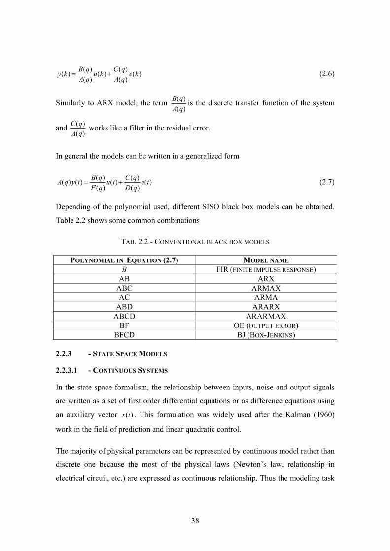
In general the models can be written in a generalized form
)()()()(
)()()()( te
qDqCtu
qFqBtyqA += (2.7)
Depending of the polynomial used, different SISO black box models can be obtained.
Table 2.2 shows some common combinations
TAB. 2.2 - CONVENTIONAL BLACK BOX MODELS
2.2.3 - STATE SPACE MODELS
2.2.3.1 - CONTINUOUS SYSTEMS
In the state space formalism, the relationship between inputs, noise and output signals
are written as a set of first order differential equations or as difference equations using
an auxiliary vector )(tx . This formulation was widely used after the Kalman (1960)
work in the field of prediction and linear quadratic control.
The majority of physical parameters can be represented by continuous model rather than
discrete one because the most of the physical laws (Newton’s law, relationship in
electrical circuit, etc.) are expressed as continuous relationship. Thus the modeling task
POLYNOMIAL IN EQUATION (2.7) MODEL NAME B FIR (FINITE IMPULSE RESPONSE)
AB ARX ABC ARMAX AC ARMA
ABD ARARX ABCD ARARMAX
BF OE (OUTPUT ERROR) BFCD BJ (BOX-JENKINS)
39
normally leads to representation in the form
)()()()()( tuBtxAtx Θ+Θ=& (2.8) where the matrices BA and have appropriate dimensions ( nn × and mn × , respectively
for an n dimensional state and an m dimensional control vector). The differentiation
with respect to that time is represented by a dot over the variable, besides the vector Θ
typically corresponds to unknown physical parameters, material constants, etc.
Modeling, normally is performed in terms of state variables that have physical meaning
(position, velocity, etc.) and the output is normally a combination of the states. Defining
)(tη as the output of ideal sensors
)()( tCxt =η (2.9) defining p as differentiation operator, Equation (2.8) is written as
[ ] )()()()( tuBtxApI θθ =− (2.10) meaning that the transfer function between η and u in Equation (2.9) is
[ ] )()(),(
)(),()(1 θθθ
θη
BApICpH
tupHt−−=
= (2.11)
Thus, it is obtained a system transfer function model, which is parameterized in terms of
physical coefficients.
2.2.3.2 - DISCRETE SYSTEMS
Since most of the studies make use of computational process and also due to data
acquisition process, normally it is necessary to represent the systems in discrete form.
By assuming that the inputs are constant during one sampling time T
TktkTkTuutu k )1( ),()( +≤≤== (2.12) then Equation (2.8) is easily solved from kTt = to TkTt +=
)()()()()( kTuBkTxATkTx dd θθ +=+ (2.13)
40
where TAd eA )(θ=
τθτ
τθ dBeBT
Ad ∫
==
0
)( )(
Similarly to Equation (2.11), the system discrete transfer function model is represented
C N= . The exponential coefficient Sδ is assumed to be 1.
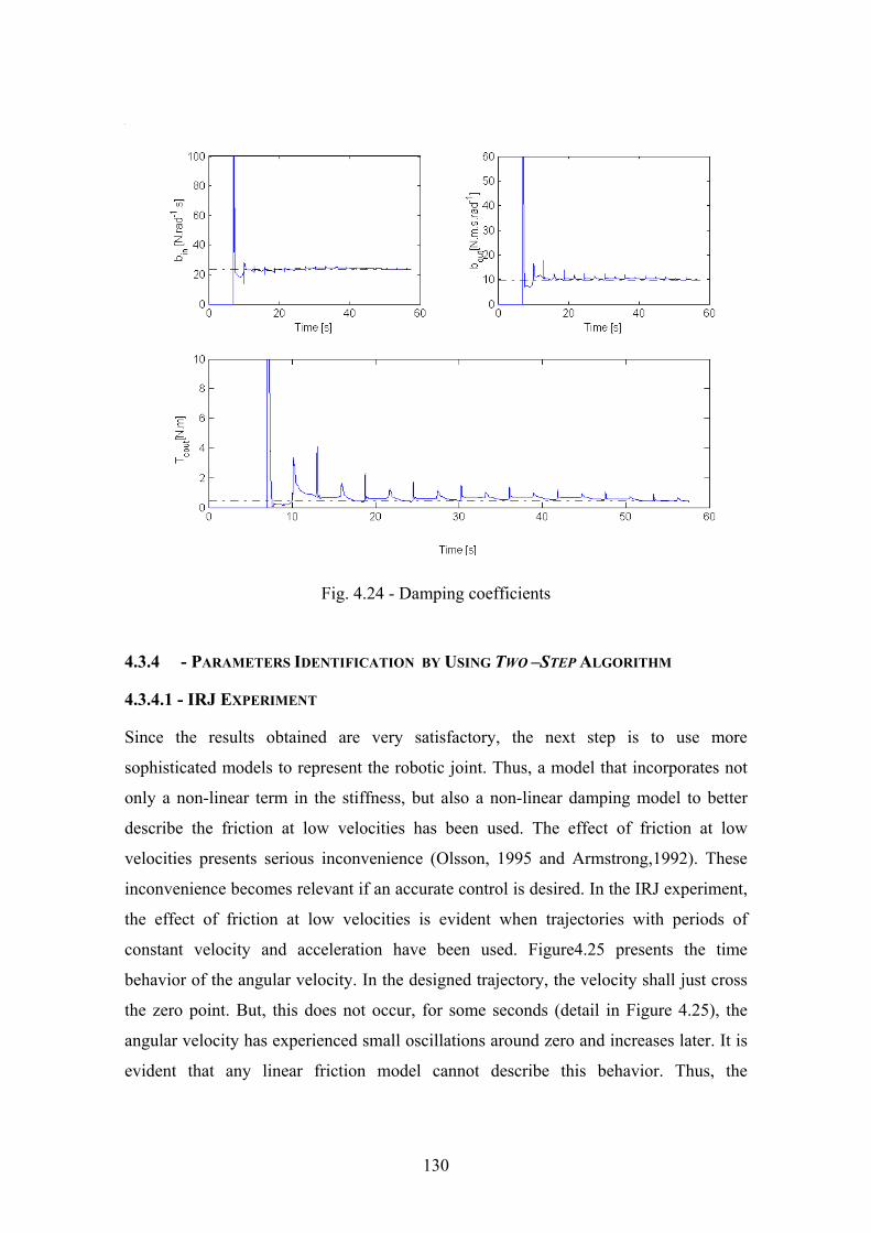
132
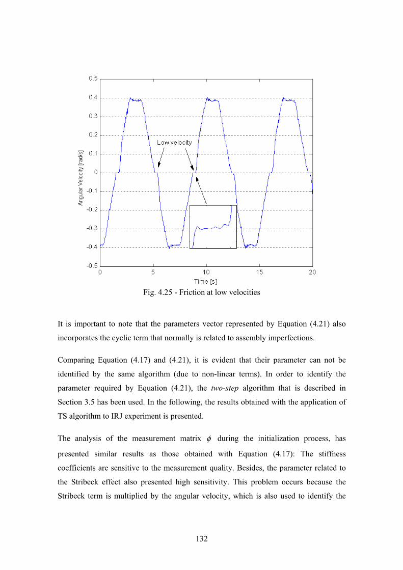
Fig. 4.25 - Friction at low velocities
It is important to note that the parameters vector represented by Equation (4.21) also
incorporates the cyclic term that normally is related to assembly imperfections.
Comparing Equation (4.17) and (4.21), it is evident that their parameter can not be
identified by the same algorithm (due to non-linear terms). In order to identify the
parameter required by Equation (4.21), the two-step algorithm that is described in
Section 3.5 has been used. In the following, the results obtained with the application of
TS algorithm to IRJ experiment is presented.
The analysis of the measurement matrix φ during the initialization process, has
presented similar results as those obtained with Equation (4.17): The stiffness
coefficients are sensitive to the measurement quality. Besides, the parameter related to
the Stribeck effect also presented high sensitivity. This problem occurs because the
Stribeck term is multiplied by the angular velocity, which is also used to identify the
133
viscous damping. The matrix rank is preserved, but the sensitivity is affected. The
singular value of measurement matrix is shown in Table (4.5).
Parameter 1k 2k ak 1C 2C inb outb
Sing. Val. 0.0338 1.33e-7 18.0883 35.8555 0.0272 15.5951 15.6339
Parameter 1A 2A
Sing. Val. 12.3118 33.8440
Figure 4.26 shows the optimization process by using the MCS algorithm. It can be
noted that after a few iterations, the MCS algorithm fulfills all the convergence
requirements. After the identification of non-linear parameters, the on-line identification
of the linear parameters is initialized. In this period, the non-linear parameters kept
constant and the MCS algorithm is waiting for operating if the norm error increases.
Using this strategy, one can obtain an on-line update in the linear parameters and a
random correction (only when the error norm increases) in the non-linear parameters.
This procedure offers a remarkable gain in the computer effort, allowing the inclusion
of non-linear terms in the parameters vector for on-line identification.
In the figures to be presented, the constant dashed line represents the parameters value
obtained by applying off-line methods using all measurements available. Figure4.27
shows the identification results related to the stiffness terms and also related to 1C . It
can be noted that the linear stiffness term has fast convergence to the off-line value
despite of its high sensibility. The cubic stiffness term is more sensitive and presented
more oscillations. However, the algorithm presented enough robustness to overcome
these critical points and converges to the expected value. The parameter correspondent
to the additional spring and to 1C , in agreement with the singular values analysis, are
very stable and presented fast convergence.
TAB. 4.5 - SINGULAR VALUE OF MEASUREMENT MATRIX φ NON-LINEAR PARAMETERS
134
Fig. 4.26 - Non-linear parameters identification Figure 4.28 shows the behavior of 2C , viscous damping (in both sides) and also the
amplitude of cyclic error (normally related to assembly imperfections). In agreement
with the preliminary analysis, the 2C behavior has presented sensitivity bigger than
other parameters. However, the recursive identification after some seconds converges to
the value obtained in the off-line procedure. The viscous damping in the motor side also
presented oscillations and after a short transient converges to the expected values. The
parameter related to the cyclic error presented also stable behavior and its magnitude is
around 3.7 Nm. The phase γ can be considered zero (0.050). The phase behavior is
shown in Figure 4.29. It is important to note that the identification of cyclic phase error
may not be an easy task. This parameter is related to values obtained from trigonometric
functions, which may present small variations depending of robot workspace. However,
It can be noted that the recursive identification always asymptotically converges to the
reference values.
135
Fig. 4.27 - Linear parameters
Fig. 4.28 - Damping parameters
136
Fig. 4.29 - Cyclic phase error
The results have shown the robustness and efficiency of the TS algorithm in
identifying the stiffness and damping parameters of IRJ the experiment. It can be
noted that even in the case where not all parameters have good sensitivity, the
algorithm always deliver coherent results that agree with the values obtained
from other methods. It is also important to stress that in the presented results all
measurements have been obtained from sensors placed in the IRJ experiment. No
simulated data have been used.
4.3.4.2 - TIME VARIANT SYSTEMS
Many times, the system under investigation presents variations, mainly due to
environmental changes. Thus, it is interesting to test the ability of the TS algorithm in
tracking the non-linear parameters, since the linear parameters are continuously updated
by the RLS algorithm. In order to perform these tests, hybrid (measured and simulated)
data is used. The simulated data is used to represent variations in the non-linear
137
parameters. The angular velocity has been taken from the experiment and the stiffness
torque has been calculated by defining values for the parameters that appear in Equation
(4.18). The parameter Sδ is set to 1 and the other ones are given in Table (4.6)
Parameter Value
inb 9 Nm.s.rad-1
µTN ⋅|| 29 Nm 1
2|| −⋅ωTN 480Nm
1ω 0.0595 rad.s-1
Sω 0.0251 rad.s-1
By using the values from Table (4.6) and the measured velocity, the friction
torque( indT _ ) has been simulated. The torque behavior is shown in Figure 4.30.
Using indT _ as a reference for the TS algorithm, a system that experiences variations in
the non-linear parameters has been simulated. At time t = 16 s, the reference torque has
been recalculated and the linear parameters have been increased by 30 % of their
nominal values (Table4.6). The non-linear parameters have been modified at time t = 27
s, when their values has been increased by 20 %. The changes in the nominal values try
to simulate system operational changes.
TAB. 4.6 - PARAMETERS USED IN EQUATION (4.18)
138
Fig. 4.30 - Simulated damping torque
Figure 4.31 shows the linear parameters behavior during identification process. It can be
noted that during the starting procedure when both (linear and non-linear) parameters
are being optimized, the linear parameters presented a typical transient oscillation,
converging after to the nominal values. When the linear parameters are changed (t = 16
s), the RLS algorithm efficiently updates the parameters and converges to the new
nominal values. This is represented by the small jumps in Figure 4.31. The changes in
the linear parameters do not affect the non-linear ones (Figure 4.32). This is possible
because the RLS has fast response, keeping the errors below the value required to
activate the MCS algorithm. On the other hand, the change in the non-linear parameters
affects the linear ones. This occurs because the errors are bigger than the required value
to activate the MCS. The MCS algorithm does not have fast response like RLS. In fact,
in this period, the algorithm behaves in similar manner than in the starting procedure;
the only difference is because the linear parameters are now almost optimized.
139
Fig. 4.31 - Parameters identified by RLS algorithm - Time variant case.
It can be noted that the TS algorithm offers the possibility to identify non-linear
parameters (recursively) at extremely low computational cost. The non-linear algorithm
is activated only in the starting procedure or in case of an expressive change in the
operational conditions. This allows one to obtain a real-time procedure even in cases
where non-linear terms are included in the identification process. The recursive
identification is not possible only in short time interval, when the non-linear
optimization algorithm is activated. Another point to be stressed is related to the initial
conditions. Non-linear optimization algorithms are extremely depending on the initial
conditions, the number of variables to be optimized and even on the profile of the
objective function. As a result, the local optimizer many times found false solutions and
global methods (like MCS) may become excessively slow and sometimes, solution
degradation occurs. Thus, one can conclude that the TS algorithm fulfills most of the
inherent problems of non-linear systems identification, such as
• Computer load;
• Possibility of recursive identification;
140
• Reduction of the parameters to be identified by the non-linear algorithms;
Fig. 4.32 - Non-linear parameters – Time variant case
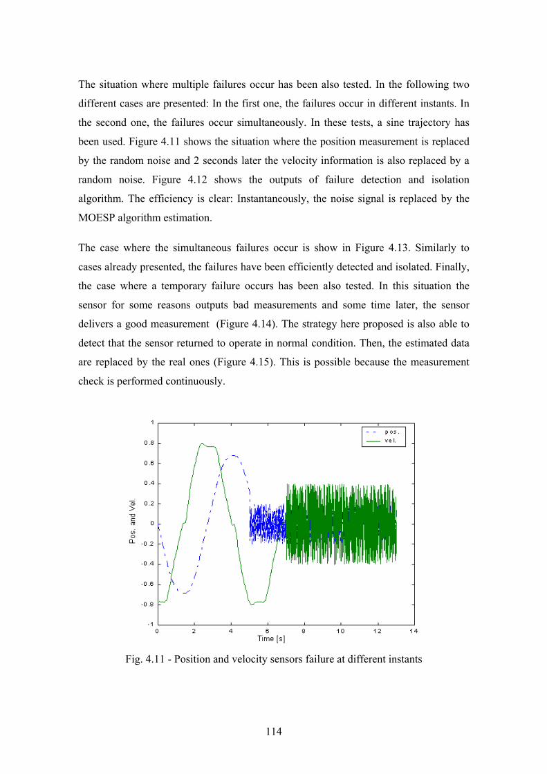
4.4 - IDENTIFICATION UNDER FAILURE CONDITIONS
The identification techniques require not only a minimal number of measurements but
also that these measurements are of good quality. In specific cases the IRJ experiment,
may operate also in space environment. This fact shows that a special attention to the
sensors and actuators shall be dispensed. Thus, during this research strategies and
alternatives have been developed in order to investigate the special requirement for this
task. An important detail to be considered is related to failure in sensors. Thus, aiming
to maximize the available experiment information in case of failure occurrence, two
solutions are presented:
• Algorithm reconfiguration;
• Stiffness isolation.
141
It is important to note that the solutions proposed always try to maintain the low
computer effort and also to keep the algorithm reconfiguration ability. The first
requirement is needed because there exists the possibility to have on-board processing ,
normally the on-board computer has limited characteristics if compared to computers
used on ground. The second requirement is needed because there is a high possibility of
the system present time variant behavior. Therefore, the main requirements for the
algorithm and strategy to be developed are: adaptation capability, reconfiguration and
low computer effort.
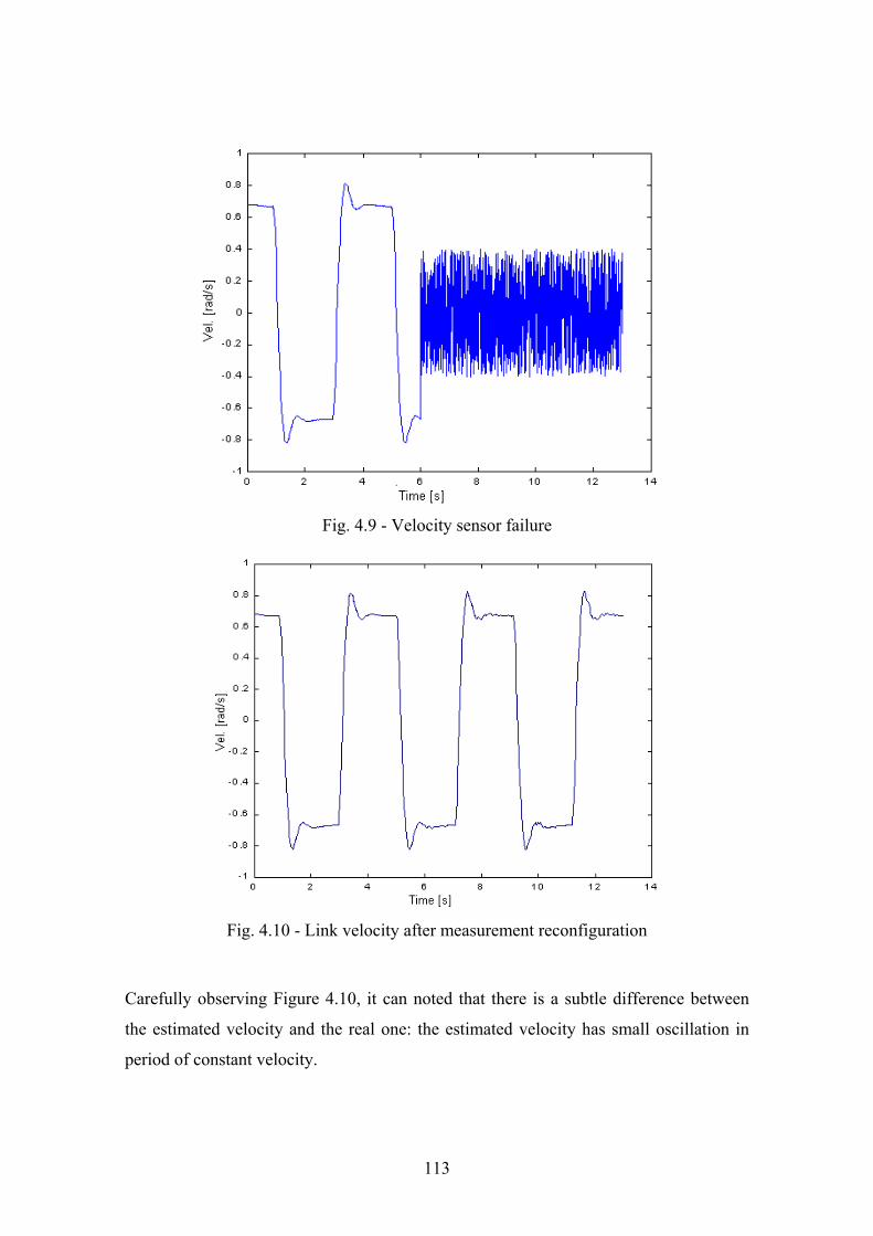
4.4.1 - FAILURE IN VELOCITY SENSOR
In the following, the parameters obtained by using TS algorithm under link velocity
sensor failure (simulated) are presented. In the detection, isolation and estimation
process, the procedure described in Section 4.2 has been used. The model used is
described by Equation (4.21), namely, the model incorporates the non-linear terms and
cyclic errors.
The failure in the link velocity sensor is programmed to occur at t = 20s, and the
corresponding measurement signal has been replaced by random noise (0,0.1). From
this moment, the information given by this sensor is replaced by the MOESP estimation.
The behavior of the identification by using MOESP estimation is shown in Figure 4.33.
It is observed that the accuracy given by the vaf indicator is confirmed. No oscillations
have been observed after replacing the measured data by the estimated ones. The dashed
line in Figure 4.33 represents the values obtained by he off-line identification using only
measured data. It can be noted that the TS algorithm converges to the expected value
using estimated state. This ensures that mission success is guaranteed even in the case
of link velocity sensor failure.
142
Fig. 4.33 - Viscous damping identification (link) by using MOESP estimation
In Figure 4.34 the stiffness and damping parameters are also shown. It can be noted that
all parameters have similar behavior as those presented in Figure 4.27 and 4.28. This
means that the estimation given by MOESP algorithm has no big effect in the global
identification process.
4.4.2 - POSITION SENSOR FAILURE
The coefficient related to the system stiffness is extremely sensitive (this is already
shown by the correspondent singular value) to the measurement quality. This fact is
directly related to the magnitude of measurements to be used. The linear stiffness
coefficient for instance, is related to measurements with magnitude 10-3; the cubic
coefficient is related to measurement of magnitude of 10-9. Although, the MOESP
algorithm gives an excellent state estimation, it is almost impossible to maintain the
estimated data equal or better than the measured one. In the face to this problem, two
solutions have been found that are aiming to minimize the state estimation effect in the
stiffness and 2C . These alternatives are presented in the following..
143
Fig. 4.34 - Linear parameters – Using link velocity given by MOESP algorithm.
4.4.2.1 - ALTERNATIVE 1 – RECONFIGURATION OF IDENTIFICATION ALGORITHM
The first alternative is just to keep the algorithm that identifies the parameters using the
MOESP estimation. The only change is in the term 2R (confidence in the sensors
output) of the RLS algorithm. In this case, as expected, after failure detection and
isolation process, the parameters slide from the nominal values and converge to a new
value, which is assumed as “nominal”.
144
Fig. 4.35 - Parameters related to damping – Using MOESP estimation The link position sensor failure has been scheduled to occur at t = 20s. After the alarm,
immediately all identification process is reconfigured where the following actions have
been made:
• Replace the output of sensor under sensor failure by the correspondent MOESP
estimation;
• Automatic change in the value of 2R of RLS algorithm.
In Figure 4.36 – 4.38 the identification results are shown in the case where the MOESP
estimation has been used. Considering the severe requirements (measurements of
magnitude 10-9) for stiffness parameters, one can conclude that the results are excellent.
The parameters present small changes in comparison with the values obtained by off-
line estimation using only measured data. The variations in the parameters range from
0.5 % (additional spring) to 10.5 % (term related to the Stribeck effect). The variation in
2C is justified by the high sensitivity of this term indicated in the singular value
145
analysis. Once, the identification process is reconfigured, and considering that the
estimation is very good, there exist still a difference between measured and estimated
ones. This difference is naturally reflected more sensitively in the parameters.
4.4.2.2 - ALTERNATIVE 2 – RECONFIGURATION OF ALGORITHM AND FREEZING OF STIFFNESS COEFFICIENT
Besides the actions taken in Section 4.4.2.1, in this situation, the parameters related to
the stiffness term have been frozen in their last value acquired before the failure alarm
happens. In this case, the reconfiguration action also eliminates the parameters 1k and
2k from the vector Θ .
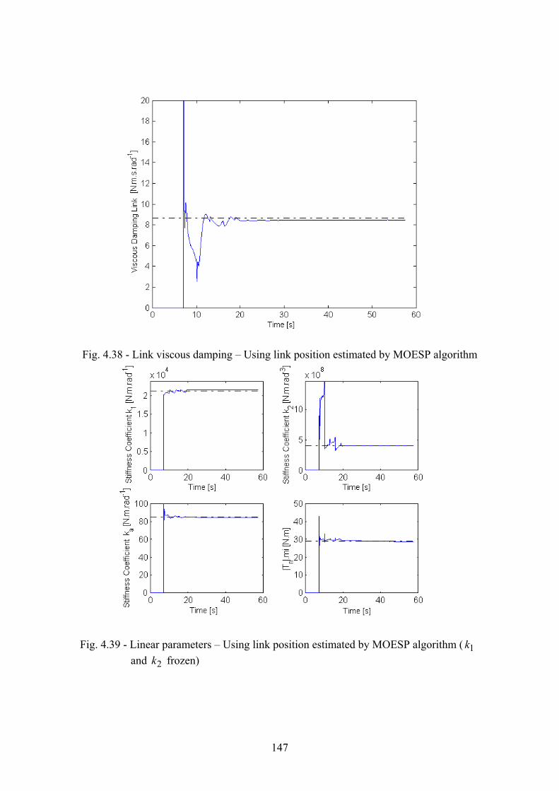
The results obtained by using this strategy are presented in Figures 4.39 – 4.41. A
similar behavior of the strategy presented in Section 4.4.2.1 can be noted: all parameters
present variations from 0.5 % to 10.5%. The difference is because here, the parameters
1k and 2k are kept constant. The impact on the identification process can be described
in the following manner: By one side, when the two elements are removed from the
parameters vector, the system degree of freedom has decreased. This decreases the
model ability in tracking the reference value. On the other hand, when the number of
parameters to be identified is reduced, the algorithm performance increases. Therefore,
in the case studied, these two situations, , almost annihilate the effect one of the other.
This justifies the similarity with the strategy presented in Section 4.4.2.1.
146
Fig. 4.36 - Linear parameters – Using link position estimated by MOESP algorithm
Fig. 4.37 - Damping coefficient– Using link position estimated by MOESP algorithm
147
Fig. 4.38 - Link viscous damping – Using link position estimated by MOESP algorithm
Fig. 4.39 - Linear parameters – Using link position estimated by MOESP algorithm ( 1k
and 2k frozen)
148
Fig. 4.40 - Damping coefficient - Using link position estimated by MOESP algorithm
( 1k and 2k frozen)
Fig. 4.41 - Link viscous damping – Using link position estimated by MOESP algorithm
( 1k and 2k frozen)
149
4.4.3 - SIMULTANEOUS FAILURE IN POSITION AND VELOCITY SENSORS.
The case where both sensors, position and angular velocity, present failure have been
also studied. In accordance with the analysis already presented for isolated sensor
failure, the results are very similar to the case where the position sensor is failed. This is
expected, since the failure in velocity sensor has no big impact on the identification
process. Using the same strategy shown in the case of isolated failure, two alternatives
have been tested: one where the stiffness coefficients are identified after algorithm
reconfiguration and another where the stiffness coefficients are frozen in their last value
acquired before the failure alarm happens. The failure have been adjusted to occur at
time t = 20 s. After this instant, the measurements of link position and velocity are
replaced by random noise (0,0.1), all identification process is reconfigured and the
position and velocity information is given by the MOESP algorithm. Figures 4.42 –
4.44 show the results obtained after the algorithm reconfiguration. The stiffness terms
are also identified. The case where the stiffness parameters are frozen is shown in
Figure 4.45 – 4.47.
Fig. 4.42 - Linear Parameters – Simultaneous failure in position and velocity sensor
(state estimated by MOESP)
150
Fig. 4.43 - Damping coefficient – Simultaneous failure in position and velocity sensor
(state estimated by MOESP)
Fig. 4.44 - Link viscous damping – Simultaneous failure in position and velocity sensor
(state estimated by MOESP)
151
Fig. 4.45 - Linear Parameters – Simultaneous failure in position and velocity sensor ( 1k
and 2k frozen, state estimated by MOESP)
Fig. 4.46 - Damping coefficient – Simultaneous failure in position and velocity sensor
( 1k and 2k frozen, state estimated by MOESP)
152
Fig. 4.47 - Link viscous damping – Simultaneous failure in position and velocity sensor
( 1k and 2k frozen, state estimated by MOESP) 4.5 - SUMMARY
In this Chapter, the applications of the strategies and algorithms derived in the previous
Chapters are presented. A big number of dynamic models has been used and tested. The
complexity of such models has been continuously increased and the effect of each term
has been analyzed. A failure detection and isolation procedure, which requires low
computer effort has been also presented.
All proposed algorithms and strategies developed presented excellent results concerning
accuracy as well as computer effort. The TS algorithm shows efficiency in the
identification process using measured data (IRJ experiment) as well as in case where
time variant systems have been simulated.
The integrated process (identification and failure isolation) show efficiency in the
failure detection and isolation of the data under failure suspect. Due to critical
conditions of the identification of stiffness coefficients, one can conclude that the results
obtained in identification process by using MOESP estimates are remarkable. Based on
these results, applications for those strategies can be immediately suggested, in the
adaptive control are design for instance.
153
CHAPTER 5
CONCLUSION AND RECOMMENDATIONS
5.1 - CONCLUSIONS
The modeling process is extremely important in the system analysis as well as in the
control. Normally, the complexity of the model increases proportionally to the level of
the desired fidelity in system modeling. The more complex the model is, in theory, the
closer we are to the real system. On the other hand, complex models normally present
non-linear terms, which add severe restrictions to the identification process.
In this thesis, a detailed mathematical modeling of a robot joint is presented, where not
only non-linear terms related to the stiffness have been incorporated but also related to
different damping models. The modeling process is started by assuming very simple
models. The model complexity level has been analyzed aiming at a good balance
between accuracy and the impact that the addition of the new term brings to the
identification process. All derived models have been used in analyzing and studying of
the IRJ experiment, where excellent results have been obtained.
When the mathematical model has been assumed satisfactory, the next step was to
choose the trajectory type that improves the excitation of the physical parameters to be
identified. If the robot joint is considered a rigid one, the task to obtain an optimal
trajectory is not complicated, since there are procedures that analytically deliver the
optimal trajectory. On the other hand, when the system is considered flexible (each joint
has two degree of freedom) such procedures are not readily applicable. In face of the
this problem, a strategy based on the singular values analysis has been derived. This
strategy enable ones to select from a determined set of trajectories, the best one which
excites the system.
The identification task has been divided in different steps that aim to give support (and
basis) to the next ones. This methodological strategy has been adopted to ensure that the
next step is only started when the actual one is completely studied and analyzed.
154
Thus, the identification process has been started by using simplified models and also
off-line methods. The off-line methods have been used in the beginning due to its
inherent characteristics (accuracy, stability, etc), which are more stable than the on-line
version. In this phase (off-line identification) excellent results have already been
obtained, where the values present very good agreement with the available reference
data (CAD, catalog, etc.). Since the off-line identification has presented excellent
results (showing that adopted mathematical model represents the real system with good
fidelity), the on-line identification is started; this is the main goal of this thesis. The
recursive identification is very important when the goal is to monitor the system
dynamic behavior and also to control it with high accuracy. Aiming to fulfill these
requirements, two mechanisms have been developed that improve and give an excellent
versatility to RLS algorithm: automatic evaluation of initial condition and adjustment of
forgetting factor. These improvements allow the algorithm to exhibit high performance
at low computer cost.
The next step is to use more complex models, which necessarily incorporate non-linear
terms in the parameters vector. At this point, the TS algorithm, which is based on RLS
(modified) and MCS has been derived. It is important to note that the non-linear
identification process can be performed by any non-linear optimization algorithm. The
MCS algorithm has been selected because it does not requires any initial condition and
belongs to the global optimizer class. The TS algorithm has presented excellent results
not only in identifying the IRJ experiment parameters, but also in the case when a time
variant system has been simulated. The efficiency and accuracy are verified in all
performed tests, correctly identifying the linear and non-linear parameters.
Finally, a failure detection technique based on SMI approach has been developed.
Excellent results have been obtained in both detection (and isolation) and state
estimation given by MOESP algorithm. It has been shown that even under adverse
conditions (two sensors failed) the identification process was kept, giving results that
can be considered very satisfactory. Inclusive, this allows the use of the identified
parameters in an adaptive control, since the maximum error (in the very sensitive
parameter) is in the maximum around 10 %. The very good features of the presented
technique are low computer effort, high accuracy and integrated failure detection and
155
state estimation action.
Finally, it can be concluded that this thesis fulfills all goals proposed, giving innovator
solutions to several typical problems of modeling and identification of robotic systems.
These contributions are cited below:
• Extensive robotic joint modeling;
• Dynamic identification of robotic joint stiffness coefficient (linear and non-
linear);
• Automatic forgetting factor evaluation;
• Development of technique to verify the parameters excitation level;
• Implementation of TS algorithm;
• Development of failure detection and isolation technique;
• Development of techniques for parameters identification under failure situations.
5.2 - RECOMMENDATIONS FOR FUTURE WORKS
The main recommendations for future works are:
• Extend the modeling process to systems with more degrees of freedom, if
possible to a complete robot (DLR light weight robot, for instance);
• Test the identification algorithm in systems with more degree of freedom;
• Verify the TS algorithm performance in case the non-linear part is optimized by
algorithms originating from evolutionary computation (genetic algorithm, neural
network, Fuzzy logic, etc.);
• Develop an adaptive control strategy that makes use of the identification
procedures for friction torque (and force) compensation.
156
• Use the identification algorithm to identify other multibody space system. A