Parametric & Nonparametric Models for Univariate Tests,

Tests of Association & Between Groups Comparisons

• Models we will consider

• Univariate Statistics

• Univariate Statistical Stats

• Bivariate Tests of Association

• 2BG & kBG Comparisons

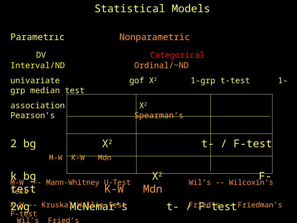
Statistical Models

Parametric Nonparametric

DV Categorical Interval/ND Ordinal/~ND

univariate gof X2 1-grp t-test 1-grp median test

association X2 Pearson’s Spearman’s

2 bg X2 t- / F-test M-W K-W Mdn

k bg X2 F-test K-W Mdn

2wg McNemar’s t- / F-test Wil’s Fried’s

kwg Cochran’s F-test Fried’s

M-W -- Mann-Whitney U-Test Wil’s -- Wilcoxin’s Test

K-W -- Kruskal-Wallis Test Fried’s -- Friedman’s F-test

Mdn -- Median Test

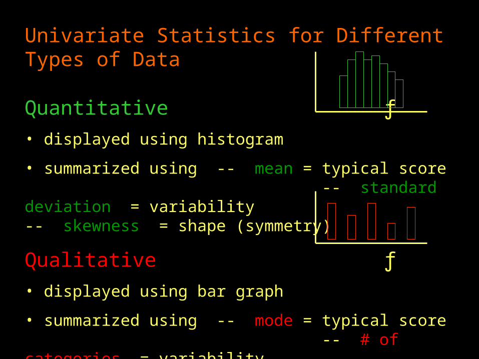
Univariate Statistics for Different Types of Data

Quantitative ƒ

• displayed using histogram

• summarized using -- mean = typical score -- standard deviation = variability -- skewness = shape (symmetry)

Qualitative ƒ

• displayed using bar graph

• summarized using -- mode = typical score -- # of categories = variability

Binary -- either as quant or as qual (be consistent)

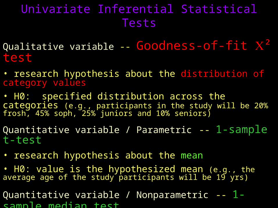
Univariate Inferential Statistical Tests

Qualitative variable -- Goodness-of-fit ² test• research hypothesis about the distribution of category values

• H0: specified distribution across the categories (e.g., participants in the study will be 20% frosh, 45% soph, 25% juniors and 10% seniors)

Quantitative variable / Parametric -- 1-sample t-test• research hypothesis about the mean

• H0: value is the hypothesized mean (e.g., the average age of the study participants will be 19 yrs)

Quantitative variable / Nonparametric -- 1-sample median test

• research hypothesis about the median

• H0: value is the hypothesized mean (e.g., the median age of the study participants will be 19 yrs)

• split sample at H0: median and run gof X2 w/ 50% & 50%

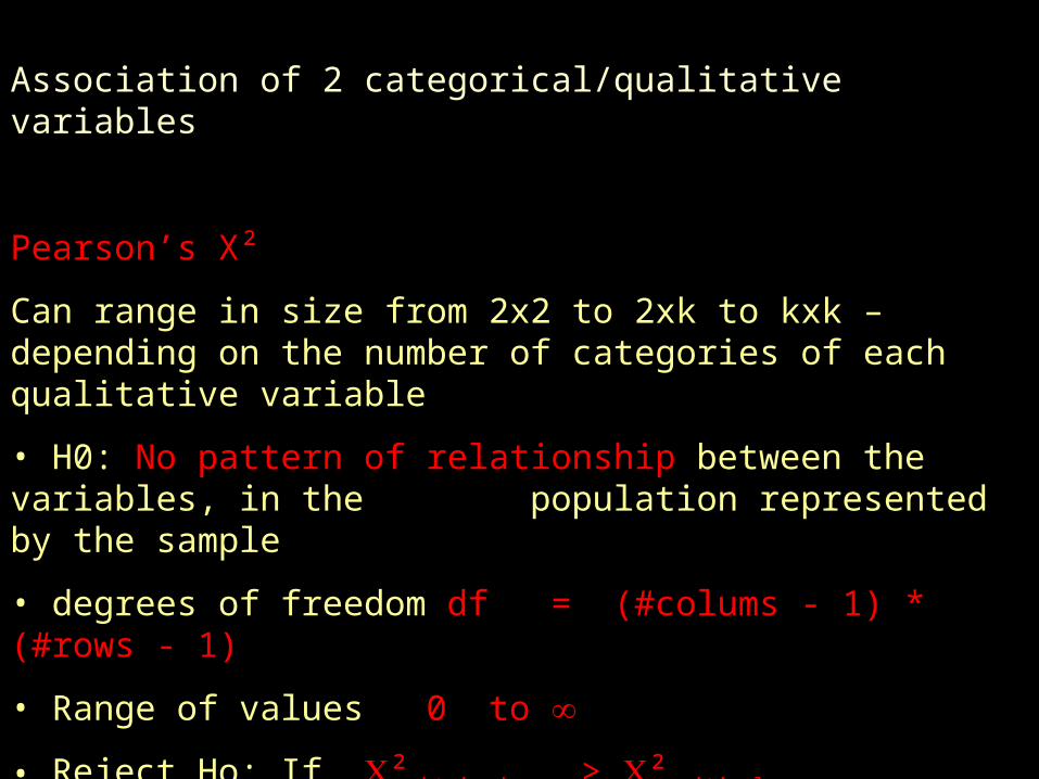
Association of 2 categorical/qualitative variables

Pearson’s X²

Can range in size from 2x2 to 2xk to kxk – depending on the number of categories of each qualitative variable

• H0: No pattern of relationship between the variables, in the population represented by the sample

• degrees of freedom df = (#colums - 1) * (#rows - 1)

• Range of values 0 to

• Reject Ho: If ²obtained > ²critical

Association of 2 quant variables / Parametric

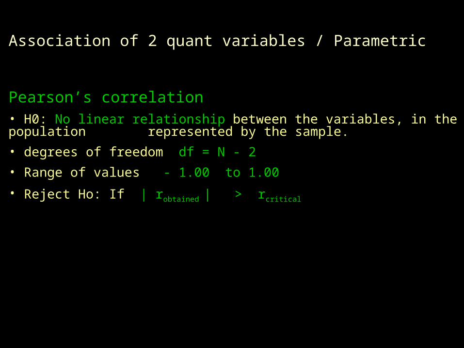
Pearson’s correlation• H0: No linear relationship between the variables, in the population

represented by the sample.

• degrees of freedom df = N - 2

• Range of values - 1.00 to 1.00

• Reject Ho: If | robtained | > rcritical

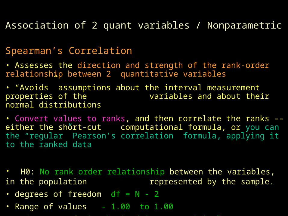
Association of 2 quant variables / Nonparametric

Spearman’s Correlation

• Assesses the direction and strength of the rank-order relationship between 2 quantitative variables

• “Avoids” assumptions about the interval measurement properties of the variables and about their normal distributions

• Convert values to ranks, and then correlate the ranks -- either the short-cut computational formula, or you can the “regular” Pearson’s correlation formula, applying it to the ranked data

• H0: No rank order relationship between the variables, in the population represented by the sample.

• degrees of freedom df = N - 2

• Range of values - 1.00 to 1.00

• Reject Ho: If | robtained | > rcritical

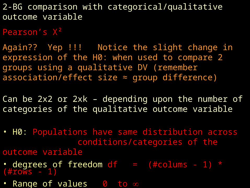
2-BG comparison with categorical/qualitative outcome variable

Pearson’s X²

Again?? Yep !!! Notice the slight change in expression of the H0: when used to compare 2 groups using a qualitative DV (remember association/effect size ≈ group difference)

Can be 2x2 or 2xk – depending upon the number of categories of the qualitative outcome variable

• H0: Populations have same distribution across conditions/categories of the outcome variable

• degrees of freedom df = (#colums - 1) * (#rows - 1)• Range of values 0 to • Reject Ho: If ²obtained > ²critical

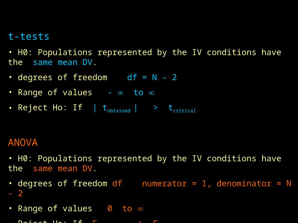
t-tests

• H0: Populations represented by the IV conditions have the same mean DV.

• degrees of freedom df = N - 2

• Range of values - to

• Reject Ho: If | tobtained | > tcritical

ANOVA

• H0: Populations represented by the IV conditions have the same mean DV.

• degrees of freedom df numerator = 1, denominator = N - 2

• Range of values 0 to

• Reject Ho: If Fobtained > Fcritical

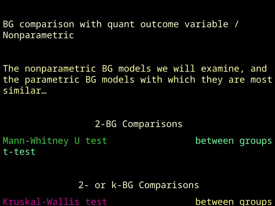
BG comparison with quant outcome variable / Nonparametric

The nonparametric BG models we will examine, and the parametric BG models with which they are most similar…

2-BG Comparisons

Mann-Whitney U test between groups t-test

2- or k-BG Comparisons

Kruskal-Wallis test between groups ANOVA

Median test between groups ANOVA

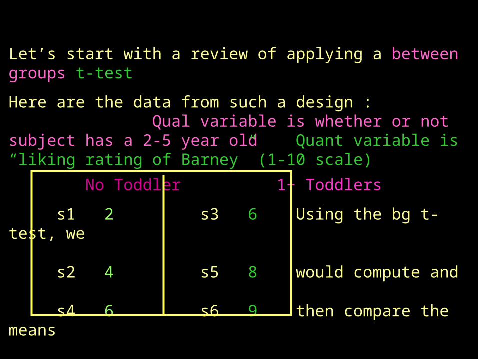
Let’s start with a review of applying a between groups t-test

Here are the data from such a design : Qual variable is whether or not subject has a 2-5 year oldQuant variable is “liking rating of Barney” (1-10 scale)

No Toddlertoddler 1+ Toddlers

s1 2 s3 6 Using the bg t-test, we

s2 4 s5 8 would compute and

s4 6 s6 9 then compare the means

s8 7 s7 10 of each group.

M = 4.75 M = 8.25

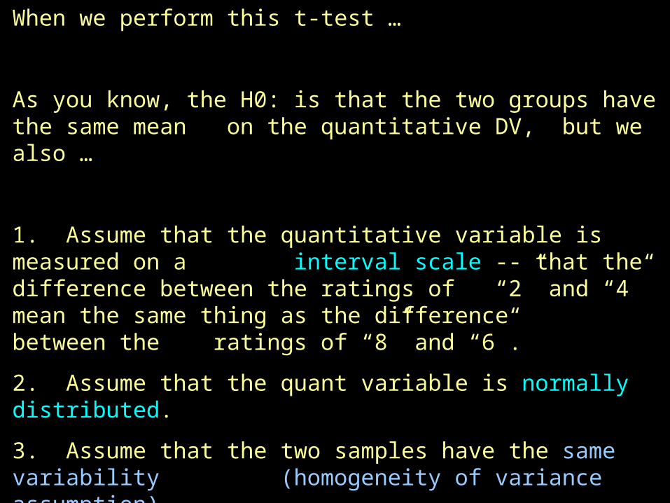
When we perform this t-test …

As you know, the H0: is that the two groups have the same mean on the quantitative DV, but we also …

1. Assume that the quantitative variable is measured on a interval scale -- that the difference between the ratings of “2” and “4” mean the same thing as the difference between the ratings of “8” and “6”.

2. Assume that the quant variable is normally distributed.

3. Assume that the two samples have the same variability (homogeneity of variance assumption)

Given these assumptions, we can use a t-test tp assess the H0: M1 = M2

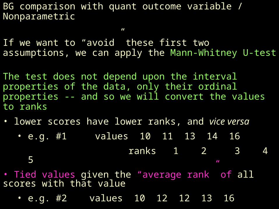
BG comparison with quant outcome variable / Nonparametric

If we want to “avoid” these first two assumptions, we can apply the Mann-Whitney U-test

The test does not depend upon the interval properties of the data, only their ordinal properties -- and so we will convert the values to ranks

• lower scores have lower ranks, and vice versa

• e.g. #1 values 10 11 13 14 16

ranks 1 2 3 4 5

• Tied values given the “average rank” of all scores with that value

• e.g. #2 values 10 12 12 13 16

ranks 1 2.5 2.5 4 5

• e.g., #3 values 9 12 13 13 13

ranks 1 2 4 4 4

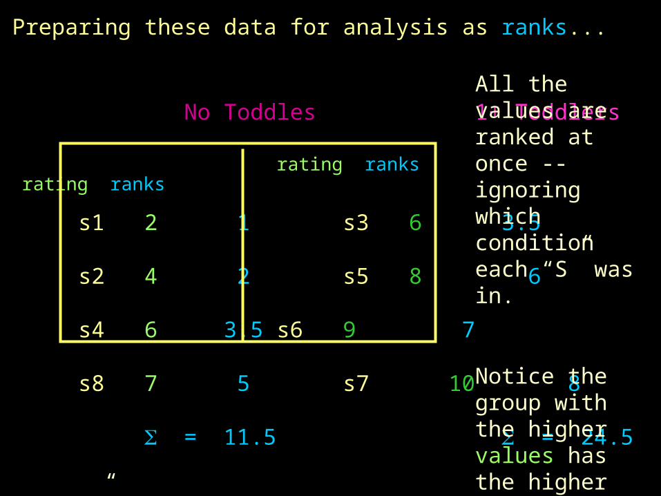
Preparing these data for analysis as ranks...

No Toddlestoddler 1+ Toddlers

rating ranks rating ranks

s1 2 1 s3 6 3.5

s2 4 2 s5 8 6

s4 6 3.5 s6 9 7

s8 7 5 s7 10 8

= 11.5 = 24.5

The “U” statistic is computed from the summed ranks. U=0 when the summed ranks for the two groups are the same (H0:)

All the values are ranked at once -- ignoring which condition each “S” was in.

Notice the group with the higher values has the higher summed ranks

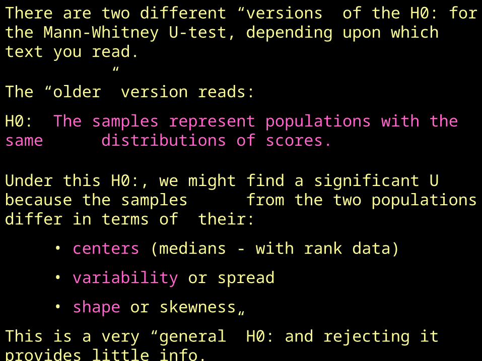
There are two different “versions” of the H0: for the Mann-Whitney U-test, depending upon which text you read.

The “older” version reads:

H0: The samples represent populations with the same distributions of scores.

Under this H0:, we might find a significant U because the samples from the two populations differ in terms of their:

• centers (medians - with rank data)

• variability or spread

• shape or skewness

This is a very “general” H0: and rejecting it provides little info.

Also, this H0: is not strongly parallel to that of the t-test (which is specifically about mean differences)

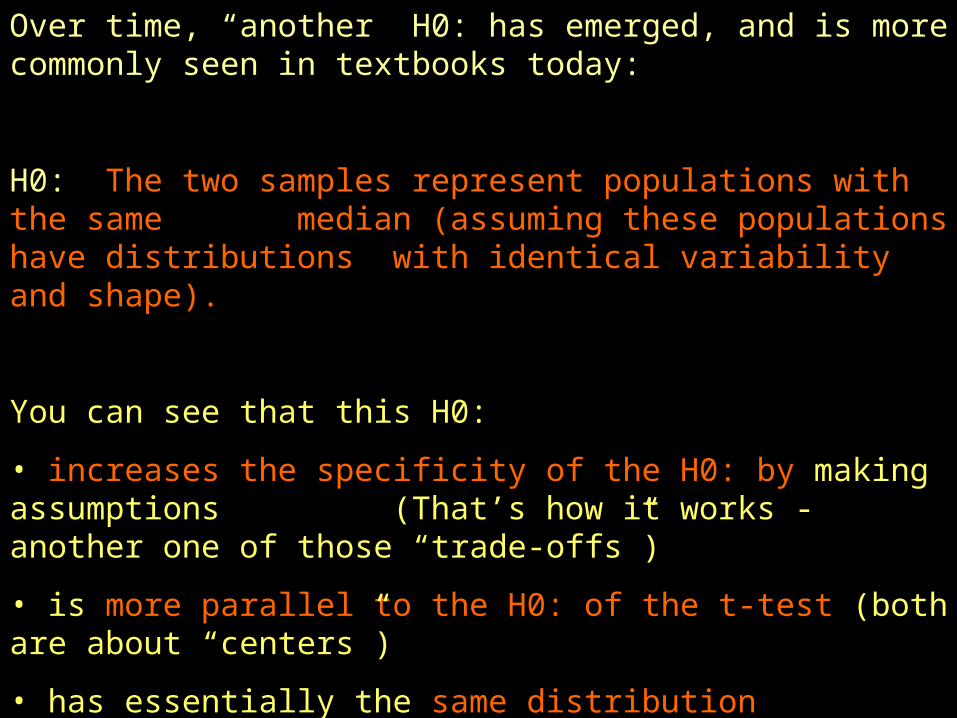
Over time, “another” H0: has emerged, and is more commonly seen in textbooks today:

H0: The two samples represent populations with the same median (assuming these populations have distributions with identical variability and shape).

You can see that this H0:

• increases the specificity of the H0: by making assumptions (That’s how it works - another one of those “trade-offs”)

• is more parallel to the H0: of the t-test (both are about “centers”)

• has essentially the same distribution assumptions as the t-test(equal variability and shape)

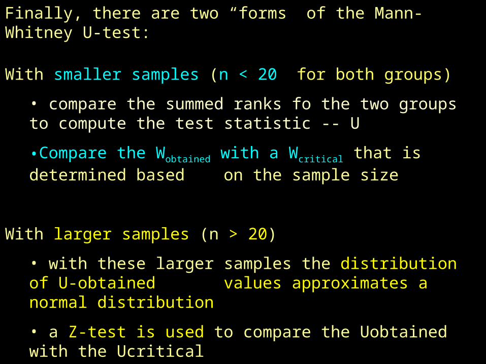
Finally, there are two “forms” of the Mann-Whitney U-test:

With smaller samples (n < 20 for both groups)

• compare the summed ranks fo the two groups to compute the test statistic -- U

•Compare the Wobtained with a Wcritical that is determined based on the sample size

With larger samples (n > 20)

• with these larger samples the distribution of U-obtained values approximates a normal distribution

• a Z-test is used to compare the Uobtained with the Ucritical

• the Zobtained is compared to a critical value of 1.96 (p = .05)

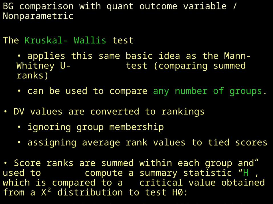
BG comparison with quant outcome variable / Nonparametric

The Kruskal- Wallis test

• applies this same basic idea as the Mann-Whitney U-test (comparing summed ranks)

• can be used to compare any number of groups.

• DV values are converted to rankings

• ignoring group membership

• assigning average rank values to tied scores

• Score ranks are summed within each group and used to compute a summary statistic “H”, which is compared to a critical value obtained from a X² distribution to test H0:

• groups with higher values will have higher summed ranks

• if the groups have about the same values, they will have about the same summed ranks

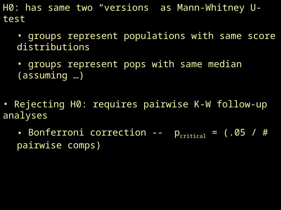
H0: has same two “versions” as Mann-Whitney U-test

• groups represent populations with same score distributions

• groups represent pops with same median (assuming …)

• Rejecting H0: requires pairwise K-W follow-up analyses

• Bonferroni correction -- pcritical = (.05 / # pairwise comps)

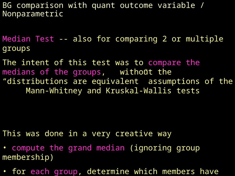
BG comparison with quant outcome variable / Nonparametric

Median Test -- also for comparing 2 or multiple groups

The intent of this test was to compare the medians of the groups, without the “distributions are equivalent” assumptions of the Mann-Whitney and Kruskal-Wallis tests

This was done in a very creative way

• compute the grand median (ignoring group membership)

• for each group, determine which members have scores above the grand median, and which have scores below the grand median

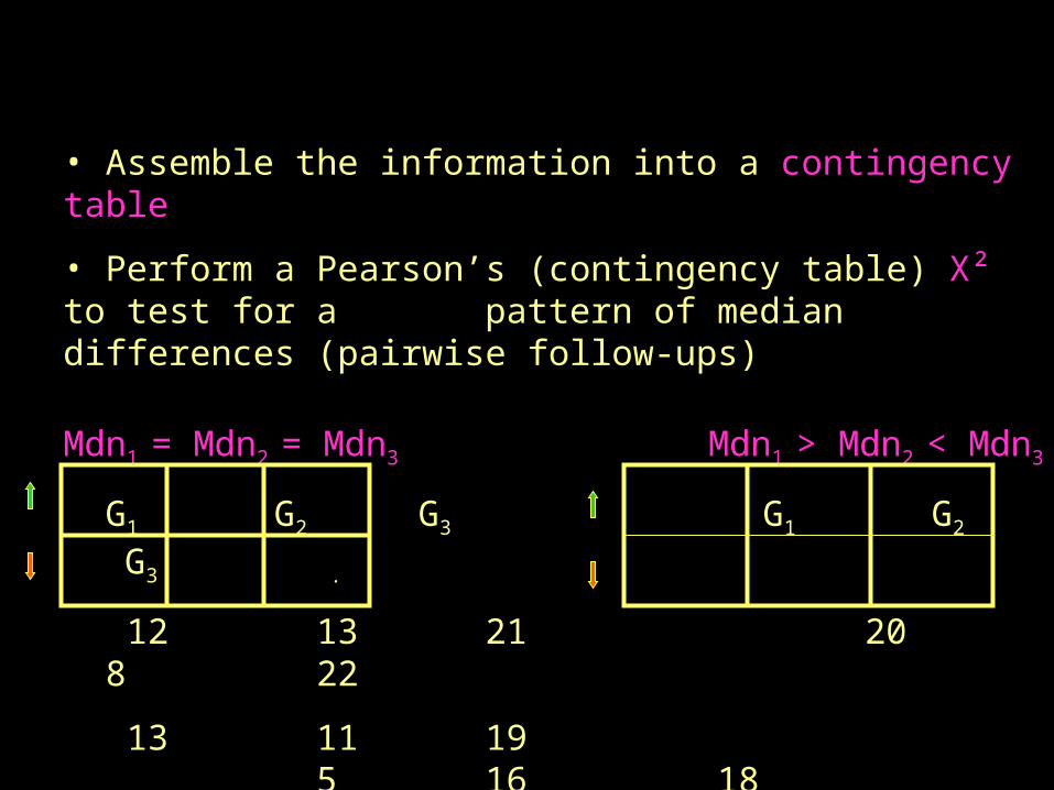
• Assemble the information into a contingency table

• Perform a Pearson’s (contingency table) X² to test for a pattern of median differences (pairwise follow-ups)

Mdn1 = Mdn2 = Mdn3 Mdn1 > Mdn2 < Mdn3

G1 G2 G3 G1 G2 G3 .

12 13 21 20 8 22

13 11 19 5 16 18

X² = 0 X² > 0