In 1999, the unique scientific opportunity to add intothe so-called A-train a POLDER designed instrument[1] onboard a CNES Myriade microsatellite [2] wasidentified. Thanks to its unique capability to performmultiangular and polarized acquisitions combinedwith the spectral information, PARASOL (Polariza-tion & Anisotropy of Reflectance for Atmospheric Sci-ences coupled with Observations from a Lidar) is ableto characterize the radiative properties of clouds andaerosols. In addition, the complementarity with othersensors flying in the A-train formation opens a largewindow of possibilities combining the various sets ofacquisitions from CERES and MODIS radiometers,the lidar on CALIPSO, and the radar on CLOUDSAT.
This “afternoon constellation” provides a unique at-mospheric observatory for aerosol and clouds charac-terization fundamental for a better knowledge oftheir radiative impact and to improve our under-standing of climate and climate change.
Table 1, the PARASOL payload, is a heritage ofPOLDER instruments [1] carried onboard ADEOS 1and 2 in 1996–1997 and 2002–2003. This innovativeconcept is a combination of polarization and multidi-rectional acquisitions: a complete description of thepolarization is available for 3 spectral bands and forup to 16 viewing angles. As shown in Table 2, thespectral signature of the target is assessed for 9 spec-tral bands in the 443–1020 nm spectral range. Foreach of the polarized bands, 490, 670, or 865, threeacquisitions are performed through a polarizer ori-ented with �60°, 0°, and 60° respectively from agiven reference, from which are retrieved the Stokesparameters [I, Q, U]. The major modification made on
the instrument compared to POLDER 1 and 2 was a90° rotation of the CCD matrix allowing PARASOL toperform more acquisitions along-track to enhance thecharacterization of the bidirectionality of targets. Asa result, the swath is reduced to 1600 km cross track(Table 1) compared to 2200 km for POLDER 1 and 2.
PARASOL was launched 18 December 2004, andthe first image was acquired 7 January 2005. Thecommissioning phase started with 2 months of spe-cific programming of both payload and satellite forcalibration and image quality purposes and missionstandard acquisitions started on 4 March 2005. Thecommissioning phase ended 12 July 2005 with theimage quality review. After one year of operationaluse, a general review was made confirming the ex-cellent health and performances of the PARASOLsystem [3]. A reprocessing of the level-1 archive,which included a correction of a light temporal de-crease of the radiometric sensitivity, was performedthe end of 2006.
The goal of this paper is an overview of results fromcalibration algorithms, characterization methods, andperformances for both geometric and radiometric as-pects. Because most of methods were previously de-scribed in other papers, mainly in Hagolle et al. [4]for radiometric aspects applied to the POLDER�ADEOS-1 sensor, the present paper does not detaileach algorithm but only provides brief descriptionsand focuses on particularity or innovative adapta-tions for PARASOL.
2. Radiometric Calibration and Performance
A. Preflight Characterization
For a given spectral band k, the radiometric model(simplified version including polarization) describesthe physical response of the instrument to the incom-ing signal characterized by [I, Q, U] in the Stokes’sformalism [5]. It can be written
Y l, p are the pixel coordinates,Y Xl,p is the numerical count measured for pixel
�l, p�,Y Cl,p is the dark current for pixel (l, p),Y �I, Q, U� are Stokes parameters expressed on a
given reference axis,Y Ak is the absolute calibration coefficient,Y G is the electronic gain,Y ti is the integration time,Y Pl,p is the low-frequency polynomial,Y gl,p is the high-frequency interpixel coefficient,
and where p1, p2, and p3 are depending on pixel coor-dinates, l and p, the optic sensitivity to polarization,�, and for polarized channels a the polarizer extinc-tion ratio, �, orientation, �a, and transmission, Ta.This radiometric model, its inversion to retrieve�I, Q, U�, and the full level-1 data processing are pre-cisely described in Hagolle et al. [5]. The preflightradiometric calibration of the instrument consists inaccurate estimation of each of these parameters. Pro-cedures and ground equipments are described in Ref.6, and some processing algorithms were improvedand updated in Ref. 7. Parameters are usually clas-sified into the following families:
Y Absolute calibration is the estimation of Ak,a global parameter independent of the consideredpixel.
Y In-polarization calibration refers to estimationof optic and polarizer sensitivity, i.e., estimation of Ta,�, �, and �a parameters.
Y Multiangular calibration refers for each spectralband to variation of the calibration with viewing angle
Table 1. Main Characteristics for PARASOL Satellite and Payload
Launch date 18th December 2004Platform MyriadAltitude 705 kmLocal time 13h30Mass 120 kgSize 0.6 � 0.8 � 0.8 mInstrument POLDERSpectral bands 9Polarized bands 3Spectral range 443–1020 nmDetector CCD Matrix 242 � 274Swath 1600 km cross-track
2100 km along-trackResolution 6.18 km (level-1 grid)Field-of-view �57°
Table 2. PARASOL Spectral Bands Including Central Wavelength, Bandwidth, Ability to Measure Polarization, and Saturation Level in ReflectanceUnit
or pixel, i.e., estimation of gl,p and Pl,p (when speakingabout equalization, Cl,p is also considered). Qualita-tively, the polynomial Pl,p refers to low-frequency vari-ations of the optic transmission slightly decreasingwhen the viewing angle is increasing, while the coef-ficient gl,p mainly refers to high-frequency variations ofthe sensitivity of elementary detectors or to variationsof the optic transmission that cannot be modeled as apolynomial function. These aspects are detailed forwide field-of-view sensors similar to PARASOL in Ref.4 (POLDER) and Ref. 8 (Végétation).
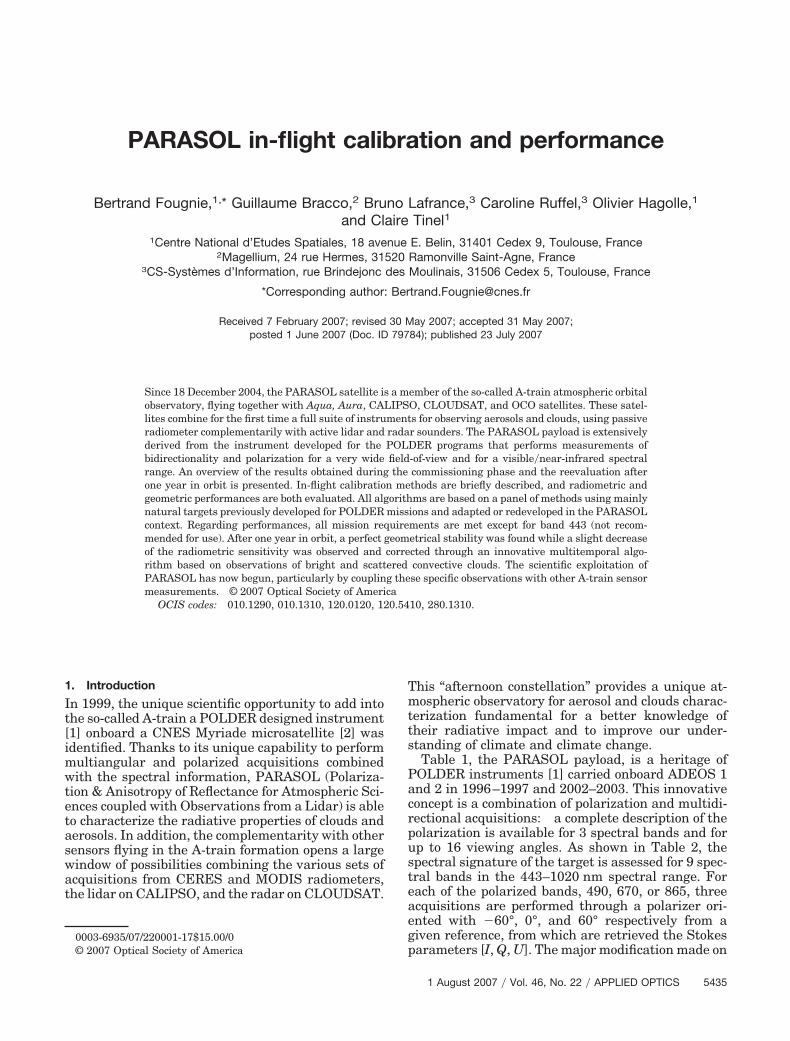
Figure 1 illustrates typical values for Pl,p (or P���) and����: Pl,p varies from 1 for nadir viewing to 0.88 atlarge viewing angles of 55°, i.e., a 12% decrease of thesensitivity, while ���� varies from 0 at nadir to about4% at 55°. Multiangular gl,p coefficients vary from0.98 to 1.02 over the matrix for which the mean valueis 1.0.
A full characterization of the spectral response ofthe instrument (hereafter called SRI) is required inorder to guarantee the efficiency of in-flight calibra-tion methods, but also to guarantee an optimizedscientific analysis over Earth–atmosphere targetsbehaving strongly differing spectral signatures asshown in Fig. 2. As no in-flight adjustment of the SRIwill be possible, various aspects of the SRI were an-alyzed with appropriate preflight sets of measure-ment: variability of the SRI into the field-of-view(typically 0.2 nm), spectral rejection (about 0.2%),variability over a given polarized triplet (better than�0.2 nm), and expected variation in the space vac-uum environment (less than 0.2 nm). The mean SRIsderived from the preflight campaign are given inTable 2.
As described in Fougnie et al. [9], a light nonlin-earity of the detector response was identified, mod-
eled as a function and corrected in the level-1processing. The preflight characterization of thisfunction is done using several acquisitions of thesame source for a great number of integration times.This nonlinearity function is illustrated Fig. 9 show-ing that neglect this correction would lead to �1%error on the retrieved normalized radiance I.
PARASOL is an instrument composed of a singlewide field-of-view camera [1]. Such instrumental con-cepts are usually concerned by stray-light phenom-ena. A stray-light correction, described in Ref. 5 orRef. 10 and included on the PARASOL level-1 pro-cessing algorithm, requires a dedicated characteriza-tion though a heavy preflight calibration campaign.A serious problem appeared for the band 443 forwhich it is supposed that a default occurred specifi-cally for this spectral band on the antireflect coatingof one of the several diopters composing the filter-wheel. Consequently, the stray-light intensity wasfound to be 5 to 10 times greater than other spectralbands and the correction algorithm on level-1 pro-cessing failed: unfortunately, the band 443 is withpoor accuracy. It is recommended to PARASOL datausers not to use this spectral band and we will discussno more the case of the band 443 in the following ofthis paper.
B. Absolute Calibration
1. Description of MethodsThe POLDER instrument has no on-board calibrationdevice to transfer-to-orbit the preflight calibration. Butnevertheless, even if the space sensor is able to deliveran autonomous on-board calibration, it has to be val-idated and controlled through vicarious methods; seeexamples in Eplee et al. [11] for SeaWiFs, Hagolleet al. [12] for MERIS, or Fougnie et al. [13] andHagolle et al. [4] for POLDER-1. Consequently, in-
Fig. 1. (Color online) Typical shapes and values for the polyno-mial P��� or Pl,p and epsilon ���� as a function of the viewing angle�. Polynomial P��� is linked to Pl,p through tan��� � �1�f�sqrt��l� 137.5�dl � �p � 121.5�dp� with f � 3.55 mm is the focal distanceof the instrument, dl � 32 and dp � 27 micrometers are sizes of aCCD pixel, l and p are CCD line and column numbers. For thenadir direction, P��� is normalized to 1 and ���� is null.
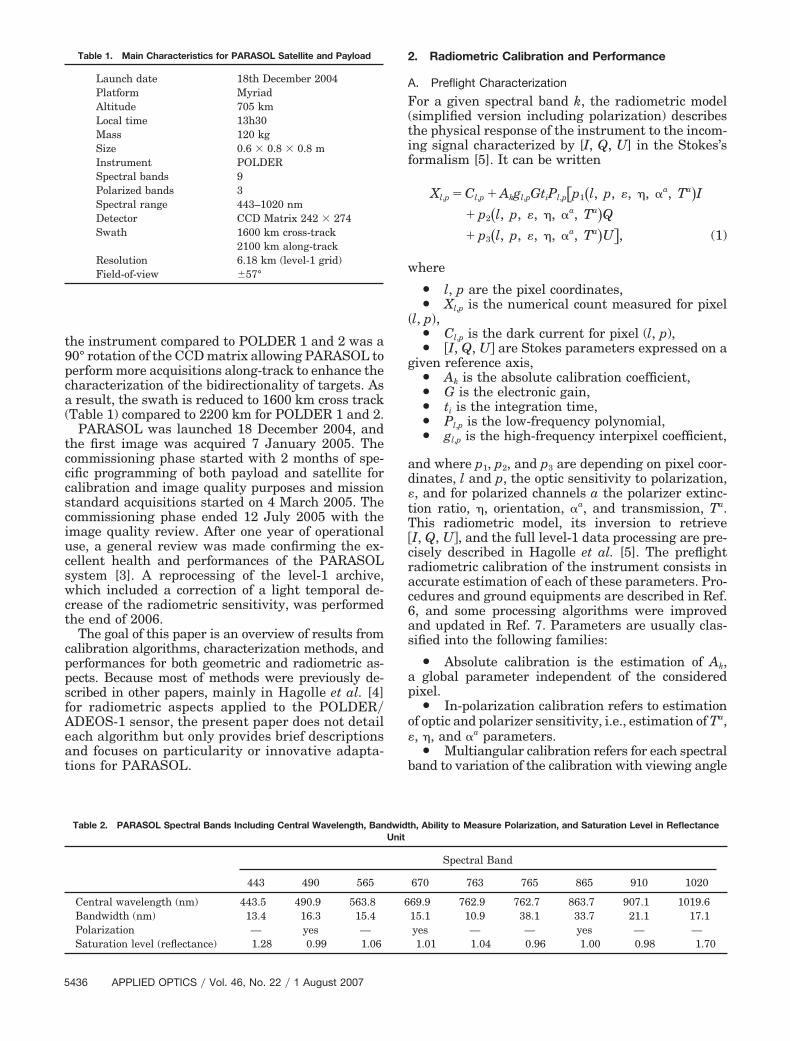
Fig. 2. Typical top-of-atmosphere normalized radiances for thePARASOL spectral bands and corresponding to targets selected forcalibration over Rayleigh scattering, sunglint, clouds, and desertsites. TOA normalized radiances, presented after gaseous absorp-tion correction for ozone, oxygen, and water vapor, illustrate dif-ferences between the various calibration targets for both spectralbehavior and radiance level aspects.
tensive efforts have historically been made to developcalibration methods based on acquisitions over nat-ural targets. Four particular natural targets from theEarth–atmosphere system were privileged for theirspecific characteristics. In such methods, the ap-proach is first to accurately compute the top-of-atmosphere (TOA) reference signal that the sensor ofinterest should observe over a selected target andsecondly, to compare the reference signal to the sig-nal really observed and delivered by the satellite sen-sor. These methods are:
(a) Absolute calibration over Rayleigh scattering:The TOA signal measured over oceanic sites, i.e.,dark surface, is due at 90% to scattering by atmo-spheric molecules, and this is the reason why thespectral behavior of the TOA signal is strongly vary-ing with the wavelength , very closely to a �4 law(see Fig. 2). In order to accurately compute this dom-inant Rayleigh scattering contribution, the equiva-lent Rayleigh optical thickness has to be calculatedfor each spectral band using surface pressure and theSRI (see, e.g., Ref. 13). Nevertheless, an absolute cal-ibration can be derived only if other contributors tothe TOA signal are controlled: clouds, aerosols, gas-eous absorption, surface phenomena, and marine re-flectances. Oligotrophic oceanic sites, illustrated onFig. 3, were selected for their homogeneities andmoderated seasonal variations, and were character-ized through a climatology of marine reflectance [14].Cloud and aerosol masks are based on a strict thresh-old using the band 865. A correction of the residualaerosol content is made assuming a Maritime-98%aerosol model from Shettle and Fenn [15] and usingthe background aerosol optical thickness measuredby the band 865 with a typical mean value of 0.025.This method used to calibrate spectral bands up to
670 nm is originally derived from Vermote et al. [16]and is described in Hagolle et al. [4].
(b) Interband calibration over sunglint: The reflex-ion of the sun over the oceanic surface observedfrom space is a bright and nearly spectrally whitephenomenon as illustrated in Fig. 2. An absolutecalibration over sunglint should require an accu-rate modeling of the sunglint radiance which isstrongly dependent on the sea surface roughness(as described by Cox and Munk [17] and in practicetoo difficult to assess. In fact, the white spectralbehavior shown in Fig. 2 can be used to provide aninterband calibration by simply comparing the sig-nal measured in various spectral bands to the sig-nal measured in a band used as reference. Somecorrections are nevertheless necessary: contribu-tion and transmission of molecular scattering, gas-eous absorption, marine reflectance (same oceanicsites defined Fig. 3 for Rayleigh scattering), andaerosol background. The multidirectional capabil-ity of PARASOL is used to efficiently discard mea-surements perturbed by aerosols using a thresholdon out-of-glint viewing direction. The referenceband to use should be well calibrated, and a redband (here 670 nm) is usually selected because oflower biases into the absolute calibration previ-ously derived from Rayleigh scattering method andlower atmospheric contribution than for shorterwavelengths. Another argument is that the intercali-bration error increases with spectral distance from thereference band, and the red band is at the middle of thespectral range of the instrument (see Table 2). Spectralbands from 490 to 1020 can be intercalibrated with theband 670. Principle of the method is described andapplied to POLDER-1 in Hagolle et al. [4], updated inHagolle et al. [18] in the case of VEGETATION, and ap-
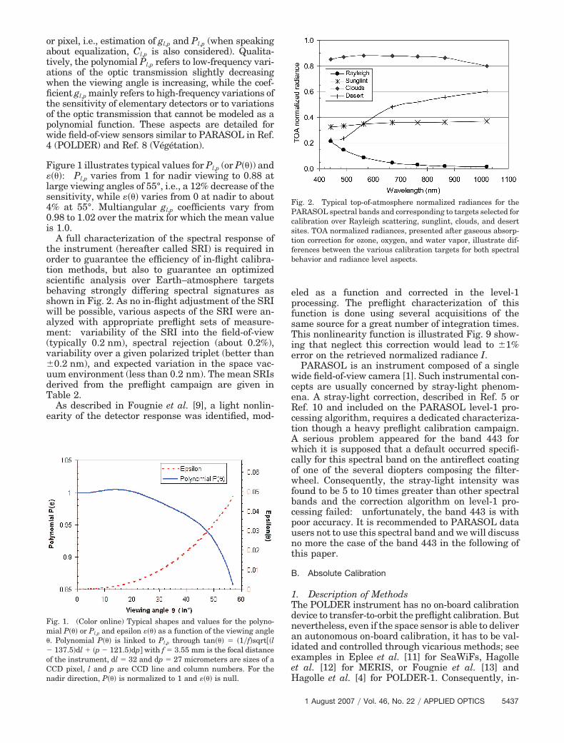
Fig. 3. (Color online) Location of calibration sites: oceanic sites used for Rayleigh scattering and sunglint calibrations (Indian, North�South Pacific, and Atlantic), oceanic sites used for calibration over bright clouds (Maldives and Guinea), desert sites used for crosscalibration with other sensors (20 sites in Africa and Arabia), and Antarctic sites used for multitemporal calibration (4 sites in Dome C,not presented on this paper).
plied for calibration of POLDER polarized channel inToubbé et al. [19].
(c) Interband calibration over clouds: High anddense convective clouds are strongly reflecting thedownwelling irradiance of the sun, and such cloudscan be assumed white and Lambertian with a verygood approximation as illustrated in Fig. 2. Using aspectral band as reference to characterize the reflec-tance of the cloud (a red band as for sunglint), it istherefore possible to derive an interband calibration.Candidate observations are selected using severalcriteria: privileged oceanic sites known for theiradapted convective dynamics (Fig. 3), very high re-flectance level characterizing a strong scattered cloud(up to 0.7), small apparent pressure deducted fromthe 763�765 ratio [20] assuring a very high altitude ofthe cloud (less than 400 hPa), and specific viewingconditions for reduced geometric effects (solar andviewing zenith angles less than 40°). Gaseous absorp-tion and correction of the Rayleigh contribution abovethe cloud is considered. The algorithm includes amultilayer decomposition of the atmosphere and aconsideration of the microphysics of the cloud parti-cles: hexagonal columns, plates, or compact hexag-onal crystals with a moderated impact on results (1 to2% depending on wavelength) [21]. Using the redband as reference (as for sunglint), bands from 490 to865 can be intercalibrated. This method is fully de-scribed in Lafrance et al. [21], including the cloudmicrophysics consideration, i.e., cloud particle type,and applied to POLDER-1 in Hagolle et al. [4].
(d) Cross calibration over desert sites: Desert sitesrepresent remarkably stable targets for which it ispossible to perform multitemporal survey and crosscalibration with other sensors. 20 desert sites of100 100 km2, and located in Africa and Arabia (seeFig. 3), were selected for their properties, mainly ho-mogeneity and stability with time [22]. In addition,this temporal stability of such sites can be used tocross calibrate different sensors for which viewinggeometries are different [23]. The algorithm re-searches similar viewing geometries between acqui-sitions of a given sensor to calibrate and an archive ofacquisitions made by a sensor used as reference. Thenumber of such coincidence can be sensitively in-creased when considering reciprocal viewing condi-tions [23]. Firstly, leaving from the TOA signalmeasured by the reference sensor, an appropriateatmospheric correction is made considering molecu-lar and aerosol contributions (desertic aerosol modelwith an optical thickness of 0.2). A spectral interpo-lation of the surface reflectance deducted from thereference sensor measurements is made to computethe surface reflectance observed by the sensor to becalibrated weighted by its own instrumental re-sponse. Finally, the atmospheric contribution isadded to rebuild the TOA signal which is compared tothe TOA signal really measured by the sensor to cal-ibrate and for which a typical aspect is given Fig. 2.This algorithm using acquisitions over 20 desert sites
is described in Cabot et al. [23], applied to POLDER-1in Hagolle et al. [4], and used for ocean color multi-sensor cross calibration in Fougnie et al. [24].
For all these methods, gaseous corrections wereperformed using the SMAC approach described inRef. 25. Gaseous contributions were corrected usingexogenous data from meteorological products: ozonecontent, surface pressure (for oxygen correction, exceptfor calibration over high clouds for which the apparentpressure deducted from 763�765 is used according Ref.4) and water vapor content.
2. Calibration ResultsThe in-flight calibration of PARASOL was conductedin a similar way as for POLDER [4] or VEGETATION
[18] and described in Table 4. In this approach, theratio of measured radiance, MI, to calculated radi-ance, CI, computed using various methods is called�Ak because it can be interpreted as a calibrationerror on the analyzed data for the spectral band k.Firstly, an absolute calibration of shorter wave-lengths was made using Rayleigh scattering deriving�Ak
Ray�490�, �AkRay�565�, and �Ak
Ray�670�. Secondly,an interband calibration over sunglint using band670 as reference provided coefficients �Ak
Sun�NIR�� dAk�NIR� �Ak
Ray�670� for near infrared bands NIRwhere dAk�NIR� are interband calibration coefficientsand assuming dAk�670� � 1. The calibration oversunglint also evaluates �Ak
Sun�490� and �AkSun�565�
coefficients for shorter wavelengths. In order to avoida direct propagation of any bias uniquely due to erroron the knowledge of the real �Ak�670� to other longerwavelengths, a compromise is found adjusting previ-ous results with Fadj defined by
Fadj � ��AkRay�490� � �Ak
Ray�565� � �AkRay�670���
��AkSun�490� � �Ak
Sun�565� � �AkSun�670��.
(2)
Finally, “compromised” calibration coefficientsare defined by
Y �AkRay�490�, �Ak
Ray�565�, �AkRay�670� for visible
bands,Y �Ak
Sun�NIR� � Fadj dAk�NIR� �AkRay�670� for
NIR bands 765, 865, and 1020.
Note that in absolute calibration over Rayleighscattering, the band 865 used to correct the residualaerosol background need to be well calibrated. Con-sequently, if �Ak
Sun�865� is found to be sensitivelydifferent than 1.0, an iteration is required: the ab-solute calibration over Rayleigh scattering must berecomputed using MI�865���Ak
Sun�865� instead ofMI(865) to estimate the aerosol radiance, then theinterband calibration must be reappraised, and soon . . . Since a 5% error on band 865 leads to a 1%error on �Ak
Ray�490� [4,13], a good convergence is ob-served after one or 2 steps.
Results illustrated in Figs. 4–7 for bands 490, 670,and 865, and summarized in Table 3, are based on 3
months of PARASOL data from March until May2005. A strong adjustment from preflight calibrationwas necessary and the 4% to 9%, depending on thewavelength, were retrospectively explained by a bi-ased calibration of the integrating sphere used forPARASOL preflight absolute calibration. Results ob-tained using calibration over Rayleigh scattering(Fig. 4), interband over sunglint (Fig. 5) or over clouds(Fig. 6), and cross calibration with POLDER-2 (Fig. 7)show confident behavior when analyzed as a functionof the observed normalized radiance (as in Figs. 4–7)or other geometric or geophysical parameters. Figure8 and Table 3 point out the good global consistencybetween results for all the spectral range (except theband 443): results are within �1% for 490 and 670,�1.5% for 865, and �2% for 565, 765, and 1020. Sucha consistence from various calibration methods us-
ing four different targets corresponding to very dif-ferent spectral signatures and reflectance levels (asshown in Fig. 2), and very varied geometric condi-tions (viewing and solar), gives a good confidence onthe PARASOL level-1 calibration.
The calibration of the band 763, centered on theoxygen A-band absorption, can be derived from theabsolute calibration of the band 765, which was ad-justed by 7% (see Table 3). The method consists incomparing the O2 transmission obtained using sur-face pressure at the sea level in clear sky conditionsand the transmission derived from the differentialabsorption method using PARASOL observations atbands 763 and 765 [20]. As described in Ref. 4, ac-quisitions over sunglint are adequate for this calibra-tion. Results evidenced a necessary �2% adjustmenton the preflight interband calibration of bands 763
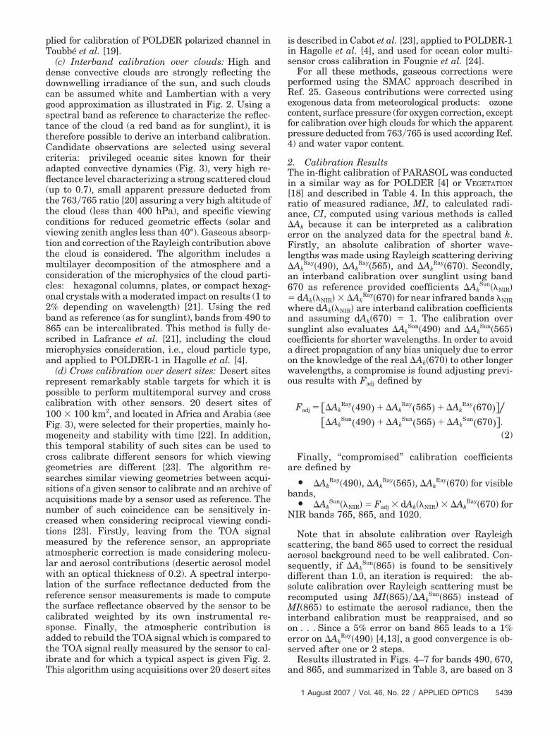
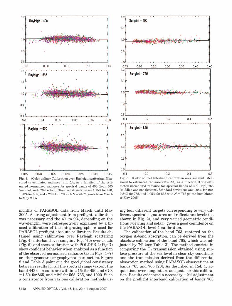
Fig. 4. (Color online) Calibration over Rayleigh scattering. Mea-sured to estimated radiance ratio �Ak as a function of the esti-mated normalized radiance for spectral bands of 490 (top), 565(middle), and 670 (bottom). Standard deviations are 1.15% for 490,1.38% for 565, and 2.29% for 670 with N � 4457 points from Marchto May 2005.
Fig. 5. (Color online) Interband calibration over sunglint. Mea-sured to estimated radiance ratio �Ak as a function of the esti-mated normalized radiance for spectral bands of 490 (top), 765(middle), and 865 (bottom). Standard deviations are 0.88% for 490,0.84% for 765, and 1.05% for 865 with N � 765 points from Marchto May 2005.
and 765 leading to an absolute adjustment for 763 of5% (Table 3). The band 910 is centered on a watervapor absorption peak. The same approach is usedthan for band 763, i.e., band 910 is intercalibratedwith band 865. This intercalibration between bands910 and 865 was kept to preflight calibration as it wasmade for previous POLDER 1 and 2 [4].
C. Multitemporal Monitoring
Evolution with time of the radiometric sensitivity ofthe instrument is a natural process. During the firstdays or months in orbit, some optical parts of the in-strument may have molecular outgassing phenomenain the vacuum of space. A more or less long-term effectevolution may be due to aging of the optical partsenduring “aggressive” solar irradiation. Several spacesensors are equipped with on-board device to monitor
possible temporal evolution. SeaWiFS [26], MERIS[27], or MODIS [28] are equipped with solar diffuserswhile VEGETATION�SPOT [18] is equipped with anonboard lamp. In all cases, difficulties are encoun-tered: aging of the lamp or diffuser themselvesmay occur requiring a complementary on-boardmonitoring through diffuser duplication for exam-ple [27,28]. Complementarily, the moon is used as anatural and external diffuser to monitor SeaWiFSlong-term trends using acquisitions for specific lunarphases [29]. Alternative methods using natural tar-gets from the Earth–atmosphere system were devel-oped: over desert sites [23,24], viewing sunglint [18]or over Antarctica [30]. Nevertheless, some limita-tions are due to perturbing contribution or inaccuracyon the algorithm, such as aerosol perturbation, sea-sonal effects, bidirectional effects, spectral behavior
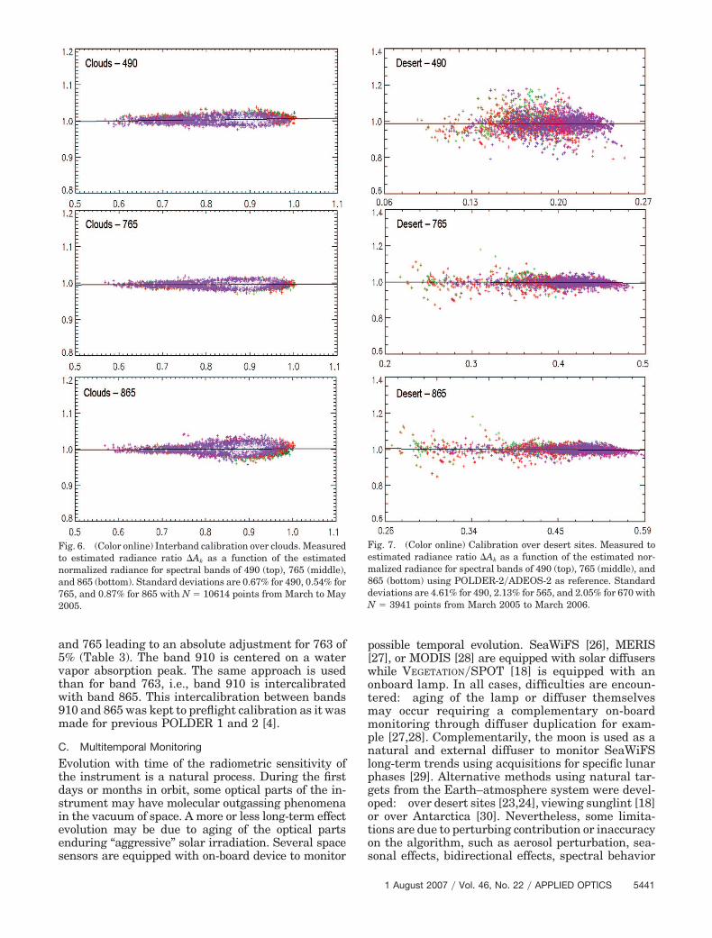
Fig. 6. (Color online) Interband calibration over clouds. Measuredto estimated radiance ratio �Ak as a function of the estimatednormalized radiance for spectral bands of 490 (top), 765 (middle),and 865 (bottom). Standard deviations are 0.67% for 490, 0.54% for765, and 0.87% for 865 with N � 10614 points from March to May2005.
Fig. 7. (Color online) Calibration over desert sites. Measured toestimated radiance ratio �Ak as a function of the estimated nor-malized radiance for spectral bands of 490 (top), 765 (middle), and865 (bottom) using POLDER-2�ADEOS-2 as reference. Standarddeviations are 4.61% for 490, 2.13% for 565, and 2.05% for 670 withN � 3941 points from March 2005 to March 2006.
modeling, or difficulty to obtain a dense temporalsampling.
PARASOL is not equipped with an onboard cali-bration device. After one year in orbit, it was evi-denced by all methods used to estimate the absolutecalibration (Subsection 2.B.1) that a temporal de-crease of the radiometric sensitivity occurred. It wasnecessary to choose the best reference as possible tomonitor the multitemporal decrease of the sensitiv-ity. Regarding theoretical error budgets for eachmethod [4,18,21,23,31], effective behaviors of results(bias and root mean square error), spectral shapes ofthe targets leading to potential errors into the model,and finally the temporal sampling, the calibrationover white convective clouds was preferred as thebest compromise. In addition, this reference is phys-ically very close to the white moon diffuser that pro-vided essential results for SeaWiFs [29].
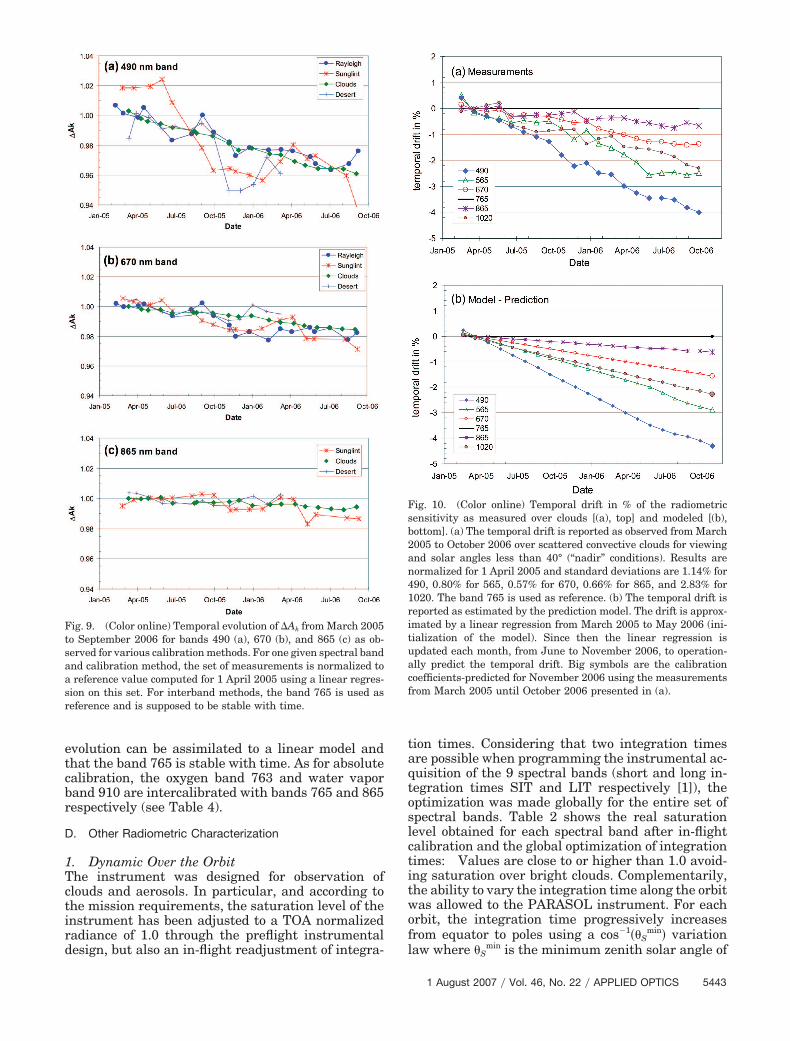
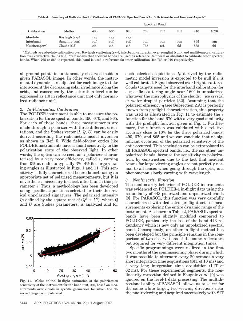
Figures 9(a)–9(c) measurements were analyzedover 18 months for the four calibration methods andfor bands 490, 670, and 865 separately. For interbandmethods, i.e., calibration over sunglint and clouds, atemporally stable reference was necessary to deriveresults presented in Fig. 9: The band 765 was se-lected as the best stable reference with time. This lasthypothesis is based on two arguments: First, inter-band results show that all the spectral bands aredecreasing more with time than band 765 [Fig. 10(a)].Second, when the band 765 is supposed stable, a verygood consistency is found with absolute calibrationover Rayleigh scattering and cross calibration overdesert sites, for all spectral bands (Fig. 9) includingthe band 765. A very good consistency is observed forred (670) to near-infrared (865) spectral bands: Thetemporal drift is found to be sensible for bands 490,670, and a very small for band 865. Results oversunglint or desert sites for the band 490 seem inac-curate with a strong dispersion as confirmed bytheoretical error budgets [18,23,31]. Multitemporalcalibration over Rayleigh scattering provides inter-esting confident results for bands 490 and 670, butthe best repeatability is observed for white convectiveclouds, confirming the adequation of such diffusers asexcellent references. Figures 9 and 10 show the an-nual mean drift can be estimated with an accuracywithin 0.5% per year. Figure 10(a), results of calibra-tion over clouds, are shown for all spectral bands(except gaseous and 443 bands). The temporal drift in% per year varies from �3% at 490 to �1% at 670, isnull for 765, and reached �1.5% for 1020. Exponen-tial functions are used for SeaWiFs [26] and MERIS[27] to model the temporal drift, but Fig. 10(a) showsthat a linear model is sufficient to describe thePARASOL evolution. The prediction model illustratedFig. 10(b) is based on a linear fit over the 15 firstmonths, from March 2005 until June 2006. SinceJuly 2006, the prediction model is used to opera-tionally predict the new calibration coefficient to beapplicable in the level-1 processing of the next month:for this, the linear regression is updated based on themeasurement dataset completed by the new mea-surement of the current month. A long term monitor-ing will deal with the two assumptions that the
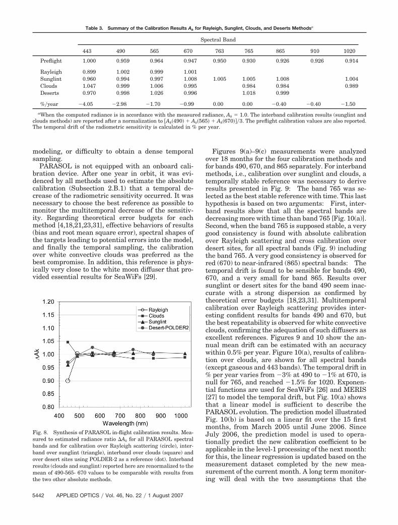
Table 3. Summary of the Calibration Results Ak for Rayleigh, Sunglint, Clouds, and Deserts Methodsa
aWhen the computed radiance is in accordance with the measured radiance, Ak � 1.0. The interband calibration results (sunglint andclouds methods) are reported after a normalization to �Ak�490� � Ak�565� � Ak�670���3. The preflight calibration values are also reported.The temporal drift of the radiometric sensitivity is calculated in % per year.
Fig. 8. Synthesis of PARASOL in-flight calibration results. Mea-sured to estimated radiance ratio �Ak for all PARASOL spectralbands and for calibration over Rayleigh scattering (circle), inter-band over sunglint (triangle), interband over clouds (square) andover desert sites using POLDER-2 as a reference (dot). Interbandresults (clouds and sunglint) reported here are renormalized to themean of 490-565- 670 values to be comparable with results fromthe two other absolute methods.
evolution can be assimilated to a linear model andthat the band 765 is stable with time. As for absolutecalibration, the oxygen band 763 and water vaporband 910 are intercalibrated with bands 765 and 865respectively (see Table 4).
D. Other Radiometric Characterization
1. Dynamic Over the OrbitThe instrument was designed for observation ofclouds and aerosols. In particular, and according tothe mission requirements, the saturation level of theinstrument has been adjusted to a TOA normalizedradiance of 1.0 through the preflight instrumentaldesign, but also an in-flight readjustment of integra-
tion times. Considering that two integration timesare possible when programming the instrumental ac-quisition of the 9 spectral bands (short and long in-tegration times SIT and LIT respectively [1]), theoptimization was made globally for the entire set ofspectral bands. Table 2 shows the real saturationlevel obtained for each spectral band after in-flightcalibration and the global optimization of integrationtimes: Values are close to or higher than 1.0 avoid-ing saturation over bright clouds. Complementarily,the ability to vary the integration time along the orbitwas allowed to the PARASOL instrument. For eachorbit, the integration time progressively increasesfrom equator to poles using a cos�1��S
min� variationlaw where �S
min is the minimum zenith solar angle of
Fig. 9. (Color online) Temporal evolution of �Ak from March 2005to September 2006 for bands 490 (a), 670 (b), and 865 (c) as ob-served for various calibration methods. For one given spectral bandand calibration method, the set of measurements is normalized toa reference value computed for 1 April 2005 using a linear regres-sion on this set. For interband methods, the band 765 is used asreference and is supposed to be stable with time.
Fig. 10. (Color online) Temporal drift in % of the radiometricsensitivity as measured over clouds [(a), top] and modeled [(b),bottom]. (a) The temporal drift is reported as observed from March2005 to October 2006 over scattered convective clouds for viewingand solar angles less than 40° (“nadir” conditions). Results arenormalized for 1 April 2005 and standard deviations are 1.14% for490, 0.80% for 565, 0.57% for 670, 0.66% for 865, and 2.83% for1020. The band 765 is used as reference. (b) The temporal drift isreported as estimated by the prediction model. The drift is approx-imated by a linear regression from March 2005 to May 2006 (ini-tialization of the model). Since then the linear regression isupdated each month, from June to November 2006, to operation-ally predict the temporal drift. Big symbols are the calibrationcoefficients-predicted for November 2006 using the measurementsfrom March 2005 until October 2006 presented in (a).
all ground points instantaneously observed inside agiven PARASOL image. In other words, the instru-mental dynamic is readjusted for each image to takeinto account the decreasing solar irradiance along theorbit, and consequently, the saturation level can beexpressed as 1.0 in reflectance unit (not only normal-ized radiance unit).
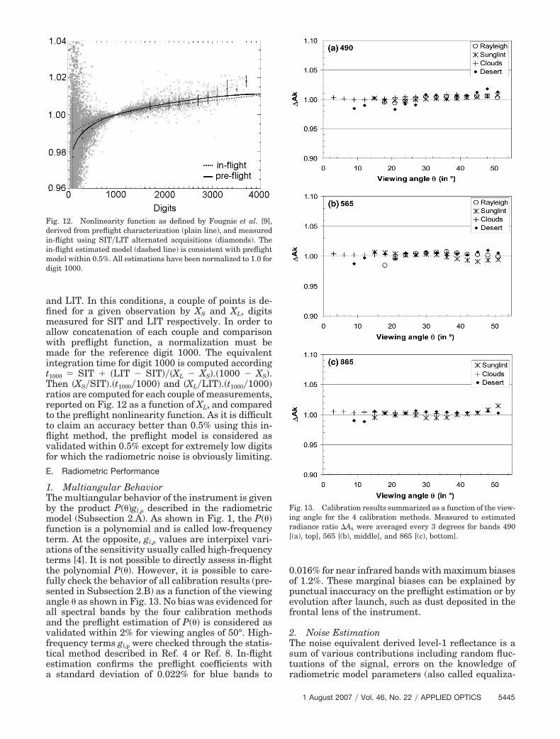
2. In-Polarization CalibrationThe POLDER instrument is able to measure the po-larization for three spectral bands, 490, 670, and 865.For each of these bands, three measurements aremade through a polarizer with three different orien-tations, and the Stokes vector [I, Q, U] can be easilyderived according the radiometric model inversionas shown in Ref. 5. Wide field-of-view optics likePOLDER instruments have a small sensitivity to thepolarization state of the observed light. In otherwords, the optics can be seen as a polarizer charac-terized by a very poor efficiency, called �, varyingfrom 0% at nadir to typically 3%–4% for large view-ing angles as illustrated in Figs. 1 and 11. This sen-sitivity is fully characterized before launch using anappropriate set of polarized measurements, but it isnevertheless necessary to check after launch this pa-rameter �. Thus, a methodology has been developedusing specific acquisitions selected for their theoret-ical unpolarized signatures. The polarized intensityIp defined by the square root of �Q2 � U2�, where Qand U are Stokes parameters, is analyzed and for
such selected acquisitions, Ip derived by the radio-metric model inversion is expected to be null if � iswell calibrated. Signal observed over bright scatteredclouds (targets used for the interband calibration) fora specific scattering angle near 160° is unpolarizedwhatever the microphysics of the clouds: ice crystalor water droplet particles [32]. Assuming that thepolarizer efficiency � (see Subsection 2.A) is perfectlyknown from preflight characterization, this propertywas used as illustrated in Fig. 11 to estimate the �function for the band 670 with a very good similaritywith the preflight function given in Fig. 1. Further-more, the � function was validated with a relativeaccuracy close to 10% for the three polarized bands,490, 670, and 865 and we can conclude that no sig-nificant evolution of the polarized sensitivity of theoptic occurred. This conclusion can be extrapolated toall PARASOL spectral bands, i.e., the six other un-polarized bands, because the sensitivity to polariza-tion, by construction due to the fact that incidentbeams for large viewing angles are not perfectly nor-mal to all lenses when going through the optic, is aphenomenon slowly varying with wavelength.
3. Nonlinearity FunctionThe nonlinearity behavior of POLDER instrumentswas evidenced on POLDER-1 in-flight data using theredundancy of 443 polarized and unpolarized bands[9]. For PARASOL, this function was very carefullycharacterized with dedicated preflight sets of mea-surements exploring the entire dynamic range of theinstrument. As shown in Table 2, PARASOL spectralbands have been slightly modified compared toPOLDER, particularly the loss of the band 443 re-dundancy which is now only an unpolarized spectralband. Consequently, an other in-flight method hasbeen developed but the principle remains in the com-parison of two observations of the same reflectancebut acquired for very different integration times.
Specific programmings were realized in the firsttwo months of the commissioning phase during whichit was possible to alternate every 20 seconds a veryshort integration time acquisitions (SIT of 10 ms) anda very long integration time acquisition (LIT of62 ms). For these experimental segments, the non-linearity correction defined in Fougnie et al. [9] wasignored on the level-1 data processing. The multidi-rectional ability of PARASOL allows us to select forthe same white target, two viewing directions nearthe nadir viewing and acquired successively with SIT
Table 4. Summary of Methods Used to Calibration all PARASOL Spectral Bands for Both Absolute and Temporal Aspectsa
Calibration Method
Spectral Band
490 565 670 763 765 865 910 1020
Absolute Rayleigh (ray) ray ray rayInterband Sunglint (sun) ref. ref. ref. sun sun sun 865 sunMultitemporal Clouds (cld) cld cld cld 765 ref. cld 865 cld
aMethods are absolute calibration over Rayleigh scattering (ray), interband calibration over sunglint (sun), and multitemporal calibra-tion over convective clouds (cld). “ref” means that spectral bands are used as reference (temporal or absolute) to calibrate other spectralbands. When 765 or 865 is reported, this band is used a reference for inter-calibration (for 763 or 910 respectively).
Fig. 11. (Color online) In-flight estimation of the polarizationsensitivity of the instrument for the band 670, �(�), based on mea-surements over clouds in specific geometries for which the ob-served target is unpolarized.
and LIT. In this conditions, a couple of points is de-fined for a given observation by XS and XL, digitsmeasured for SIT and LIT respectively. In order toallow concatenation of each couple and comparisonwith preflight function, a normalization must bemade for the reference digit 1000. The equivalentintegration time for digit 1000 is computed accordingt1000 � SIT � �LIT � SIT���XL � XS�.�1000 � XS�.Then �XS�SIT�.�t1000�1000� and �XL�LIT�.�t1000�1000�ratios are computed for each couple of measurements,reported on Fig. 12 as a function of XL, and comparedto the preflight nonlinearity function. As it is difficultto claim an accuracy better than 0.5% using this in-flight method, the preflight model is considered asvalidated within 0.5% except for extremely low digitsfor which the radiometric noise is obviously limiting.
E. Radiometric Performance
1. Multiangular BehaviorThe multiangular behavior of the instrument is givenby the product P���gl,p described in the radiometricmodel (Subsection 2.A). As shown in Fig. 1, the P���function is a polynomial and is called low-frequencyterm. At the opposite, gl,p values are interpixel vari-ations of the sensitivity usually called high-frequencyterms [4]. It is not possible to directly assess in-flightthe polynomial P���. However, it is possible to care-fully check the behavior of all calibration results (pre-sented in Subsection 2.B) as a function of the viewingangle � as shown in Fig. 13. No bias was evidenced forall spectral bands by the four calibration methodsand the preflight estimation of P��� is considered asvalidated within 2% for viewing angles of 50°. High-frequency terms gl,p were checked through the statis-tical method described in Ref. 4 or Ref. 8. In-flightestimation confirms the preflight coefficients witha standard deviation of 0.022% for blue bands to
0.016% for near infrared bands with maximum biasesof 1.2%. These marginal biases can be explained bypunctual inaccuracy on the preflight estimation or byevolution after launch, such as dust deposited in thefrontal lens of the instrument.
2. Noise EstimationThe noise equivalent derived level-1 reflectance is asum of various contributions including random fluc-tuations of the signal, errors on the knowledge ofradiometric model parameters (also called equaliza-
Fig. 12. Nonlinearity function as defined by Fougnie et al. [9],derived from preflight characterization (plain line), and measuredin-flight using SIT�LIT alternated acquisitions (diamonds). Thein-flight estimated model (dashed line) is consistent with preflightmodel within 0.5%. All estimations have been normalized to 1.0 fordigit 1000.
Fig. 13. Calibration results summarized as a function of the view-ing angle for the 4 calibration methods. Measured to estimatedradiance ratio �Ak were averaged every 3 degrees for bands 490[(a), top], 565 [(b), middle], and 865 [(c), bottom].
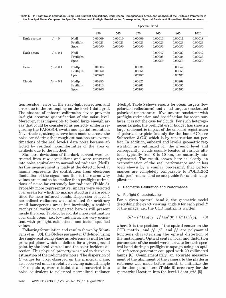
tion residue), error on the stray-light correction, anderror due to the resampling on the level-1 data grid.The absence of onboard calibration device preventsin-flight accurate quantification of the noise level.Moreover, it is impossible to found large enough ar-eas that could be considered as perfectly uniform re-garding the PARASOL swath and spatial resolution.Nevertheless, attempts have been made to assess thenoise considering that rough estimations are overes-timations of the real level-1 data noise because af-fected by residual nonuniformities of the area orartifacts due to the method.
Standard deviations of the dark current were ex-tracted from raw acquisitions and were convertedinto noise equivalent to normalized radiance (NedI).As this measurement is made at the detector level, itmainly represents the contribution from electronicfluctuation of the signal, and this is the reason whyvalues are found to be smaller than preflight estima-tions of noise for extremely low radiance (Table 5).Probably more representative, images were selectedover ocean for which no marine structure were iden-tified for near-infrared bands. Dispersion of level-1normalized radiances was calculated for arbitrarysmall homogenous areas but inevitably, a residualgeophysical variation neglected here is still presentinside the area. Table 5, level-1 data noise estimationover dark ocean, i.e., low radiances, are very consis-tent with preflight estimations and inside specifiedvalues.
Following formulation and results shown by Schut-gens et al. [33], the Stokes parameter U defined usingthe single-scattering plane as reference, is null for theprincipal plane which is defined for a given groundpoint by the local vertical and the solar incident di-rection. This physical property was used to derive anestimation of the radiometric noise. The dispersion ofU values for pixel observed on the principal plane,i.e., observed under a relative viewing azimuth angleof 0 modulo , were calculated and converted intonoise equivalent to polarized normalized radiance
(NedIp). Table 5 shows results for ocean targets (lowpolarized reflectance) and cloud targets (moderatedpolarized reflectance): If values are consistent withpreflight estimation and specification for ocean sur-faces, it is not the case for clouds. For such heteroge-neous targets, the preflight error budget has shown alarge radiometric impact of the onboard registrationof polarized triplets (mainly for the band 670, seeSubsection 3.C.3) which is by construction not per-fect. In addition, onboard and level-1 geometric reg-istration are optimized for the ground level andconsequently, clouds usually located at various alti-tude, typically from 0 to 10 km, are naturally mis-registrated. The result shown here is clearly anoverestimation of the real performance and it hasbeen shown by a similar processing, that perfor-mances are completely comparable to POLDER-2data performance and so acceptable for scientific ap-plications.
3. Geometric Calibration and Performance
A. Preflight Characterization
For a given spectral band k, the geometric modeldescribing the exact viewing angle � for each pixel Pof the image, i.e., the CCD matrix, is written
SP � f1k tan��� � f3
k tan3��� � f5k tan5���, (3)
where S is the position of the optical center on theCCD matrix, and f1
k, f3k, and f5
k are polynomialfunctions characterizing the optical distortion ofthe instrument. Optical center, focal and distortionparameters of the model were derivate for each spec-tral band during a preflight campaign using an opti-cal reference generator equipped with 29 collimatedlamps [6]. Complementarily, an accurate measure-ment of the alignment of the camera to the platformreference was made before launch to initialize thecalibration parameters (Table 6) necessary for thegeometrical location into the level-1 data grid [5].
Table 5. In-Flight Noise Estimation Using Dark Current Acquisitions, Dark Ocean Homogeneous Areas, and Analysis of the U Stokes Parameter inthe Principal Plane, Compared to Specified Values and Preflight Previsions for Corresponding Spectral Bands and Normalized Radiance Levels
Spectral Band
490 565 670 765 865 1020
Dark current I � 0 NedI 0.00009 0.00010 0.00009 0.00010 0.00011 0.00018Preflight 0.00023 0.00023 0.00023 0.00023 0.00023 0.00023Spec. 0.00050 0.00050 0.00050 0.00050 0.00050 0.00050
Dark ocean I � 0.1 NedI 0.00047 0.00029 0.00042Preflight 0.00025 0.00024 0.00033Spec. 0.00050 0.00050 0.00050
The in-flight geometric calibration algorithm is a three-fold method. First, a correlation algorithm searcheshomologue points between images corresponding tothe different viewing angles of a given point at theground. If everything was perfect, all identified pointsshould be exactly superposed, but it is not the casebecause of residual errors on the geometrical modelknowledge, satellite attitude, but also mainly foralignment errors which can be also seen as a satelliteattitude bias. For a better accuracy, images mostlyfree of clouds and containing specific ground pointssuch as ragged coastlines and large lakes are privi-leged. Secondly, a space triangulation algorithm isused to estimate the satellite attitude bias that min-imizes the root mean square superposition error forthe set of homologue points previously generated.Third, test segments are generated with the new pro-posed calibration correcting the estimated attitudebias, and a multiangular registration performance,very sensitive to calibration error (see Subsection3.C.1), is computed to confirm the improvement ondata quality. As the error made on the estimatedcalibration bias is depending on the magnitude ofthis bias, an iterative process is usually required toan optimum performance of the algorithm. A fastconvergence was found for PARASOL because only2 iterative steps were necessary as shown in Table6: The improvement between iteration 2 and 1 iswithin the standard deviation of the result. The band765 was used to geometrically calibrate the instru-ment, but the independence to wavelength was punc-tually verified for the band 565. Finally, no variationwith latitude, signature for a possible thermoelasticdeformation of the structure, was evidenced.
C. Geometric Performances
Geometrical registration performances are esti-mated using correlation algorithms. The CCD ma-trix was divided into 11 10 areas for a betteranalysis of residual signatures. In addition, thisarea-by-area approach limits the impact of unfor-tunate wrong correlations and allows a better fil-tering of all measurements to elaborate the general
result. These performances were established duringthe commissioning phase in spring 2005 and werere-evaluated in spring 2006. No evolution was de-tected on geometrical calibration and performances.In a general way, all specifications are applicablefor viewing zenith angle within 50°.
1. Multiangular RegistrationThe multidirectional ability of PARASOL is due to itsvery wide field-of-view: One point at the ground isseen N times under different viewing angles, N being
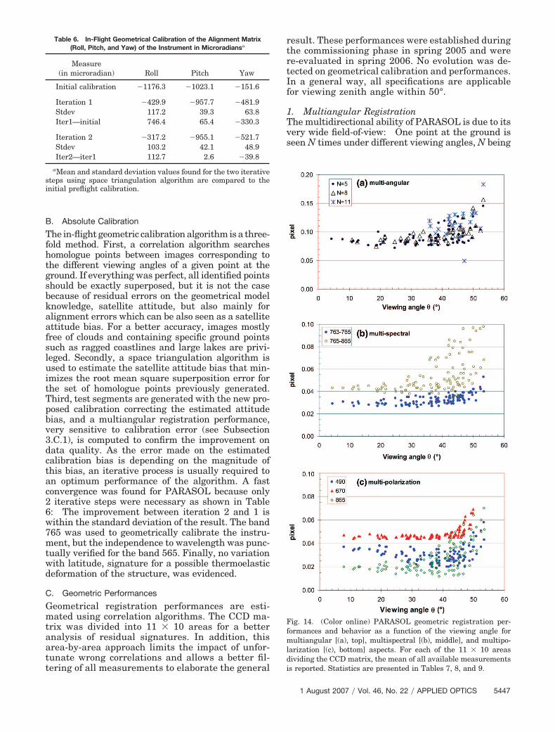
Fig. 14. (Color online) PARASOL geometric registration per-formances and behavior as a function of the viewing angle formultiangular [(a), top], multispectral [(b), middle], and multipo-larization [(c), bottom] aspects. For each of the 11 10 areasdividing the CCD matrix, the mean of all available measurementsis reported. Statistics are presented in Tables 7, 8, and 9.
Table 6. In-Flight Geometrical Calibration of the Alignment Matrix(Roll, Pitch, and Yaw) of the Instrument in Microradiansa
aMean and standard deviation values found for the two iterativesteps using space triangulation algorithm are compared to theinitial preflight calibration.
up to 16. Each viewing angle is separated from theprevious one by approximately 20 seconds and 9° andis derivate from a different raw image [1]. On thelevel-1 data processing chain [5], the N acquisitionsare registered for each level-1 pixel with a given ac-curacy strongly dependent on residual biases on thegeometric correction, i.e., on the calibration error.The multiangular registration performance is as-sessed by a correlation algorithm using images ac-quired for the band 765 and separated by N viewingdirections, N varying from 1 to 16. Table 9 reportsregistration performances for 7 values of N. Themean performances per area �11 10 areas) areillustrated in Fig. 14(a) where it is evidenced that theregistration evaluation is increasing for large viewingangles: in fact, this evaluation is the real perfor-mance plus a correlation error that includes a sensi-ble bidirectional effect of targets. Consequently, thereal performance is within the estimation, and thespecification is considered as met. The performanceestablished during the commissioning phase in March2005 has been verified after one year in orbit (Table 9)and the absence of temporal evolution proves that theinstrumental alignment, i.e., the geometric calibra-tion, is perfectly stable with time.
2. Multispectral RegistrationThe 9 spectral bands presented in Table 2 are notacquired simultaneously, but successively during oneturn of the filter wheel in 20.096 seconds. The spec-tral information is registered on the geometric level-1
processing using the geometric model of the instru-ment (see Subsection 3.A) [5]. The multispectral reg-istration performance is assessed by a correlationalgorithm using images acquired for a couple of spec-tral bands. The estimated performance includes thereal performance plus a correlation error dependingon the observed target and on the considered wave-length. Figure 14(b) and Table 8, the estimationmade for the couple of bands 763–765 is better thanother couples by nearly a factor of 2. This is explainedby the fact that these 2 spectral bands observed avery similar spectral scene, only differing by an at-tenuation due to the dioxygen absorption. Figure14(b) shows the 763–765 performances are consid-ered as the more realistic evaluation for the realmultispectral performance and are clearly underspecification. The performance established duringthe commissioning phase has been verified after oneyear in orbit (Table 8), and the absence of temporalevolution proves that the instrumental geometricmodel is perfectly stable with time.
3. Multipolarization RegistrationFor a polarized triplet, 3 acquisitions are realized fora polarizer oriented at �60° �X-60�, 0° (X0), and �60°(X60) from a given reference [1]. These 3 componentsare successively acquired in 1 second during whenthe observed ground target moves in the field-of-viewdue to the satellite progression, mainly along track,and the Earth rotation, mainly cross track. Onboardregistration of the 3 components is ensured by prisms
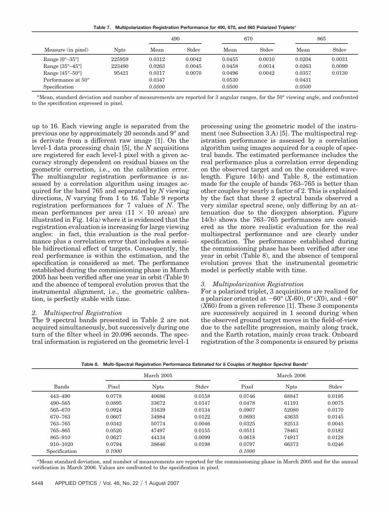
Table 7. Multipolarization Registration Performance for 490, 670, and 865 Polarized Tripletsa
aMean, standard deviation and number of measurements are reported for 3 angular ranges, for the 50° viewing angle, and confrontedto the specification expressed in pixel.
Table 8. Multi-Spectral Registration Performance Estimated for 8 Couples of Neighbor Spectral Bandsa
aMean standard deviation, and number of measurements are reported for the commissioning phase in March 2005 and for the annualverification in March 2006. Values are confronted to the specification in pixel.
viewing forward (for X-60) and backward (for X60)compensating the satellite progression, about 6 kmper second, while the Earth rotation is compensatedat first order by a yaw-steering of the satellite plat-form. The multipolarization registration performanceof the polarized triplet, defined as the radius of thecircle at the Earth surface containing the 3 compo-nents X-60, X0, and X60, is assessed by a correlationalgorithm. Results are presented in Table 7 and il-lustrated in Fig. 14(c) as a function of the viewingangle. The performance for the band 670 is close to0.05 and equivalent whatever the viewing angle (ex-cept for large angles near 50°), while the band 490 ismore optimized on the 35–45° range and the band865 more optimized for near-nadir viewing angle inthe range 0–35°. Performances estimated during thecommissioning phase were reevaluated after one yearin orbit, and no temporal evolution has been detected.
4. Absolute Location AccuracyThe absolute location of level-1 data product was es-timated using ground control manual pointing andusing as reference VEGETATION�SPOT5 products forwhich the absolute location accuracy is within 150 mcompared to the 6 km of the PARASOL resolution[34]. A few VEGETATION products were ordered atthe CTIV with the same specific reprojection thanPARASOL products (equal area sinusoidal projec-tion). Images were selected over France, Australia,Arabia, and Canada in mid 2005. Table 10 shows
statistics for nearly one hundred points of measure-ments and a very good performance close to 2 km.Specification is met and goal performance is nearlysatisfied.
4. Conclusion
In-flight characterization and validation of preflightestimations were presented for both radiometric andgeometric aspects. PARASOL in-flight performanceswere evaluated during the commissioning phase inspring 2005 regarding to the mission specifications,and concluding to adequate level-1 product qualityfor scientific exploitation. The only identified limita-tion was a very poor quality of the band 443 due to anunresolved stray-light problems, and it is stronglyrecommended not to use measurements from thisspectral band. After one year in orbit, performanceswere re-evaluated: All radiometric and geometricperformances were confirmed, even if a light radio-metric temporal decrease was detected, modeled, andcorrected conducting to a rereprocessing of the entirelevel-1 data archive ended in November 2006 [35].The new Version 3 PARASOL level-1 archive is avail-able at CPP (Centre de Production POLDER) at http://polder.cnes.fr/.
Appendix A: Acronyms
ADEOS Advanced Earth Observing Satel-lite
CALIPSO Cloud-Aerosol Lidar and InfraredPathfinder Satellite Observations
CCC Centre de Commande ContrôleCCD Charge coupled deviceCERES Clouds and Earth’s radiant energy
systemCLOUDSAT CLOUD SatelliteCNES Centre National d’Etudes SpatialesCPP Centre de Production POLDERCTIV Centre de Traitement des Images
VEGETATION
ENVISAT Environmental SatelliteLIT Long integration timeMERIS Medium Resolution Imaging Spec-
trometer
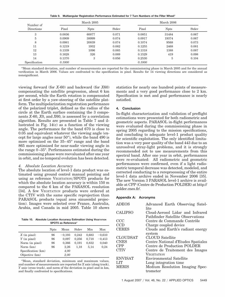
Table 9. Multiangular Registration Performance Estimated for 7 Turn Numbers of the Filter Wheela
aMean standard deviation, and number of measurements are reported for the commissioning phase in March 2005 and for the annualverification in March 2006. Values are confronted to the specification in pixel. Results for 14 viewing directions are considered asnonsignificant.
Table 10. Absolute Location Accuracy Estimation Using VEGETATION
SPOT5 as Referencea
Npts Mean Stdev Min Max
X (in pixel) 96 �0,193 0,242 0,683 �0,610Y (in pixel) 96 0,097 0,256 0,718 �0,413Norm (in pixel) 96 0,366 0,191 0,832 0,040Norm (km) 96 2,26 1,18 5,14 0,24Specification (km) 4,00Objective (km) 2,00
aMean, standard deviation, minimum and maximum values,and number of measurements are reported for X axis (along track),Y axis (cross track), and norm of the deviation in pixel and in km,and finally confronted to specifications.
NIR Near-infraredPARASOL Polarization & Anisotropy of Re-
flectance for Atmospheric Sciencescoupled with Observations from aLidar
POLDER Polarization and Directionality ofEarth Reflectances
SeaWiFS Sea-Viewing Wide Field-of-viewSensor
SIT Short integration timeSQI Système Qualité Image PARASOLSPOT Satellite Pour l’Observation de la
TerreSRI Spectral response of the InstrumentTOA Top of atmosphere
We are very grateful to all those who have contrib-uted to the elaboration of this large collection of con-cluding results mainly at the PARASOL project,CNES�CCC (Centre de Commande Contrôle), CNES�CPP (Centre de Production POLDER) and CNES�SQI(Système Qualité Image PARASOL): M. Bach, P.Lier, F. Serene, P. Henry, C. Dabin, R. Reich, F. Bailly-Poirot, E. Orsal, E. Tolsan, E. Espié, F. Meunier, J.Rollin, R. Bach, S. Leguevaques, D. Toustou, and sci-entists from Laboratoire d’Optique Atmosphérique(LOA, Lille, France) and Laboratoire des Sciences duClimat et de I’Environnement (LSCE, Saclay, France)for their helpful discussions.
References1. P. Y. Deschamps, F.-M. Bréon, M. Leroy, A. Podaire, A. Bricaud,
J.-C. Buriez, and G. Sèze, “The POLDER mission: instrumentcharacteristics and scientific objectives,” IEEE Trans. Geosci.Remote Sens. 32, 3598–3615 (1994).
2. M. Thoby, “Myriad: CNES Micro-Satellite Program,” pre-sented at the 15th Annual AIAA�USU Conference on SmallSatellites, Logan, Utah, 13–16 August 2001, paper SCO1-I-8.
3. B. Fougnie, G. Bracco, B. Lafrance, C. Ruffel, O. Hagolle, andC. Tinel, “In-flight performances of PARASOL inside the aqua-train atmospheric observatory,” presented at the AGU FallMeeting, San Francisco, California, 5–9 December 2005, paperA33C-915.
4. O. Hagolle, P. Goloub, P.-Y. Deschamps, H. Cosnefroy, X. Bri-ottet, T. Bailleul, J. M. Nicolas, F. Parol, B. Lafrance, and M.Herman, “Results of POLDER in-flight calibration,” IEEETrans. Geosci. Remote Sens. 37, 1550–1566 (1999).
5. O. Hagolle, A. Guerry, L. Cunin, B. Millet, J. Perbos, J. M.Laherrère, T. Bret-Dibat, and L. Poutier, “POLDER level 1 pro-cessing algorithms,” in Algorithms for Multispectral and Hyper-spectral Imagery II, Proc. SPIE 2758, pp. 308–319 (1996).
6. T. Bret-Dibat, Y. Andre, and J. M. Laherrère, “Preflight cali-bration of the POLDER instrument,” Remote Sensing and Re-construction for three Dimensional Objects and Scenes, Proc.SPIE 2572, doi:10.1117/12.221357 (1995).
7. B. Lafrance, C. Ruffel, and B. Fougnie, “PARASOL pre-flightradiometric calibration—synthesis report,” CNES Tech. Memo.PAR-NT-S7-6423-CNS (Centre National d’Etudes Spatiales,Toulouse, France, 2005).
8. B. Fougnie, P. Henry, F. Cabot, A. Meygret, and M.-C. Laubies,“VEGETATION: in-flight multi-angular calibration,” in Earth Ob-serving Systems V, Proc. SPIE 4135, 331–338 (2000).
9. B. Fougnie, O. Hagolle, and F. Cabot, “In-flight measurementand correction of non-linearity of the POLDER-1’s sensitivity,”presented at the 8th Symposium of the International Societyfor Photogrammetry and Remote Sensing, Aussois, France,8–12 January 2001.
10. J. M. Laherrère, L. Poutier, T. Bret-Dibat, O. Hagolle, C.Baqué, P. Moyer, and E. Verges, “POLDER on-ground straylight analysis, calibration and correction,” presented at Eu-ropto Conference on Sensors, Systems and Next GenerationSatellites III, London, UK, 22–26 September 1997.
11. R. E. Eplee, Sean W. Bailey D. Wayne D. Robinson D. K. Clark,P. J. Werdell, M. Wang, R. A. Barnes, and C. R. McClain,“Calibration of SeaWiFS. II. Vicarious Techniques,” Appl. Opt.40, 6701–6718 (2001).
12. O. Hagolle and F. Cabot, “Calibration of MERIS using naturaltargets,” presented at the Second MERIS and AATSR Cali-bration and Geophysical Validation Workshop, Frascati, Italy,20–24 March 2006.
13. B. Fougnie, P. Y. Deschamps, and R. Frouin, “Vicarious Cali-bration of the POLDER ocean color spectral bands usingin-situ measurements,” IEEE Trans. Geosci. Remote Sens. 37,1567–1574 (1999).
14. B. Fougnie, B. P. Henry, A. Morel, D. Antoine, and F. Mon-tagner, “Identification and characterization of stable homoge-neous oceanic zones: climatology and impact on in-flightcalibration of space sensor over Rayleigh scattering,” pre-sented at Ocean Optics XVI, Santa Fe, New Mexico, 18–22November 2002.
15. E. Shettle and R. Fenn, “Models for the aerosols of the loweratmosphere and the effects of humidity variations on theiroptical properties,” AGFL-TR-79-0214, U.S. Air Force Geo-phys. Lab. (Hanscom Air Force Base, 1979), p. 94.
16. E. Vermote, R. Santer, P.-Y. Deschamps, and M. Herman,“In-flight calibration of large field of view sensors at shorterwavelengths using Rayleigh scattering,” Int. J. Remote Sens.13, 3409–3429 (1992).
17. C. Cox and W. Munk, “Measurements of the roughness of thesea surface from photographs of the sun’s glitter,” J. Opt. Soc.Am. 44, 838–850 (1954).
18. O. Hagolle, J. M. Nicolas, B. Fougnie, F. Cabot, and P. Henry,“Absolute calibration of VEGETATION derived from an interbandmethod based on sunglint over ocean sites,” IEEE Trans.Geosci. Remote Sens. 42, 1–10 (2004).
19. B. Toubbé, T. Bailleul, J. L. Deuzé, P. Goloub, O. Hagolle, andM. Herman, “In-flight calibration of the POLDER polarizedchannels using the sun’s glitter,” IEEE Trans. Geosci. RemoteSens. 37, 513–525 (1999).
20. C. Vanbauce, J. C. Buriez, F. Parol, B. Bonnel, G. Sèze, and P.Couvert, “Apparent pressure derived from ADEOS-POLDERobservations in the oxygen A-band over ocean,” Geophys. Res.Lett. 25, 3159–3162 (1998).
21. B. Lafrance, O. Hagolle, B. Bonnel, Y. Fouquart, and G.Brogniez, “Interband calibration over clouds for POLDER spacesensor,” IEEE Trans. Geosci. Remote Sens. 40, 131–142 (2002).
22. H. Cosnefroy, M. Leroy, and X. Briottet, “Selection and char-acterization of Saharian and Arabian desert sites for the cal-ibration of optical satellite sensors,” Remote Sens. Environ. 58,101–114 (1996).
23. F. Cabot, O. Hagolle, C. Ruffel, and P. Henry, “Remote sensingdata repository for in-flight calibration of optical sensors overterrestrial targets,” in Earth Observing Systems IV, Proc. SPIE3750, 514–523 (1999).
24. B. Fougnie, F. Cabot, O. Hagolle, and P. Henry, “CNES con-
tribution to ocean color calibration: cross-calibration overdesert sites,” SIMBIOS Project 2001 Annual Report, NASA�TM-2002-210005 (NASA, 2002), pp. 159–163.
25. H. Rahman and G. Dedieu, “SMAC: a simplified method for theatmospheric correction of satellite measurements in the solarspectrum,” Int. J. Remote Sens. 15, 123–143 (1994).
26. R. A. Barnes and F. Zalewski, “Reflectance-based calibration ofSeaWiFS: I. Calibration coefficients,” Appl. Opt. 42, 1629–1647 (2003).
27. L. Bourg and S. Delwart, “MERIS instrument calibration,”presented at the Second MERIS and AATSR Calibration andGeophysical Validation Workshop, Frascati, Italy, 20–24March 2006.
28. X. Xiong and W. Barnes, “An overview of MODIS radiometriccalibration and characterization,” Adv. Atmos. Sci. 23, 69–79(2006).
29. R. A. Barnes, R. E. Eplee, G. M. Schmidt, F. S. Platt, and C. R.McClain, “Calibration of SeaWiFS. I. Direct techniques,” Appl.Opt. 40, 6682–6700 (2001).
30. D. Six, M. Fily, S. Alvain, P. Henry, and J. P. Benoist, “Surface
characterization of the Dome Concordia area (Antarctica) as apotential satellite calibration site, using SPOT-4 VEGETATION
instrument,” Remote Sens. Environ. 89, 83–94 (2004).31. IOCCG, “In-flight calibration of ocean Color Sensor,” Reports of
the International Ocean-Color Coordinating Group, R. Frouin,ed. (Dartmouth, Canada, to be published).
32. J. C. Buriez, C. Vanbauce, F. Parol, P. Goloub, M. Herman, B.Bonnel, Y. Fouquart, P. Couvert, and G. Sèze, “Cloud detectionand derivation of cloud properties from POLDER,” Int. J. Re-mote Sens. 18, 2785–2813 (1997).
33. N. A. J. Schutgens, L. G. Tilstra, P. Stamnes, and F. M. Bréon,“On the relationship between Stokes parameters Q and Uof atmospheric ultraviolet�visible�near-infrared radiation,”J. Geophys. Res. 109, D09205, doi:10.1029/2003JD004081(2004).
34. S. Sylvander, I. Albert-Grousset, and P. Henry, “Geometricperformances of the VEGETATION products,” IEEE Interna-tional Geosciences And Remote Sensing Symposium (IEEE,2003), Vol. 1, pp. 573–575.


![Parasol Houses [Louis Kahn]](https://static.documents.pub/doc/80x56/55cf9bf8550346d033a80c29/parasol-houses-louis-kahn.jpg)


