William E. Griffiths and Gholamreza Hajargasht

Department of Economics

Working Paper Series

June 2012

Research Paper Number 1149

ISSN: 0819 2642

ISBN: 978 0 7340 4499 0

Department of Economics The University of Melbourne Parkville VIC 3010 www.economics.unimelb.edu.au

Pareto-Lognormal Income Distributions:

Inequality and Poverty Measures, Estimation and Performance

Pareto-Lognormal Income Distributions:

Inequality and Poverty Measures, Estimation and Performance

Gholamreza Hajargasht and William E. Griffiths

Department of Economics

University of Melbourne, Australia

June 26, 2012

ABSTRACT

The (double) Pareto-lognormal is an emerging parametric distribution for income that

has a sound underlying generating process, good theoretical properties, and favourable

evidence of its fit to data. We extend existing results for this distribution in 3 directions.

We derive closed form formula for its moment distribution functions, and for various

inequality and poverty measures. We show how it can be estimated from grouped data

using the GMM method developed in Hajargasht et al. (2012). Using grouped data from

ten countries, we compare its performance with that of another leading 4-parameter

income distribution, the generalized beta-2 distribution. The results confirm that both

distributions provide a good fit, with the double Pareto-lognormal distribution

outperforming the beta distribution in some but not all cases.

Keywords: GB2 distribution, GMM, moment distributions, double-Pareto.

JEL Classification: C13, C16, D31

2  

I. Introduction

For more than a century considerable effort has been directed towards providing new

functional forms for income distributions. A major motivation of such studies has been to

suggest functions with theoretical properties and statistical fits that are better than those of

functions already appearing in the literature. The large number of functional forms that has

been suggested includes, but is not limited to, the lognormal, gamma, Pareto, Weibull,

Dagum, Singh-Maddala, beta-2, and generalized beta-2 distributions, and the quest

continues. See Kleiber and Kotz (2003) for a comprehensive review. An emerging 4-

parameter distribution for income and other phenomena is the double Pareto-lognormal

distribution (hereafter dPLN) developed by Reed (2003) and studied further by Reed and

Jorgensen (2004)1. It has good properties with a sound theoretical justification (Reed 2003),

and, according to Reed and Wu (2008), provides a very good fit to income data.

The purpose of this paper is to provide some further results for this distribution. We

derive closed form solutions for various inequality and poverty measures in terms of the

parameters of the dPLN distribution and show how they relate to the corresponding

inequality and poverty measures for the lognormal and Pareto distributions. We also provide

the moment distribution functions which are required for estimating the dPLN distribution

from grouped data within the GMM framework developed in Hajargasht el. (2012). Results

from estimating this model are compared with those from estimating another leading 4-

parameter distribution known as the generalized beta of the second kind (hereafter GB2),

developed by McDonald (1984) and McDonald and Xu (1995)2. Using grouped data from

ten regions (China rural, China urban, India rural, India urban, Pakistan, Russia, Poland,

Brazil, Nigeria and Iran), we estimate the GB2, a 3-parameter Pareto-lognormal, and the

dPLN distributions, and compare their performance in terms of goodness of fit. The results

                                                            1 - According to “GoogleScholar”, these papers have 107 and 114 citations, respectively. 2 ‐ According to “GoogleScholar”, these papers have 420 and 215 citations, respectively. 

3  

suggest that all three distributions provide good fits, and there is not one particular

distribution that dominates the others over all data sets.

The paper is organized as follows. In Section II we briefly review the dPLN

distribution. Expressions are provided for its moment distribution functions needed for

GMM estimation and for various inequality and poverty measures. The GB2 distribution that

we later compare with the dPLN is reviewed in Section III. In Section IV we summarize the

GMM methodology developed in Hajargasht et al. (2012) for estimating the parameters of a

general income distribution, and show how it can be applied to the dPLN distribution.

Section V contains a description of the data used to illustrate the theoretical framework, and

the results. The results include parameter estimates and their standard errors, test results for

excess moment conditions, mean-square-error comparisons for goodness-of-fit, and Gini and

Theil coefficients. Concluding remarks are provided in Section VI.

II. Pareto-lognormal income distributions

The probability density function (pdf) of the dPLN distribution with parameters ( , , , )m is

1 2

ln( ; , , , )

( )dPLN y m

f y m R x R xy

(1)

where ( ) 1 ( ) ( )R t t t is a Mill’s ratio, (.) and (.) are, respectively, the pdf and

cumulative distribution function (cdf) for a standard normal random variable,

1 2

ln lnand

y m y mx x

The cdf of the dPLN distribution has been derived as (Reed and Jorgensen 2004)

1 2

0

ln ln ( ) ( )( ; , , , ) ( )

ydPLN y m y m R x R x

F y m f t dt

(2)

Two attractive features of the dPLN distribution are that it can be derived from

reasonable assumptions about the generation of incomes, and that it accords with empirical

4  

observation. It is derived by relaxing some of the assumptions of earlier models of income

generation. Gibrat (1931) showed that if the income of each individual at time t grows

randomly but proportionately with respect to their income in the previous time, the emerging

distribution is lognormal. Variations on this theme were shown to generate features of the

Pareto distribution (Champernowne 1953, Mandelbrot 1960). Reed (2001, 2003) and Reed and

Jorgensen (2004) developed and extended these earlier models, using the assumption that

income generation follows a geometric Brownian motion (GBM) process, the continuous time

version of assumptions made by Gibrat and Champernowne. Within this framework, if income

growth is modeled by GBM with a fixed initial state, then after a fixed time T, incomes follow a

lognormal distribution. If we relax the assumption that T is fixed, recognizing that income

earning ceases at different times for different individuals, assume that T follows an exponential

distribution, and assume that the all income earners start with the same income, normalized to

unity, then the resulting income distribution is a double-Pareto distribution with pdf

1

1

for 0 1( )

( ; , )

for 1( )

dP

y y

f y

y y

, 0 (3)

This pdf exhibits Pareto behaviour in both tails. It is proportional to y raised to a negative power

in the right tail; in the left tail it is proportional to y raised to a positive or negative power

depending on whether or not 1 . It has also been derived by Benhabib and Zhu (2008) as an

emerging distribution for wealth in an elaborate overlapping generation model with utility

maximizing agents.

The dPLN distribution in (1) is a generalization of the double-Pareto distribution

obtained by relaxing the assumption that all income earners have the same initial income, and

assuming instead that starting incomes are lognormally distributed, and then evolve according

to GBM. It can be derived as the distribution of the product of a double-Pareto random variable

5  

with parameters ( , ) and a lognormal random variable with parameters ( , )m . It has Pareto

behaviour in both the upper and lower tails. That is,

1 11 2( ) ( ) and ( ) ( 0)f y c y y f y c y y

where 1c and 2c are constants. Apart from the tail behavior, it is shaped somewhat like a

lognormal distribution, providing 1 ; it is monotonically decreasing for 0 1 . The

desirability of Pareto behavior in the upper tail has been well documented; there have been

claims that similar behavior can be observed in the left tail (Champernowne 1953). If

( , ) , the dPLN tends to a lognormal distribution and for large values of ( , ) , it is

close to lognormal. If we have only , we obtain the 3-parameter Pareto-lognormal (PLN)

distribution that shows Pareto behavior only in the upper tail. This distribution has studied by

Colombi (1990). We include it as one of the distributions we estimate in our empirical work. Its

pdf and cdf are given respectively by

1

ln( ; , , )PLN y m

f y m R xy

(4)

1

ln ln( ; , , ) ( )PLN y m y m

F y m R x

(5)

For estimating the dPLN and PLN distributions using the GMM method of Hajargasht

et al. (2012), and for finding closed form formulas for some poverty measures, we need the

dPLN and PLN moments and moment distribution functions of orders one and two. From Reed

and Jorgensen (2004), the k-th moments (which exist for k ) are given by

2 2

exp( )( ) 2

dPLNk

kkm

k k

(6)

2 2

exp2

PLNk

kkm

k

(7)

We show in Appendix A that the moment distribution functions are given by

6  

0

1 2

1( ; , , , ) ( )

ln ln ( ) ( ) ( ) ( )

ydPLN k dPLN

k dPLNk

F y m t f t dt

y m y m k R x k R xk k

(8)

0

1

1( ; , , ) ( )

ln ln( )

yPLN k PLN

k PLNk

F y m t f t dt

y m y mk k R x

(9)

Because income distributions are often used to assess inequality and poverty, it is

desirable to express inequality and poverty measures in terms of the parameters of those

distributions. Such expressions show explicitly the dependence of inequality or poverty on each

of the parameters, and they facilitate calculation of standard errors for inequality or poverty

indices. In Appendix B we derive expressions for the Gini, generalized entropy, Theil, and

Atkinson inequality measures in terms of the parameters of the dPLN and PLN distributions.

Details of these measures can be found in a variety of sources. See, for example, Cowell (2007),

and Kleiber and Kotz (2003). Here we report the results for the Gini and Theil measures; results

for the others are given in Appendix B.

The most widely used inequality measure is the Gini coefficient. For the dPLN

distribution, it is given by

2

2

(1 )exp ( 1) (1 2 )1 2

( )(2 1)(1 )2 2

( 1)exp ( 1) ( 1 2 )

( )(1 2 )(1 ) 2

dPLNG

(10)

and for the PLN model it simplifies to

22exp ( 1) (1 2 )

2 1(2 1) 2 2

PLNG

(11)

7  

The Gini coefficient for lognormal distribution with parameter is 2 2 1 , that for a

left tail Pareto is 1(1 2 ) , and that for a right tail Pareto is 1(2 1) . Thus, dPLNG and PLNG

are both equal to the Gini coefficient for a lognormal distribution plus weighted adjustment(s)

for the Pareto tails.

A second commonly used inequality measure is the Theil index defined as

0

ln ( )y y

T f y dy

In Appendix B we show that, for the dPLN distribution,

21 1 1 1

ln ln( 1) ( 1) 2

dPLNT

(12)

and for the PLN distribution it becomes

21 1

ln1 2

PLNT

(13)

In this case we have the interesting result that the Theil measure is equal to the sum of the Theil

measure for a lognormal distribution 2 2 and the relevant measure(s) for the Pareto

distributions, 1ln ( 1) 1

and 1ln ( 1) 1

.

We provide details for five poverty measures the headcount ratio, poverty gap, Foster-

Greer-Thorbecke (2FGT , Atkinson and Watts measures. With the exception of the Watts

measure, all these quantities can be written in terms of the moments and moment distribution

functions provided in equations (2) and (5)-(9). Thus, for computing in these cases, it is

sufficient to give general expressions that hold for all distributions and to rely on the earlier

moment and moment-distribution equations for the dPLN and PLN distributions. The Watts

measure requires more work. Derivation of expressions for this measure for the dPLN and PLN

8  

distributions are given in Appendix C. General details of the various measures and many others

are conveniently summarized in Kakwani (1999).

The head-count ratio is given by the percentage of population below a target level of

income Py , called the poverty line. That is, ( )PF y . The poverty gap is a modification that takes

into account how far the poor are below the poverty line. It is given by

1

0

( ) ( ) ( )Py

PP P

P P

y yPG f y dy F y F y

y y

(14)

The measure (2FGT is similar, but weights the gap between income and the poverty line

more heavily. It is given by

2

21 22

0

2(2 ( ) ( ) ( ) ( )

Py

PP P P

P P P

y yFGT f y dy F y F y F y

y y y

(15)

Another generalization of the poverty gap is the Atkinson index given by

0

1 1( ) 1 ( ) ( ) ( )

Pye

eP e Pe

P P

yA e f y dy F y F y

e y e y

(16)

where e is a parameter for the degree of inequality aversion.

The Watts index, shown by Zheng (1993) to satisfy all axiomatic conditions, is given by

0

ln ( )Py

PW y y f y dy

In Appendix C we show that, for the dPLN distribution,

( ) ( ) ln ln( ) ( )

( ) ( )dPLN PLN PLN P P

P P P

y m y mW F y F y y

(17)

For the DPL distribution it becomes

( )1 ln ln( )PLN PLN P P

P P

y m y mW F y y

(18)

9  

where ( ) ( )PLNF y is the cdf of the PLN distribution with Pareto behaviour in the right tail,

( ) ( )PLNF y is cdf of the PLN distribution with Pareto behaviour in the left tail, and the last term

in both equations is the Watts index for a lognormal distribution. See Muller (2001).

Once the parameters of the distributions have been estimated, these expressions are

convenient ones for computing the various poverty measures.

III. The generalized beta distribution of the second kind

For a distribution with which to compare the performance of the PLN and dPLN distributions,

we chose the GB2 distribution whose pdf with positive parameters ( , , , )a b p q is

1

( ; , , , )

, 1

ap

p qaap

ayf y a b p q

yb B p q

b

0y (19)

where ( , )B is the beta function. Like the dPLN, the GB2 income distribution is derived from a

reasonable economic model. Parker (1999) shows how it arises from a neoclassical model with

optimizing firm behaviour under uncertainty where the shape parameters p and q become

functions of the output-labor elasticity and the elasticity of income returns with respect to

human capital. Another very useful feature of the GB2 is that it nests many popular income

distributions as special or limiting cases, including the beta-2, Singh-Maddala, Dagum,

generalized gamma and lognormal distributions. Its detailed properties are given by McDonald

(1984), McDonald and Xu (1995), and Kleiber and Kotz (2003), with further information on

inequality measures provided by McDonald and Ransom (2008) and Jenkins (2009). Hajargasht

et al. (2012) show how to find GMM estimates of its parameters from grouped data. The

quantities needed for GMM estimation, and also for computing poverty measures, are the

moments and moment distribution functions given respectively by

2 ,

,

kGBk

b B p k a q k a

B p q

(20)

10  

2 2( ; , , , ) ; , , , ,GB GBk u

k k k kF y a b p q F y a b p q B p q

a a a a

(21)

where 1a a

u y b y b and 1 1

0( , ) (1 ) ( , )

u p quB p q t t dt B p q is the cdf for a

standard beta random variable defined on the (0,1) interval. Note that the cdf for the GB2 is

given by 2 20( ; , , , ) ; , , ,GB GBF y a b p q F y a b p q . Also, the moments of order k exist only if

ap k aq .

IV. The GMM estimator

To describe the general form of the GMM estimator for estimating an income distribution from

grouped data, we begin with a sample of T observations 1 2, , , Ty y y , assumed to be

randomly drawn from an income distribution ( ; )f y , where is a vector of unknown

parameters, and grouped into N income classes 0 1( , ),z z 1 2( , ),z z …, 1( , )N Nz z , with 0 0z and

Nz . The available data are the mean class incomes 1 2, , , Ny y y and the proportions of

observations in each class 1 2, , , Nc c c . The estimation problem is to estimate , along with

unknown class limits 1 2 1, , , Nz z z . To tackle this problem, Hajargasht et al. (2012) proposed a

GMM estimator given by

ˆ argmin ' θθ H θ H θ (22)

where 1 2 1, , , ,Nz z z θ ,

1

1,

T

tt

yT

H θ h θ

is a set of moments set up for the ic and iy such that E H θ 0 , and is the weight

matrix

1

1

1plim , ,

T

t tt

y yT

h θ h θ (23)

11  

The first N elements in the (2 1)N vector ,tyh θ are

i t ig y k θ 1,2, ,i N (24)

where i tg y is an indicator function such that

11 if

0 otherwise

i i

i

z y zg y

and

1 0

( ; ) ;i

i

z

i i i

z

k f y dy g y f y dy E g y

θ

The second set of N elements in the (2 1)N vector ,tyh θ are

t i t iy g y θ 1,2, ,i N (25)

where

1 0

( ; ) ;i

i

z

i i i

z

y f y dy yg y f y dy E yg y

θ (26)

With these definitions, we can write

1

1 ;

T

tt

yT

c kH θ h θ

y (27)

where c, k, and are N-dimensional vectors containing the elements ,i ic k and i ,

respectively, and, using 1

( )T

i i ttT g y , the i-th element of y is given by

1 1

1 1( ) ( )

T Ti

i i i t i t t i tt ti

Ty c y y g y y g y

T T T (28)

Hajargasht et al. (2012) show that the weight matrix can be written as

1 3

3 2

( ) ( )

( ) ( )

D D

D D

(29)

12  

where ( )D denotes a diagonal matrix with elements of the vector on the diagonal. The

elements in the vectors 1 , 2 , and 3 are

(2)1i i iv , 2i i ik v , and 3i i iv , where

1

(2) 2 2 2

0

( ; ) ;i

i

z

i i i

z

y f y dy y g y f y dy E y g y

θ (30)

and (2) 2i i i iv k . Collecting all these various terms, the GMM objective function in (22) can

be written as

1 3

3 2

2 21 2 3

1 1 1

( ) ( )

( ) ( )

( ) ( ) 2 ( )( )N N N

i i i i i i i i i i ii i i

GMM

c k y c k y

D Dc k c kH H

D Dy y

(31)

Equations (22) to (31) are a useful summary of the results in Hajargasht et al. (2012),

and equation (31) is a computationally convenient expression for finding the GMM estimator

for . However, the above results mask much of the development that led to the final result in

(31). Because 1 11

N N

i ii ik c θ , one of the moment conditions in H θ (see equation

(27)) is redundant, and, unless we consider a generalized inverse, the inverse defined in (23)

does not exist. Hajargasht et al. set up (2 1)N non-redundant moment conditions, derived the

corresponding matrix 1 , and found its inverse . They then showed that the relatively

complicated objective function, expressed in terms of a (2 1) 1N vector H, and a

(2 1) (2 1)N N matrix , can be written much more simply in terms of the 2N -

dimensional versions of H and given in equation (31). If K is the dimension of (the

number of unknown parameters in the income density), there are a total of ( 1 )N K

unknown parameters. Given there are (2 1)N non-redundant moment conditions, the number

of excess moment conditions is ( )N K .

13  

The quantities ,i ik and (2)i are all functions of the unknown parameters , and will

depend on the assumed form of the income distribution. For most distributions it is convenient

to compute these quantities by expressing them in terms of the distribution function and the first

and second moment distribution functions of the assumed distribution. Specifically,

1( ; ) ( ; )i i ik F z F z θ (32)

1 1 1( ; ) ( ; )i i iF z F z θ (33)

and

(2)2 2 2 1( ) ( ; ( ;i i iF z F z (34)

The right-hand-side quantities in these equations can be obtained from equations (2), (6) and (8)

for the dPLN distribution, (5), (7) and (9) for the PLN distribution and (20) and (21) for the

GB2 distribution.

In our empirical work we employed an iterative two-step GMM estimator. In the first

stage we find 1 0ˆ argmin ' θθ H θ H θ where 2 2 2 2 2 2

0 1 2 1 2( , , , , , , , )N Nc c c y y y D . In the

second stage we find 2 1ˆ ˆarg min ' θθ H θ θ H θ , and then we iterate until convergence.

The rationale behind using 0 in the first step is that it leads to an estimator that minimizes the

sum of squares of the percentage errors in the moment conditions.

The asymptotic covariance for can be shown to be

1

1 3

3 2

( ) ( )1ˆvar( ) ( )T

D D k θk mθ

D D m θθ θ

(35)

This expression can be used to compute standard errors for the elements in and functions of

them. In our empirical work we successfully used numerical derivatives to compute (35).

Under the null hypothesis that the moment conditions are correct E H θ =0 , the J

statistic

14  

2ˆ ˆ ˆ' dN KJ T H θ W θ H θ (36)

where N K is the number of excess moment conditions. In traditional GMM estimation this

test statistic is used to assess whether excess moment conditions are valid. In our case, since we

assume a particular form of parametric income distribution, and use its properties to construct

the moment conditions and weight matrix, the J statistic can be used to test the validity of the

assumed income distribution.

V. Description of data and empirical analysis

To compare GB2, PLN and dPLN distributions, we used grouped data from the ten “regions”

China urban, China rural, India urban, India rural, Pakistan, Russia, Poland, Brazil, Nigeria and

Iran. These countries represent a mix of different regions and different inequality levels. The

data were downloaded from the World Bank web site http://go.worldbank.org/WE8P1I8250.

Population shares ic and the corresponding income shares is were available for 20 groups for

all regions except for China rural (17 groups) and India rural and urban (12 groups). For

consistency, we converted the data from all regions into 12 groups. Also available from the

World Bank website is each region’s mean monthly income y , found from surveys and then

converted using a 2005 purchasing-power-parity exchange rate. To implement the methodology

described in Section 4 we compute i i i iy c y s y for each of the classes, where the class mean

incomes are given by i i iy s y c .

Sample sizes T for each of the surveys from which the grouped data were computed are

not available. For calculating standard errors, we used 20,000T . This is a conservative value

since most of surveys have sample sizes which are larger. If standard errors for other sample

sizes are of interest, they can be obtained from our results by multiplying by the appropriate

scaling factor.

15  

In what follows we first examine the GMM estimates and standard errors for the

parameters and class limits estimated using the PLN, dPLN and GB2 distributions. Second, we

consider the results of J tests for the validity of the excess moment conditions, comparing the

GB2 distribution with the PLN and dPLN distributions. Then, a goodness-of-fit comparison of

these distributions is made on the basis of their ability to predict the observed income shares for

each group. Finally, we present the Gini and Theil coefficient estimates and their standard

errors obtained under the alternative distributional assumptions.

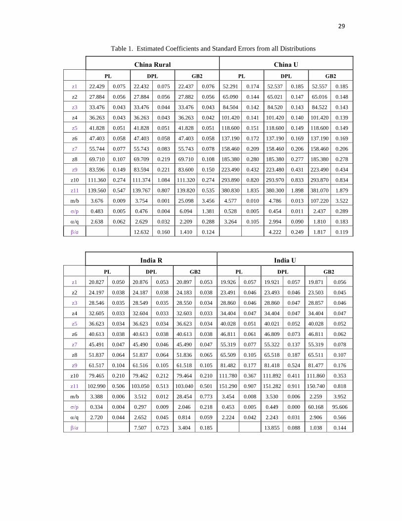
Estimates of the parameters for the three distributions, and the class limits for the

grouped data, are reported in Table 1. We can make the following observations. Estimates of

the class limits are almost identical for each of the models, and their standard errors are small.

Estimates of the parameter for the PLN and dPLN distributions are relatively small, and

significantly different from zero, indicating significant Pareto behaviour in the upper tail of the

distribution. However, estimates for are large in some regions (China rural, India rural and

urban, Pakistan, Poland and Iran), indicating that Pareto behaviour is not significant in the

lower tail. In these instances there was very little difference between corresponding parameters

for the PLN and dPLN models. All standard errors are calculated numerically. They are

relatively small providing reassurance that we are estimating the models accurately, at least for

our assumed sample size. A potential problem that may occur where there is a high level of

inequality and which we encountered when estimating the GB2 and dPLN distributions for

Brazil (but not the PLN distribution), is the non-existence of the second moment. Hajargasht et

al. (2012) found the same problem. For the existence of the k-th moment, the GB2 distribution

requires aq k , and the DPLN and PLN distributions require k . If, in the first step of

estimation using the weighting matrix 0 , the estimates are such that ˆ ˆ 2aq or ˆ 2 , the

optimal weighting matrix in the second step, which requires the existence of second order

moments, cannot be computed. We are unable to proceed with iterative GMM estimation

16  

without modifying the algorithm. In the results reported in Table 1 we overcame the problem

for Brazil by minimizing the objective function subject to the constraint 2aq for the GB2

distribution, and subject to the constraint 2 for the dPLN distribution. This solution may

not be entirely satisfactory. The underlying income distribution may indeed not have second

moments, and the standard errors for the boundary solutions that result may not be valid.

When sample sizes are very large, the probability of rejecting a false null hypothesis can

be close to one, even when the difference between an actual parameter value and the value

hypothesized under the null is so small as to be meaningless. In the context of testing excess

moment conditions to assess the validity for a particular income distribution, this means that a

particular income distribution can be rejected even when it fits the data well, both visually and

in terms of predicting income shares. Given these circumstances, and given that sample sizes

are not available for the regions for which we have data, we use the magnitudes of the J

statistics as a basis for comparing goodness of fit of the three distributions, rather than as a

significance test for the validity of excess moment conditions. Using a sample size of

20,000T , Table 2 provides J-statistic values for all three distributions and for all regions.

The smaller the test value, the better the fit of the distribution. In this sense, the results indicate

better performance of dPLN relative to GB2 for China rural and urban, India rural and Poland,

and better performance of GB2 for the other regions. Also, there are a few regions (China rural

and urban, India urban and Poland) where PLN is marginally better than dPLN. For Brazil all

distributions appear to be a relatively poor fit, with GB2 being the best of the three.

Goodness-of-fit in terms of predicting income shares was also carried out by comparing

the observed income shares is with the predicted income shares derived from the estimated

distributions, defined as 1 1 1ˆ ˆˆ ˆ ˆ; ;i i is F z F z where iz are the estimates of the class limits.

Table 2 contains the percentage root-mean-squared errors, 2

1

1ˆ100

N

i iiN s s

, for all

17  

distributions. The first impressive thing to report about these values is that they are very small.

For example, the RMSE for China rural, using the 3-parameter Pareto-lognormal is

approximately 0.08%. That means that the average error (in the RMSE sense) from predicting

the income shares for this region is 0.0008, a very accurate prediction indeed. One of the worst

performers using this measure is for India rural, using PLN, but even here the average error is

only 0.0083. A comparison of the RMSEs for the three distributions yields similar conclusions

to those reached by examining the J-statistics. The dPLN has better performance relative to

GB2 for 5 regions (China rural and urban, India rural, Poland and Iran) but worse performance

for the other 5 regions. The dPLN has a substantially smaller RMSE than PLN for those regions

where the estimate for was relatively small, and a similar RMSE for those regions where the

estimate for was relatively large.

Estimates of the Gini and Theil inequality measures are given in Table 3. Estimates of

the Gini coefficient are generally comparable across the 3 distributions, with the largest

discrepancy being 0.014 for India urban. A similar remark can be made for the Theil

coefficient, but in this case there are discrepancies for both India urban and Brazil, and the

discrepancies are larger. In the case of India urban, the GB2 leads to a smaller estimate of the

degree of inequality. The restricted parameter estimates for Brazil’s GB2 and dPLN

distributions led to a higher degree of inequality than that estimated from PLN. The regions

with the greatest inequality are Brazil, Nigeria and India urban. For Iran, the Gini coefficient is

comparable to that of India urban, but the Theil coefficient suggests a lower degree of

inequality.

18  

VI. Concluding remarks

The Pareto-lognormal and double Pareto-lognormal distributions have been advocated as good

choices for modelling income distributions because of their sound theoretical base and their

superior empirical goodness-of-fit. We have added to the existing literature in four ways: (1)

Expressions for inequality measures in terms of the parameters of the distributions have been

derived. (2) We show how the distributions can be estimated from grouped data using the

generalized method of moments, and we derive the moment distribution functions required for

GMM estimation. (3) We indicate how the moments and moment distribution functions can be

used to compute a number of poverty measures. An alternative expression is derived for the

Watts poverty index that cannot be expressed in terms of moment distribution functions. (4) For

ten example countries, the performance of the PLN and dPLN distributions is compared with

another popular income distribution, the generalized beta distribution of the second kind. We

find that all three distributions fit the data relatively well, but there is no clear evidence to

suggest that the PLN or the dPLN is superior to the GB2 distribution.

Appendix A Moment Distribution Functions

First consider the following Pareto-lognormal density function

1

1 (ln )ln( )

(ln )PLN y my m

f yy y m

which can be written equivalently as

2 2

1

(ln ) ln( ) exp 1

2PLN y m y m

f yy

To obtain the moment distribution function of order k we must compute

2 21

1

00

(ln ) ln( ) exp 1

2

yy

k PLN k t m t mt f t dt t dt

19  

Let lnu t m so that expt m u and expdt m u du . Then,

(ln )

2 2

1

0

( ) exp exp ( ) 12

y my

k PLNt f t dt km k u u du

Integration by parts leads to

2 2

1

0

(ln )

( ) exp2

lnexp ( )(ln ) 1 exp ( )

yk PLN

y m

t f t dt kmk

y mk y m k u u du

Now,

(ln )2 2 2(ln )

2

2 2 2

1 1exp ( ) exp exp

2 22

lnexp

2

y my m k

k u u du u k du

k y mk

Using this result, we obtain, after some algebra,

2 2

1

0

2 2 2 2

2 2

1

( ) exp2

ln ln ln ln1 exp

2 2

ln lnexp ( )

2

yk PLN k

t f t dt kmk

y m y m y m y m kk k

k y m y mkm k k R x

k

From this result we obtain equation (9), which gives the k-th moment distribution function for

the PLN, with Pareto behavior in the right tail.

To obtain the k-th moment distribution function for the dPLN distribution it is

convenient to first consider the PLN distribution with Pareto behavior in the left tail. Its pdf is

2

1 (ln )ln( )

(ln )PLN y my

f yy y m

20  

Then, using similar steps to those used to derive 1

0

( )y

k PLNt f t dt , we can show that

2 2

2 2

0

ln ln( ) exp ( )

2

yk PLN k y m y m

t f t dt km k k R xk

From Reed and Jorgensen (2004), the density of the dPLN can be expressed as the mixture

1 2( ) ( ) ( )dPLN PLN PLNf y f y f y

Thus,

1 2

0 0 0

2 2

1 2

( ) ( ) ( )

exp( )( ) 2

ln ln ( ) ( ) ( ) ( )

y y yk dPLN k PLN k PLNt f t dt t f t dt t f t dt

kkm

k k

y m y m k R x k R xk k

From this result, we obtain k-th moment distribution function ( ; , , , )dPLNkF y m given in (8).

Appendix B Inequality Measures

1. The Gini Coefficient

To derive the Gini coefficient for the dPLN distribution we use the formula

0

2 ( ) ( )

1

yF y f y dy

G

where the mean is given by

2

exp( 1)( 1) 2

m

The required integral can be written in terms of six components. That is,

1 2 3 4 5 6

0

( ) ( )I yF y f y dy I I I I I I

21  

where the six components arise from the product of two components in the pdf ( )dPLNf y and

three components in the cdf ( )dPLNF y . See equations (1) and (2). Each of the six components

and their solutions follow. We use the transformation lnu y m , integration by parts,

and the following result from Gupta and Pillai (1965),

2

2

exp 2

2 1

x bax b dx

a

2 2

1

2 2 2 2

exp exp (1 ) ( )2

( 1) (1 2 )exp exp

( )( 1) 2 22 2

I u u u du

2 2

2

2 2 2

exp exp (1 ) ( )2

2( ( 1) ) ( 1 2 )exp exp

( )( 1) 2 22 2

I u u u du

222 2

3 2

2 2 22

2

exp exp (1 2 )

( 1)2 (1 2 )exp

2 2(2 1)

I u u du

2 22 2

4 2

2 2

2

2

exp exp (1 )( ) 2

( 1 2 )exp 2 (1 ) 1

( ) (1 ) 2 2

(1 2 )exp 2 ( 1) 1

2 2

I u u u du

22  

2 22 2

5 2

2 2

2

2

exp ( ) exp (1 )( ) 2

( 1 2 )exp 2 (1 ) 1

( ) (1 ) 2 2

(1 2 )exp 2 ( 1) 1

2 2

I u u u du

222 2

6 2

2 22 2

2

exp exp (1 2 )( )

2 ( 1 2 )exp ( 1)

( ) (1 2 ) 2 2

I u u du

Collecting all the terms yields

2

2

1 2 ( 1) ( )( 1) (1 2 )2 1 exp ( 1)

( ) (2 1) ( )(1 )2 2

1 2 (1 ) ( )(1 ) ( 1 2 )1 exp ( 1)

( ) ( )(1 2 ) ( )(1 ) 2

G

1

which can be further simplified to

2

2

(1 )exp ( 1) (1 2 )2

( )(2 1)(1 )2 2

( 1)exp ( 1) ( 1 2 )1

( )(1 2 )(1 ) 2

dPLNG

Letting , we get, for the PLN distribution,

22exp ( 1) (1 2 )

2 1(2 1) 2 2

PLNG

23  

2. Generalized Entropy

The generalized entropy inequality measure for the dPLN distribution is

2 20

2 2 2

2

2

2 1

1 1( ) 1 1

exp ( ) exp2 21

1( )( ) ( 1) ( 1)

( 1) ( 1) exp ( 1) 211

( ) ( )( )

dPLN yGE f y dy

For the PLN distribution it becomes

2

2 1

( 1) exp ( 1) 211

( )PLNGE

3. Theil Index

Theil (1967) proposed two inequality measures. The most common form and the one we

consider is a special case of the generalized entropy measure obtained by letting 1 . It is

given by

0

ln ( )y y

T f y dy

To obtain

1

2 1

1 1 2

lim

( 1) ( 1) exp ( 1) 2 ( ) ( )( )lim

( ) ( )( )( )

dPLN dPLNT GE

we use L’Hôpital’s rule, for which we need the following derivatives

24  

2 2

2

2 2

( 1) ( 1) exp ( 1) 2 [ln( 1)]( 1) ( 1) exp ( 1) 2

( 1) [ln( 1)]( 1) exp ( 1) 2

( 1) ( 1) (2 1) 2exp ( 1) 2

d

d

1 1 1 1( ) ( )( ) [ln( )]( ) ( )( ) ( ) ( ) ( ) ( )d

d

1 2 1 2

1

( ) ( )( )( ) ( ) ( )( ) ( )

( ) ( )( )(2 1)

d d

d d

Evaluating these derivatives at 1 , forming the ratio and simplifying leads to

21 1 1 1ln ln

2 1 1dPLNT

The Theil index for PLN, obtained by letting is

21 1

ln1 2

PLNT

4. Atkinson Index

1 11 1 1

11

0

1 (1 ) 1 (1 )2

2

(1 ) 2

1 (1 )

1 ( ) 1

exp (1 ) 2 ( 1)( 1)1

exp 2 ( 1)( 1)

( 1)( 1)exp{ 2}1

( 1)( 1)

dPLN yA f y dy

m

m

Then for the PLN distribution, we have

(1 ) 2

1 (1 )

( 1)exp{ 2}1

( 1)PLNA

25  

Appendix C Watts Poverty Measure

The Watts poverty measure is defined by

0 0

ln ln ( ) ln ( ) ln ( )pP

yy

P P PW y t f t dt y F y t f t dt

We set lnu t m , and lnP Pu y m , so that ln t u m , exp{ }t u m and

dt t du Then, using the definition for ( )dPLNf t in equation (1), and collecting all terms

under the exponent, we can write

2 2 2 2

1 2

0

ln ( ) exp exp2 2

py

t f t dt I I

where, using integration by parts,

1

232 2

( )exp

1exp

Pu

P P P

I u m u u du

u u m u I

23 2 2

2 2

22 2

1exp

exp 2( 1) ( ) ( )

Pu

P P

I u u m u du

m u u

Similarly,

2

242 2

( )exp

1exp

Pu

P P P

I u m u u du

u u m u I

24 2 2

2 2

22 2

1exp

exp 2( 1) ( ) ( )

Pu

P P

I u u m u du

m u u

Collecting all these terms and carrying out some convenient algebraic manipulations, we have

26  

2 2

0

2 2

2 2

2 2

ln ( ) ( ) exp2

exp [ ( )]2

exp( ) 2

exp( ) 2

(

Py

P P P P

P P P P P

P P P

P P P

P

t f t dt m u u u u

u u u u u

u u u

u u u

m u

( ) ( )

) ( ) [ ( )]

( ) ( )( ) ( )

dPLNP P P P

PLN PLNP P

F y u u u

F y F y

where ( )dPLNF y is the cdf of the dPLN distribution, ( ) ( )PLNF y is the cdf of the PLN

distribution with Pareto behaviour in the right tail, and ( ) ( )PLNF y is cdf of the PLN distribution

with Pareto behaviour in the left tail. Noting that ln ( ) ( ) ( )dPLN dPLNp p P Py F y m u F y , the

Watts index for the dPLN distribution can then be written as

0

( ) ( )

ln ( ) ln ( )

( ) ( ) [ ( )]( ) ( )

py

dPLN dPLN dPLNP P

PLN PLNp p p p p

W y F y t f t dt

F y F y u u u

Letting , we get, for the PLN distribution,

1( ) [ ( )]PLN

PLN p p p pW F y u u u

References

Benhabib, J., and Zhu, S. (2008). ‘Age, luck and inheritance’, NBER Working Paper 14128.

Champernowne, D. A. (1953). ‘A model of income distribution’, Economic Journal, Vol. 63,

pp. 318-351.

Colombi, R. (1990). ‘A new model of income distribution: The Pareto-lognormal distribution’,

in C. Dagum and M. Zenga (ed.), Income and Wealth Distribution, Inequality and

Poverty, Springer, Berlin, pp.18-32.

27  

Cowell, F. A. (2007). Measuring Inequality (3rd ed.), Oxford UniversityPress, Oxford.

Gibrat R. (1931). Les Inégalités Économiques, Librairie du Recueil Sirey, Paris.

Gupta, S. and Pillai, S. (1965). ‘On linear functions of ordered correlated normal random

variables, Biometrika, Vol. 52, pp.367-379.

Hajargasht, G., Griffiths, W., Brice, J., Rao, D. S. P. and Chotikapanich, D. (2012). ‘Inference

for income distributions using grouped data’, Journal of Business of Economic

Statistics, in press.

Jenkins, S. (2009). ‘Distributionally-sensitive inequality indices and the GB2 income

distribution’, Review of Income and Wealth, Vol. 55, pp. 392-398.

Kakwani, N. (1999), ‘Inequality, welfare and poverty: three interrelated phenomena’, in J.

Silber (ed), Handbook on Income Inequality Measurement, Kluwer, Dordrecht, pp. 599-

628.

Kleiber, C. and Kotz, S. (2003). Statistical Size Distributions in Economics and Actuarial

Sciences, John Wiley and Sons, New York.

Mandelbrot, B. (1960). ‘The Pareto-Lévy law and the distribution of income’, International

Economic Review, Vol. 1, pp. 79-106.

McDonald, J.B. (1984). ‘Some generalized functions of the size distribution of income’,

Econometrica, Vol. 52, pp. 647-663.

McDonald, J.B. and Ransom, M.R. (2008). ‘The generalized beta distribution as a model for the

distribution of income: estimation of related measures of inequality’, in D.

Chotikapanich (ed.), Modeling Income Distributions and Lorenz Curves, Springer, New

York, pp. 147-166.

McDonald, J.B. and Xu, Y.J. (1995). ‘A generalization of the beta distribution with

applications’, Journal of Econometrics, Vol. 66, pp. 133-152. Errata (1995), Vol. 69, pp.

427-428.

Muller, C. (2001). ‘The properties of the Watts poverty index under lognormality’, Economics

Bulletin, Vol. 9, pp. 1-9.

Parker, S.C. (1999). ‘The generalized beta as a model for the distribution of earnings’,

Economics Letters, Vol. 62, pp. 197-200.

28  

Reed, W. J. (2001). ‘The Pareto, Zipf and other power laws’, Economics Letters, Vol. 74,

pp.15-19.

Reed, W.J. (2003). ‘The Pareto law of incomes an explanation and extension’, Physica A,

Vol. 319, pp. 469-486.

Reed, W.J. and Jorgensen M. (2004). ‘The double Pareto-lognormal distribution a new

parametric model for size distributions’, Communications in Statistics Theory and

Methods, Vo. 33, pp.1733-1753.

Reed, W.J. and Wu, F. (2008). ‘New four- and five-parameter models for income distributions’,

in D. Chotikapanich (ed.), Modeling Income Distributions and Lorenz Curves, Springer,

New York, pp. 211-224.

Theil, H. (1967). Economics and Information Theory, North-Holland, Amsterdam.

Zheng, B. (1993). ‘An axiomatic characterization of the Watts index’, Economics Letters. Vol.

42, pp. 81-86.

29  

Table 1. Estimated Coefficients and Standard Errors from all Distributions

China Rural China U

PL DPL GB2 PL DPL GB2

z1 22.429 0.075 22.432 0.075 22.437 0.076 52.291 0.174 52.537 0.185 52.557 0.185

z2 27.884 0.056 27.884 0.056 27.882 0.056 65.090 0.144 65.021 0.147 65.016 0.148

z3 33.476 0.043 33.476 0.044 33.476 0.043 84.504 0.142 84.520 0.143 84.522 0.143

z4 36.263 0.043 36.263 0.043 36.263 0.042 101.420 0.141 101.420 0.140 101.420 0.139

z5 41.828 0.051 41.828 0.051 41.828 0.051 118.600 0.151 118.600 0.149 118.600 0.149

z6 47.403 0.058 47.403 0.058 47.403 0.058 137.190 0.172 137.190 0.169 137.190 0.169

z7 55.744 0.077 55.743 0.083 55.743 0.078 158.460 0.209 158.460 0.206 158.460 0.206

z8 69.710 0.107 69.709 0.219 69.710 0.108 185.380 0.280 185.380 0.277 185.380 0.278

z9 83.596 0.149 83.594 0.221 83.600 0.150 223.490 0.432 223.480 0.431 223.490 0.434

z10 111.360 0.274 111.374 1.084 111.320 0.274 293.890 0.820 293.970 0.833 293.870 0.834

z11 139.560 0.547 139.767 0.807 139.820 0.535 380.830 1.835 380.300 1.898 381.070 1.879

m/b 3.676 0.009 3.754 0.001 25.098 3.456 4.577 0.010 4.786 0.013 107.220 3.522

/p 0.483 0.005 0.476 0.004 6.094 1.381 0.528 0.005 0.454 0.011 2.437 0.289

/q 2.638 0.062 2.629 0.032 2.209 0.288 3.264 0.105 2.994 0.090 1.810 0.183

/a 12.632 0.160 1.410 0.124 4.222 0.249 1.817 0.119

India R India U

PL DPL GB2 PL DPL GB2

z1 20.827 0.050 20.876 0.053 20.897 0.053 19.926 0.057 19.921 0.057 19.871 0.056

z2 24.197 0.038 24.187 0.038 24.183 0.038 23.491 0.046 23.493 0.046 23.503 0.045

z3 28.546 0.035 28.549 0.035 28.550 0.034 28.860 0.046 28.860 0.047 28.857 0.046

z4 32.605 0.033 32.604 0.033 32.603 0.033 34.404 0.047 34.404 0.047 34.404 0.047

z5 36.623 0.034 36.623 0.034 36.623 0.034 40.028 0.051 40.021 0.052 40.028 0.052

z6 40.613 0.038 40.613 0.038 40.613 0.038 46.811 0.061 46.809 0.073 46.811 0.062

z7 45.491 0.047 45.490 0.046 45.490 0.047 55.319 0.077 55.322 0.137 55.319 0.078

z8 51.837 0.064 51.837 0.064 51.836 0.065 65.509 0.105 65.518 0.187 65.511 0.107

z9 61.517 0.104 61.516 0.105 61.518 0.105 81.482 0.177 81.418 0.524 81.477 0.176

z10 79.465 0.210 79.462 0.212 79.464 0.210 111.780 0.367 111.892 0.411 111.860 0.353

z11 102.990 0.506 103.050 0.513 103.040 0.501 151.290 0.907 151.282 0.911 150.740 0.818

m/b 3.388 0.006 3.512 0.012 28.454 0.773 3.454 0.008 3.530 0.006 2.259 3.952

/p 0.334 0.004 0.297 0.009 2.046 0.218 0.453 0.005 0.449 0.000 60.168 95.606

/q 2.720 0.044 2.652 0.045 0.814 0.059 2.224 0.042 2.243 0.031 2.906 0.566

/a 7.507 0.723 3.404 0.185 13.855 0.088 1.038 0.144

30  

Table 1 (continued). Estimated Coefficients and Standard Errors from all Distributions

Pakistan Russia

PL DPL GB2 PL DPL GB2

z1 26.635 0.066 26.786 0.071 26.788 0.071 81.023 0.324 81.261 0.337 81.272 0.336

z2 31.179 0.051 31.151 0.052 31.151 0.052 104.050 0.271 104.000 0.274 103.990 0.274

z3 37.199 0.046 37.204 0.046 37.204 0.046 137.780 0.269 137.790 0.270 137.790 0.269

z4 42.336 0.044 42.335 0.043 42.335 0.043 168.520 0.269 168.520 0.269 168.520 0.268

z5 47.315 0.046 47.315 0.045 47.315 0.045 200.560 0.292 200.560 0.291 200.560 0.290

z6 52.796 0.052 52.796 0.051 52.796 0.051 237.050 0.339 237.050 0.337 237.050 0.336

z7 59.416 0.064 59.415 0.064 59.415 0.064 281.450 0.420 281.450 0.417 281.450 0.417

z8 68.580 0.091 68.580 0.091 68.580 0.091 337.910 0.565 337.910 0.562 337.910 0.564

z9 82.671 0.150 82.669 0.153 82.670 0.153 419.610 0.886 419.600 0.884 419.610 0.889

z10 109.090 0.307 109.050 0.316 109.080 0.311 577.590 1.709 577.690 1.721 577.570 1.727

z11 141.550 0.722 142.000 0.746 141.720 0.727 755.930 3.633 755.470 3.710 756.180 3.683

m/b 3.644 0.006 3.796 0.009 39.114 0.806 5.219 0.015 5.400 0.022 174.940 15.743

/p 0.352 0.004 0.280 0.008 1.562 0.145 0.623 0.006 0.571 0.014 5.418 1.214

/q 2.617 0.043 2.449 0.038 0.691 0.047 3.752 0.200 3.353 0.162 4.036 0.759

/a 5.638 0.273 3.722 0.196 4.684 0.549 1.025 0.114

Poland Brazil

PL DPL GB2 PL DPL GB2

z1 94.401 0.317 94.462 0.326 94.504 0.325 29.810 0.191 30.710 0.210 30.667 0.210

z2 115.480 0.259 115.470 0.260 115.460 0.259 46.220 0.184 46.057 0.192 46.067 0.193

z3 146.960 0.253 146.970 0.253 146.970 0.252 70.609 0.206 70.653 0.211 70.652 0.211

z4 176.000 0.251 175.990 0.251 175.990 0.250 96.137 0.230 96.126 0.230 96.128 0.229

z5 206.650 0.269 206.650 0.269 206.650 0.269 125.034 0.273 125.040 0.268 125.040 0.266

z6 240.580 0.309 240.580 0.309 240.580 0.309 161.171 0.337 161.170 0.327 161.170 0.326

z7 281.510 0.381 281.510 0.380 281.510 0.382 202.500 0.427 202.500 0.414 202.490 0.413

z8 333.130 0.507 333.130 0.505 333.120 0.509 256.863 0.614 256.870 0.597 256.870 0.599

z9 403.350 0.771 403.340 0.770 403.370 0.776 355.020 1.107 354.960 1.092 355.000 1.104

z10 532.040 1.441 532.050 1.444 531.820 1.446 577.928 2.564 578.210 2.661 577.410 2.690

z11 684.480 3.135 684.380 3.161 686.110 3.112 888.152 6.590 887.120 7.784 892.510 7.761

m/b 5.190 0.010 5.317 0.038 133.470 16.389 4.685 0.024 5.097 0.023 157.830 6.056

/p 0.524 0.005 0.504 0.016 5.990 1.380 0.943 0.010 0.720 0.022 1.539 0.170

/q 3.172 0.098 3.128 0.112 3.081 0.492 2.578 0.156 2.000 0.106 1.525 0.184

/a 7.595 2.486 1.227 0.125 1.891 0.064 1.311 0.094

31  

Table 1 (continued). Estimated Coefficients and Standard Errors from all Distributions

Nigeria Iran

PL DPL GB2 PL DPL GB2

z1 7.894 0.039 7.960 0.042 7.955 0.019 52.228 0.204 51.925 1.057 52.492 0.096

z2 10.763 0.035 10.745 0.036 10.747 0.016 66.533 0.171 67.392 0.294 66.473 0.078

z3 15.372 0.036 15.377 0.037 15.376 0.016 88.035 0.170 89.219 0.222 88.049 0.077

z4 19.722 0.037 19.721 0.037 19.721 0.017 107.646 0.171 108.972 0.252 107.644 0.076

z5 24.263 0.041 24.263 0.041 24.263 0.018 128.359 0.186 129.798 0.274 128.359 0.082

z6 29.400 0.048 29.400 0.048 29.400 0.021 152.032 0.216 153.520 0.311 152.032 0.095

z7 35.529 0.061 35.528 0.060 35.528 0.027 179.861 0.267 181.479 0.362 179.861 0.118

z8 43.728 0.084 43.729 0.083 43.729 0.037 215.887 0.361 217.552 0.450 215.886 0.160

z9 56.104 0.135 56.095 0.134 56.096 0.060 266.966 0.558 268.671 0.633 266.962 0.250

z10 79.576 0.261 79.635 0.264 79.616 0.119 359.753 1.044 361.502 1.096 359.704 0.473

z11 108.210 0.571 107.825 0.593 107.957 0.265 471.554 2.277 473.196 2.321 471.948 1.037

m/b 3.126 0.023 3.382 0.018 29.375 0.623 4.716 0.012 4.780 0.013 116.849 2.602

/p 0.751 0.008 0.631 0.014 3.051 0.197 0.597 0.006 0.595 0.006 3.201 0.206

/q 3.934 0.349 2.938 0.140 3.053 0.193 3.111 0.113 3.114 0.114 2.323 0.126

/a 2.918 0.147 1.107 0.040 15.769 1.060 1.397 0.047

Table 2. J-Statistics and Root-Mean-Square Errors

PL DPL GB2

J-Stat MSE J-Stat MSE J-Stat MSE

China Rural 4.8492 0.0855 5.7774 0.0855 8.2369 0.1133

China Urban 59.0320 0.3602 20.3260 0.2072 34.0740 0.2447

India Rural 29.7400 0.2521 16.0010 0.1675 27.0900 0.2629

India Urban 104.5200 0.8320 107.5038 0.7710 39.6500 0.2310

Pakistan 91.1590 0.3607 41.2590 0.5864 24.5010 0.3647

Russia 28.0730 0.2297 20.9920 0.2054 14.7390 0.1524

Poland 20.3750 0.2498 21.1840 0.2496 30.3820 0.3144

Brazil 314.8090 0.9306 116.4900 0.7407 98.24700 0.3599

Nigeria 54.9190 0.2773 5.9641 0.0893 4.4500 0.0660

Iran 42.7804 0.2281 35.4120 0.2243 28.6437 0.3091

32  

Table 3. Gini and Theil Indexes and their Standard Errors

Gini and Theil Measures

PL DPL GB2

Gini SE Gini SE Gini SE

China Rural 0.35980 0.00330 0.36000 0.00280 0.35740 0.00268

China Urban 0.34630 0.00250 0.34580 0.00270 0.34516 0.00322

India Rural 0.29840 0.00280 0.29980 0.00290 0.29825 0.00297

India Urban 0.38780 0.00420 0.38650 0.00420 0.37429 0.00316

Pakistan 0.31300 0.00300 0.31930 0.00330 0.31522 0.00381

Russia 0.37570 0.00240 0.37610 0.00250 0.37606 0.00250

Poland 0.34810 0.00260 0.34810 0.00260 0.34798 0.00234

Brazil 0.54460 0.00430 0.54665 0.00825 0.55523 0.00546

Nigeria 0.43046 0.00261 0.42980 0.00310 0.42948 0.00145

Iran 0.38180 0.00280 0.38200 0.00280 0.3813 0.0013

Theil SE Theil SE Theil SE

China Rural 0.25080 0.00720 0.25140 0.00570 0.23829 0.00590

China Urban 0.21510 0.00460 0.21940 0.00530 0.21592 0.00469

India Rural 0.17880 0.00480 0.18370 0.00520 0.17800 0.00505

India Urban 0.32250 0.01130 0.31880 0.01080 0.26816 0.00736

Pakistan 0.19890 0.00550 0.21720 0.00660 0.20538 0.00622

Russia 0.24740 0.00450 0.25140 0.00510 0.24968 0.00451

Poland 0.21890 0.00480 0.21910 0.00490 0.21605 0.00427

Brazil 0.58470 0.01630 0.64498 0.04208 0.67901 0.04027

Nigeria 0.32943 0.00593 0.33860 0.00810 0.33589 0.00313

Iran 0.26410 0.00590 0.26440 0.00580 0.2654 0.0026