Parsimonious HJM Modelling for Multiple Yield-Curve Dynamics Nicola Moreni * Andrea Pallavicini † First Version: July 16, 2010. This version: October 28, 2010 Abstract For a long time interest-rate models were built on a single yield curve used both for discounting and forwarding. However, the crisis that has affected financial mar- kets in the last years led market players to revise this assumption and accommodate basis-swap spreads, whose remarkable widening can no longer be neglected. In recent literature we find many proposals of multi-curve interest-rate models, whose calibra- tion would typically require market quotes for all yield curves. At present this is not possible since most of the quotes are missing or extremely illiquid. Thanks to a suitable extension of the HJM framework, we propose a parsimonious model based on observed rates that deduces yield-curve dynamics from a single family of Markov processes. Furthermore, we detail a specification of the model reporting numerical examples of calibration to quoted market data. JEL classification code: G13. AMS classification codes: 60J75, 91B70 Keywords: Yield Curve Dynamics, Multi-Curve Framework, Gaussian Models, HJM Framework, Interest Rate Derivatives, Basis Swaps, Counterparty Risk, Liquidity Risk. * Banca IMI, [email protected]† Banca Leonardo, [email protected]1
Transcript
Parsimonious HJM Modelling
for Multiple Yield-Curve Dynamics
Nicola Moreni∗ Andrea Pallavicini†
First Version: July 16, 2010. This version: October 28, 2010
Abstract
For a long time interest-rate models were built on a single yield curve used bothfor discounting and forwarding. However, the crisis that has affected financial mar-kets in the last years led market players to revise this assumption and accommodatebasis-swap spreads, whose remarkable widening can no longer be neglected. In recentliterature we find many proposals of multi-curve interest-rate models, whose calibra-tion would typically require market quotes for all yield curves. At present this isnot possible since most of the quotes are missing or extremely illiquid. Thanks to asuitable extension of the HJM framework, we propose a parsimonious model basedon observed rates that deduces yield-curve dynamics from a single family of Markovprocesses. Furthermore, we detail a specification of the model reporting numericalexamples of calibration to quoted market data.
The opinions here expressed are solely those of the authors and do not represent in any way those of theiremployers.
2
1 Introduction
Classical interest-rate models were formulated to satisfy by construction no-arbitrage rela-tionships, which allow to hedge forward-rate agreements in terms of zero-coupon bonds. Asa direct consequence, these models predict that forward rates of different tenors are relatedto each other by strong constraints. In practice, these no-arbitrage relationships might nothold. An example is provided by basis-swap spread quotes, which are significantly non-zero,while they should be equal to zero if such constraints held.
This is what happened starting from summer 2007, with the raising of the credit crunch,where market quotes of forward rates and zero-coupon bonds began to violate the usual no-arbitrage relationships in a macroscopic way, under both the pressure of a liquidity crisis,which reduced the credit lines, and the possibility of a systemic break-down suggestingthat counterparty risk could not be considered negligible any more. The resulting picture,as suggested by Henrard (2007), describes a money market where each forward rate seemsto act as a different underlying asset.
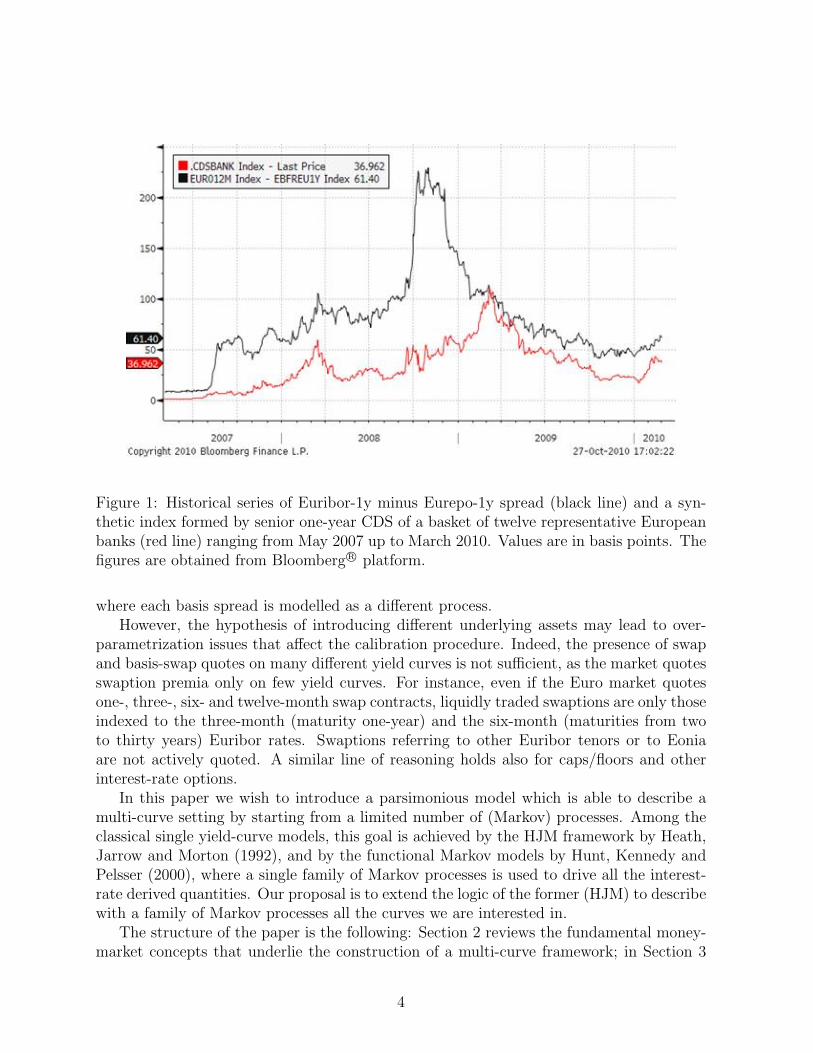
There are empirical studies supporting the idea that Libor rate levels cannot be utterlyjustified by counterparty credit risk arguments. In a European Central Bank workingpaper, Eisenschmidt and Tapking (2009) compare the spread of the Euribor over the generalcollateral repo rate to the spread of banking-sector credit default swaps of the same tenorduring the crisis period. Authors found that there is evidence of a large, persistent andtime varying component of the Euribor-Eurepo spread that cannot not be explained bycounterparty credit risk. In figure 1 we show the historical series of Euribor-Eurepo spreadfor a rate tenor of one year and of a synthetic index composed by senior one-year CDSspread of a basket of twelve European banks representative of the Libor panel. Surely thetwo series have some common qualitative characteristics. Yet, we find that the sharp rise inthe Euribor-Eurepo spread of September 2008 is only found three-four months later in theCDS spread series, confirming that a liquidity crisis needs time to evolve as credit crisis.Hence, counterparty risk is only one of the Libor dynamics driving factors, as discussed inHeideret al. (2009).
Recently in the literature some authors started to deal with these issues, mainly con-cerning the valuation of cross currency swaps as Boenkost and Schmidt (2005), Kijimaet al. (2009). In these papers, as in Henrard (2007, 2009), the problem is faced in apragmatic way by considering each forward rate as a single asset without investigating themicroscopical dynamics implied by liquidity and credit risks. Attempts in this differentdirection are made in Morini (2009), Morini and Prampolini (2010) and Fries (2010). Inparticular, we refer to Moreni and Morini (2010) where Libor rates of different tenors aremicroscopically associated to different short rates, which, in turn, are obtained by addingan instantaneous credit spread to the risk-free short rate.
Besides microscopic approaches, many authors extended yield-curve bootstrapping toa multi-curve setting, eventually resulting in new pricing models. These latters are ofteninspired by other asset classes, as Bianchetti (2009), Chibane and Sheldon (2009), Kijimaet al. (2009), Mercurio (2009), Martınez (2009), Kenyon (2010), or Pallavicini and Tarenghi(2010). We cite also a slightly different approach by Fujii et al. (2010) and Mercurio (2010),
where each basis spread is modelled as a different process.However, the hypothesis of introducing different underlying assets may lead to over-
parametrization issues that affect the calibration procedure. Indeed, the presence of swapand basis-swap quotes on many different yield curves is not sufficient, as the market quotesswaption premia only on few yield curves. For instance, even if the Euro market quotesone-, three-, six- and twelve-month swap contracts, liquidly traded swaptions are only thoseindexed to the three-month (maturity one-year) and the six-month (maturities from twoto thirty years) Euribor rates. Swaptions referring to other Euribor tenors or to Eoniaare not actively quoted. A similar line of reasoning holds also for caps/floors and otherinterest-rate options.
In this paper we wish to introduce a parsimonious model which is able to describe amulti-curve setting by starting from a limited number of (Markov) processes. Among theclassical single yield-curve models, this goal is achieved by the HJM framework by Heath,Jarrow and Morton (1992), and by the functional Markov models by Hunt, Kennedy andPelsser (2000), where a single family of Markov processes is used to drive all the interest-rate derived quantities. Our proposal is to extend the logic of the former (HJM) to describewith a family of Markov processes all the curves we are interested in.
The structure of the paper is the following: Section 2 reviews the fundamental money-market concepts that underlie the construction of a multi-curve framework; in Section 3
4
we describe an original extended HJM framework able to handle many yield curves; inSection 4, we detail a simple yet relevant specification (dubbed the Weighted GaussianModel) of the model that allows for simple evaluation of plain vanilla options, together withthe results of its calibration to market data; finally, Section 5 reviews our contributionsand hints for further developments.
2 Multi-curve relevant features
In order to motivate our modelling choices, it is useful to summarize the changes thatoccurred because of the credit crunch and the crucial issues a multi-curve framework shouldface. In this section we start identifying the risk-neutral measure, i.e. the risk-free discountterm-structure, with the one coming from Overnight Indexed Swaps (OIS), and then weintroduce risky rates (Libor). We also discuss, supporting our arguments with empiricalanalysis, the monotonicity properties of basis spreads and multi-tenor Libors.
2.1 Risk-free rates
First of all we assume that the market is arbitrage free, hence postulating the existence ofa risk-neutral measure. Under this measure every (risk-free) tradable asset instantaneouslyincreases its value at the risk-free rate rt. Furthermore, we introduce (risk-free) zero-couponbond prices and instantaneous forward rates as
Pt(T ) := Et
[−∫ T
t
du ru
]ft(T ) := ET
t [ rT ]
(1)
where the first expectation is taken under risk-neutral measure, and the last expectationis taken under a measure whose numeraire is Pt(T ) (hereafter simply T -forward measure).
As usual, we wish to link our risk-free rates to market quotes. In classical single-curveinterest-rate models, zero-coupon bond prices observed at time t = 0 form a term structure
T 7→ P0(T )
which can be made consistent with a selection of quotes (deposits, futures and interest-rateswaps). However, since the beginning of the crisis, many of them have been carrying arelevant amount of credit and/or liquidity risk and cannot be considered as belonging to therisk-neutral economy. Thus, the subset of the instruments to bootstrap the risk-free termstructure from has to be carefully chosen. A closer look at the Euro money market makesclear that quoted instruments are indexed on three reference indices1: Eonia, Euribor andEurepo.
1See European Banking Federation site at http://www.euribor-ebf.eu .
5
• Eonia is an effective rate calculated from the weighted average of all overnight unse-cured lending transactions undertaken in the interbank market.
• Euribor(s) are offered rates at which Euro interbank term deposits of different ma-turities are traded by one prime bank to another one.
• Eurepo(s) are offered rates at which Euro interbank secured money market transac-tions are traded.
Eonia and Euribor rates are unsecured, so that they incorporate the default risk ofthe counterparty of the transaction, while Eurepo rates are secured and free of credit risk.Thus, Eurepo rates could seem the natural proxy for risk-free rates2. The main issue withEurepo is that the longest quoted instrument has a maturity of one year. Longer maturitiesEuro money market deals are only indexed on Euribor and Eonia indices. In particular, wefound Eonia swap contracts (OIS) up to thirty years. Because of the plurality of availableOIS instruments and of the reduced credit/liquidity exposure on overnight deposits, tomany extent Eonia rates are the best available proxy for risk-free rates. This point has beenstressed by many authors, and we refer to Fujii et al. (2010) for more detailed arguments.
2.2 Libor rates
It is a common habit to refer to unsecured deposit rates over the period [t, T ] as Libor rates(Lt(T )). In this paper we follow this nomenclature and we reserve the term Euribor forthe index used as reference rate for deposits in the Euro area. As usual we can introducethe forward rates Ft(T, x) defined as
Ft(T, x) := ETt [LT−x(T ) ] . (2)
Forward rates Ft(T, x) are by construction martingales under the T -forward measure andeach of them represents the par rate seen at t for a swaplet accruing over [T − x, T ] andpaying at T a fixed rate in exchange for LT−x(T ).
Notice that accordingly to what said in the previous section, we consider one-day de-posits as being risk-free, while the longer the tenor, the greater will be the credit chargeon unsecured deposit rates. In other words we are thinking Eonia rates as (non-quoted)one-day-tenor Libor rates reducing as much as possible the deposit risks . By pushingthis analogy further we interpret Libor rates as microscopic rates at the same level of theshort-rate, and write
rt = limx→0
Lt(t+ x), (3)
which, given Eqs. (1) and (2), also reads
ft(T ) = limx→0
Ft(T, x). (4)
2See for instance Eisenshmidt and Tapking (2009) where the Euribor-Eurepo spread is used as anindicator of credit risk.
The usual no-arbitrage relationship between (risk-free) zero-coupon bond prices and Liborrates holds only for non-defaultable counterparties and instruments without liquidity risk.Hence, if Lt(x) is a Libor rate related to the period [t, t+ x], we get in general
Lt(t+ x) 6= 1
x
(1
Pt(t+ x)− 1
), ∀x > 0 .
Hence, when the presence of credit and liquidity risks invalidate the possibility of replicatingLibor indexed deposits with non-risky bonds Pt(T ), then interest-rate modelling shouldconsider Libor rates of different tenors as different assets. Yet, they should not move apartin a random way. At first glance, credit risk arguments imply that deposits with longertenor must be charged for a higher risk premium, so that, if the risk-free yield curve is nondecreasing, forward-rates should be a non-decreasing function of x.
For instance, let us consider the EUR money market and focus on the risk-free yieldcurve bootstrapped from Eonia indexed products, such as OIS up to one year of maturity.We identify risk-free linearly compounding rates with single-period OIS rates defined as
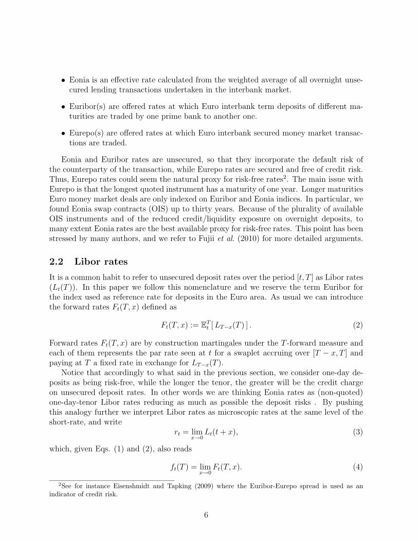
However, liquidity issues may invalidate such relationships. Actually let us recallthat both Eonia and Euribor rates refer to unsecured contracts, but Euribor rates donot represent effective transactions, while Eonia rate does. As an example of violations,we plot in figure 2 the daily historical values of spreads sE := E0(6m) − E0(3m) andsL = L0(6m)−L0(3m). We notice that in periods of great turmoil, as the last trimester of2007, even if the risk-free yield curve was often non-inverted, still the sL happened to benegative.
As a consequence, in the following we will not impose direct constraints on Libor orforward rates, focusing on relationships to link forward-rate volatilities.
2.2.2 Basis-swap spreads
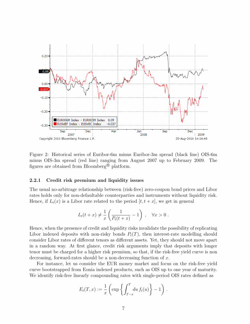
The starting point of our analysis was the raise of basis-swap spreads after the credit crisis.Once again simple credit risk arguments would require basis-swap spreads to be positive,but liquidity issues should also be considered. In the Euro area basis-swaps are quotedwith maturities ranging from one year up to thirty years, so that each leg contains a strip
8
of many Euribor rates. The averaging effect weakens the liquidity impact, but does notcancel it out. Indeed, in figure 3 we see that the basis-swap spread between one year andsix-month Euribor rates was often negative in the last trimester of 2009.
However, we find that in most cases quotes of basis-swap spreads are positive. In the lit-erature only Fujii et al. (2010) and Mercurio (2010) force constraints on basis-swap spreadsby direct modelling basis-swap spreads with respect to the EONIA rates with non-negativeprocesses, but this condition does not ensure that all quoted basis-swap spreads remainpositive.
Within our modeling framework, it will be quite difficult to impose constraints onbasis-swap spreads positivity, since we will not model them directly.
3 Extending the HJM framework
Our goal is to extend the classical HJM framework to include curves associated to differenttenors by modelling forward Libor rates by means of a common family of (Markov) pro-cesses. In the literature other authors proposed generalizations of the HJM framework, seefor instance Chiarella (2010) or Carmona (2004). In particular, in recent papers Martınez(2009) and Fujii (2010) extended the HJM framework to incorporate multiple-yield curvesand to deal with foreign currencies.
Our approach differs from the previous ones mainly on two relevant points. First, wemodel only observed rates as in Libor market model approaches, avoiding the introductionof quantities such as forecasting curve bonds or instantaneous rates. Second, we considera common family of processes for all the yield curves of a given currency, so that we areable to build parsimonious yet flexible models.
As a consequence of the discussion of previous sections, and in order to keep the modelas simple as possible, let us summarize the basic requirements the model must fulfill:
i) existence of a risk free curve, with instantaneous forward rates ft(T )
ii) existence of Libor rates, typical underlying of traded derivatives, with associatedforwards Ft(T, x)
iii) no arbitrage dynamics of the ft(T ) and the Ft(T, x) (both being T -forward measuremartingales) ensuring the limit case of Eq.(4)
iv) possibility of writing both the ft(T ) and the Ft(T, x) as function of a common familyof Markov processes.
While the first two requisites are related to the set of financial quantities we are about tomodel, the last two are conditions we impose on their dynamics, and will be granted by abefitting choice of model volatilities.
9
3.1 Generalized dynamics
According to requirements i) and ii) we model risk-free forward instantaneous rates ft(T )and (risky) forward Libor rates Ft(T, x), for which we choose, under the T−forward mea-sure, the following SDE3.
dft(T ) = σ∗t (T ) · dWt
d(k(T, x) + Ft(T, x))
(k(T, x) + Ft(T, x))= Σ∗t (T, x) · dWt
σt(T ) := σt(T ;T, 0)
Σt(T, x) :=
∫ T
T−xdu σt(u;T, x) ,
(5)
where we introduced the family of volatility (row) vector processes σt(u;T, x), the (row)vector of independent Brownian motions Wt, and the set of shifts k(T, x) that are requiredto satisfy4
limx→0
x k(T, x) = 1,
that is, k(T, x) ≈ 1/x if x ≈ 0.The identification of the volatility of risk free instantaneous forward rates ft(T ) withσt(T ;T, 0) is easily justified if we explicitly integrate the SDE for Ft(T, x)
Ft(T, x) = k(T, x)
((1 +
F0(T, x)
k(T, x)
)exp
{−1
2
∫ t
0
||Σs(T, x)| |2ds+
∫ t
0
Σ∗s(T, x) · dWs
}− 1
)and take the limit x → 0, such that Σs(T, x) ≈ xσs(T ;T, 0) +O(x2) and the exponentialmay be expanded in series of x.
The particular choice of a shifted forward Libor dynamics ensures the limit of Eq.(4)and is formally equivalent to the evolution of risk-free simple rates Et(T, x), which arefor instance shifted lognormal when standard HJM volatilities leads to an Hull and Whitemodel. In literature, direct modelling of shifted forward rates is also considered in Eberleinand Kluge (2007) (see also references therein), and in Papapantaleon (2010).
By means of the change of numeraire technique we have that
dW(T )t = dW
(rn)t − d
⟨W (rn), logP (T )
⟩t
= dW(rn)t +
(∫ T
t
duσt(u;u, 0)
)dt
where W (T ) and W (rn) are standard Brownian motions under T−forward and risk-neutralmeasure, respectively. It is then straightforward to write the dynamics of forward Libor
3See appendix A for vector and matrix notation.4This assumption may be generalized asking that k(T, x) ≈ φ(T, x)/x for a function φ such that
limx→0 φ(T, x) = 1.
10
rates and instantaneous risk-free rates under the risk neutral measure as
d(k(T, x) + Ft(T, x))
(k(T, x) + Ft(T, x))= Σ∗t (T, x) ·
[∫ T
t
du σt(u;u, 0)dt+ dWt
],
dft(T ) = σ∗t (T ) ·[∫ T
t
du σt(u;u, 0)dt+ dWt
] (6)
Wt being a risk-neutral measure multidimensional standard Brownian motion.
3.2 Constraints on the volatility process
Let us analyse more in detail the dynamics of the shifted forward Libors under risk-neutralmeasure. By integrating the SDE over the time period [0, t] we get
ln
(k(T, x) + Ft(T, x)
k(T, x) + F0(T, x)
)=
∫ t
0
Σ∗s(T, x) ·[dWs −
1
2Σs(T, x)ds+
∫ T
s
duσ∗s(u;u, 0)ds
].
To ensure the tractability and a Markovian specification of the model, we extend thesingle-curve HJM approach of Ritchken and Sankarasubramanian (1995), by setting
σt(u;T, x) := ht · q(u;T, x)g(t, u)
g(t, u) := exp
{−∫ u
t
dy λ(y)
}q(u;u, 0) = 1 ,
(7)
where h is a matrix adapted process, q is a diagonal matrix deterministic function (i.e. qij =qi1i=j) and λ is a deterministic array function. The condition on q when T = u is needed toensure that in the limit case x→ 0 we recover the standard Ritchen-Sankarasubramanianseparability condition.By plugging the expression for the volatility into Eq.(6), it is possible to work out theexpression ending up with the representation
ln
(k(T, x) + Ft(T, x)
k(T, x) + F0(T, x)
)=
G∗(t, T − x, T ;T, x) ·(Xt + Yt ·
(G0(t, t, T )− 1
2G(t, T − x, T ;T, x)
)), (8)
where we have defined the Ito stochastic process Xt
X it :=
N∑k=1
∫ t
0
gi(s, t)
(h∗ik,sdWk,s + (h∗shs)ik
∫ t
s
dy gk(s, y)ds
), i = 1, . . . , N
and the auxiliary matrix process Yt
Y ikt :=
∫ t
0
ds gi(s, t)(h∗shs)ikgk(s, t) i, k = 1, . . . , N
11
with X i0 = 0 and Y ik
0 = 0, as well as the vectorial deterministic functions
G0(t, T0, T1) :=
∫ T1
T0
dy g(t, y)
G(t, T0, T1;T, x) :=
∫ T1
T0
dy q(y;T, x)g(t, y) .
The limit case x→ 0, as previously detailed for general σt(u;T, x) still holds and we maycheck that ft(T ) = limx→0 Ft(T, x).
3.2.1 Dynamics of state variables
Equation (8) is the analogous of standard HJM reconstruction formula and is the mainresult of our paper. Let us notice that it returns a reconstruction formula for forward Liborrates, while standard HJM one is based on bonds. This important feature is consistentwith the requirement of a model capable to directly describe market relevant quantities.
Thanks to our assumption we are fully able to describe instantaneous forward rates(i.e. discounting curve bonds) and forward Libor rates once we know the state variables{Xt, Yt} , which satisfy, under the risk neutral measure, the following coupled (S)DE
dX it =
N∑k=1
(Y ikt − λi(t)X i
t
)dt+ h∗t · dWt
dY ikt =
[(h∗tht)ik − (λi(t) + λk(t))Y
ikt
]dt.
Let us notice that forward Libor diffusion pre-factors5 G(t, T−x, T ;T, x) depend on theq(u;T, x). This flexibility is a desirable feature, as it allows for a locally tuned dynamicsfor forward Libor rates, as we show in the next section.
3.2.2 Exact calibration and sensitivities
Our approach focuses on market quantities and leaves us the freedom of choosing theq(u;T, x) and the κ(T, x) such as to exactly calibrate a selection of market data. Thesefree parameters are independent from the skew/smile patterns that endogenously comewith the risk free HJM dynamics of Eonia single-period rates. This is a relevant advantageover other microscopic multi-curve models where the dynamics of microscopic quantitiesuniquely determines implied volatility patterns for rates of any tenor and maturity.
Thus, as relevant tenors and maturities form a discrete set (for instance x ∈ {1, 3, 6, 12}months), we may reasonably set κ(T, x) to be a piece-wise-constant deterministic function
5Actually, starting from (8), and switching to the terminal QT measure, we have
dFt(T, x) = [κ(T, x) + Ft(T, x)]G∗(t, T − x, T ;T, x) · h∗t · dWt .
12
to be exactly calibrated to a subset of caplet or swaption skews. Further, we have the samepossibility for a subset of at-the-money caplet or swaption volatilities by properly definingthe q(u;T, x) process.
For instance, it is possible to set
q(u;T, x) := q(T, x)p(u) ,
with q a scalar function and p an array function. With this prescription q may be usedto exactly calibrate a subset of at-the-money quotes, while the array p allows to select thesubset of the X that is relevant for the diffusion of Ft(T, x). In this way we may associatethe dynamics of a chosen rate to a selection of relevant “diffusion modes”.
The possibility of an exact calibration to a subset of at-the-money caplet or swaptionvolatilities and skews easily allows for sensitivity computation, and is similar to whathappens in stochastic local volatility models, see for instance Torrealba (2010), where,after having calibrated the parameters of the volatility process, the local term allows foran exact calibration to some relevant market quotes.
3.3 Eonia simple rates
For sake of completeness we may also compute Eonia simple rates Et(T, x) by plugging theseparable volatility form within the relationship
1 + xEt(T, x) = exp
{∫ T
T−xdy ft(y)
}such that
ln
(1 + xEt(T, x)
1 + xE0(T, x)
)=
G∗0(t, T − x, T ) ·(Xt + Yt ·
(G0(t, t, T )− 1
2G0(t, T − x, T )
)). (9)
Let us notice that if we set q(u;T, x) ≡ 1, then G0(t, T − x, T ) ≡ G(t, T − x, T, x, T )such that Ft(T, x) and Et(T, x) would differ only in their shifts and initial values. Ifwe moreover choose κ(T, x) = 1/x, we would obtain a model with perfect instantaneouscorrelation between Libors and Eonia simple rates in which
1 + xFt(T, x)
1 + xEt(T, x)=
1 + xF0(T, x)
1 + xE0(T, x),
hence showing that the static correction model of Henrard (2009) is a particular case ofthis extended HJM framework.
13
3.4 Swap rates
Our framework also allows us to derive an (approximated) expression for swap rates dy-namics.Let us consider a swap with a x tenor floating leg and a x tenor fixed one paying at times{Ta+1, . . . , Tb} and {Ta+1, . . . , Tb}, respectively. The swap par rate equating the two legs is
Sabt (x, x) :=
∑bk=a+1 τkPt(Tk)Ft(Tk, x)∑b
k=a+1 τkPt(Tk)
where the quantities with a bar refer to the fix leg. We introduce the weights w as
wabk (t)(x, x) :=τkPt(Tk)∑b
k=a+1 τkPt(Tk)
and perform the usual freezing (see Errais and Mercurio (2005)) technique to obtain, underthe swap measure Qab,
dSabt (x, x) ≈b∑
k=a+1
wabk (t)dFt(Tk, x)
=b∑
k=a+1
wabk (t) [κ(Tk, x) + Ft(Tk, x)] Σ∗t (Tk, x) · dWt
≈(Sabt (x, x) + ψab(x, x)
) b∑k=a+1
δabk Σ∗t (Tk, x) · dWt ,
where
ψab(x, x) :=
∑bk=a+1 τkP0(Tk)κ(Tk, x)∑b
j=a+1 τjP0(Tj)
δabk (x) :=τkPt(Tk)(κ(Tk, x) + F0(Tk, x))∑b
j=a+1 τjPt(Tj)(κ(x, Tj) + F0(x, Tj)).
With similar arguments we get an expression also for basis swap spreads, since we have
Babt (x, x′) =: Sabt (x, x′)− Sabt (x′, x′) .
3.5 Volatility dynamics
As in the single-curve HJM framework we can add a stochastic volatility process to ourmodel by extending the filtration to include also the information generated by the volatilityprocess. A popular choice is to model the matrix process ht by means of a square-rootprocess (see for instance Trolle and Schwartz (2009) and reference therein).
14
We start by replacing the ht process by
ht :=√vtR
∗
where R is a lower triangular matrix, while the variance vt is a vector process whosedynamics under risk neutral measure is given by
dvt = κ (θ − vt) dt+ ν√vt dZt , v0 = v
where κ,θ,ν,v are constant deterministic vectors, and Zt is a vector of independent Brow-nian motions correlated to the Wt processes as given by
ρii dt := d〈Z,Wi〉t , and ρij = 0 for i 6= j
where ρ is a diagonal deterministic correlation matrix.With this choice we get shifted Heston dynamics for market rates, so that we can
calculate option pricing with usual Fourier transform techniques (see Lewis (2001)).
4 Model calibration and numerical examples
As shown in Pallavicini and Tarenghi (2010) there are evidences that the money marketfor Euro area has moved to a multi-curve setting for what concerns the pricing of plain-vanilla instruments like interest-rate swaps, but the situation is not so clear for derivativecontracts, where the calibration of volatility and correlation parameters may hide theimpact of which yield curve is used in pricing. In particular, this holds for CMS swapsand CMS options, while the swaption market has evidences of pricing in the old single-curve approach, although some contributors start quoting in multi-curve framework fromSeptember 2010.
On the other hand, the money market for Euro area does not quote options on all ratetenors. In Euro area only options on the six-months tenor are widely listed, while the three-months tenor is present only in few quotes (swaptions with one-year tenor and cap/floorswith maturities up to two years), and options on the other rate tenors are missing. Thus,any model which requires a different dynamics for each term-structure, has the problemthat market quotes cannot be found to fix all its degrees of freedom.
In particular, we consider a simple extension of a two-factor Gaussian model (see G2++model in Brigo and Mercurio (2006)), that we call Weighted Gaussian model (WG2++model), since the terms depending on Libor tenors appear as multiplicative weights of the
15
X processes. Notice that we could use more than two factors (WGn++ model), or wecould add stochastic volatility to calibrate also the swaption volatility smile, leading to aWeighted Heston model (WHn++ model).
4.1 The Weighted Gaussian model
As an example we introduce a simple specification of our generic HJM multi-curve ap-proach, with different dynamics for each forward Libor rate. In practice it is a generaliza-tion of a shifted n-factor Hull and White model associated to risk-free rates.Let us set the volatility process ht to be in the form
ht := ε(t)hR∗ ,
where h is a diagonal constant matrix hij = hiδi=j, R is a lower triangular matrix repre-senting the pseudo-square root of a correlation matrix ρ, and we allow for a time varyingcommon volatility shape in the form
ε(t) := 1 + (β0 − 1 + β1t)e−β2t ,
where β0, β1, β2 are three positive constants. Microscopical Markov factors X and Y evolveunder the risk free measure, as
dX it =
(n∑j=1
Y ijt − λiX i
t
)dt+ ε(t)hidW
it
dY ijt =
(ε2(t)hihjρij + (λi + λj)Y
ijt
)dt
d〈W iW j〉t = ρijdt
(10)
where the λi are non negative constants, and dWt := R∗ · dWt.The risk free short rate is given as usual by
rt := f0(t) +n∑k=1
X it
and the shift term f0(t) allows to recover t = 0 risk free yield curve6.As for the tenor-maturity factors q, we chose a maturity independent form of the type
qi(u;T, x) := e−xηi .
Numerical tests are done with n = 2, hence leading to ten free parameters
{λ1, λ2, h1, h2, η1, η2, ρ12, β0, β1, β2} ,
and for sake of simplicity we set κ(T, x) = 1/x.By construction this model supports different forecasting curves and we bootstrappedinitial forward Libors F0(T, x) by means of the Eonia term structure (discounting) anddifferent tenors Euribor term structures.
6As the Y are deterministic, this model is often written by explicitly computing the Y -related quantitiessuch as the drift of the X. Those quantities are then incorporated into a generic shift.
Table 1: Eonia term-structure expressed in term of ACT/360 zero-rates and Euribor termstructures for three- six- month tenors expressed in terms of ACT/360 forward rates.Bootstrapping details can be found on Pallavicini and Tarenghi (2010). Data bootstrappedfrom market quotes observed on 12 of August 2010.
4.2 Benchmark models
In our numerical examples we compare the results of the WG2++ model with respect toother two HJM-like models, all with two driving factors and time-dependent volatilities.We discount flows by means of the Eonia term structure and use for forecasting purposesthe Euribor term structures.
• The G2++ model of Brigo and Mercurio (2006). This is a single-curve (old-style)model which we extend to incorporate time-dependent volatilities via the commontime-dependent factor ε(t). It is obtained by setting ηj ≡ 0, (i.e. q ≡ 1,) andF0(T, x) ≡ E0(T, x). For this model we use, as discounting and forwarding curve,a term structure obtained with old-style standard techniques from deposits, futuresand swap rates.
• The MMG model of Pallavicini and Tarenghi (2010). This is an uncertain parametermulti-curve model which we restrict to have only one scenario. It is obtained bysetting ηj ≡ 0, uses separate forwarding and discounting curves and, as discussed inSect.3.3, reduces to Henrard static correction model. It has eight free parameters(λ1,h1,λ2,h2,ρ12,β0,β1,β2) and uses the same curves as the Weighted Gaussian.
The initial yield curves can be bootstrapped from the money market quotes. We refer againto Pallavicini and Tarenghi (2010) and references therein for a complete discussion. Here,we adopt their methodology. In particular we use the Eonia term-structure to discountcash flows, as a proxy for the risk-free yield curve (see also Fujii et al. (2010) and Mercurio(2010)).
In table 1 we show the Eonia term-structure expressed in term of ACT/360 zero-rates,and the Euribor term structures for three- six- month tenors expressed in terms of ACT/360forward rates.
4.4 Swaption pricing formula
Swaption prices are given by the following expectation value under risk-neutral measure
Πabt := Et
[exp
{−∫ Ta
t
du ru
}Aab(Ta; x)(Sab(Ta;x, x)−K)+
]Under the approximation of Section 3.4, which is pretty good for ATM swaptions, we geta log-shifted dynamics for swap rates such that
In table 3 we list the model parameters obtained from the calibration procedure. Noticethat the two driving processes X1
t and X2t operate on two different time scales. Indeed, by
construction the first process has always a speed of mean reversion smaller than the oneof the second process. This constraint is enforced while calibrating to avoid a degenerateproblem.
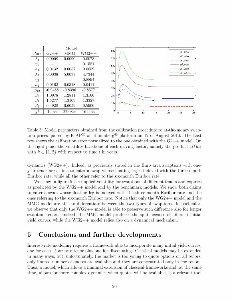
In the figure on the right side of table 2 the volatility backbones of each driving factor,namely the product ε(t)hk with k ∈ {1, 2} plotted with respect to time t in years. Wecan see that, allowing for more degrees of freedom along the Euribor tenor space as weincrease the complexity of the model, the volatilities of the two driving processes X1
t andX2t split apart: a higher volatility for the process with higher speed of mean reversion
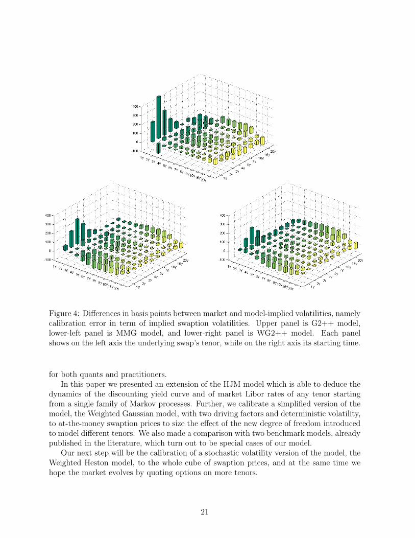
(process acting on a shorter time scale).Calibration errors in term of implied swaption volatilities are shown in figure 4. We
can see that the calibration error for swaptions with a tenor of one year is less as long asthe model allows for incorporating multiple yield curves (MMG) and differentiating their
dynamics (WG2++). Indeed, as previously stated in the Euro area swaptions with one-year tenor are claims to enter a swap whose floating leg is indexed with the three-monthEuribor rate, while all the other refer to the six-month Euribor rate.
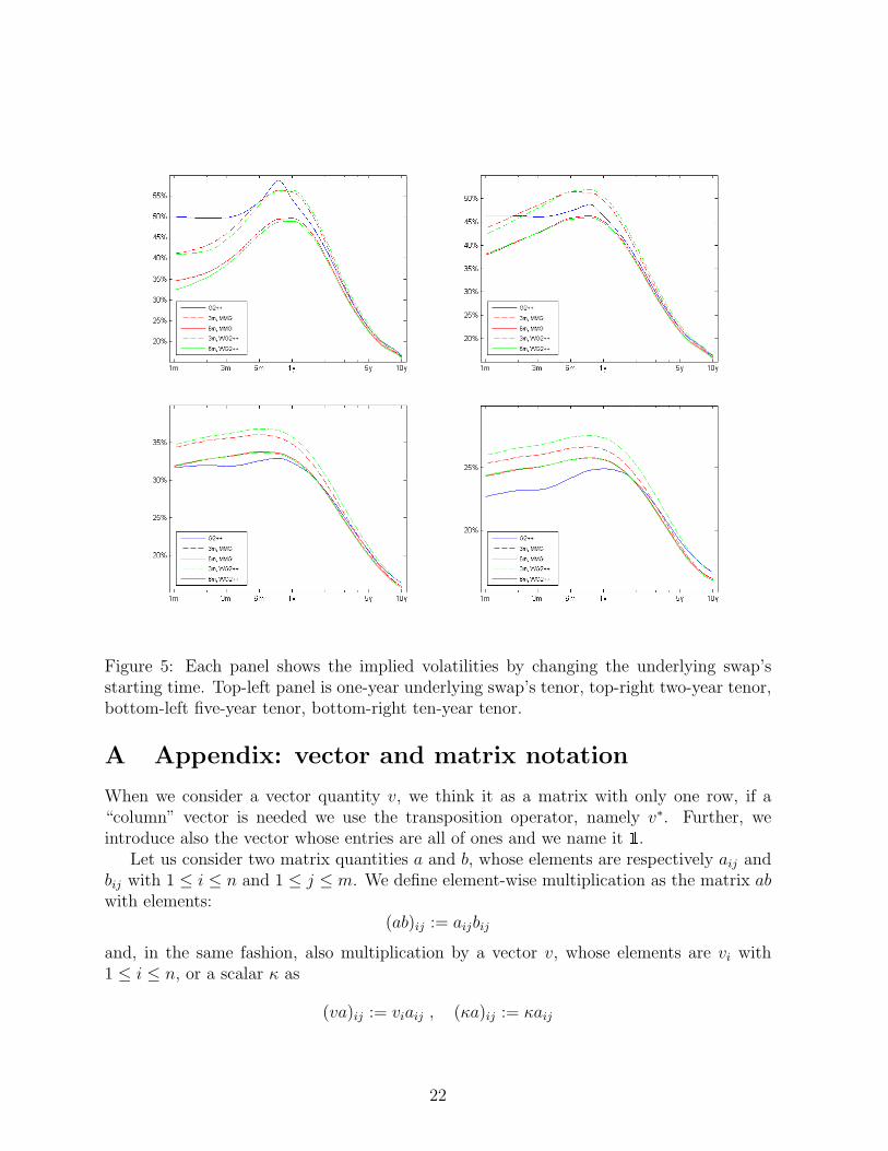
We show in figure 5 the implied volatility for swaptions of different tenors and expiriesas predicted by the WG2++ model and by the benchmark models. We show both claimsto enter a swap whose floating leg is indexed with the three-month Euribor rate and theones referring to the six-month Euribor rate. Notice that only the WG2++ model and theMMG model are able to differentiate between the two types of swaptions. In particular,we observe that only the WG2++ model is able to preserve such difference also for longerswaption tenors. Indeed, the MMG model produces the split because of different initialyield curves, while the WG2++ model relies also on a dynamical mechanism.
5 Conclusions and further developments
Interest-rate modelling requires a framework able to incorporate many initial yield curves,one for each Libor rate tenor plus one for discounting. Classical models may be extendedin many ways, but, unfortunately, the market is too young to quote options on all tenors:only limited number of quotes are available and they are concentrated only in few tenors.Thus, a model, which allows a minimal extension of classical frameworks and, at the sametime, allows for more complex dynamics when quotes will be available, is a relevant tool
20
Figure 4: Differences in basis points between market and model-implied volatilities, namelycalibration error in term of implied swaption volatilities. Upper panel is G2++ model,lower-left panel is MMG model, and lower-right panel is WG2++ model. Each panelshows on the left axis the underlying swap’s tenor, while on the right axis its starting time.
for both quants and practitioners.In this paper we presented an extension of the HJM model which is able to deduce the
dynamics of the discounting yield curve and of market Libor rates of any tenor startingfrom a single family of Markov processes. Further, we calibrate a simplified version of themodel, the Weighted Gaussian model, with two driving factors and deterministic volatility,to at-the-money swaption prices to size the effect of the new degree of freedom introducedto model different tenors. We also made a comparison with two benchmark models, alreadypublished in the literature, which turn out to be special cases of our model.
Our next step will be the calibration of a stochastic volatility version of the model, theWeighted Heston model, to the whole cube of swaption prices, and at the same time wehope the market evolves by quoting options on more tenors.
21
Figure 5: Each panel shows the implied volatilities by changing the underlying swap’sstarting time. Top-left panel is one-year underlying swap’s tenor, top-right two-year tenor,bottom-left five-year tenor, bottom-right ten-year tenor.
A Appendix: vector and matrix notation
When we consider a vector quantity v, we think it as a matrix with only one row, if a“column” vector is needed we use the transposition operator, namely v∗. Further, weintroduce also the vector whose entries are all of ones and we name it 1.
Let us consider two matrix quantities a and b, whose elements are respectively aij andbij with 1 ≤ i ≤ n and 1 ≤ j ≤ m. We define element-wise multiplication as the matrix abwith elements:
(ab)ij := aijbij
and, in the same fashion, also multiplication by a vector v, whose elements are vi with1 ≤ i ≤ n, or a scalar κ as
(va)ij := viaij , (κa)ij := κaij
22
while index contraction as the matrix a∗ · b with elements:
(a∗ · b)jk :=n∑i=1
aijbik
References
[1] M. Bianchetti (2009). Two Curves, One Price: Pricing ad Hedging Interest RateDerivatives Using Different Yield Curves for Discounting and Forwarding. Availableat http://ssrn.com/abstract=1334356.
[2] M. Bianchetti (2010). Multiple Curves, One Price: The Post Credit-Crunch InterestRate Market. Talk kept at “Risk and modelling fixed income interest rates”, MarcusEvans conference, London, 15-16 April.
[3] W. Boenkost and W.M. Schmidt (2005). Cross currency swap valuation. Available athttp://ssrn.com/abstract=1375540.
[4] D. Brigo, and F. Mercurio (2006). Interest Rate Models: Theory and Practice – withSmile, Inflation and Credit, Second Edition, Springer Verlag.
[5] R. Carmona (2004). HJM: a Unified Approach to Dynamic Models for Fixed Income,Credit and Equity Markets. in Paris-Princeton Lectures on Mathematical Finance2004, Springer.
[6] C. Chiarella, S.C. Maina and C. Nikitipoulos Sklibosios, (2010). Markovian Default-able HJM Term Structure Models with Unspanned Stochastic Volatility. Available athttp://ssrn.com/abstract=1695295.
[7] M. Chibane and G. Sheldon (2009). Building Curves on a Good Basis. Available athttp://ssrn.com/abstract=1394267.
[8] E. Eberlein, and W. Kluge (2007). Calibration of Levy term structure models. InM. Fu, R. A. Jarrow, J.-Y. Yen, and R. J. Elliott (Eds.), Advances in MathematicalFinance: In Honor of Dilip B. Madan, pg. 155–180. Birkhauser.
[9] J. Eisenschimdt and J. Tapking (2009). Liquidity Risk Premia in Unsecured InterbankMoney Markets. ECB Working Paper Series, 1025, 3.
[10] E. Errais and F. Mercurio (2005). Yes, Libor Models can Capture Inter-est Rate Derivatives Skew: A Simple Modelling Approach. Available athttp://ssrn.com/abstract=680621
[11] C. Fries (2010). Discounting Revisited: valuation under funding, counterparty riskand collateralization (2010). Available at http://ssrn.com/abstract=1609587
23
[12] E. Fruchard, C. Zammouri and E. Willems (1995). Basis for change, Risk, Vol. 8,No.10 , 70-75, October.
[13] M. Fujii, Y. Shimada and A. Takahashi (2010). On the Term Structure of In-terest Rates with Basis Spreads, Collateral and Multiple Currencies. Available athttp://ssrn.com/abstract=1556487
[14] P. Hunt, J. Kennedy, and A. Pelsser (2000) Markov-functional interest rate models,Finance and Stochastics, Springer, vol. 4(4), pages 391-408.
[15] D. Heath, R. Jarrow, A. Morton (1992). Bond Pricing and the Term Structure ofInterest Rates: a new methodology. Econometrica 60, 77-105.
[16] M. Henrard, M. (2007). The Irony in the Derivatives Discounting. Wilmott Magazine,July 2007, 92-98.
[17] M. Henrard (2009). The Irony in the Derivatives Discounting Part II: The Crisis.Preprint, Dexia Bank, Brussels.
[18] C. Kenyon (2010). Short-Rate Pricing after the Liquidity and Credit Shocks: Includingthe Basis. Available at http://ssrn.com/abstract=1558429
[19] M. Kijima, K. Tanaka and T. Wong (2009). A Multi-Quality Model of Interest Rates,Quantitative Finance 9(2), 133-145.
[20] A. Lewis (2001). A simple option formula for general jump-diffusion and other expo-nential Levy processes. Available at http://ssrn.com/abstract=282110.
[21] T. Martınez (2009). Drift conditions on a HJM model with stochastic basis spreads.Available at http://www.risklab.es/es/jornadas/2009/index.html
[22] F. Mercurio (2009). Interest Rates and The Credit Crunch: New Formulas and MarketModels. Bloomberg Portfolio Research Paper No. 2010-01-FRONTIERS. Available athttp://ssrn.com/abstract=1332205
[23] F. Mercurio (2010). LIBOR Market Models with Stochastic Basis. Available athttp://ssrn.com/abstract=1563685
[24] N.Moreni and M. Morini (2010). A note on multiple curve term structure modelingwith credit/liquidity spread, Banca IMI Internal Report.
[25] M. Morini (2009). Solving the Puzzle in the Interest Rate Market. Available athttp://ssrn.com/abstract=1506046
[26] M. Morini and A. Prampolini (2010). Risky Funding: A unified framework for coun-terparty and liquidity charges. Available at http://www.defaultrisk.com
24
[27] A. Papapantaleon (2010).Old and New Approaches to Libor Modeling.Statistica Neer-landica 64, 3.
[28] A. Pallavicini and M. Tarenghi (2010). Interest-Rate Modeling with Multiple YieldCurves. Available at http://ssrn.com/abstract=1629688
[29] P. Ritchken and L. Sankarasubramanian (1995). Volatility Structures of Forward Ratesand the Dynamics of the Term Structure. Mathematical Finance 7, 157-176.
[30] M. Torrealba (2010). Modelling the Spread and Applications to Callable Spread Op-tions. Talk presented at 6th WBS Fixed Income Conference, Madrid 2010.
[31] A. Trolle and E. Schwartz (2009). A General Stochastic Volatility Model for the Pricingof Interest Rate Derivatives. Review of Financial Studies, vol. 22(5), pages 2007-2057.