133
Part 3 General Relativity Harvey Reall
Part 3 General Relativity
Harvey Reall

Part 3 GR December 1, 2017 ii H.S. Reall
Contents
Preface vii
1 Equivalence Principles 11.1 Incompatibility of Newtonian gravity and Special Relativity . . . . 11.2 The weak equivalence principle . . . . . . . . . . . . . . . . . . . . 21.3 The Einstein equivalence principle . . . . . . . . . . . . . . . . . . . 41.4 Tidal forces . . . . . . . . . . . . . . . . . . . . . . . . . . . . . . . 41.5 Bending of light . . . . . . . . . . . . . . . . . . . . . . . . . . . . . 51.6 Gravitational red shift . . . . . . . . . . . . . . . . . . . . . . . . . 61.7 Curved spacetime . . . . . . . . . . . . . . . . . . . . . . . . . . . . 8
2 Manifolds and tensors 112.1 Introduction . . . . . . . . . . . . . . . . . . . . . . . . . . . . . . . 112.2 Differentiable manifolds . . . . . . . . . . . . . . . . . . . . . . . . 122.3 Smooth functions . . . . . . . . . . . . . . . . . . . . . . . . . . . . 152.4 Curves and vectors . . . . . . . . . . . . . . . . . . . . . . . . . . . 162.5 Covectors . . . . . . . . . . . . . . . . . . . . . . . . . . . . . . . . 202.6 Abstract index notation . . . . . . . . . . . . . . . . . . . . . . . . 222.7 Tensors . . . . . . . . . . . . . . . . . . . . . . . . . . . . . . . . . 222.8 Tensor fields . . . . . . . . . . . . . . . . . . . . . . . . . . . . . . . 272.9 The commutator . . . . . . . . . . . . . . . . . . . . . . . . . . . . 282.10 Integral curves . . . . . . . . . . . . . . . . . . . . . . . . . . . . . 29
3 The metric tensor 313.1 Metrics . . . . . . . . . . . . . . . . . . . . . . . . . . . . . . . . . . 313.2 Lorentzian signature . . . . . . . . . . . . . . . . . . . . . . . . . . 343.3 Curves of extremal proper time . . . . . . . . . . . . . . . . . . . . 36
4 Covariant derivative 394.1 Introduction . . . . . . . . . . . . . . . . . . . . . . . . . . . . . . . 394.2 The Levi-Civita connection . . . . . . . . . . . . . . . . . . . . . . . 43
iii
CONTENTS
4.3 Geodesics . . . . . . . . . . . . . . . . . . . . . . . . . . . . . . . . 45
4.4 Normal coordinates . . . . . . . . . . . . . . . . . . . . . . . . . . . 47
5 Physical laws in curved spacetime 49
5.1 Minimal coupling, equivalence principle . . . . . . . . . . . . . . . . 49
5.2 Energy-momentum tensor . . . . . . . . . . . . . . . . . . . . . . . 51
6 Curvature 55
6.1 Parallel transport . . . . . . . . . . . . . . . . . . . . . . . . . . . . 55
6.2 The Riemann tensor . . . . . . . . . . . . . . . . . . . . . . . . . . 56
6.3 Parallel transport again . . . . . . . . . . . . . . . . . . . . . . . . 57
6.4 Symmetries of the Riemann tensor . . . . . . . . . . . . . . . . . . 59
6.5 Geodesic deviation . . . . . . . . . . . . . . . . . . . . . . . . . . . 60
6.6 Curvature of the Levi-Civita connection . . . . . . . . . . . . . . . 62
6.7 Einstein’s equation . . . . . . . . . . . . . . . . . . . . . . . . . . . 63
7 Diffeomorphisms and Lie derivative 67
7.1 Maps between manifolds . . . . . . . . . . . . . . . . . . . . . . . . 67
7.2 Diffeomorphisms, Lie Derivative . . . . . . . . . . . . . . . . . . . . 69
8 Linearized theory 77
8.1 The linearized Einstein equation . . . . . . . . . . . . . . . . . . . . 77
8.2 The Newtonian limit . . . . . . . . . . . . . . . . . . . . . . . . . . 80
8.3 Gravitational waves . . . . . . . . . . . . . . . . . . . . . . . . . . . 83
8.4 The field far from a source . . . . . . . . . . . . . . . . . . . . . . . 88
8.5 The energy in gravitational waves . . . . . . . . . . . . . . . . . . . 92
8.6 The quadrupole formula . . . . . . . . . . . . . . . . . . . . . . . . 96
8.7 Comparison with electromagnetic radiation . . . . . . . . . . . . . . 98
8.8 Gravitational waves from binary systems . . . . . . . . . . . . . . . 100
9 Differential forms 105
9.1 Introduction . . . . . . . . . . . . . . . . . . . . . . . . . . . . . . . 105
9.2 Connection 1-forms . . . . . . . . . . . . . . . . . . . . . . . . . . . 106
9.3 Spinors in curved spacetime . . . . . . . . . . . . . . . . . . . . . . 109
9.4 Curvature 2-forms . . . . . . . . . . . . . . . . . . . . . . . . . . . . 111
9.5 Volume form . . . . . . . . . . . . . . . . . . . . . . . . . . . . . . . 112
9.6 Integration on manifolds . . . . . . . . . . . . . . . . . . . . . . . . 114
9.7 Submanifolds and Stokes’ theorem . . . . . . . . . . . . . . . . . . . 115
Part 3 GR December 1, 2017 iv H.S. Reall
CONTENTS
10 Lagrangian formulation 11910.1 Scalar field action . . . . . . . . . . . . . . . . . . . . . . . . . . . . 11910.2 The Einstein-Hilbert action . . . . . . . . . . . . . . . . . . . . . . 12010.3 Energy momentum tensor . . . . . . . . . . . . . . . . . . . . . . . 123
Part 3 GR December 1, 2017 v H.S. Reall

CONTENTS
Part 3 GR December 1, 2017 vi H.S. Reall
Preface
These are lecture notes for the course on General Relativity in Part III of theCambridge Mathematical Tripos. There are introductory GR courses in Part II(Mathematics or Natural Sciences) so, although self-contained, this course does notcover topics usually covered in a first course, e.g., the Schwarzschild solution, thesolar system tests, and cosmological solutions. You should consult an introductorybook (e.g. Gravity by J.B. Hartle) if you have not studied these topics before.
Acknowledgment
I am very grateful to Andrius Stikonas for producing the figures.
Conventions
Apart from the first lecture, we will use units in which the speed of light is one:c = 1.
We will use ”abstract indices” a, b, c etc to denote tensors, e.g. V a, gcd. Equa-tions involving such indices are basis-independent. Greek indices µ, ν etc refer totensor components in a particular basis. Equations involving such indices are validonly in that basis.
We will define the metric tensor to have signature (−+++), which is the mostcommon convention. Some authors use signature (+−−−).
Our convention for the Riemann tensor is such that the Ricci identity takesthe form
∇a∇bVc −∇b∇aV
c = RcdabV
d.
Some authors define the Riemann tensor with the opposite sign.
vii
CHAPTER 0. PREFACE
Bibliography
There are many excellent books on General Relativity. The following is an incom-plete list:
1. General Relativity, R.M. Wald, Chicago UP, 1984.
2. Advanced General Relativity, J.M. Stewart, CUP, 1993.
3. Spacetime and geometry: an introduction to General Relativity, S.M. Carroll,Addison-Wesley, 2004.
4. Gravitation, C.W. Misner, K.S. Thorne and J.A. Wheeler, Freeman 1973.
5. Gravitation and Cosmology, S. Weinberg, Wiley, 1972.
Our approach will be closest to that of Wald. The first part of Stewart’s bookis based on a previous version of this course. Carroll’s book is a very readableintroduction. Weinberg’s book contains a good discussion of equivalence principles.Our treatments of the Newtonian approximation and gravitational radiation arebased on Misner, Thorne and Wheeler.
Part 3 GR December 1, 2017 viii H.S. Reall
Chapter 1
Equivalence Principles
1.1 Incompatibility of Newtonian gravity and Spe-
cial Relativity
Special relativity has a preferred class of observers: inertial (non-accelerating)observers. Associated to any such observer is a set of coordinates (t, x, y, z) calledan inertial frame. Different inertial frames are related by Lorentz transformations.The Principle of Relativity states that physical laws should take the same form inany inertial frame.
Newton’s law of gravitation is
∇2Φ = 4πGρ (1.1)
where Φ is the gravitational potential and ρ the mass density. Lorentz transforma-tions mix up time and space coordinates. Hence if we transform to another inertialframe then the resulting equation would involve time derivatives. Therefore theabove equation does not take the same form in every inertial frame. Newtoniangravity is incompatible with special relativity.
Another way of seeing this is to look at the solution of (1.1):
Φ(t,x) = −G∫d3y
ρ(t,y)
|x− y|(1.2)
From this we see that the value of Φ at point x will respond instantaneously toa change in ρ at point y. This violates the relativity principle: events which aresimultaneous (and spatially separated) in one inertial frame won’t be simultaneousin all other inertial frames.
The incompatibility of Newtonian gravity with the relativity principle is nota problem provided all objects are moving non-relativistically (i.e. with speeds
1
CHAPTER 1. EQUIVALENCE PRINCIPLES
much less than the speed of light c). Under such circumstances, e.g. in the SolarSystem, Newtonian theory is very accurate.
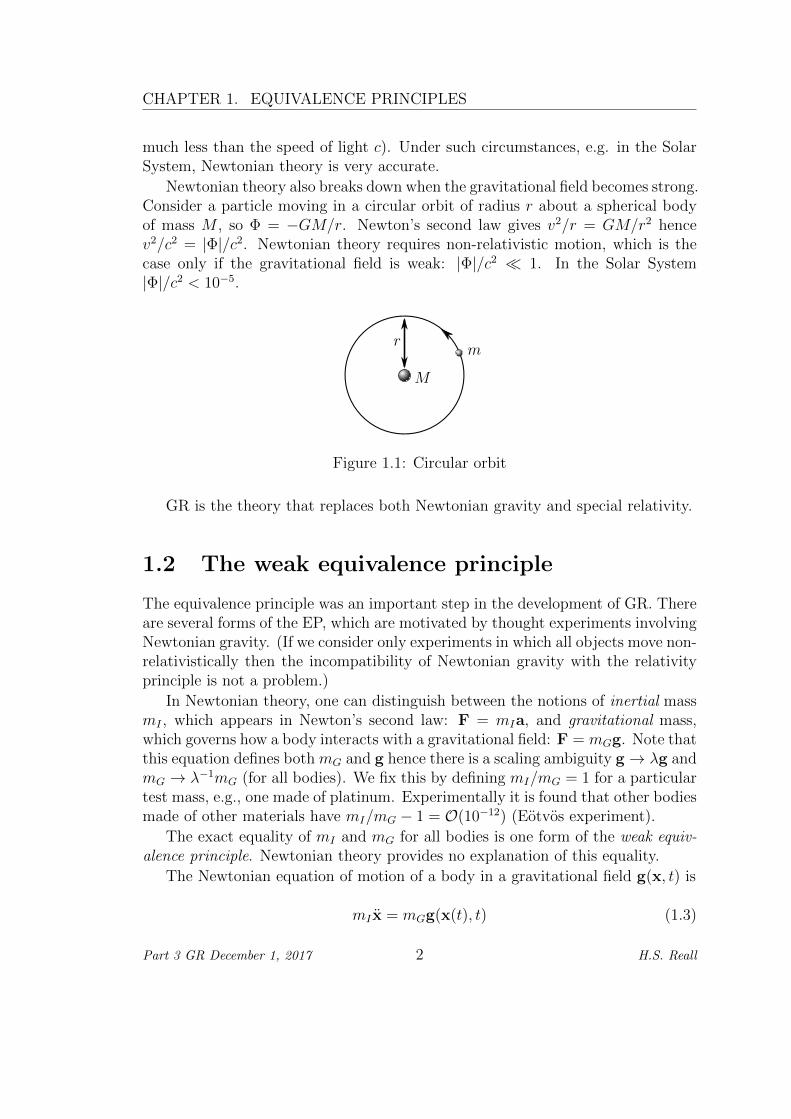
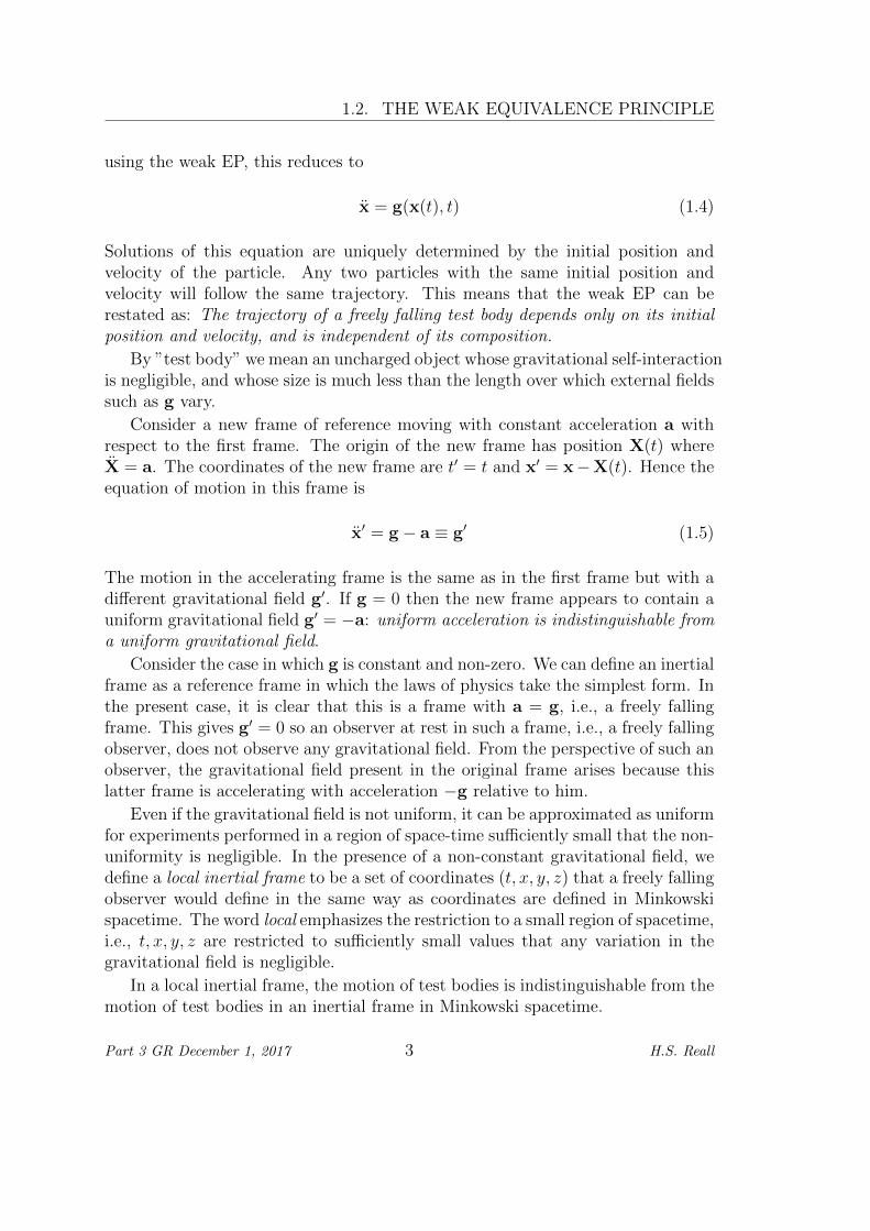
Newtonian theory also breaks down when the gravitational field becomes strong.Consider a particle moving in a circular orbit of radius r about a spherical bodyof mass M , so Φ = −GM/r. Newton’s second law gives v2/r = GM/r2 hencev2/c2 = |Φ|/c2. Newtonian theory requires non-relativistic motion, which is thecase only if the gravitational field is weak: |Φ|/c2 1. In the Solar System|Φ|/c2 < 10−5.
M
mr
Figure 1.1: Circular orbit
GR is the theory that replaces both Newtonian gravity and special relativity.
1.2 The weak equivalence principle
The equivalence principle was an important step in the development of GR. Thereare several forms of the EP, which are motivated by thought experiments involvingNewtonian gravity. (If we consider only experiments in which all objects move non-relativistically then the incompatibility of Newtonian gravity with the relativityprinciple is not a problem.)
In Newtonian theory, one can distinguish between the notions of inertial massmI , which appears in Newton’s second law: F = mIa, and gravitational mass,which governs how a body interacts with a gravitational field: F = mGg. Note thatthis equation defines both mG and g hence there is a scaling ambiguity g→ λg andmG → λ−1mG (for all bodies). We fix this by defining mI/mG = 1 for a particulartest mass, e.g., one made of platinum. Experimentally it is found that other bodiesmade of other materials have mI/mG − 1 = O(10−12) (Eotvos experiment).
The exact equality of mI and mG for all bodies is one form of the weak equiv-alence principle. Newtonian theory provides no explanation of this equality.
The Newtonian equation of motion of a body in a gravitational field g(x, t) is
mI x = mGg(x(t), t) (1.3)
Part 3 GR December 1, 2017 2 H.S. Reall
1.2. THE WEAK EQUIVALENCE PRINCIPLE
using the weak EP, this reduces to
x = g(x(t), t) (1.4)
Solutions of this equation are uniquely determined by the initial position andvelocity of the particle. Any two particles with the same initial position andvelocity will follow the same trajectory. This means that the weak EP can berestated as: The trajectory of a freely falling test body depends only on its initialposition and velocity, and is independent of its composition.
By ”test body” we mean an uncharged object whose gravitational self-interactionis negligible, and whose size is much less than the length over which external fieldssuch as g vary.
Consider a new frame of reference moving with constant acceleration a withrespect to the first frame. The origin of the new frame has position X(t) whereX = a. The coordinates of the new frame are t′ = t and x′ = x−X(t). Hence theequation of motion in this frame is
x′ = g − a ≡ g′ (1.5)
The motion in the accelerating frame is the same as in the first frame but with adifferent gravitational field g′. If g = 0 then the new frame appears to contain auniform gravitational field g′ = −a: uniform acceleration is indistinguishable froma uniform gravitational field.
Consider the case in which g is constant and non-zero. We can define an inertialframe as a reference frame in which the laws of physics take the simplest form. Inthe present case, it is clear that this is a frame with a = g, i.e., a freely fallingframe. This gives g′ = 0 so an observer at rest in such a frame, i.e., a freely fallingobserver, does not observe any gravitational field. From the perspective of such anobserver, the gravitational field present in the original frame arises because thislatter frame is accelerating with acceleration −g relative to him.
Even if the gravitational field is not uniform, it can be approximated as uniformfor experiments performed in a region of space-time sufficiently small that the non-uniformity is negligible. In the presence of a non-constant gravitational field, wedefine a local inertial frame to be a set of coordinates (t, x, y, z) that a freely fallingobserver would define in the same way as coordinates are defined in Minkowskispacetime. The word local emphasizes the restriction to a small region of spacetime,i.e., t, x, y, z are restricted to sufficiently small values that any variation in thegravitational field is negligible.
In a local inertial frame, the motion of test bodies is indistinguishable from themotion of test bodies in an inertial frame in Minkowski spacetime.
Part 3 GR December 1, 2017 3 H.S. Reall
CHAPTER 1. EQUIVALENCE PRINCIPLES
1.3 The Einstein equivalence principle
The weak EP governs the motion of test bodies but it does not tell us anythingabout, say, hydrodynamics, or charged particles interacting with an electromag-netic field. Einstein extended the weak EP as follows:
(i) The weak EP is valid. (ii) In a local inertial frame, the results of all non-gravitational experiments will be indistinguishable from the results of the sameexperiments performed in an inertial frame in Minkowski spacetime.
The weak EP implies that (ii) is valid for test bodies. But any realistic testbody is made from ordinary matter, composed of electrons and nuclei interactingvia the electromagnetic force. Nuclei are composed of protons and neutrons, whichare in turn composed of quarks and gluons, interacting via the strong nuclear force.A significant fraction of the nuclear mass arises from binding energy. Thus thefact that the motion of test bodies is consistent with (ii) is evidence that theelectromagnetic and nuclear forces also obey (ii). In fact Schiff’s conjecture statesthat the weak EP implies the Einstein EP.
Note that we have motivated the Einstein EP by Newtonian arguments. Sincewe restricted to velocities much less than the speed of light, the incompatibility ofNewtonian theory with special relativity is not a problem. But the Einstein EPis supposed to be more general than Newtonian theory. It is a guiding principlefor the construction of a relativistic theory of gravity. In particular, any theorysatisfying the EP should have some notion of ”local inertial frame”.
1.4 Tidal forces
The word ”local” is essential in the above statement of the Einstein EP.
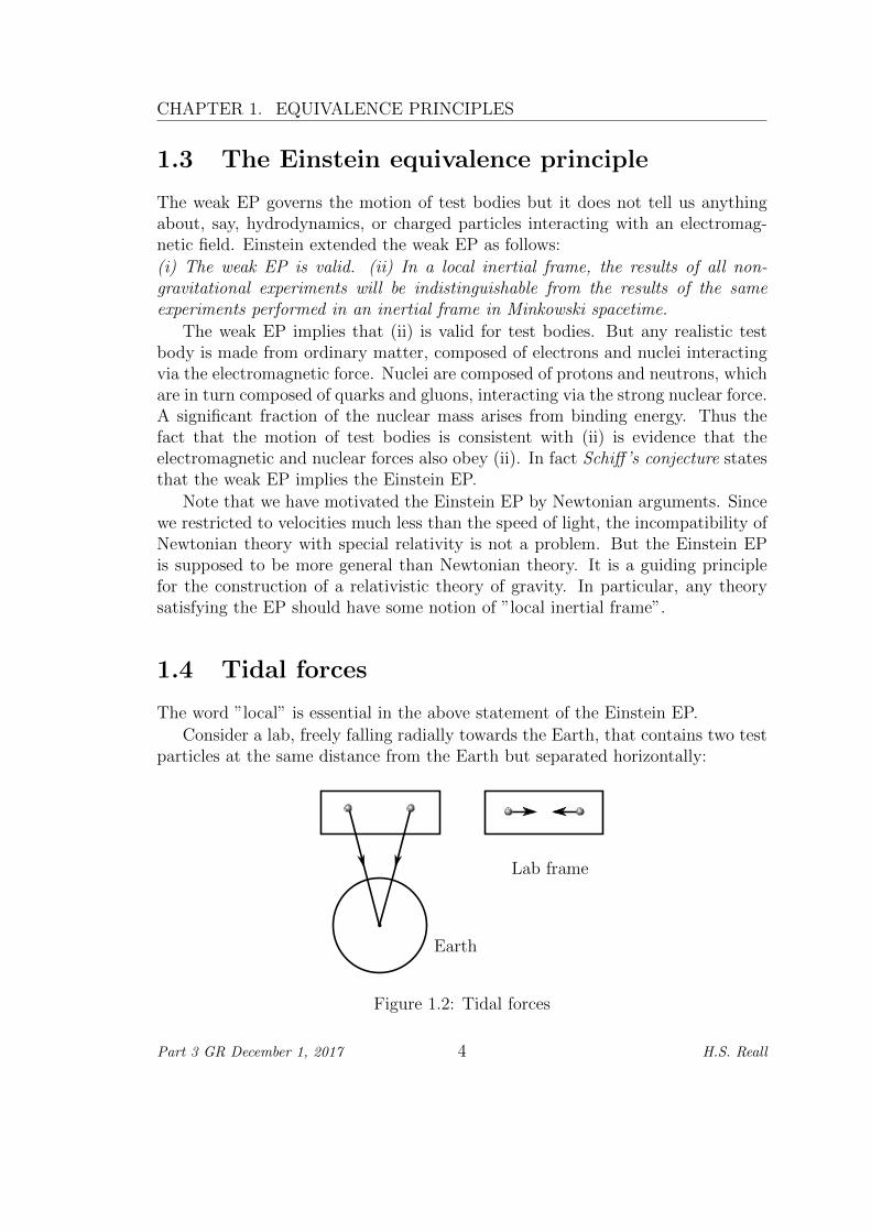
Consider a lab, freely falling radially towards the Earth, that contains two testparticles at the same distance from the Earth but separated horizontally:
Earth
Lab frame
Figure 1.2: Tidal forces
Part 3 GR December 1, 2017 4 H.S. Reall
1.5. BENDING OF LIGHT
The gravitational attraction of the particles is tiny and can be neglected. Nev-ertheless, as the lab falls towards Earth, the particles will accelerate towards eachother because the gravitational field has a slightly different direction at the loca-tion of the two particles. This is an example of a tidal force: a force arising fromnon-uniformity of the gravitational field. Such forces are physical: they cannot beeliminated by free fall.
1.5 Bending of light
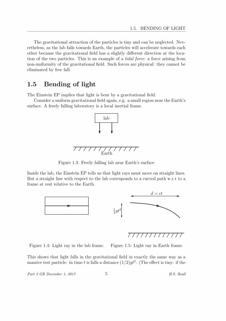
The Einstein EP implies that light is bent by a gravitational field.Consider a uniform gravitational field again, e.g. a small region near the Earth’s
surface. A freely falling laboratory is a local inertial frame.
Earth
lab
Figure 1.3: Freely falling lab near Earth’s surface
Inside the lab, the Einstein EP tells us that light rays must move on straight lines.But a straight line with respect to the lab corresponds to a curved path w.r.t to aframe at rest relative to the Earth.
Figure 1.4: Light ray in the lab frame.
d = ct
12gt2
Figure 1.5: Light ray in Earth frame.
This shows that light falls in the gravitational field in exactly the same way as amassive test particle: in time t is falls a distance (1/2)gt2. (The effect is tiny: if the
Part 3 GR December 1, 2017 5 H.S. Reall
CHAPTER 1. EQUIVALENCE PRINCIPLES
field is vertical then the time taken for the light to travel a horizontal distance dis t = d/c. In this time, the light falls a distance h = gd2/(2c2). Taking d = 1 km,g ≈ 10ms−2 gives h ≈ 5× 10⁻¹¹m.)
NB: this is a local effect in which the gravitational field is approximated asuniform so the result follows from the EP. It can’t be used to calculate the bendingof light rays by a non-uniform gravitational field e.g. light bending by the the Sun.
1.6 Gravitational red shift
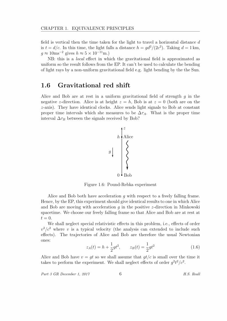
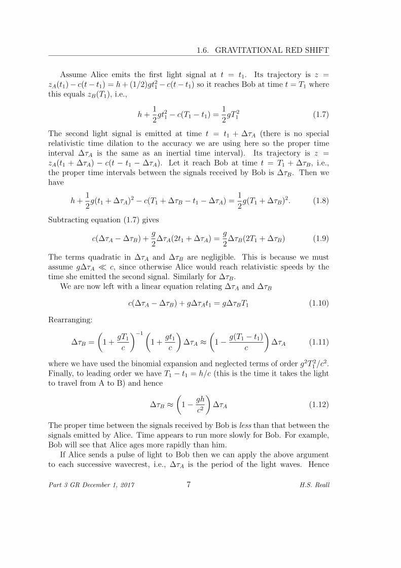
Alice and Bob are at rest in a uniform gravitational field of strength g in thenegative z-direction. Alice is at height z = h, Bob is at z = 0 (both are on thez-axis). They have identical clocks. Alice sends light signals to Bob at constantproper time intervals which she measures to be ∆τA. What is the proper timeinterval ∆τB between the signals received by Bob?
g
Bob
Aliceh
z
0
Figure 1.6: Pound-Rebka experiment
Alice and Bob both have acceleration g with respect to a freely falling frame.Hence, by the EP, this experiment should give identical results to one in which Aliceand Bob are moving with acceleration g in the positive z-direction in Minkowskispacetime. We choose our freely falling frame so that Alice and Bob are at rest att = 0.
We shall neglect special relativistic effects in this problem, i.e., effects of orderv2/c2 where v is a typical velocity (the analysis can extended to include sucheffects). The trajectories of Alice and Bob are therefore the usual Newtonianones:
zA(t) = h+1
2gt2, zB(t) =
1
2gt2 (1.6)
Alice and Bob have v = gt so we shall assume that gt/c is small over the time ittakes to perform the experiment. We shall neglect effects of order g2t2/c2.
Part 3 GR December 1, 2017 6 H.S. Reall
1.6. GRAVITATIONAL RED SHIFT
Assume Alice emits the first light signal at t = t1. Its trajectory is z =zA(t1)− c(t− t1) = h+ (1/2)gt21− c(t− t1) so it reaches Bob at time t = T1 wherethis equals zB(T1), i.e.,
h+1
2gt21 − c(T1 − t1) =
1
2gT 2
1 (1.7)
The second light signal is emitted at time t = t1 + ∆τA (there is no specialrelativistic time dilation to the accuracy we are using here so the proper timeinterval ∆τA is the same as an inertial time interval). Its trajectory is z =zA(t1 + ∆τA) − c(t − t1 − ∆τA). Let it reach Bob at time t = T1 + ∆τB, i.e.,the proper time intervals between the signals received by Bob is ∆τB. Then wehave
h+1
2g(t1 + ∆τA)2 − c(T1 + ∆τB − t1 −∆τA) =
1
2g(T1 + ∆τB)2. (1.8)
Subtracting equation (1.7) gives
c(∆τA −∆τB) +g
2∆τA(2t1 + ∆τA) =
g
2∆τB(2T1 + ∆τB) (1.9)
The terms quadratic in ∆τA and ∆τB are negligible. This is because we mustassume g∆τA c, since otherwise Alice would reach relativistic speeds by thetime she emitted the second signal. Similarly for ∆τB.
We are now left with a linear equation relating ∆τA and ∆τB
c(∆τA −∆τB) + g∆τAt1 = g∆τBT1 (1.10)
Rearranging:
∆τB =
(1 +
gT1
c
)−1(1 +
gt1c
)∆τA ≈
(1− g(T1 − t1)
c
)∆τA (1.11)
where we have used the binomial expansion and neglected terms of order g2T 21 /c
2.Finally, to leading order we have T1 − t1 = h/c (this is the time it takes the lightto travel from A to B) and hence
∆τB ≈(
1− gh
c2
)∆τA (1.12)
The proper time between the signals received by Bob is less than that between thesignals emitted by Alice. Time appears to run more slowly for Bob. For example,Bob will see that Alice ages more rapidly than him.
If Alice sends a pulse of light to Bob then we can apply the above argumentto each successive wavecrest, i.e., ∆τA is the period of the light waves. Hence
Part 3 GR December 1, 2017 7 H.S. Reall
CHAPTER 1. EQUIVALENCE PRINCIPLES
∆τA = λA/c where λA is the wavelength of the light emitted by Alice. Bobreceives light with wavelength λB where ∆τB = λB/c. Hence we have
λB ≈(
1− gh
c2
)λA. (1.13)
The light received by Bob has shorter wavelength than the light emitted by Alice:it has undergone a blueshift. Light falling in a gravitational field is blueshifted.
This prediction of the EP was confirmed experimentally by the Pound-Rebkaexperiment (1960) in which light was emitted at the top of a tower and absorbedat the bottom. High accuracy was needed since gh/c2 = O(10−15).
An identical argument reveals that light climbing out of a gravitational fieldundergoes a redshift. We can write the above formula in a form that applies toboth situations:
∆τB ≈(
1 +ΦB − ΦA
c2
)∆τA (1.14)
where Φ is the gravitational potential. Our derivation of this result, using theEP, is valid only for uniform gravitational fields. However, we will see that GRpredicts that this result is valid also for weak non-uniform fields.
1.7 Curved spacetime
The weak EP states that if two test bodies initially have the same position andvelocity then they will follow exactly the same trajectory in a gravitational field,even if they have very different composition. (This is not true of other forces: in anelectromagnetic field, bodies with different charge to mass ratio will follow differenttrajectories.) This suggested to Einstein that the trajectories of test bodies in agravitational field are determined by the structure of spacetime alone and hencegravity should be described geometrically.
To see the idea, consider a spacetime in which the proper time between twoinfinitesimally nearby events is given not by the Minkowskian formula
c2dτ 2 = c2dt2 − dx2 − dy2 − dz2 (1.15)
but instead by
c2dτ 2 =
(1 +
2Φ(x, y, z)
c2
)c2dt2 −
(1− 2Φ(x, y, z)
c2
)(dx2 + dy2 + dz2), (1.16)
where Φ/c2 1. Let Alice have spatial position xA = (xA, yA, zA) and Bob havespatial position xB. Assume that Alice sends a light signal to Bob at time tA anda second signal at time tA + ∆t. Let Bob receive the first signal at time tB. What
Part 3 GR December 1, 2017 8 H.S. Reall
1.7. CURVED SPACETIME
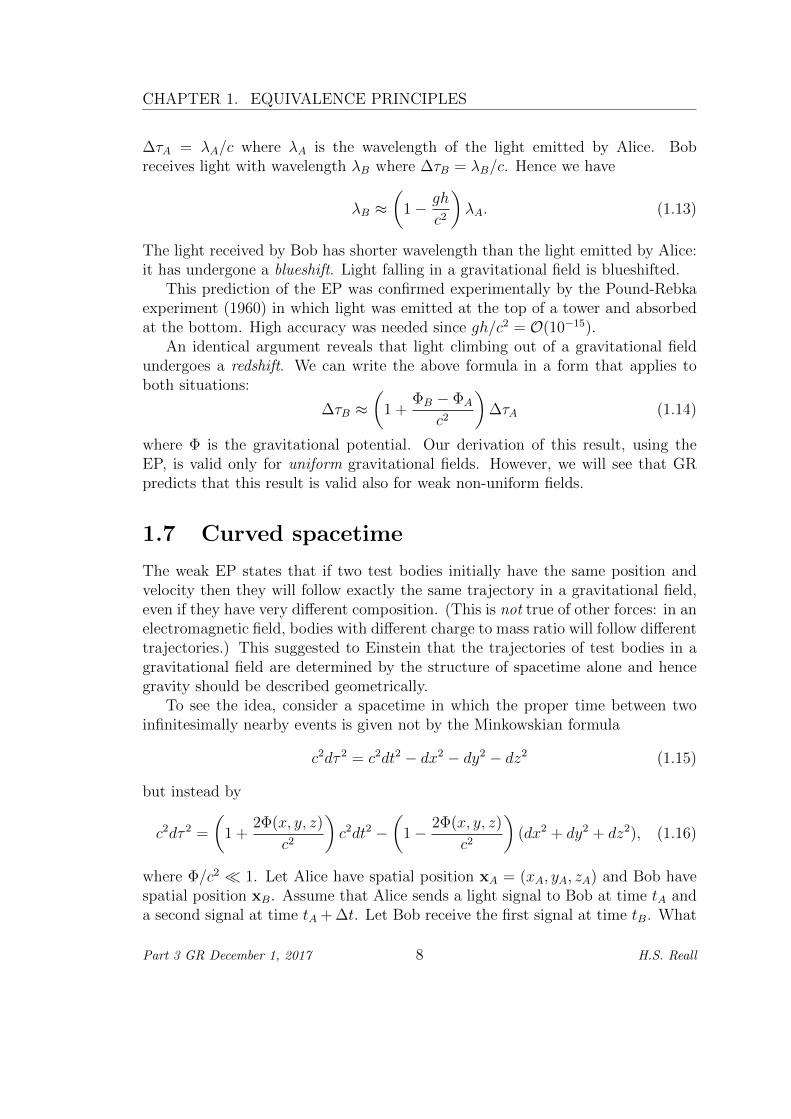
time does he receive the second signal? We haven’t discussed how one determinesthe trajectory of the light ray but this doesn’t matter. The above geometry doesnot depend on t. Hence the trajectory of the second signal must be the same asthe first signal (whatever this is) but simply shifted by a time ∆t:
x
t
A B
tA
tA + ∆t
tB
tB + ∆t
1st phot
on2
ndph
oton
Figure 1.7: Light ray paths
Hence Bob receives the second signal at time tB +∆t. The proper time intervalbetween the signals sent by Alice is given by
∆τ 2A =
(1 +
2ΦA
c2
)∆t2, (1.17)
where ΦA ≡ Φ(xA). (Note ∆x = ∆y = ∆z = 0 because her signals are sent fromthe same spatial position.) Hence, using Φ/c2 1,
∆τA =
(1 +
2ΦA
c2
)1/2
≈(
1 +ΦA
c2
)∆t. (1.18)
Similarly, the proper time between the signals received by Bob is
∆τB ≈(
1 +ΦB
c2
)∆t. (1.19)
Hence, eliminating ∆t:
∆τB ≈(
1 +ΦB
c2
)(1 +
ΦA
c2
)−1
∆τA ≈(
1 +ΦB − ΦA
c2
)∆τA, (1.20)
which is just equation (1.14). The difference in the rates of the two clocks hasbeen explained by the geometry of spacetime. The geometry (1.16) is actuallythe geometry predicted by General Relativity outside a time-independent, non-rotating distribution of matter, at least when gravity is weak, i.e., |Φ|/c2 1.(This is true in the Solar System: |Φ|/c2 = GM/(rc2) ∼ 10−5 at the surface of theSun.)
Part 3 GR December 1, 2017 9 H.S. Reall

CHAPTER 1. EQUIVALENCE PRINCIPLES
Part 3 GR December 1, 2017 10 H.S. Reall
Chapter 2
Manifolds and tensors
2.1 Introduction
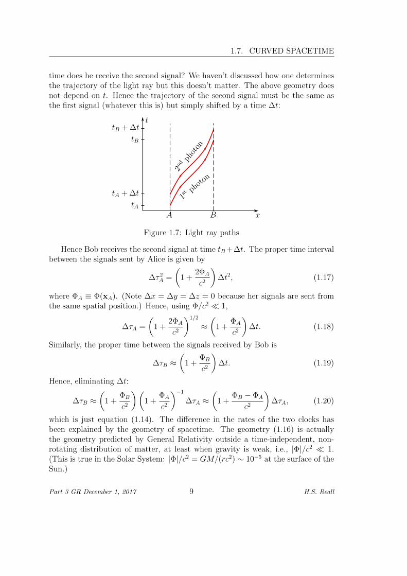
In Minkowski spacetime we usually use inertial frame coordinates (t, x, y, z) sincethese are adapted to the symmetries of the spacetime so using these coordinatessimplifies the form of physical laws. However, a general spacetime has no sym-metries and therefore no preferred set of coordinates. In fact, a single set ofcoordinates might not be sufficient to describe the spacetime. A simple exampleof this is provided by spherical polar coordinates (θ, φ) on the surface of the unitsphere S2 in R3:
x
y
z
φ
θ
Figure 2.1: Spherical polar coordinates
These coordinates are not well-defined at θ = 0, π (what is the value of φthere?). Furthermore, the coordinate φ is discontinuous at φ = 0 or 2π.
To describe S2 so that a pair of coordinates is assigned in a smooth way toevery point, we need to use several overlapping sets of coordinates. Generalizingthis example leads to the idea of a manifold. In GR, we assume that spacetime isa 4-dimensional differentiable manifold.
11
CHAPTER 2. MANIFOLDS AND TENSORS
2.2 Differentiable manifolds
You know how to do calculus on Rn. How do you do calculus on a curved space,e.g., S2? Locally, S2 looks like R2 so one can carry over standard results. However,one has to confront the fact that it is impossible to use a single coordinate systemon S2. In order to do calculus we need our coordinates systems to ”mesh together”in a smooth way. Mathematically, this is captured by the notion of a differentiablemanifold:
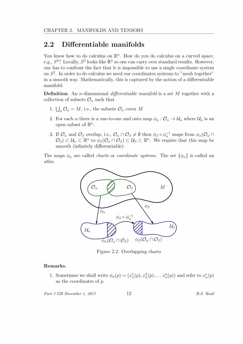
Definition. An n-dimensional differentiable manifold is a set M together with acollection of subsets Oα such that
1.⋃αOα = M , i.e., the subsets Oα cover M
2. For each α there is a one-to-one and onto map φα : Oα → Uα where Uα is anopen subset of Rn.
3. If Oα and Oβ overlap, i.e., Oα ∩ Oβ 6= ∅ then φβ φ−1α maps from φα(Oα ∩
Oβ) ⊂ Uα ⊂ Rn to φβ(Oα ∩ Oβ) ⊂ Uβ ⊂ Rn. We require that this map besmooth (infinitely differentiable).
The maps φα are called charts or coordinate systems. The set φα is called anatlas.
φβφα
Oα Oβ M
UαUβ
φβ φ−1α
φα(Oα ∩ Oβ) φβ(Oα ∩ Oβ)
Figure 2.2: Overlapping charts
Remarks.
1. Sometimes we shall write φα(p) = (x1α(p), x2
α(p), . . . xnα(p)) and refer to xiα(p)as the coordinates of p.
Part 3 GR December 1, 2017 12 H.S. Reall
2.2. DIFFERENTIABLE MANIFOLDS
2. Strictly speaking, we have defined above the notion of a smooth manifold. Ifwe replace ”smooth” in the definition by Ck (k-times continuously differen-tiable) then we obtain a Ck-manifold. We shall always assume the manifoldis smooth.
Examples.
1. Rn: this is a manifold with atlas consisting of the single chart φ : (x1, . . . , xn) 7→(x1, . . . , xn).
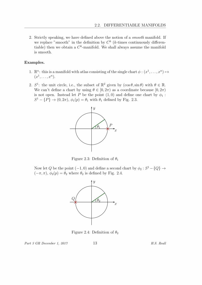
2. S1: the unit circle, i.e., the subset of R2 given by (cos θ, sin θ) with θ ∈ R.We can’t define a chart by using θ ∈ [0, 2π) as a coordinate because [0, 2π)is not open. Instead let P be the point (1, 0) and define one chart by φ1 :S1 − P → (0, 2π), φ1(p) = θ1 with θ1 defined by Fig. 2.3.
x
y
θ1P
Figure 2.3: Definition of θ1
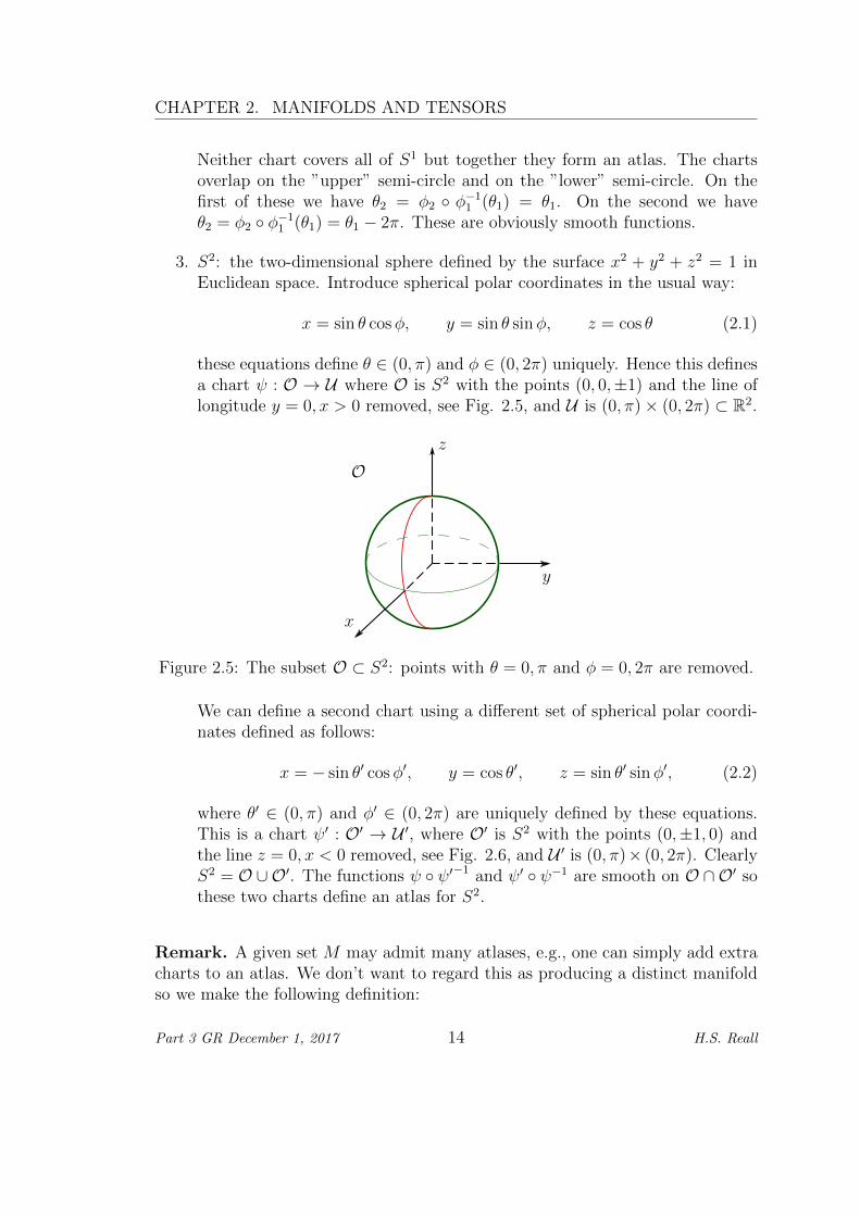
Now let Q be the point (−1, 0) and define a second chart by φ2 : S1−Q →(−π, π), φ2(p) = θ2 where θ2 is defined by Fig. 2.4.
x
y
θ2Q
Figure 2.4: Definition of θ2
Part 3 GR December 1, 2017 13 H.S. Reall
CHAPTER 2. MANIFOLDS AND TENSORS
Neither chart covers all of S1 but together they form an atlas. The chartsoverlap on the ”upper” semi-circle and on the ”lower” semi-circle. On thefirst of these we have θ2 = φ2 φ−1
1 (θ1) = θ1. On the second we haveθ2 = φ2 φ−1
1 (θ1) = θ1 − 2π. These are obviously smooth functions.
3. S2: the two-dimensional sphere defined by the surface x2 + y2 + z2 = 1 inEuclidean space. Introduce spherical polar coordinates in the usual way:
x = sin θ cosφ, y = sin θ sinφ, z = cos θ (2.1)
these equations define θ ∈ (0, π) and φ ∈ (0, 2π) uniquely. Hence this definesa chart ψ : O → U where O is S2 with the points (0, 0,±1) and the line oflongitude y = 0, x > 0 removed, see Fig. 2.5, and U is (0, π)× (0, 2π) ⊂ R2.
x
y
z
O
Figure 2.5: The subset O ⊂ S2: points with θ = 0, π and φ = 0, 2π are removed.
We can define a second chart using a different set of spherical polar coordi-nates defined as follows:
x = − sin θ′ cosφ′, y = cos θ′, z = sin θ′ sinφ′, (2.2)
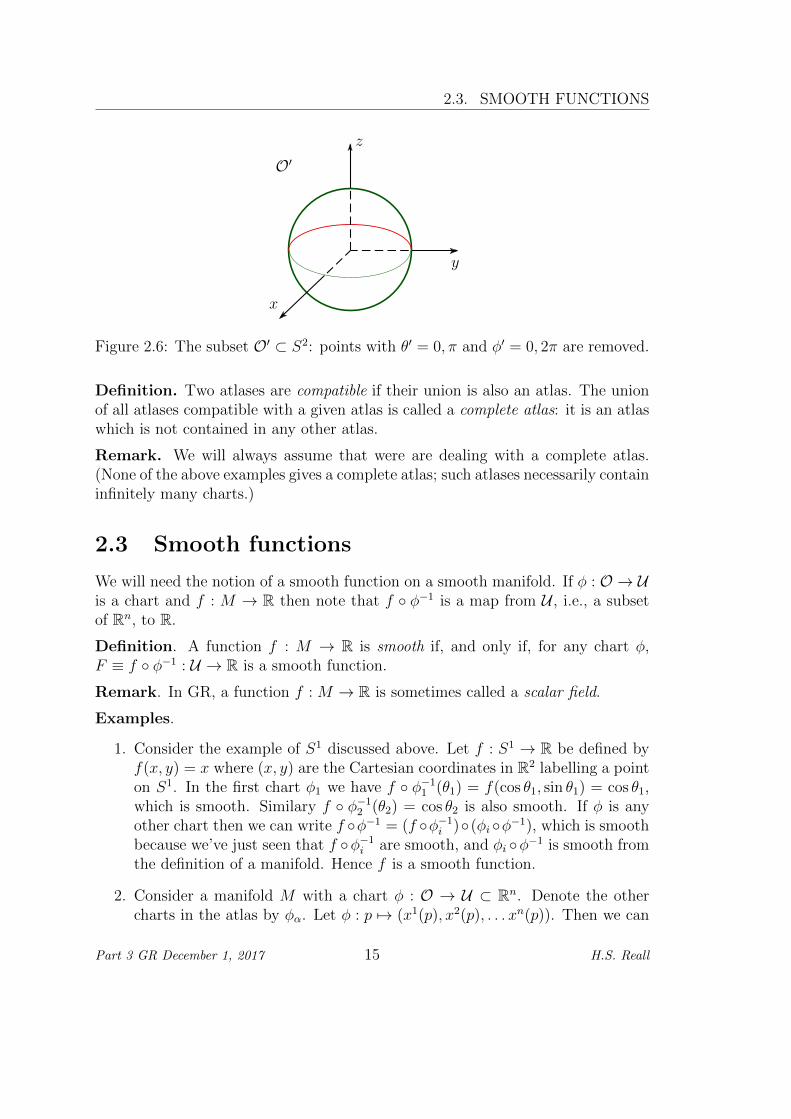
where θ′ ∈ (0, π) and φ′ ∈ (0, 2π) are uniquely defined by these equations.This is a chart ψ′ : O′ → U ′, where O′ is S2 with the points (0,±1, 0) andthe line z = 0, x < 0 removed, see Fig. 2.6, and U ′ is (0, π)× (0, 2π). ClearlyS2 = O ∪O′. The functions ψ ψ′−1 and ψ′ ψ−1 are smooth on O ∩O′ sothese two charts define an atlas for S2.
Remark. A given set M may admit many atlases, e.g., one can simply add extracharts to an atlas. We don’t want to regard this as producing a distinct manifoldso we make the following definition:
Part 3 GR December 1, 2017 14 H.S. Reall
2.3. SMOOTH FUNCTIONS
x
y
z
O′
Figure 2.6: The subset O′ ⊂ S2: points with θ′ = 0, π and φ′ = 0, 2π are removed.
Definition. Two atlases are compatible if their union is also an atlas. The unionof all atlases compatible with a given atlas is called a complete atlas: it is an atlaswhich is not contained in any other atlas.
Remark. We will always assume that were are dealing with a complete atlas.(None of the above examples gives a complete atlas; such atlases necessarily containinfinitely many charts.)
2.3 Smooth functions
We will need the notion of a smooth function on a smooth manifold. If φ : O → Uis a chart and f : M → R then note that f φ−1 is a map from U , i.e., a subsetof Rn, to R.
Definition. A function f : M → R is smooth if, and only if, for any chart φ,F ≡ f φ−1 : U → R is a smooth function.
Remark. In GR, a function f : M → R is sometimes called a scalar field.
Examples.
1. Consider the example of S1 discussed above. Let f : S1 → R be defined byf(x, y) = x where (x, y) are the Cartesian coordinates in R2 labelling a pointon S1. In the first chart φ1 we have f φ−1
1 (θ1) = f(cos θ1, sin θ1) = cos θ1,which is smooth. Similary f φ−1
2 (θ2) = cos θ2 is also smooth. If φ is anyother chart then we can write f φ−1 = (f φ−1
i )(φiφ−1), which is smoothbecause we’ve just seen that f φ−1
i are smooth, and φi φ−1 is smooth fromthe definition of a manifold. Hence f is a smooth function.
2. Consider a manifold M with a chart φ : O → U ⊂ Rn. Denote the othercharts in the atlas by φα. Let φ : p 7→ (x1(p), x2(p), . . . xn(p)). Then we can
Part 3 GR December 1, 2017 15 H.S. Reall
CHAPTER 2. MANIFOLDS AND TENSORS
regard x1 (say) as a function on the subset O of M . Is it a smooth function?Yes: x1 φ−1
α is smooth for any chart φα, because it is the first componentof the map φ φ−1
α , and the latter is smooth by the definition of a manifold.
3. Often it is convenient to define a function by specifying F instead of f .More precisely, given an atlas φα, we define f by specifying functionsFα : Uα → R and then setting f = Fα φα. One has to make sure that theresulting definition is independent of α on chart overlaps. For example, forS1 using the atlas discussed above, define F1 : (0, 2π)→ R by θ1 7→ sin(mθ1)and F2 : (−π, π)→ R by θ2 7→ sin(mθ2), where m is an integer. On the chartoverlaps we have F1 φ1 = F2 φ2 because θ1 and θ2 differ by a multiple of2π on both overlaps. Hence this defines a function on S1.
Remark. After a while we will stop distinguishing between f and F , i.e., we willsay f(x) when we mean F (x).
2.4 Curves and vectors
Rn, or Minkowski spacetime, has the structure of a vector space, e.g., it makessense to add the position vectors of points. One can view more general vectors,e.g., the 4-velocity of a particle, as vectors in the space itself. This structure doesnot extend to more general manifolds, e.g., S2. So we need to discuss how to definevectors on manifolds.
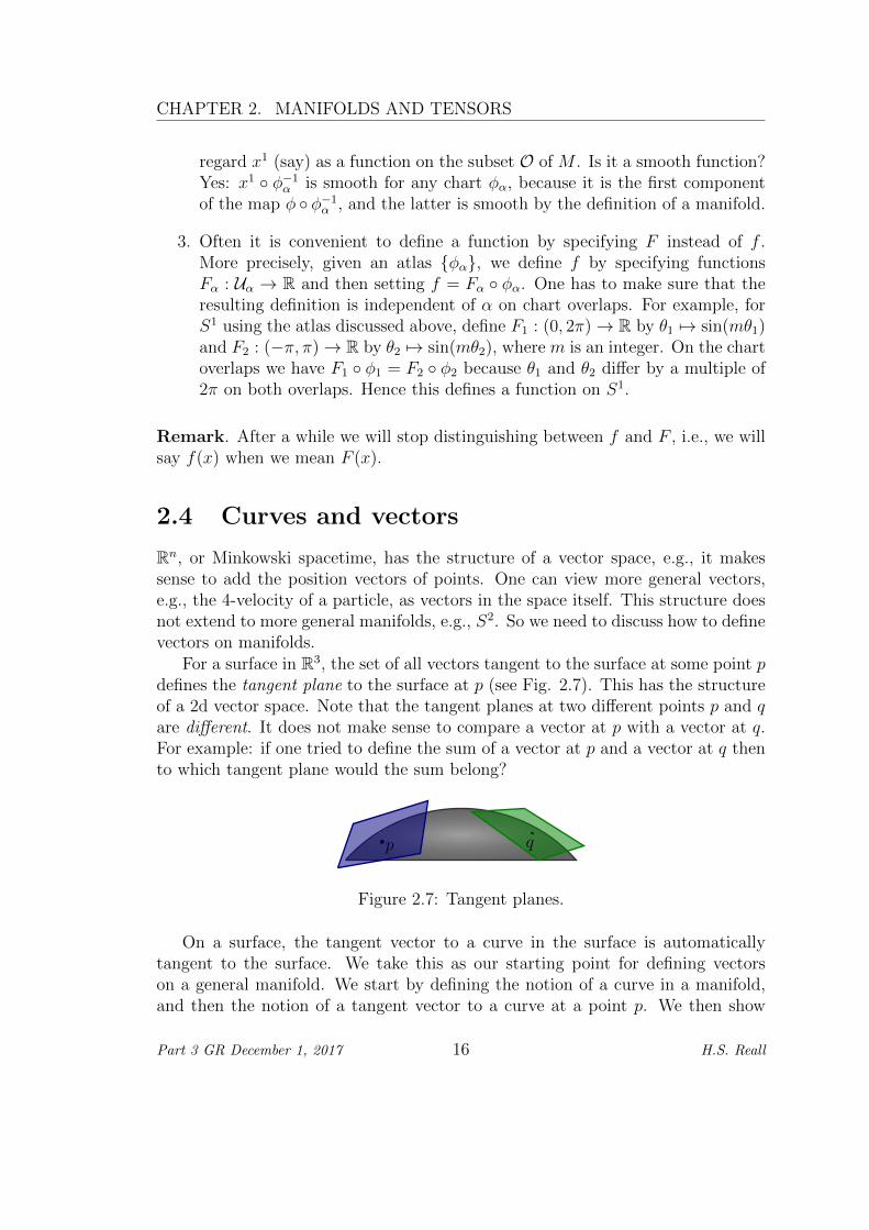
For a surface in R3, the set of all vectors tangent to the surface at some point pdefines the tangent plane to the surface at p (see Fig. 2.7). This has the structureof a 2d vector space. Note that the tangent planes at two different points p and qare different. It does not make sense to compare a vector at p with a vector at q.For example: if one tried to define the sum of a vector at p and a vector at q thento which tangent plane would the sum belong?
p q
Figure 2.7: Tangent planes.
On a surface, the tangent vector to a curve in the surface is automaticallytangent to the surface. We take this as our starting point for defining vectorson a general manifold. We start by defining the notion of a curve in a manifold,and then the notion of a tangent vector to a curve at a point p. We then show
Part 3 GR December 1, 2017 16 H.S. Reall
2.4. CURVES AND VECTORS
that the set of all such tangent vectors at p forms a vector space Tp(M). This isthe analogue of the tangent plane to a surface but it makes no reference to anyembedding into a higher-dimensional space.
Definition A smooth curve in a differentiable manifold M is a smooth functionλ : I → M , where I is an open interval in R (e.g. (0, 1) or (−1,∞)). By this wemean that φα λ is a smooth map from I to Rn for all charts φα.
Let f : M → R and λ : I → M be a smooth function and a smooth curverespectively. Then f λ is a map from I to R. Hence we can take its derivativeto obtain the rate of change of f along the curve:
d
dt[(f λ)(t)] =
d
dt[f(λ(t))] (2.3)
In Rn we are used to the idea that the rate of change of f along the curve at apoint p is given by the directional derivative Xp · (∇f)p where Xp is the tangentto the curve at p. Note that the vector Xp defines a linear map from the space ofsmooth functions on Rn to R: f 7→ Xp · (∇f)p. This is how we define a tangentvector to a curve in a general manifold:
Definition. Let λ : I →M be a smooth curve with (wlog) λ(0) = p. The tangentvector to λ at p is the linear map Xp from the space of smooth functions on M toR defined by
Xp(f) =
d
dt[f(λ(t))]
t=0
(2.4)
Note that this satisfies two important properties: (i) it is linear, i.e., Xp(f + g) =Xp(f)+Xp(g) and Xp(αf) = αXp(f) for any constant α; (ii) it satisfies the Leibnizrule Xp(fg) = Xp(f)g(p) + f(p)Xp(g), where f and g are smooth functions andfg is their product.
If φ = (x1, x2, . . . xn) is a chart defined in a neighbourhood of p and F ≡ f φ−1
then we have f λ = f φ−1 φ λ = F φ λ and hence
Xp(f) =
(∂F (x)
∂xµ
)φ(p)
(dxµ(λ(t))
dt
)t=0
(2.5)
Note that (i) the first term on the RHS depends only on f and φ, and the secondterm on the RHS depends only on φ and λ; (ii) we are using the Einstein summationconvention, i.e., µ is summed from 1 to n in the above expression.
Proposition. The set of all tangent vectors at p forms a n-dimensional vectorspace, the tangent space Tp(M).Proof. Consider curves λ and κ through p, wlog λ(0) = κ(0) = p. Let theirtangent vectors at p be Xp and Yp respectively. We need to define addition of
Part 3 GR December 1, 2017 17 H.S. Reall
CHAPTER 2. MANIFOLDS AND TENSORS
tangent vectors and multiplication by a constant. let α and β be constants. Wedefine αXp + βYp to be the linear map f 7→ αXp(f) + βYp(f). Next we needto show that this linear map is indeed the tangent vector to a curve through p.Let φ = (x1, . . . , xn) be a chart defined in a neighbourhood of p. Consider thefollowing curve:
ν(t) = φ−1 [α(φ(λ(t))− φ(p)) + β(φ(κ(t))− φ(p)) + φ(p)] (2.6)
Note that ν(0) = p. Let Zp denote the tangent vector to this curve at p. Fromequation (2.5) we have
Zp(f) =
(∂F (x)
∂xµ
)φ(p)
d
dt[α(xµ(λ(t))− xµ(p)) + β(xµ(κ(t))− xµ(p)) + xµ(p)]
t=0
=
(∂F (x)
∂xµ
)φ(p)
[α
(dxµ(λ(t))
dt
)t=0
+ β
(dxµ(κ(t))
dt
)t=0
]= αXp(f) + βYp(f)
= (αXp + βYp)(f).
Since this is true for any smooth function f , we have Zp = αXp +βYp as required.Hence αXp + βYp is tangent to the curve ν at p. It follows that the set of tangentvectors at p forms a vector space (the zero vector is realized by the curve λ(t) = pfor all t).
The next step is to show that this vector space is n-dimensional. To do this,we exhibit a basis. Let 1 ≤ µ ≤ n. Consider the curve λµ through p defined by
λµ(t) = φ−1(x1(p), . . . , xµ−1(p), xµ(p) + t, xµ+1(p), . . . , xn(p)). (2.7)
The tangent vector to this curve at p is denoted(
∂∂xµ
)p. To see why, note that,
using equation (2.5) (∂
∂xµ
)p
(f) =
(∂F
∂xµ
)φ(p)
. (2.8)
The n tangent vectors(
∂∂xµ
)p
are linearly independent. To see why, assume that
there exist constants αµ such that αµ(
∂∂xµ
)p
= 0. Then, for any function f we
must have
αµ(∂F (x)
∂xµ
)φ(p)
= 0. (2.9)
Choosing F = xν , this reduces to αν = 0. Letting this run over all values of ν wesee that all of the constants αν must vanish, which proves linear independence.
Part 3 GR December 1, 2017 18 H.S. Reall
2.4. CURVES AND VECTORS
Finally we must prove that these tangent vectors span the vector space. Thisfollows from equation (2.5), which can be rewritten
Xp(f) =
(dxµ(λ(t))
dt
)t=0
(∂
∂xµ
)p
(f) (2.10)
this is true for any f hence
Xp =
(dxµ(λ(t))
dt
)t=0
(∂
∂xµ
)p
, (2.11)
i.e. Xp can be written as a linear combination of the n tangent vectors(
∂∂xµ
)p.
These n vectors therefore form a basis for Tp(M), which establishes that the tan-gent space is n-dimensional. QED.
Remark. The basis (
∂∂xµ
)p, µ = 1, . . . n is chart-dependent: we had to choose
a chart φ defined in a neighbourhood of p to define it. Choosing a different chartwould give a different basis for Tp(M). A basis defined this way is sometimes calleda coordinate basis.
Definition. Let eµ, µ = 1 . . . n be a basis for Tp(M) (not necessarily a coordinatebasis). We can expand any vector X ∈ Tp(M) as X = Xµeµ. We call the numbersXµ the components of X with respect to this basis.
Example. Using the coordinate basis eµ = (∂/∂xµ)p, equation (2.11) shows thatthe tangent vector Xp to a curve λ(t) at p (where t = 0) has components
Xµp =
(dxµ(λ(t))
dt
)t=0
. (2.12)
Remark. Note the placement of indices. We shall sum over repeated indicesif one such index appears ”upstairs” (as a superscript, e.g., Xµ) and the other”downstairs” (as a subscript, e.g., eµ). (The index µ on
(∂∂xµ
)p
is regarded as
downstairs.) If an equation involves the same index more than twice, or twice butboth times upstairs or both times downstairs (e.g. XµYµ) then a mistake has beenmade.
Let’s consider the relationship between different coordinate bases. Let φ = (x1, . . . , xn)and φ′ = (x′1, . . . , x′n) be two charts defined in a neighbourhood of p. Then, forany smooth function f , we have(
∂
∂xµ
)p
(f) =
(∂
∂xµ(f φ−1)
)φ(p)
=
(∂
∂xµ[(f φ′−1
) (φ′ φ−1)]
)φ(p)
Part 3 GR December 1, 2017 19 H.S. Reall
CHAPTER 2. MANIFOLDS AND TENSORS
Now let F ′ = f φ′−1. This is a function of the coordinates x′. Note that thecomponents of φ′φ−1 are simply the functions x′µ(x), i.e., the primed coordinatesexpressed in terms of the unprimed coordinates. Hence what we have is easy toevaluate using the chain rule:(
∂
∂xµ
)p
(f) =
(∂
∂xµ(F ′(x′(x)))
)φ(p)
=
(∂x′ν
∂xµ
)φ(p)
(∂F ′(x′)
∂x′ν
)φ′(p)
=
(∂x′ν
∂xµ
)φ(p)
(∂
∂x′ν
)p
(f)
Hence we have (∂
∂xµ
)p
=
(∂x′ν
∂xµ
)φ(p)
(∂
∂x′ν
)p
(2.13)
This expresses one set of basis vectors in terms of the other. Let Xµ and X ′µ
denote the components of a vector with respect to the two bases. Then we have
X = Xν
(∂
∂xν
)p
= Xν
(∂x′µ
∂xν
)φ(p)
(∂
∂x′µ
)p
(2.14)
and hence
X ′µ
= Xν
(∂x′µ
∂xν
)φ(p)
(2.15)
Elementary treatments of GR usually define a vector to be a set of numbers Xµthat transforms according to this rule under a change of coordinates. More pre-cisely, they usually call this a ”contravariant vector”.
2.5 Covectors
Recall the following from linear algebra:
Definition. Let V be a real vector space. The dual space V ∗ of V is the vectorspace of linear maps from V to R.
Lemma. If V is n-dimensional then so is V ∗. If eµ, µ = 1, . . . , n is a basis forV then V ∗ has a basis fµ, µ = 1, . . . , n, the dual basis defined by fµ(eν) = δµν(if X = Xµeµ then fµ(X) = Xνfµ(eν) = Xµ).
Since V and V ∗ have the same dimension, they are isomorphic. For example thelinear map defined by eµ 7→ fµ is an isomorphism. But this is basis-dependent: a
Part 3 GR December 1, 2017 20 H.S. Reall
2.5. COVECTORS
different choice of basis would give a different isomorphism. In contrast, there isa natural (basis-independent) isomorphism between V and (V ∗)∗:
Theorem. If V is finite dimensional then (V ∗)∗ is naturally isomorphic to V . Theisomorphism is Φ : V → (V ∗)∗ where Φ(X)(ω) = ω(X) for all ω ∈ V ∗.
Now we return to manifolds:
Definition. The dual space of Tp(M) is denoted T ∗p (M) and called the cotangentspace at p. An element of this space is called a covector (or 1-form) at p. If eµis a basis for Tp(M) and fµ is the dual basis then we can expand a covector ηas ηµf
µ. ηµ are called the components of η.
Note that (i) η(eµ) = ηνfν(eµ) = ηµ; (ii) if X ∈ Tp(M) then η(X) = η(Xµeµ) =
Xµη(eµ) = Xµηµ (note the placement of indices!)
Definition. Let f : M → R be a smooth function. Define a covector (df)p by(df)p(X) = X(f) for any vector X ∈ Tp(M). (df)p is the gradient of f at p.
Examples.
1. Let (x1, . . . , xn) be a coordinate chart defined in a neighbourhood of p, recallthat xµ is a smooth function (in this neighbourhood) so we can take f = xµ
in the above definition to define n covectors (dxµ)p. Note that
(dxµ)p
((∂
∂xν
)p
)=
(∂xµ
∂xν
)p
= δµν (2.16)
Hence (dxµ)p is the dual basis of (∂/∂xµ)p.
2. To explain why we call (df)p the gradient of f at p, observe that its compo-nents in a coordinate basis are
[(df)p]µ = (df)p
((∂
∂xµ
)p
)=
(∂
∂xµ
)p
(f) =
(∂F
∂xµ
)φ(p)
(2.17)
where the first equality uses (i) above, the second equality is the definitionof (df)p and the final equality used (2.8).
Exercise. Consider two different charts φ = (x1, . . . , xn) and φ′ = (x′1, . . . , x′n)defined in a neighbourhood of p. Show that
(dxµ)p =
(∂xµ
∂x′ν
)φ′(p)
(dx′ν)p, (2.18)
Part 3 GR December 1, 2017 21 H.S. Reall
CHAPTER 2. MANIFOLDS AND TENSORS
and hence that, if ωµ and ω′µ are the components of ω ∈ T ∗p (M) w.r.t. the twocoordinate bases, then
ω′µ =
(∂xν
∂x′µ
)φ′(p)
ων . (2.19)
Elementary treatements of GR take this as the definition of a covector, which theyusually call a ”covariant vector”.
2.6 Abstract index notation
So far, we have used Greek letters µ, ν, . . . to denote components of vectors orcovectors with respect to a basis, and also to label the basis vectors themselves(e.g. eµ). Equations involving such indices are assumed to hold only in that basis.For example an equation of the form Xµ = δµ1 says that, in a particular basis,a vector X has only a single non-vanishing component. This will not be true inother bases. Furthermore, if we were just presented with this equation, we wouldnot even know whether or not the quantities Xµ are the components of a vectoror just a set of n numbers.
The abstract index notation uses Latin letters a, b, c, . . .. A vector X is denotedXa or Xb or Xc etc. The letter used in the superscript does not matter. Whatmatters is that there is a superscript Latin letter. This tells us that the objectin question is a vector. We emphasize: Xa represents the vector itself, not acomponent of the vector. Similarly we denote a covector η by ηa (or ηb etc).
If we have an equation involving abstract indices then we can obtain an equationvalid in any particular basis simply by replacing the abstract indices by basisindices (e.g. a → µ, b → ν etc.). For example, consider the quantity ηaX
a in theabstract index notation. We see that this involves a covector ηa and a vector Xa.Furthermore, in any basis, this quantity is equal to ηµX
µ = η(X). Hence ηaXa is
the abstract index way of writing η(X). Similarly, if f is a smooth function thenX(f) = Xa(df)a.
Conversely, if one has an equation involving Greek indices but one knows thatit is true for an arbitrary basis then one can replace the Greek indices with Latinletters.
Latin indices must respect the rules of the summation convention so equationsof the form ηaηa = 1 or ηb = 2 do not make sense.
2.7 Tensors
In Newtonian physics, you are familiar with the idea that certain physical quanti-ties are described by tensors (e.g. the inertia tensor). You may have encountered
Part 3 GR December 1, 2017 22 H.S. Reall
2.7. TENSORS
the idea that the Maxwell field in special relativity is described by a tensor. Ten-sors are very important in GR because the curvature of spacetime is describedwith tensors. In this section we shall define tensors at a point p and explain someof their basic properties.
Definition. A tensor of type (r, s) at p is a multilinear map
T : T ∗p (M)× . . .× T ∗p (M)× Tp(M)× . . .× Tp(M)→ R. (2.20)
where there are r factors of T ∗p (M) and s factors of Tp(M). (Multilinear meansthat the map is linear in each argument.)
In other words, given r covectors and s vectors, a tensor of type (r, s) produces areal number.
Examples.
1. A tensor of type (0, 1) is a linear map Tp(M)→ R, i.e., it is a covector.
2. A tensor of type (1, 0) is a linear map T ∗p (M) → R, i.e., it is an element of(T ∗p (M))∗ but this is naturally isomorphic to Tp(M) hence a tensor of type(1, 0) is a vector. To see how this works, given a vector X ∈ Tp(M) we definea linear map T ∗p (M)→ R by η 7→ η(X) for any η ∈ T ∗p (M).
3. We can define a (1, 1) tensor δ by δ(ω,X) = ω(X) for any covector ω andvector X.
Definition. Let T be a tensor of type (r, s) at p. If eµ is a basis for Tp(M) withdual basis fµ then the components of T in this basis are the numbers
T µ1µ2...µrν1ν2...νs = T (fµ1 , fµ2 , . . . , fµr , eν1 , eν2 , . . . , eνs) (2.21)
In the abstract index notation, we denote T by T a1a2...ar b1b2...bs .
Remark. Tensors of type (r, s) at p can be added together and multiplied by aconstant, hence they form a vector space. Since such a tensor has nr+s components,it is clear that this vector space has dimension nr+s.
Examples.
1. Consider the tensor δ defined above. Its components are
δµν = δ(fµ, eν) = fµ(eν) = δµν , (2.22)
where the RHS is a Kronecker delta. This is true in any basis, so in theabstract index notation we write δ as δab .
Part 3 GR December 1, 2017 23 H.S. Reall
CHAPTER 2. MANIFOLDS AND TENSORS
2. Consider a (2, 1) tensor. Let η and ω be covectors and X a vector. Then inour basis we have
T (η, ω,X) = T (ηµfµ, ωνf
ν , Xρeρ) = ηµωνXρT (fµ, f ν , eρ) = T µνρηµωνX
ρ
(2.23)Now the basis we chose was arbitrary, hence we can immediately convert thisto a basis-independent equation using the abstract index notation:
T (η, ω,X) = T abcηaωbXc. (2.24)
This formula generalizes in the obvious way to a (r, s) tensor.
We have discussed the transformation of vectors and covectors components undera change of coordinate basis. Let’s now examine how tensor components transformunder an arbitrary change of basis. Let eµ and e′µ be two bases for Tp(M).Let fµ and f ′µ denote the corresponding dual bases. Expanding the primedbases in terms of the unprimed bases gives
f ′µ
= Aµνfν , e′µ = Bν
µeν (2.25)
for some matrices Aµν and Bνµ. These matrices are related because:
δµν = f ′µ(e′ν) = Aµρf
ρ(Bσνeσ) = AµρB
σνf
ρ(eσ) = AµρBσνδρσ = AµρB
ρν . (2.26)
Hence Bµν = (A−1)µν . For a change between coordinate bases, our previous results
give
Aµν =
(∂x′µ
∂xν
), Bµ
ν =
(∂xµ
∂x′ν
)(2.27)
and these matrices are indeed inverses of each other (from the chain rule).
Exercise. Show that under an arbitrary change of basis, the components of avector X and a covector η transform as
X ′µ
= AµνXν , η′µ = (A−1)νµην . (2.28)
Show that the components of a (2, 1) tensor T transform as
T ′µνρ = AµσA
ντ (A
−1)λρTστλ. (2.29)
The corresponding result for a (r, s) tensor is an obvious generalization of thisformula.
Given a (r, s) tensor, we can construct a (r− 1, s− 1) tensor by contraction. Thisis easiest to demonstrate with an example.
Part 3 GR December 1, 2017 24 H.S. Reall

2.7. TENSORS
Example. Let T be a tensor of type (3, 2). Define a new tensor S of type (2, 1)as follows
S(ω, η,X) = T (fµ, ω, η, eµ, X) (2.30)
where eµ is a basis and fµ is the dual basis, ω and η are arbitrary covectorsand X is an arbitrary vector. This definition is basis-independent because
T (f ′µ, ω, η, e′µ, X) = T (Aµνf
ν , ω, η, (A−1)ρµeρ, X)
= (A−1)ρµAµνT (f ν , ω, η, eρ, X)
= T (fµ, ω, η, eµ, X).
The components of S and T are related by Sµνρ = T σµνσρ in any basis. Since thisis true in any basis, we can write it using the abstract index notation as
Sabc = T dabdc (2.31)
Note that there are other (2, 1) tensors that we can build from T abcde. For ex-ample, there is T abdcd, which corresponds to replacing the RHS of (2.30) withT (ω, η, fµ, X, eµ). The abstract index notation makes it clear how many differenttensors can be defined this way: we can define a new tensor by ”contracting” anyupstairs index with any downstairs index.
Another important way of constructing new tensors is by taking the product oftwo tensors:
Definition. If S is a tensor of type (p, q) and T is a tensor of type (r, s) then theouter product of S and T , denoted S ⊗ T is a tensor of type (p+ r, q + s) definedby
(S ⊗ T )(ω1, . . . , ωp, η1, . . . , ηr, X1, . . . , Xq, Y1, . . . , Ys)
= S(ω1, . . . , ωp, X1, . . . , Xq)T (η1, . . . , ηr, Y1, . . . , Ys) (2.32)
where ω1, . . . , ωp and η1, . . . , ηr are arbitrary covectors andX1, . . . , Xq and Y1, . . . , Ysare arbitrary vectors.
Exercise. Show that this definition is equivalent to
(S ⊗ T )a1...apb1...br c1...cqd1...ds = Sa1...apc1...cqTb1...br
d1...ds (2.33)
Exercise. Show that, in a coordinate basis, any (2, 1) tensor T at p can be writtenas
T = T µνρ
(∂
∂xµ
)p
⊗(
∂
∂xν
)p
⊗ (dxρ)p (2.34)
This generalizes in the obvious way to a (r, s) tensor.
Part 3 GR December 1, 2017 25 H.S. Reall
CHAPTER 2. MANIFOLDS AND TENSORS
Remark. You may be wondering why we write T abc instead of T abc . At themoment there is no reason why we should not adopt the latter notation. However,it is convenient to generalize our definition of tensors slightly. We have defined a(r, s) tensor to be a linear map with r+ s arguments, where the first r argumentsare covectors and the final s arguments are vectors. We can generalize this byallowing the covectors and vectors to appear in any order. For example, considera (1, 1) tensor. This is a map T ∗p (M) × Tp(M) → R. But we could just as wellhave defined it to be a map Tp(M) × T ∗p (M) → R. The abstract index notationallows us to distinguish these possibilities easily: the first would be written as T aband the second as Ta
b. (2, 1) tensors come in 3 different types: T abc, Tabc and
Tabc. Each type of of (r, s) tensor gives a vector space of dimension nr+s but these
vector spaces are naturally isomorphic so often one does not bother to distinguishbetween them.
There is a final type of tensor operation that we shall need: symmetrizationand antisymmetrization. Consider a (0, 2) tensor T . We can define two other (0, 2)tensors S and A as follows:
S(X, Y ) =1
2(T (X, Y ) + T (Y,X)), A(X, Y ) =
1
2(T (X, Y )− T (Y,X)), (2.35)
where X and Y are vectors at p. In abstract index notation:
Sab =1
2(Tab + Tba), Aab =
1
2(Tab − Tba). (2.36)
In a basis, we can regard the components of T as a square matrix. The componentsof S and A are just the symmetric and antisymmetric parts of this matrix. It isconvenient to introduce some notation to describe the operations we have justdefined: we write
T(ab) =1
2(Tab + Tba), T[ab] =
1
2(Tab − Tba). (2.37)
These operations can be applied to more general tensors. For example,
T (ab)cd =
1
2(T abcd + T bacd). (2.38)
We can also symmetrize or antisymmetrize on more than 2 indices. To symmetrizeon n indices, we sum over all permutations of these indices and divide the resultby n! (the number of permutations). To antisymmetrize we do the same but weweight each term in the sum by the sign of the permutation. The indices that wesymmetrize over must be either upstairs or downstairs, they cannot be a mixture.For example,
T (abc)d =1
3!
(T abcd + T bcad + T cabd + T bacd + T cbad + T acbd
). (2.39)
Part 3 GR December 1, 2017 26 H.S. Reall
2.8. TENSOR FIELDS
T a[bcd] =1
3!(T abcd + T acdb + T adbc − T acbd − T adcb − T abdc) . (2.40)
Sometimes we might wish to (anti)symmetrize over indices which are not ad-jacent. In this case, we use vertical bars to denote indices excluded from the(anti)symmetrization. For example,
T(a|bc|d) =1
2(Tabcd + Tdbca) . (2.41)
Exercise. Show that T (ab)X[a|cd|b] = 0.
2.8 Tensor fields
So far, we have defined vectors, covectors and tensors at a single point p. However,in physics we shall need to consider how these objects vary in spacetime. This leadsus to define vector, covector and tensor fields.
Definition. A vector field is a map X which maps any point p ∈ M to a vectorXp at p. Given a vector field X and a function f we can define a new functionX(f) : M → R by X(f) : p 7→ Xp(f). The vector field X is smooth if this map isa smooth function for any smooth f .
Example. Given any coordinate chart φ = (x1, . . . , xn), the vector field ∂∂xµ
isdefined by p 7→
(∂∂xµ
)p. Hence(
∂
∂xµ
)(f) : p 7→
(∂F
∂xµ
)φ(p)
, (2.42)
where F ≡ f φ−1. You should convince yourself that smoothness of f impliesthat the above map defines a smooth function. Therefore ∂/∂xµ is a smooth vectorfield. (Note that (∂/∂xµ) usually won’t be defined on the whole manifold M sincethe chart φ might not cover the whole manifold. So strictly speaking this is not avector field on M but only on a subset of M . We shan’t worry too much aboutthis distinction.)
Remark. Since the vector fields (∂/∂xµ)p provide a basis for Tp(M) at any pointp, we can expand an arbitrary vector field as
X = Xµ
(∂
∂xµ
)(2.43)
Since ∂/∂xµ is smooth, it follows that X is smooth if, and only if, its componentsXµ are smooth functions.
Part 3 GR December 1, 2017 27 H.S. Reall
CHAPTER 2. MANIFOLDS AND TENSORS
Definition. A covector field is a map ω which maps any point p ∈ M to acovector ωp at p. Given a covector field and a vector field X we can define afunction ω(X) : M → R by ω(X) : p 7→ ωp(Xp). The covector field ω is smooth ifthis function is smooth for any smooth vector field X.
Example. Let f be a smooth function. We have defined (df)p above. Now wesimply let p vary to define a covector field df . Let X be a smooth vector fieldand f a smooth function. Then df(X) = X(f). This is a smooth function of p(because X is smooth). Hence df is a smooth covector field: the gradient of f .
Remark. Taking f = xµ reveals that dxµ is a smooth covector field.
Definition. A (r, s) tensor field is a map T which maps any point p ∈ Mto a (r, s) tensor Tp at p. Given r covector fields η1, . . . , ηr and s vector fieldsX1, . . . , Xs we can define a function T (η1, . . . , ηr, X1, . . . , Xs) : M → R by p 7→Tp((η1)p, . . . , (ηr)p, (X1)p, . . . , (Xs)p). The tensor field T is smooth if this functionis smooth for any smooth covector fields η1, . . . , ηr and vector fields X1, . . . , Xr.
Exercise. Show that a tensor field is smooth if, and only if, its components in acoordinate chart are smooth functions.
Remark. Henceforth we shall assume that all tensor fields that we encounter aresmooth.
2.9 The commutator
Let X and Y be vector fields and f a smooth function. Since Y (f) is a smoothfunction, we can act on it with X to form a new smooth function X(Y (f)). Doesthe map f 7→ X(Y (f)) define a vector field? No, because X(Y (fg)) = X(fY (g)+gY (f)) = fX(Y (g))+gX(Y (f))+X(f)Y (g)+X(g)Y (f) so the Leibniz law is notsatisfied. However, we can also define Y (X(f)) and the combination X(Y (f)) −Y (X(f)) does obey the Leibniz law (check!).
Definition. The commutator of two vector fields X and Y is the vector field[X, Y ] defined by
[X, Y ](f) = X(Y (f))− Y (X(f)) (2.44)
for any smooth function f .
To see that this does indeed define a vector field, we can evaluate it in a coordinatechart:
[X, Y ](f) = X
(Y ν ∂F
∂xν
)− Y
(Xµ ∂F
∂xµ
)= Xµ ∂
∂xµ
(Y ν ∂F
∂xν
)− Y ν ∂
∂xν
(Xµ ∂F
∂xµ
)Part 3 GR December 1, 2017 28 H.S. Reall
2.10. INTEGRAL CURVES
= Xµ∂Yν
∂xµ∂F
∂xν− Y ν ∂X
µ
∂xν∂F
∂xµ
=
(Xν ∂Y
µ
∂xν− Y ν ∂X
µ
∂xν
)∂F
∂xµ
= [X, Y ]µ(
∂
∂xµ
)(f)
where
[X, Y ]µ =
(Xν ∂Y
µ
∂xν− Y ν ∂X
µ
∂xν
). (2.45)
Since f is arbitrary, it follows that
[X, Y ] = [X, Y ]µ(
∂
∂xµ
). (2.46)
The RHS is a vector field hence [X, Y ] is a vector field whose components in acoordinate basis are given by (2.45). (Note that we cannot write equation (2.45)in abstract index notation because it is valid only in a coordinate basis.)
Example. Let X = ∂/∂x1 and Y = x1∂/∂x2 + ∂/∂x3. The components of X areconstant so [X, Y ]µ = ∂Y µ/∂x1 = δµ2 so [X, Y ] = ∂/∂x2.
Exercise. Show that (i) [X, Y ] = −[Y,X]; (ii) [X, Y + Z] = [X, Y ] + [X,Z]; (iii)[X, fY ] = f [X, Y ] + X(f)Y ; (iv) [X, [Y, Z]] + [Y, [Z,X]] + [Z, [X, Y ]] = 0 (theJacobi identity). Here X, Y, Z are vector fields and f is a smooth function.
Remark. The components of (∂/∂xµ) in the coordinate basis are either 1 or 0. Itfollows that [
∂
∂xµ,∂
∂xν
]= 0. (2.47)
Conversely, it can be shown that if X1, . . . , Xm (m ≤ n) are vector fields that arelinearly independent at every point, and whose commutators all vanish, then, ina neighbourhood of any point p, one can introduce a coordinate chart (x1, . . . xn)such that Xi = ∂/∂xi (i = 1, . . . ,m) throughout this neighbourhood.
2.10 Integral curves
In fluid mechanics, the velocity of a fluid is described by a vector field u(x) inR3 (we are returning to Cartesian vector notation for a moment). Consider aparticle suspended in the fluid with initial position x0. It moves with the fluid soits position x(t) satisfies
dx
dt= u(x(t)), x(0) = x0. (2.48)
Part 3 GR December 1, 2017 29 H.S. Reall
CHAPTER 2. MANIFOLDS AND TENSORS
The solution of this differential equation is called the integral curve of the vectorfield u through x0. The definition extends straightforwardly to a vector field on ageneral manifold:
Definition. Let X be a vector field on M and p ∈ M . An integral curve of Xthrough p is a curve through p whose tangent at every point is X.
Let λ denote an integral curve of X with (wlog) λ(0) = p. In a coordinate chart,this definition reduces to the initial value problem
dxµ(t)
dt= Xµ(x(t)), xµ(0) = xµp . (2.49)
(Here we are using the abbreviation xµ(t) = xµ(λ(t)).) Standard ODE theoryguarantees that there exists a unique solution to this problem. Hence there is aunique integral curve of X through any point p.
Example. In a chart φ = (x1, . . . , xn), consider X = ∂/∂x1 + x1∂/∂x2 and takep to be the point with coordinates (0, . . . , 0). Then dx1/dt = 1, dx2/dt = x1.Solving the first equation and imposing the initial condition gives x1 = t, thenplugging into the second equation and solving gives x2 = t2/2. The other coordsare trivial: xµ = 0 for µ > 2, so the integral curve is t 7→ φ−1(t, t2/2, 0, . . . , 0).
Part 3 GR December 1, 2017 30 H.S. Reall
Chapter 3
The metric tensor
3.1 Metrics
A metric captures the notion of distance on a manifold. We can motivate therequired definition by considering the case of R3. Let x(t), a < t < b be a curvein R3 (we’re using Cartesian vector notation). Then the length of the curve is∫ b
a
dt
√dx
dt· dxdt. (3.1)
Inside the integral we see the norm of the tangent vector dx/dt, in other words thescalar product of this vector with itself. Therefore to define a notion of distance ona general manifold, we shall start by introducing a scalar product between vectors.
A scalar product maps a pair of vectors to a number. In other words, at apoint p, it is a map g : Tp(M)× Tp(M)→ R. A scalar product should be linear ineach argument. Hence g is a (0, 2) tensor at p. We call g a metric tensor. Thereare a couple of other properties that g should also satisfy:
Definition. A metric tensor at p ∈ M is a (0, 2) tensor g with the followingproperties:
1. It is symmetric: g(X, Y ) = g(Y,X) for all X, Y ∈ Tp(M) (i.e. gab = gba)
2. It is non-degenerate: g(X, Y ) = 0 for all Y ∈ Tp(M) if, and only if, X = 0.
Remark. Sometimes we shall denote g(X, Y ) by 〈X, Y 〉 or X · Y .
Since the components of g form a symmetric matrix, one can introduce a basisthat diagonalizes g. Non-degeneracy implies that none of the diagonal elements iszero. By rescaling the basis vectors, one can arrange that the diagonal elementsare all ±1. In this case, the basis is said to be orthonormal. There are many
31
CHAPTER 3. THE METRIC TENSOR
such bases but a standard algebraic theorem (Sylvester’s law of inertia) statesthat the number of positive and negative elements is independent of the choiceof orthonormal basis. The number of positive and negative elements is called thesignature of the metric.
In differential geometry, one is usually interested in Riemannian metrics. Thesehave signature +++ . . .+ (i.e. all diagonal elements +1 in an orthonormal basis),and hence g is positive definite. In GR, we are interested in Lorentzian metrics,i.e., those with signature − + + . . .+. This can be motivated by the equivalenceprinciple as follows. Let spacetime be a 4d manifold M . Consider a local inertialframe (LIF) at p, with coordinates xµ. A pair of vectors Xa, Y a at p havecomponents Xµ, Y µ w.r.t the coordinate basis of the LIF. The Einstein EP impliesthat special relativity holds in the LIF. In special relativity, we can define a scalarproduct ηµνX
µY ν where ηµν = diag(−1, 1, 1, 1). This is Lorentz invariant andhence gives the same result for all LIFs at p. So the EP predicts that we candefine a (Lorentzian) scalar product at p, i.e., there exists a Lorentzian metric gat p which has components ηµν in a LIF at p. We want g to be defined over thewhole manifold, so we assume it to be a tensor field.
Definition. A Riemannian (Lorentzian) manifold is a pair (M, g) where M is adifferentiable manifold and g is a Riemannian (Lorentzian) metric tensor field. ALorentzian manifold is sometimes called a spacetime.
Remark. On a Riemannian manifold, we can now define the length of a curve inexactly the same way as above: let λ : (a, b)→M be a smooth curve with tangentvector X. Then the length of the curve is∫ b
a
dt√g(X,X)|λ(t) (3.2)
Exercise. Given a curve λ(t) we can define a new curve simply by changing
the parametrization: let t = t(u) with dt/du > 0 and u ∈ (c, d) with t(c) = aand t(d) = b. Show that: (i) the new curve κ(u) ≡ λ(t(u)) has tangent vectorY a = (dt/du)Xa; (ii) the length of these two curves is the same, i.e., our definitionof length is independent of parametrization.
In a coordinate basis, we have (cf equation (2.34))
g = gµνdxµ ⊗ dxν (3.3)
Often we use the notation ds2 instead of g and abbreviate this to
ds2 = gµνdxµdxν (3.4)
This notation captures the intuitive idea of an infinitesimal distance ds beingdetermined by infinitesimal coordinate separations dxµ.
Examples.
Part 3 GR December 1, 2017 32 H.S. Reall
3.1. METRICS
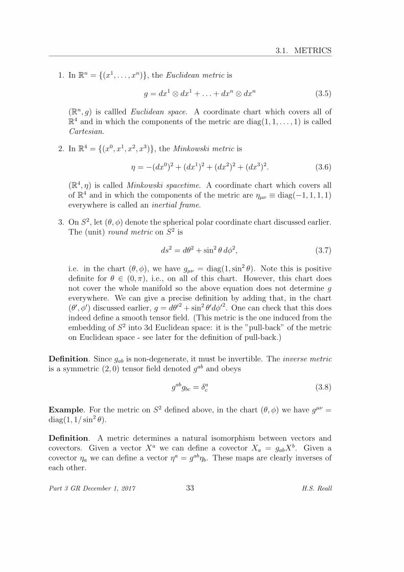
1. In Rn = (x1, . . . , xn), the Euclidean metric is
g = dx1 ⊗ dx1 + . . .+ dxn ⊗ dxn (3.5)
(Rn, g) is callled Euclidean space. A coordinate chart which covers all ofR4 and in which the components of the metric are diag(1, 1, . . . , 1) is calledCartesian.
2. In R4 = (x0, x1, x2, x3), the Minkowski metric is
η = −(dx0)2 + (dx1)2 + (dx2)2 + (dx3)2. (3.6)
(R4, η) is called Minkowski spacetime. A coordinate chart which covers allof R4 and in which the components of the metric are ηµν ≡ diag(−1, 1, 1, 1)everywhere is called an inertial frame.
3. On S2, let (θ, φ) denote the spherical polar coordinate chart discussed earlier.The (unit) round metric on S2 is
ds2 = dθ2 + sin2 θ dφ2, (3.7)
i.e. in the chart (θ, φ), we have gµν = diag(1, sin2 θ). Note this is positivedefinite for θ ∈ (0, π), i.e., on all of this chart. However, this chart doesnot cover the whole manifold so the above equation does not determine geverywhere. We can give a precise definition by adding that, in the chart(θ′, φ′) discussed earlier, g = dθ′2 + sin2 θ′dφ′2. One can check that this doesindeed define a smooth tensor field. (This metric is the one induced from theembedding of S2 into 3d Euclidean space: it is the ”pull-back” of the metricon Euclidean space - see later for the definition of pull-back.)
Definition. Since gab is non-degenerate, it must be invertible. The inverse metricis a symmetric (2, 0) tensor field denoted gab and obeys
gabgbc = δac (3.8)
Example. For the metric on S2 defined above, in the chart (θ, φ) we have gµν =diag(1, 1/ sin2 θ).
Definition. A metric determines a natural isomorphism between vectors andcovectors. Given a vector Xa we can define a covector Xa = gabX
b. Given acovector ηa we can define a vector ηa = gabηb. These maps are clearly inverses ofeach other.
Part 3 GR December 1, 2017 33 H.S. Reall
CHAPTER 3. THE METRIC TENSOR
Remark. This isomorphism is the reason why covectors are not more familiar:we are used to working in Euclidean space using Cartesian coordinates, for whichgµν and gµν are both the identity matrix, so the isomorphism appears trivial.
Definition. For a general tensor, abstract indices can be ”lowered” by contractingwith gab and ”raised” by contracting with gab. Raising and lowering preserve theordering of indices. The resulting tensor will be denoted by the same letter as theoriginal tensor.
Example. Let T be a (3, 2) tensor. Then T abcde = gbfg
dhgejT afchj.
3.2 Lorentzian signature
Remark. On a Lorentzian manifold, we take basis indices µ, ν, . . . to run from 0to n− 1.
At any point p of a Lorentzian manifold, we can choose an orthonormal basiseµ so that g(eµ, eν) = ηµν ≡ diag(−1, 1, . . . , 1). Such a basis is far from unique.If e′µ = (A−1)νµeν is any other such basis then we have
ηµν = g(e′µ, e′ν) = (A−1)ρµ(A−1)σνg(eρ, eσ) = (A−1)ρµ(A−1)σνηρσ. (3.9)
HenceηµνA
µρA
νσ = ηρσ. (3.10)
These are the defining equations of a Lorentz transformation in special relativity.Hence different orthonormal bases at p are related by Lorentz transformations. Wesaw earlier that the components of a vector at p transform as X ′µ = AµνX
ν . Weare starting to recover the structure of special relativity locally, as required by theEquivalence Principle.
Definition. On a Lorentzian manifold (M, g), a non-zero vector X ∈ Tp(M)is timelike if g(X,X) < 0, null (or lightlike) if g(X,X) = 0, and spacelike ifg(X,X) > 0.
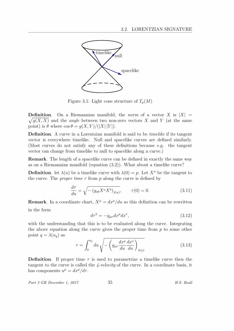
Remark. In an orthonormal basis at p, the metric has components ηµν so thetangent space at p has exactly the same structure as Minkowski spacetime, i.e.,null vectors at p define a light cone that separates timelike vectors at p fromspacelike vectors at p (see Fig. 3.1).
Exercise. Let Xa, Y b be non-zero vectors at p that are orthogonal, i.e., gabXaY b =
0. Show that (i) if Xa is timelike then Y a is spacelike; (ii) if Xa is null then Y a isspacelike or null; (iii) if Xa is spacelike then Y a can be spacelike, timelike, or null.(Hint. Choose an orthonormal basis to make the components of Xa as simple aspossible.)
Part 3 GR December 1, 2017 34 H.S. Reall
3.2. LORENTZIAN SIGNATURE
spacelike
nulltimelike
Figure 3.1: Light cone structure of Tp(M)
Definition. On a Riemannian manifold, the norm of a vector X is |X| =√g(X,X) and the angle between two non-zero vectors X and Y (at the same
point) is θ where cos θ = g(X, Y )/(|X| |Y |).Definition. A curve in a Lorentzian manifold is said to be timelike if its tangentvector is everywhere timelike. Null and spacelike curves are defined similarly.(Most curves do not satisfy any of these definitions because e.g. the tangentvector can change from timelike to null to spacelike along a curve.)
Remark. The length of a spacelike curve can be defined in exactly the same wayas on a Riemannian manifold (equation (3.2)). What about a timelike curve?
Definition. let λ(u) be a timelike curve with λ(0) = p. Let Xa be the tangent tothe curve. The proper time τ from p along the curve is defined by
dτ
du=√− (gabXaXb)λ(u), τ(0) = 0. (3.11)
Remark. In a coordinate chart, Xµ = dxµ/du so this definition can be rewritten
in the formdτ 2 = −gµνdxµdxν , (3.12)
with the understanding that this is to be evaluated along the curve. Integratingthe above equation along the curve gives the proper time from p to some otherpoint q = λ(uq) as
τ =
∫ uq
0
du
√−(gµν
dxµ
du
dxν
du
)λ(u)
(3.13)
Definition. If proper time τ is used to parametrize a timelike curve then thetangent to the curve is called the 4-velocity of the curve. In a coordinate basis, ithas components uµ = dxµ/dτ .
Part 3 GR December 1, 2017 35 H.S. Reall
CHAPTER 3. THE METRIC TENSOR
Remark. (3.12) implies that 4-velocity is a unit timelike vector:
gabuaub = −1. (3.14)
3.3 Curves of extremal proper time
Consider the following question. Let p and q be points connected by a timelikecurve. A small deformation of a timelike curve remains timelike hence there existinfinitely many timelike curves connecting p and q. The proper time between pand q will be different for different curves. Which curve extremizes the propertime between p and q?
This is a standard Euler-Lagrange problem. Consider timelike curves from pto q with parameter u such that λ(0) = p, λ(1) = q. Let’s use a dot to denote aderivative with respect to u. The proper time between p and q along such a curveis given by the functional
τ [λ] =
∫ 1
0
duG (x(u), x(u)) (3.15)
where
G (x(u), x(u)) ≡√−gµν(x(u))xµ(u)xν(u) (3.16)
and we are writing xµ(u) as a shorthand for xµ(λ(u)).The curve that extremizes the proper time, must satisfy the Euler-Lagrange
equationd
du
(∂G
∂xµ
)− ∂G
∂xµ= 0 (3.17)
Working out the various terms, we have (using the symmetry of the metric)
∂G
∂xµ= − 1
2G2gµν x
ν = − 1
Ggµν x
ν (3.18)
∂G
∂xµ= − 1
2Ggνρ,µ x
ν xρ (3.19)
where we have relabelled some dummy indices, and introduced the importantnotation of a comma to denote partial differentiation:
gνρ,µ ≡∂
∂xµgνρ (3.20)
We will be using this notation a lot henceforth.So far, our parameter u has been arbitrary subject to the conditions u(0) = p
and u(1) = q. At this stage, it is convenient to use a more physical parameter,
Part 3 GR December 1, 2017 36 H.S. Reall
3.3. CURVES OF EXTREMAL PROPER TIME
namely τ , the proper time along the curve. (Note that we could not have usedτ from the outset since the value of τ at q is different for different curves, whichwould make the range of integration different for different curves.) The paramersare related by (
dτ
du
)2
= −gµν xµxν = G2 (3.21)
and hence dτ/du = G. So in our equations above, we can replace d/du withGd/dτ , so the Euler-Lagrange equation becomes (after cancelling a factor of −G)
d
dτ
(gµν
dxν
dτ
)− 1
2gνρ,µ
dxν
dτ
dxρ
dτ= 0 (3.22)
Hence
gµνd2xν
dτ 2+ gµν,ρ
dxρ
dτ
dxν
dτ− 1
2gνρ,µ
dxν
dτ
dxρ
dτ= 0 (3.23)
In the second term, we can replace gµν,ρ with gµ(ν,ρ) because it is contracted withan object symmetrical on ν and ρ. Finally, contracting the whole expression withthe inverse metric and relabelling indices gives
d2xµ
dτ 2+ Γµνρ
dxν
dτ
dxρ
dτ= 0 (3.24)
where Γµνρ are known as the Christoffel symbols, and are defined by
Γµνρ =1
2gµσ (gσν,ρ + gσρ,ν − gνρ,σ) . (3.25)
Remarks. 1. Γµνρ = Γµρν . 2. The Christoffel symbols are not tensor components.
Neither the first term nor the second term in (3.24) are components of a vectorbut the sum of these two terms does give vector components. More about thissoon. 3. Equation 3.24 is called the geodesic equation. Geodesics will be definedbelow.
Example. In Minkowski spacetime, the components of the metric in an inertialframe are constant so Γµνρ = 0. Hence the above equation reduces to d2xµ/dτ 2 = 0.This is the equation of motion of a free particle! Hence, in Minkowski spacetime,the free particle trajectory between two (timelike separated) points p and q ex-tremizes the proper time between p and q.
This motivates the following postulate of General Relativity:
Postulate. Massive test bodies follow curves of extremal proper time, i.e., solu-tions of equation (3.24).
Part 3 GR December 1, 2017 37 H.S. Reall
CHAPTER 3. THE METRIC TENSOR
Remarks. 1. Massless particles obey a very similar equation which we shall dis-cuss shortly. 2. In Minkowski spacetime, curves of extremal proper time maximizethe proper time between two points. In a curved spacetime, this is true only locally,i.e., for any point p there exists a neighbourhood of p within which it is true.
Exercises
1. Show that (3.24) can be obtained more directly as the Euler-Lagrange equa-tion for the Lagrangian
L = −gµν(x(τ))dxµ
dτ
dxν
dτ(3.26)
This is usually the easiest way to derive (3.24) or to calculate the Christoffelsymbols.
2. Note that L has no explicit τ dependence, i.e., ∂L/∂τ = 0. Show that thisimplies that the following quantity is conserved along curves of extremalproper time (i.e. that is is annihilated by d/dτ):
L− ∂L
∂(dxµ/dτ)
dxµ
dτ= gµν
dxµ
dτ
dxν
dτ(3.27)
This is a check on the consistency of (3.24) because the definition of τ asproper time implies that the RHS must be −1.
Example. The Schwarzschild metric in Schwarzschild coordinates (t, r, θ, φ) is
ds2 = −fdt2 + f−1dr2 + r2dθ2 + r2 sin2 θ dφ2, f = 1− 2M
r(3.28)
where M is a constant. We have
L = f
(dt
dτ
)2
− f−1
(dr
dτ
)2
− r2
(dθ
dτ
)2
− r2 sin2 θ
(dφ
dτ
)2
(3.29)
so the EL equation for t(τ) is
d
dτ
(2fdt
dτ
)= 0 ⇒ d2t
dτ 2+ f−1f ′
dt
dτ
dr
dτ= 0 (3.30)
From this we can read off
Γ001 = Γ0
10 =f ′
2f, Γ0
µν = 0 otherwise (3.31)
The other Christoffel symbols are obtained in a similar way from the remainingEL equations (examples sheet 1).
Part 3 GR December 1, 2017 38 H.S. Reall
Chapter 4
Covariant derivative
4.1 Introduction
To formulate physical laws, we need to be able to differentiate tensor fields. Forscalar fields, partial differentiation is fine: f,µ ≡ ∂f/∂xµ are the components of thecovector field (df)a. However, for tensor fields, partial differentiation is no goodbecause the partial derivative of a tensor field does not give another tensor field:
Exercise. Let V a be a vector field. In any coordinate chart, let T µν = V µ,ν ≡
∂V µ/∂xν . Show that T µν do not transform as tensor components under a changeof chart.
The problem is that differentiation involves comparing a tensor at two infinites-imally nearby points of the manifold. But we have seen that this does not makesense: tensors at different points belong to different spaces. The mathematicalstructure that overcomes this difficulty is called a covariant derivative or connec-tion.
Definition. A covariant derivative ∇ on a manifold M is a map sending everypair of smooth vector fields X, Y to a smooth vector field ∇XY , with the followingproperties (where X, Y, Z are vector fields and f, g are functions)
∇fX+gYZ = f∇XZ + g∇YZ, (4.1)
∇X(Y + Z) = ∇XY +∇XZ, (4.2)
∇X(fY ) = f∇XY + (∇Xf)Y, (Leibniz rule), (4.3)
where the action of ∇ on functions is defined by
∇Xf = X(f). (4.4)
Remark. (4.1) implies that, at any point, the map ∇Y : X 7→ ∇XY is a linear
39
CHAPTER 4. COVARIANT DERIVATIVE
map from Tp(M) to itself. Hence it defines a (1, 1) tensor (see examples sheet1). More precisely, if η ∈ T ∗p (M) and X ∈ Tp(M) then we define (∇Y )(η,X) ≡η(∇XY ).
Definition. let Y be a vector field. The covariant derivative of Y is the (1, 1)tensor field ∇Y . In abstract index notation we usually write (∇Y )ab as ∇bY
a orY a
;b
Remarks.
1. Similarly we define ∇f : X 7→ ∇Xf = X(f). Hence ∇f = df . We can writethis as either ∇af or f;a or ∂af or f,a (i.e. the covariant derivative reducesto the partial derivative when acting on a function).
2. Does the map ∇ : X, Y 7→ ∇XY define a (1, 2) tensor field? No - equation(4.3) shows that this map is not linear in Y .
Example. Pick a coordinate chart on M . Let ∇ be the partial derivative in thischart. This satisfies all of the above conditions. This is not a very interestingexample of a covariant derivative because it depends on choosing a particularchart: if we use a different chart then this covariant derivative will not be thepartial derivative in the new chart.
Definition. In a basis eµ the connection components Γµνρ are defined by
∇ρeν ≡ ∇eρeν = Γµνρeµ (4.5)
Example. The Christoffel symbols are the coordinate basis components of acertain connection, the Levi-Civita connection, which is defined on any manifoldwith a metric. More about this soon.
Write X = Xµeµ and Y = Y µeµ. Now
∇XY = ∇X(Y µeµ) = X(Y µ)eµ + Y µ∇Xeµ (Leibniz)
= Xνeν(Yµ)eµ + Y µ∇Xνeνeµ
= Xνeν(Yµ)eµ + Y µXν∇νeµ by (4.1)
= Xνeν(Yµ)eµ + Y µXνΓρµνeρ
= Xν(eν(Y
µ) + ΓµρνYρ)eµ (4.6)
and hence(∇XY )µ = Xνeν(Y
µ) + ΓµρνYρXν (4.7)
soY µ
;ν = eν(Yµ) + ΓµρνY
ρ (4.8)
Part 3 GR December 1, 2017 40 H.S. Reall
4.1. INTRODUCTION
In a coordinate basis, this reduces to
Y µ;ν = Y µ
,ν + ΓµρνYρ (4.9)
The connection components Γµνρ are not tensor components:
Exercise (examples sheet 2). Consider a change of basis e′µ = (A−1)νµeν . Showthat
Γ′µνρ = Aµτ (A
−1)λν(A−1)σρΓ
τλσ + Aµτ (A
−1)σρeσ((A−1)τ ν) (4.10)
The presence of the second term demonstrates that Γµνρ are not tensor components.Hence neither term in the RHS of equation (4.9) transforms as a tensor. However,the sum of these two terms does transform as a tensor.
Exercise. Let ∇ and ∇ be two different connections on M . Show that ∇− ∇ isa (1, 2) tensor field. You can do this either from the definition of a connection, orfrom the transformation law for the connection components.
The action of ∇ is extended to general tensor fields by the Leibniz property.If T is a tensor field of type (r, s) then ∇T is a tensor field of type (r, s+ 1). Forexample, if η is a covector field then, for any vector fields X and Y , we define
(∇Xη)(Y ) ≡ ∇X(η(Y ))− η(∇XY ). (4.11)
It is not obvious that this defines a (0, 2) tensor but we can see this as follows:
(∇Xη)(Y ) = ∇X(ηµYµ)− ηµ(∇XY )µ
= X(ηµ)Y µ + ηµX(Y µ)− ηµ(Xνeν(Y
µ) + ΓµρνYρXν
), (4.12)
where we used (4.7). Now, the second and third terms cancel (X = Xνeν) andhence (renaming dummy indices in the final term)
(∇Xη)(Y ) =(X(ηµ)− ΓρµνηρX
ν)Y µ, (4.13)
which is linear in Y µ so ∇Xη is a covector field with components
(∇Xη)µ = X(ηµ)− ΓρµνηρXν
= Xν(eν(ηµ)− Γρµνηρ
)(4.14)
This is linear in Xν and hence ∇η is a (0, 2) tensor field with components
ηµ;ν = eν(ηµ)− Γρµνηρ (4.15)
In a coordinate basis, this is
ηµ;ν = ηµ,ν − Γρµνηρ (4.16)
Part 3 GR December 1, 2017 41 H.S. Reall
CHAPTER 4. COVARIANT DERIVATIVE
Now the Leibniz rule can be used to obtain the formula for the coordinate basiscomponents of ∇T where T is a (r, s) tensor:
T µ1...µrν1...νs;ρ = T µ1...µrν1...νs,ρ + Γµ1σρTσµ2...µr
ν1...νs + . . .+ ΓµrσρTµ1...µr−1σ
ν1...νs
− Γσν1ρTµ1...µr
σν2...νs − . . .− ΓσνsρTµ1...µr
ν1...νs−1σ (4.17)
Exercise. Prove this result for a (1, 1) tensor.
Remark. We are using a comma and semi-colon to denote partial, and covariant,derivatives respectively. If more than one index appears after a comma or semi-colon then the derivative is to be taken with respect to all indices. The indexnearest to comma/semi-colon is the first derivative to be taken. For example,f,µν = f,µ,ν ≡ ∂ν∂µf , and Xa
;bc = ∇c∇bXa (we cannot use abstract indices for the
first example since it is not a tensor). The second partial derivatives of a functioncommute: f,µν = f,νµ but for a covariant derivative this is not true in general. Setη = df in (4.16) to get, in a coordinate basis,
f;µν = f,µν − Γρµνf,ρ (4.18)
Antisymmetrizing gives
f;[µν] = −Γρ[µν]f,ρ (coordinate basis) (4.19)
Definition. A connection ∇ is torsion-free if ∇a∇bf = ∇b∇af for any function
f . From (4.19), this is equivalent to
Γρ[µν] = 0 (coordinate basis) (4.20)
Lemma. For a torsion-free connection, if X and Y are vector fields then
∇XY −∇YX = [X, Y ] (4.21)
Proof. Use a coordinate basis:
XνY µ;ν − Y νXµ
;ν = XνY µ,ν + ΓµρνX
νY ρ − Y νXµ,ν − ΓµρνY
νXρ
= [X, Y ]µ + 2Γµ[ρν]XνY ρ
= [X, Y ]µ (4.22)
Hence the equation is true in a coordinate basis and therefore (as it is a tensorequation) it is true in any basis.
Remark. Even with zero torsion, the second covariant derivatives of a tensor fielddo not commute. More soon.
Part 3 GR December 1, 2017 42 H.S. Reall
4.2. THE LEVI-CIVITA CONNECTION
4.2 The Levi-Civita connection
On a manifold with a metric, the metric singles out a preferred connection:
Theorem. Let M be a manifold with a metric g. There exists a unique torsion-freeconnection ∇ such that the metric is covariantly constant: ∇g = 0 (i.e. gab;c = 0).This is called the Levi-Civita (or metric) connection.
Proof. Let X, Y, Z be vector fields then
X(g(Y, Z)) = ∇X(g(Y, Z)) = g(∇XY, Z) + g(Y,∇XZ), (4.23)
where we used the Leibniz rule and ∇Xg = 0 in the second equality. PermutingX, Y, Z leads to two similar identities:
Y (g(Z,X)) = g(∇YZ,X) + g(Z,∇YX), (4.24)
Z(g(X, Y )) = g(∇ZX, Y ) + g(X,∇ZY ), (4.25)
Add the first two of these equations and subtract the third to get (using thesymmetry of the metric)
X(g(Y, Z)) + Y (g(Z,X))− Z(g(X, Y )) = g(∇XY +∇YX,Z)
− g(∇ZX −∇XZ, Y )
+ g(∇YZ −∇ZY,X) (4.26)
The torsion-free condition implies
∇XY −∇YX = [X, Y ] (4.27)
Using this and the same identity with X, Y, Z permuted gives
X(g(Y, Z)) + Y (g(Z,X))− Z(g(X, Y )) = 2g(∇XY, Z)− g([X, Y ], Z)
− g([Z,X], Y ) + g([Y, Z], X)
(4.28)
Hence
g(∇XY, Z) =1
2[X(g(Y, Z)) + Y (g(Z,X))− Z(g(X, Y ))
+ g([X, Y ], Z) + g([Z,X], Y )− g([Y, Z], X)] (4.29)
This determines ∇XY uniquely because the metric is non-degenerate. It remainsto check that it satisfies the properties of a connection. For example:
g(∇fXY, Z) =1
2[fX(g(Y, Z)) + Y (fg(Z,X))− Z(fg(X, Y ))
Part 3 GR December 1, 2017 43 H.S. Reall
CHAPTER 4. COVARIANT DERIVATIVE
+ g([fX, Y ], Z) + g([Z, fX], Y )− fg([Y, Z], X)]
=1
2[fX(g(Y, Z)) + fY (g(Z,X)) + Y (f)g(Z,X)
− fZ(g(X, Y ))− Z(f)g(X, Y ) + fg([X, Y ], Z)− Y (f)g(X,Z)
+ fg([Z,X], Y ) + Z(f)g(X, Y )− fg([Y, Z], X)]
=f
2[X(g(Y, Z)) + Y (g(Z,X))− Z(g(X, Y ))
+ g([X, Y ], Z) + g([Z,X], Y )− g([Y, Z], X)]
= fg(∇XY, Z) = g(f∇XY, Z) (4.30)
and hence g(∇fXY−f∇XY, Z) = 0 for any vector field Z so, by the non-degeneracyof the metric, ∇fXY = f∇XY .
Exercise. Show that ∇XY as defined by (4.29) satisfies the other propertiesrequired of a connection.
Remark. In differential geometry, this theorem is called the fundamental theoremof Riemannian geometry (although it applies for a metric of any signature).
Let’s determine the components of the Levi-Civita connection in a coordinatebasis (for which [eµ, eν ] = 0):
g(∇ρeν , eσ) =1
2[eρ(gνσ) + eν(gσρ)− eσ(gρν)] , (4.31)
that is
g(Γτνρeτ , eσ) =1
2(gσν,ρ + gσρ,ν − gνρ,σ) (4.32)
The LHS is just Γτνρgτσ. Hence if we multiply the whole equation by the inversemetric gµσ we obtain
Γµνρ =1
2gµσ (gσν,ρ + gσρ,ν − gνρ,σ) (4.33)
This is the same equation as we obtained earlier; we have now shown that theChristoffel symbols are the components of the Levi-Civita connection.
Remark. In GR, we take the connection to be the Levi-Civita connection. Thisis not as restrictive as it sounds: we saw above that the difference between twoconnections is a tensor field. Hence we can write any connection (even one withtorsion) in terms of the Levi-Civita connection and a (1, 2) tensor field. In GR wecould regard the latter as a particular kind of ”matter” field, rather than as partof the geometry of spacetime.
Part 3 GR December 1, 2017 44 H.S. Reall
4.3. GEODESICS
4.3 Geodesics
Previously we considered curves that extremize the proper time between two pointsof a spacetime, and showed that this gives the equation
d2xµ
dτ 2+ Γµνρ(x(τ))
dxν
dτ
dxρ
dτ= 0, (4.34)
where τ is the proper time along the curve. The tangent vector to the curve hascomponents Xµ = dxµ/dτ . This is defined only along the curve. However, wecan extend Xµ (in an arbitrary way) to a neighbourhood of the curve, so that Xµ
becomes a vector field, and the curve is an integral curve of this vector field. Thechain rule gives
d2xµ
dτ 2=dXµ(x(τ))
dτ=dxν
dτ
∂Xµ
∂xν= XνXµ
,ν . (4.35)
Note that the LHS is independent of how we extend Xµ hence so must be theRHS. We can now write (4.34) as
Xν(Xµ
,ν + ΓµνρXρ)
= 0 (4.36)
which is the same as
XνXµ;ν = 0, or ∇XX = 0. (4.37)
where we are using the Levi-Civita connection. We now extend this to an arbitraryconnection:
Definition. Let M be a manifold with a connection ∇. An affinely parameterizedgeodesic is an integral curve of a vector field X satisfying ∇XX = 0.
Remarks.
1. What do we mean by ”affinely parameterized”? Consider a curve with pa-rameter t whose tangent X satisfies the above definition. Let u be someother parameter for the curve, so t = t(u) and dt/du > 0. Then the tangentvector becomes Y = hX where h = dt/du. Hence
∇Y Y = ∇hX(hX) = h∇X(hX) = h2∇XX +X(h)hX = fY, (4.38)
where f = X(h) = dh/dt. Hence ∇Y Y = fY describes the same geodesic.In this case, the geodesic is not affinely parameterized.
It always is possible to find an affine parameter so there is no loss of gen-erality in restricting to affinely parameterized geodesics. Note that the newparameter also is affine iff X(h) = 0, i.e., h is constant. Then u = at+b wherea and b are constants with a > 0 (a = h−1). Hence there is a 2-parameterfamily of affine parameters for any geodesic.
Part 3 GR December 1, 2017 45 H.S. Reall
CHAPTER 4. COVARIANT DERIVATIVE
2. Reversing the above steps shows that, in a coordinate chart, for any con-nection, the geodesic equation can be written as (4.34) with τ an arbitraryaffine parameter.
3. In GR, curves of extremal proper time are timelike geodesics (with ∇ theLevi-Civita connection). But one can also consider geodesics which are nottimelike. These satisfy (4.34) with τ an affine parameter. The easiest wayto obtain this equation is to use the Lagrangian (3.26).
Theorem. Let M be a manifold with a connection ∇. Let p ∈ M and Xp ∈Tp(M). Then there exists a unique affinely parameterized geodesic through p withtangent vector Xp at p.
Proof. Choose a coordinate chart xµ in a neighbourhood of p. Consider a curveparameterized by τ . It has tangent vector with components Xµ = dxµ/dτ . Thegeodesic equation is (4.34). We want the curve to satisfy the initial conditions
xµ(0) = xµp ,
(dxµ
dτ
)τ=0
= Xµp . (4.39)
This is a coupled system of n ordinary differential equations for the n functionsxµ(t). Existence and uniqueness is guaranteed by the standard theory of ordinarydifferential equations.
Exercise. Let X be tangent to an affinely parameterized geodesic of the Levi-Civita connection. Show that ∇X(g(X,X)) = 0 and hence g(X,X) is constantalong the geodesic. Therefore the tangent vector cannot change e.g. from timeliketo null along the geodesic: a geodesic is either timelike, spacelike or null.
Postulate. In GR, free particles move on geodesics (of the Levi-Civita connec-tion). These are timelike for massive particles, and null for massless particles (e.g.photons).
Remark. In the timelike case we can use proper time as an affine parameter.This imposes the additional restriction g(X,X) = −1. If τ and τ ′ both are propertimes along a geodesic then τ ′ = τ + b (i.e. a = 1 above). In other words, clocksmeasuring proper time differ only by their choice of zero. In particular, theymeasure equal time intervals. Similarly in the spacelike case (or on a Riemannianmanifold), we use arc length s as affine parameter, which gives g(X,X) = 1 ands′ = s+ b. In the null case, there is no analogue of proper time or arc length andso there is a 2-parameter ambiguity in affine parameterization.
Part 3 GR December 1, 2017 46 H.S. Reall
4.4. NORMAL COORDINATES
4.4 Normal coordinates
Definition. Let M be a manifold with a connection ∇. Let p ∈ M . The expo-nential map from Tp(M) to M is defined as the map which sends Xp to the pointunit affine parameter distance along the geodesic through p with tangent Xp at p.
Remark. It can be shown that this map is one-to-one and onto locally, i.e., forXp in a neighbourhood of the origin in Tp(M).
Exercise. Let 0 ≤ t ≤ 1. Show that the exponential map sends tXp to the pointaffine parameter distance t along the geodesic through p with tangent Xp at p.
Definition. Let eµ be a basis for Tp(M). Normal coordinates at p are definedin a neighbourhood of p as follows. Pick q near p. Then the coordinates of q areXµ where Xa is the element of Tp(M) that maps to q under the exponential map.
Lemma. Γµ(νρ)(p) = 0 in normal coordinates at p. For a torsion-free connection,
Γµνρ(p) = 0 in normal coordinates at p.Proof. From the above exercise, it follows that affinely parameterized geodesics
through p are given in normal coordinates by Xµ(t) = tXµp . Hence the geodesic
equation reduces toΓµνρ(X(t))Xν
pXρp = 0. (4.40)
Evaluating at t = 0 gives that Γµνρ(p)XνpX
ρp = 0. But Xp is arbitrary, so the first
result follows. The second result follows using the fact that torsion-free impliesΓµ[νρ] = 0 in a coordinate chart.
Remark. The connection components away from p will not vanish in general.
Lemma. On a manifold with a metric, if the Levi-Civita connection is used todefine normal coordinates at p then gµν,ρ = 0 at p.
Proof. Apply the previous lemma. We then have, at p,
0 = 2gµσΓσνρ = gµν,ρ + gµρ,ν − gνρ,µ (4.41)
Now symmetrize on µν: the final two terms cancel and the result follows.
Remark. Again, we emphasize, this is valid only at the point p. At any point,we can introduce normal coordinates to make the first partial derivatives of themetric vanish at that point. They will not vanish away for that point.
Lemma. On a manifold with metric one can choose normal coordinates at pso that gµν,ρ(p) = 0 and also gµν(p) = ηµν (Lorentzian case) or gµν(p) = δµν(Riemannian case).
Proof. We’ve already shown gµν,ρ(p) = 0. Consider ∂/∂X1. The integral curvethrough p of this vector field is Xµ(t) = (t, 0, 0, . . . , 0) (since Xµ = 0 at p). But,
Part 3 GR December 1, 2017 47 H.S. Reall
CHAPTER 4. COVARIANT DERIVATIVE
from the above, this is the same as the geodesic through p with tangent vector e1
at p. It follows that ∂/∂X1 = e1 at p (since both vectors are tangent to the curveat p). Similarly ∂/∂Xµ = eµ at p. But the choice of basis eµ was arbitrary. Sowe are free to choose eµ to be an orthonormal basis. ∂/∂Xµ then defines anorthonormal basis at p too.
In summary, on a Lorentzian (Riemannian) manifold, we can choose coordi-nates in the neighbourhood of any point p so that the components of the metric atp are the same as those of the Minkowski metric in inertial coordinates (Euclideanmetric in Cartesian coordinates), and the first partial derivatives of the metricvanish at p.
Definition. In a Lorentzian manifold a local inertial frame at p is a set of normalcoordinates at p with the above properties.
Thus the assumption that spacetime is a Lorentzian manifold leads to a precisemathematical definition of a local inertial frame.
Part 3 GR December 1, 2017 48 H.S. Reall
Chapter 5
Physical laws in curved spacetime
5.1 Minimal coupling, equivalence principle
Physical laws in curved spacetime should exhibit general covariance: they shouldbe independent of any choice of basis or coordinate chart. In special relativity,we restrict attention to coordinate systems corresponding to inertial frames. Thelaws of physics should exhibit special covariance, i.e, take the same form in anyinertial frame (this is the principle of relativity). The following procedure can beused to convert such laws of physics into generally covariant laws:
1. Replace the Minkowski metric by a curved spacetime metric.
2. Replace partial derivatives with covariant derivatives (associated to the Levi-Civita connection). This rule is called minimal coupling in analogy with asimilar rule for charged fields in electrodynamics.
3. Replace coordinate basis indices µ, ν etc (referring to an inertial frame) withabstract indices a, b etc.
Examples. Let xµ denote the coordinates of an inertial frame, and ηµν the inverseMinkowski metric (which has the same components as ηµν).
1. The simplest Lorentz invariant field equation is the wave equation for a scalarfield Φ
ηµν∂µ∂νΦ = 0. (5.1)
Follow the rules above to obtain the wave equation in a general spacetime:
gab∇a∇bΦ = 0, or ∇a∇aΦ = 0 or Φ;aa = 0. (5.2)
A simple generalization of this equation is the Klein-Gordon equation de-scribing a scalar field of mass m:
∇a∇aΦ−m2Φ = 0. (5.3)
49
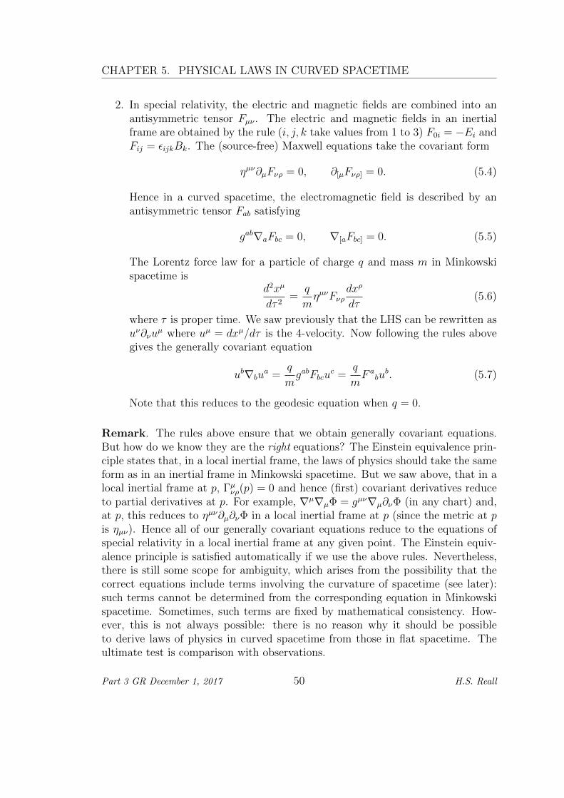
CHAPTER 5. PHYSICAL LAWS IN CURVED SPACETIME
2. In special relativity, the electric and magnetic fields are combined into anantisymmetric tensor Fµν . The electric and magnetic fields in an inertialframe are obtained by the rule (i, j, k take values from 1 to 3) F0i = −Ei andFij = εijkBk. The (source-free) Maxwell equations take the covariant form
ηµν∂µFνρ = 0, ∂[µFνρ] = 0. (5.4)
Hence in a curved spacetime, the electromagnetic field is described by anantisymmetric tensor Fab satisfying
gab∇aFbc = 0, ∇[aFbc] = 0. (5.5)
The Lorentz force law for a particle of charge q and mass m in Minkowskispacetime is
d2xµ
dτ 2=
q
mηµνFνρ
dxρ
dτ(5.6)
where τ is proper time. We saw previously that the LHS can be rewritten asuν∂νu
µ where uµ = dxµ/dτ is the 4-velocity. Now following the rules abovegives the generally covariant equation
ub∇bua =
q
mgabFbcu
c =q
mF a
bub. (5.7)
Note that this reduces to the geodesic equation when q = 0.
Remark. The rules above ensure that we obtain generally covariant equations.But how do we know they are the right equations? The Einstein equivalence prin-ciple states that, in a local inertial frame, the laws of physics should take the sameform as in an inertial frame in Minkowski spacetime. But we saw above, that in alocal inertial frame at p, Γµνρ(p) = 0 and hence (first) covariant derivatives reduceto partial derivatives at p. For example, ∇µ∇µΦ = gµν∇µ∂νΦ (in any chart) and,at p, this reduces to ηµν∂µ∂νΦ in a local inertial frame at p (since the metric at pis ηµν). Hence all of our generally covariant equations reduce to the equations ofspecial relativity in a local inertial frame at any given point. The Einstein equiv-alence principle is satisfied automatically if we use the above rules. Nevertheless,there is still some scope for ambiguity, which arises from the possibility that thecorrect equations include terms involving the curvature of spacetime (see later):such terms cannot be determined from the corresponding equation in Minkowskispacetime. Sometimes, such terms are fixed by mathematical consistency. How-ever, this is not always possible: there is no reason why it should be possibleto derive laws of physics in curved spacetime from those in flat spacetime. Theultimate test is comparison with observations.
Part 3 GR December 1, 2017 50 H.S. Reall
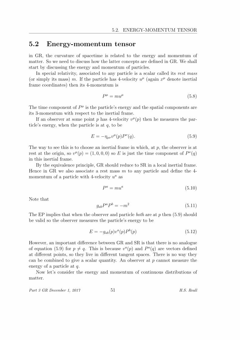
5.2. ENERGY-MOMENTUM TENSOR
5.2 Energy-momentum tensor
in GR, the curvature of spacetime is related to the energy and momentum ofmatter. So we need to discuss how the latter concepts are defined in GR. We shallstart by discussing the energy and momentum of particles.
In special relativity, associated to any particle is a scalar called its rest mass(or simply its mass) m. If the particle has 4-velocity uµ (again xµ denote inertialframe coordinates) then its 4-momentum is
P µ = muµ (5.8)
The time component of P µ is the particle’s energy and the spatial components areits 3-momentum with respect to the inertial frame.
If an observer at some point p has 4-velocity vµ(p) then he measures the par-ticle’s energy, when the particle is at q, to be
E = −ηµνvµ(p)P ν(q). (5.9)
The way to see this is to choose an inertial frame in which, at p, the observer is atrest at the origin, so vµ(p) = (1, 0, 0, 0) so E is just the time component of P ν(q)in this inertial frame.
By the equivalence principle, GR should reduce to SR in a local inertial frame.Hence in GR we also associate a rest mass m to any particle and define the 4-momentum of a particle with 4-velocity ua as
P a = mua (5.10)
Note that
gabPaP b = −m2 (5.11)
The EP implies that when the observer and particle both are at p then (5.9) shouldbe valid so the observer measures the particle’s energy to be
E = −gab(p)va(p)P b(p) (5.12)
However, an important difference between GR and SR is that there is no analogueof equation (5.9) for p 6= q. This is because va(p) and P a(q) are vectors definedat different points, so they live in different tangent spaces. There is no way theycan be combined to give a scalar quantity. An observer at p cannot measure theenergy of a particle at q.
Now let’s consider the energy and momentum of continuous distributions ofmatter.
Part 3 GR December 1, 2017 51 H.S. Reall
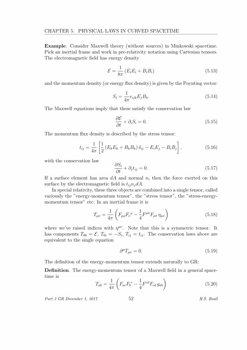
CHAPTER 5. PHYSICAL LAWS IN CURVED SPACETIME
Example. Consider Maxwell theory (without sources) in Minkowski spacetime.Pick an inertial frame and work in pre-relativity notation using Cartesian tensors.The electromagnetic field has energy density
E =1
8π(EiEi +BiBi) (5.13)
and the momentum density (or energy flux density) is given by the Poynting vector:
Si =1
4πεijkEjBk. (5.14)
The Maxwell equations imply that these satisfy the conservation law
∂E∂t
+ ∂iSi = 0. (5.15)
The momentum flux density is described by the stress tensor:
tij =1
4π
[1
2(EkEk +BkBk) δij − EiEj −BiBj
], (5.16)
with the conservation law∂Si∂t
+ ∂jtij = 0. (5.17)
If a surface element has area dA and normal ni then the force exerted on thissurface by the electromagnetic field is tijnjdA.
In special relativity, these three objects are combined into a single tensor, calledvariously the ”energy-momentum tensor”, the ”stress tensor”, the ”stress-energy-momentum tensor” etc. In an inertial frame it is
Tµν =1
4π
(FµρFν
ρ − 1
4F ρσFρσ ηµν
)(5.18)
where we’ve raised indices with ηµν . Note that this is a symmetric tensor. Ithas components T00 = E , T0i = −Si, Tij = tij. The conservation laws above areequivalent to the single equation
∂µTµν = 0. (5.19)
The definition of the energy-momentum tensor extends naturally to GR:
Definition. The energy-momentum tensor of a Maxwell field in a general space-time is
Tab =1
4π
(FacFb
c − 1
4F cdFcd gab
)(5.20)
Part 3 GR December 1, 2017 52 H.S. Reall
5.2. ENERGY-MOMENTUM TENSOR
Exercise (examples sheet 2). Show that Maxwell’s equations imply that
∇aTab = 0. (5.21)
In GR (and SR) we assume that continuous matter always is described by a con-served energy-momentum tensor:
Postulate. The energy, momentum, and stresses, of matter are described by anenergy-momentum tensor, a (0, 2) symmetric tensor Tab that is conserved: ∇aTab =0.
Remark. Let ua be the 4-velocity of an observer O at p. Consider a local inertialframe (LIF) at p in which O is at rest. Choose an orthonormal basis at p eµaligned with the coordinate axes of this LIF. In such a basis, ea0 = ua. Denotethe spatial basis vectors as eai , i = 1, 2, 3. From the Einstein equivalence principle,E ≡ T00 = Tabe
a0eb0 = Tabu
aub is the energy density of matter at p measured byO. Similarly, Si ≡ −T0i is the momentum density and tij ≡ Tij the stress tensormeasured by O. The energy-momentum current measured by O is the 4-vectorja = −T abub, which has components (E , Si) in this basis.
Remark. In an inertial frame xµ in Minkowski spacetime, local conservation ofTab is equivalent to equations of the form (5.15) and (5.17). If one integratesthese over a fixed volume V in surfaces of constant t = x0 then one obtains globalconservation equations. For example, integrating (5.15) over V gives
d
dt
∫V
E = −∫S
S · ndA (5.22)
where the surface S (with outward unit normal n) bounds V . In words: the rateof increase of the energy of matter in V is equal to minus the energy flux acrossS. In a general curved spacetime, such an interpretation is not possible. This isbecause the gravitational field can do work on the matter in the spacetime. Onemight think that one could obtain global conservation laws in curved spacetime byintroducing a definition of energy density etc for the gravitational field. This is asubtle issue. The gravitational field is described by the metric gab. In Newtoniantheory, the energy density of the gravitational field is −(1/8π)(∇Φ)2 so one mightexpect that in GR the energy density of the gravitational field should be someexpression quadratic in first derivatives of gab. But we have seen that we canchoose normal coordinates to make the first partial derivatives of gab vanish atany given point. Gravitational energy certainly exists but not in a local sense.For example one can define the total energy (i.e. the energy of matter and thegravitational field) for certain spacetimes (this will be discussed in the black holescourse).
Part 3 GR December 1, 2017 53 H.S. Reall
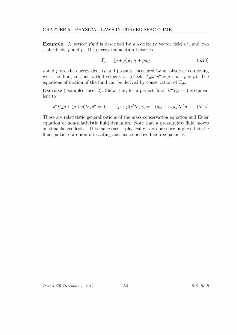
CHAPTER 5. PHYSICAL LAWS IN CURVED SPACETIME
Example. A perfect fluid is described by a 4-velocity vector field ua, and twoscalar fields ρ and p. The energy-momentum tensor is
Tab = (ρ+ p)uaub + pgab (5.23)
ρ and p are the energy density and pressure measured by an observer co-movingwith the fluid, i.e., one with 4-velocity ua (check: Tabu
aub = ρ + p − p = ρ). Theequations of motion of the fluid can be derived by conservation of Tab:
Exercise (examples sheet 2). Show that, for a perfect fluid, ∇aTab = 0 is equiva-lent to
ua∇aρ+ (ρ+ p)∇aua = 0, (ρ+ p)ub∇bua = −(gab + uaub)∇bp (5.24)
These are relativistic generalizations of the mass conservation equation and Eulerequation of non-relativistic fluid dynamics. Note that a pressureless fluid moveson timelike geodesics. This makes sense physically: zero pressure implies that thefluid particles are non-interacting and hence behave like free particles.
Part 3 GR December 1, 2017 54 H.S. Reall
Chapter 6
Curvature
6.1 Parallel transport
On a general manifold there is no way of comparing tensors at different points. Forexample, we can’t say whether a vector at p is the same as a vector at q. However,with a connection we can define a notion of ”a tensor that doesn’t change along acurve”:
Definition. Let Xa be the tangent to a curve. A tensor field T is parallellytransported along the curve if ∇XT = 0.
Remarks.
1. Sometimes we say ”parallelly propagated” instead of ”parallelly transported”.
2. A geodesic is a curve whose tangent vector is parallelly transported alongthe curve.
3. Let p be a point on a curve. If we specify T at p then the above equationdetermines T uniquely everywhere along the curve. For example, considera (1, 1) tensor. Introduce a chart in a neighbourhood of p. Let t be theparameter along the curve. In a coordinate chart, Xµ = dxµ/dt so ∇XT = 0gives
0 = XσT µν;σ = XσT µν,σ + ΓµρσTρνX
σ − ΓρνσTµρX
σ
=dT µνdt
+ ΓµρσTρνX
σ − ΓρνσTµρX
σ (6.1)
Standard ODE theory guarantees a unique solution given initial values forthe components T µν .
55
CHAPTER 6. CURVATURE
4. If q is some other point on the curve then parallel transport along a curvefrom p to q determines an isomorphism between tensors at p and tensors atq.
Consider Euclidean space or Minkowski spacetime with the Levi-Civita connection,and use Cartesian/inertial frame coordinates so the Christoffel symbols vanish ev-erywhere. Then a tensor is parallelly transported along a curve iff its componentsare constant along the curve. Hence if we have two different curves from p to q thenthe result of parallelly transporting T from p to q is independent of which curvewe choose. However, in a general spacetime this is no longer true: parallel trans-port is path-dependent. The path-dependence of parallel transport is measuredby the Riemann curvature tensor. For Euclidean space or Minkowski spacetime,the Riemann tensor (of the Levi-Civita connection) vanishes and we say that thespacetime is flat.
6.2 The Riemann tensor
We shall return to the path-dependence of parallel transport below. First we definethe Riemann tensor is as follows:
Definition. The Riemann curvature tensor Rabcd of a connection ∇ is defined by
RabcdZ
bXcY d = (R(X, Y )Z)a, where X, Y, Z are vector fields and R(X, Y )Z is thevector field
R(X, Y )Z = ∇X∇YZ −∇Y∇XZ −∇[X,Y ]Z (6.2)
To demonstrate that this defines a tensor, we need to show that it is linear inX, Y, Z. The symmetry R(X, Y )Z = −R(Y,X)Z implies that we need only checklinearity in X and Z. The non-trivial part is to check what happens if we multiplyX or Z by a function f :
R(fX, Y )Z = ∇fX∇YZ −∇Y∇fXZ −∇[fX,Y ]Z
= f∇X∇YZ −∇Y (f∇XZ)−∇f [X,Y ]−Y (f)XZ
= f∇X∇YZ − f∇Y∇XZ − Y (f)∇XZ −∇f [X,Y ]Z +∇Y (f)XZ
= f∇X∇YZ − f∇Y∇XZ − Y (f)∇XZ − f∇[X,Y ]Z + Y (f)∇XZ
= fR(X, Y )Z (6.3)
R(X, Y )(fZ) = ∇X∇Y (fZ)−∇Y∇X(fZ)−∇[X,Y ](fZ)
= ∇X(f∇YZ + Y (f)Z)−∇Y (f∇XZ +X(f)Z)
−f∇[X,Y ]Z − [X, Y ](f)Z
= f∇X∇YZ +X(f)∇YZ + Y (f)∇XZ +X(Y (f))Z
Part 3 GR December 1, 2017 56 H.S. Reall
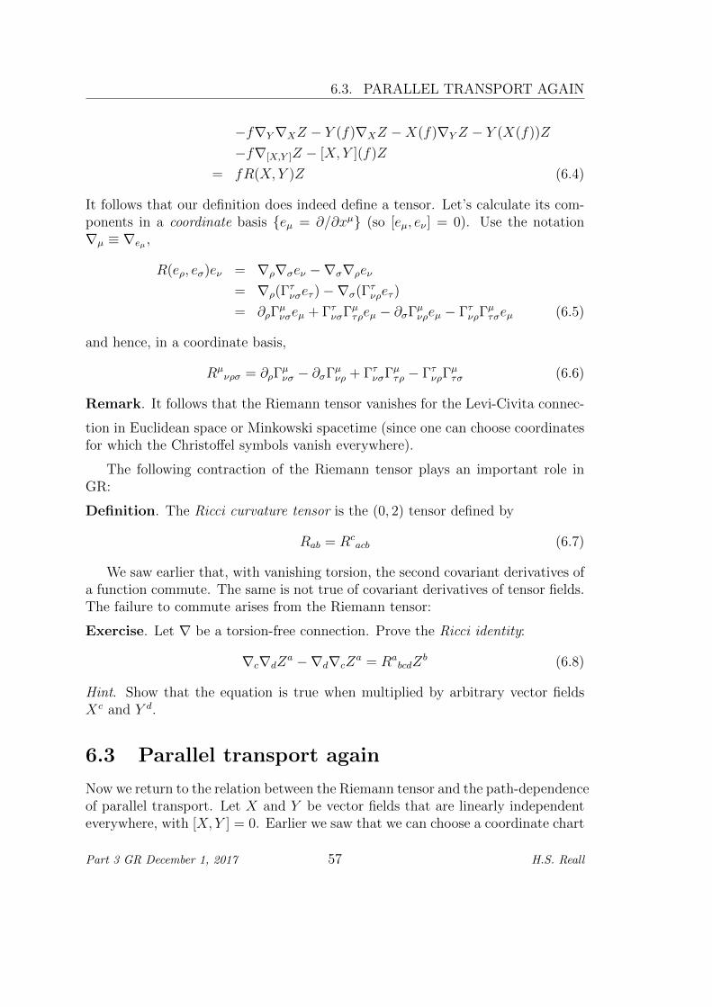
6.3. PARALLEL TRANSPORT AGAIN
−f∇Y∇XZ − Y (f)∇XZ −X(f)∇YZ − Y (X(f))Z
−f∇[X,Y ]Z − [X, Y ](f)Z
= fR(X, Y )Z (6.4)
It follows that our definition does indeed define a tensor. Let’s calculate its com-ponents in a coordinate basis eµ = ∂/∂xµ (so [eµ, eν ] = 0). Use the notation∇µ ≡ ∇eµ ,
R(eρ, eσ)eν = ∇ρ∇σeν −∇σ∇ρeν
= ∇ρ(Γτνσeτ )−∇σ(Γτνρeτ )
= ∂ρΓµνσeµ + ΓτνσΓµτρeµ − ∂σΓµνρeµ − ΓτνρΓ
µτσeµ (6.5)
and hence, in a coordinate basis,
Rµνρσ = ∂ρΓ
µνσ − ∂σΓµνρ + ΓτνσΓµτρ − ΓτνρΓ
µτσ (6.6)
Remark. It follows that the Riemann tensor vanishes for the Levi-Civita connec-
tion in Euclidean space or Minkowski spacetime (since one can choose coordinatesfor which the Christoffel symbols vanish everywhere).
The following contraction of the Riemann tensor plays an important role inGR:
Definition. The Ricci curvature tensor is the (0, 2) tensor defined by
Rab = Rcacb (6.7)
We saw earlier that, with vanishing torsion, the second covariant derivatives ofa function commute. The same is not true of covariant derivatives of tensor fields.The failure to commute arises from the Riemann tensor:
Exercise. Let ∇ be a torsion-free connection. Prove the Ricci identity:
∇c∇dZa −∇d∇cZ
a = RabcdZ
b (6.8)
Hint. Show that the equation is true when multiplied by arbitrary vector fieldsXc and Y d.
6.3 Parallel transport again
Now we return to the relation between the Riemann tensor and the path-dependenceof parallel transport. Let X and Y be vector fields that are linearly independenteverywhere, with [X, Y ] = 0. Earlier we saw that we can choose a coordinate chart
Part 3 GR December 1, 2017 57 H.S. Reall
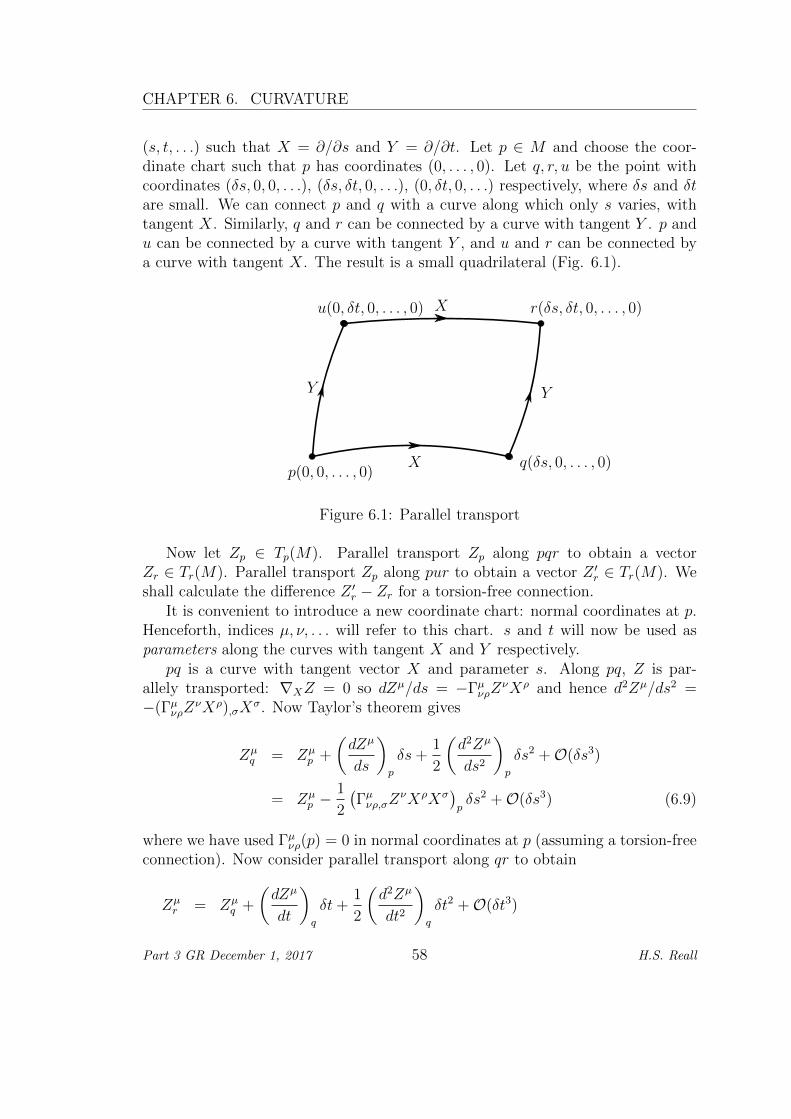
CHAPTER 6. CURVATURE
(s, t, . . .) such that X = ∂/∂s and Y = ∂/∂t. Let p ∈ M and choose the coor-dinate chart such that p has coordinates (0, . . . , 0). Let q, r, u be the point withcoordinates (δs, 0, 0, . . .), (δs, δt, 0, . . .), (0, δt, 0, . . .) respectively, where δs and δtare small. We can connect p and q with a curve along which only s varies, withtangent X. Similarly, q and r can be connected by a curve with tangent Y . p andu can be connected by a curve with tangent Y , and u and r can be connected bya curve with tangent X. The result is a small quadrilateral (Fig. 6.1).
X
X
Y Y
p(0, 0, . . . , 0)
u(0, δt, 0, . . . , 0)
q(δs, 0, . . . , 0)
r(δs, δt, 0, . . . , 0)
Figure 6.1: Parallel transport
Now let Zp ∈ Tp(M). Parallel transport Zp along pqr to obtain a vectorZr ∈ Tr(M). Parallel transport Zp along pur to obtain a vector Z ′r ∈ Tr(M). Weshall calculate the difference Z ′r − Zr for a torsion-free connection.
It is convenient to introduce a new coordinate chart: normal coordinates at p.Henceforth, indices µ, ν, . . . will refer to this chart. s and t will now be used asparameters along the curves with tangent X and Y respectively.
pq is a curve with tangent vector X and parameter s. Along pq, Z is par-allely transported: ∇XZ = 0 so dZµ/ds = −ΓµνρZ
νXρ and hence d2Zµ/ds2 =−(ΓµνρZ
νXρ),σXσ. Now Taylor’s theorem gives
Zµq = Zµ
p +
(dZµ
ds
)p
δs+1
2
(d2Zµ
ds2
)p
δs2 +O(δs3)
= Zµp −
1
2
(Γµνρ,σZ
νXρXσ)pδs2 +O(δs3) (6.9)
where we have used Γµνρ(p) = 0 in normal coordinates at p (assuming a torsion-freeconnection). Now consider parallel transport along qr to obtain
Zµr = Zµ
q +
(dZµ
dt
)q
δt+1
2
(d2Zµ
dt2
)q
δt2 +O(δt3)
Part 3 GR December 1, 2017 58 H.S. Reall
6.4. SYMMETRIES OF THE RIEMANN TENSOR
= Zµq −
(ΓµνρZ
νY ρ)qδt− 1
2
((ΓµνρZ
νY ρ),σYσ)qδt2 +O(δt3)
= Zµq −
[(Γµνρ,σZ
νY ρXσ)pδs+O(δs2)
]δt
−1
2
[((Γµνρ,σZ
νY ρY σ)p
+O(δs)]δt2 +O(δt3)
= Zµp −
1
2
(Γµνρ,σ
)p
[Zν(XρXσδs2 + Y ρY σδt2 + 2Y ρXσδsδt
)]p
+O(δ3)
(6.10)
Here we assume that δs and δt both are O(δ) (i.e. δs = aδ for some non-zeroconstant a and similarly for δt). Now consider parallel transport along pur. Theresult can be obtained from the above expression simply by interchanging X withY and s with t. Hence we have
∆Zµr ≡ Z
′µr − Zµ
r =[Γµνρ,σZ
ν (Y ρXσ −XρY σ)]pδsδt+O(δ3)
=[(
Γµνσ,ρ − Γµνρ,σ)ZνXρY σ
]pδsδt+O(δ3)
= (RµνρσZ
νXρY σ)p δsδt+O(δ3)
= (RµνρσZ
νXρY σ)r δsδt+O(δ3) (6.11)
where we used the expression (6.6) for the Riemann tensor components (rememberthat Γµνρ(p) = 0). In the final equality we used that quantities at p and r differby O(δ). We have derived this result in a coordinate basis defined using normalcoordinates at p. But now both sides involve tensors at r. Hence our equation isbasis-independent so we can write(
RabcdZ
bXcY d)r
= limδ→0
∆Zar
δsδt(6.12)
The Riemann tensor measures the path-dependence of parallel transport.
Remark. We considered parallel transport along two different curves from p to r.However, we can reinterpret the result as describing the effect of parallel transportof a vector Za
r around the closed curve rqpur to give the vector Z′ar . Hence ∆Za
r
measures the change in Zar when parallel transported around a closed curve.
6.4 Symmetries of the Riemann tensor
From its definition, we have the symmetry Rabcd = −Ra
bdc, equivalently:
Rab(cd) = 0. (6.13)
Proposition. If ∇ is torsion-free then
Part 3 GR December 1, 2017 59 H.S. Reall
CHAPTER 6. CURVATURE
Ra[bcd] = 0. (6.14)
Proof. Let p ∈ M and choose normal coordinates at p. Vanishing torsion impliesΓµνρ(p) = 0 and Γµ[νρ] = 0 everywhere. We have Rµ
νρσ = ∂ρΓµνσ − ∂σΓµνρ at p.
Antisymmetrizing on νρσ now gives Rµ[νρσ] = 0 at p in the coordinate basis defined
using normal coordinates at p. But if the components of a tensor vanish in onebasis then they vanish in any basis. This proves the result at p. However, p isarbitrary so the result holds everywhere.
Proposition. (Bianchi identity). If ∇ is torsion-free then
Rab[cd;e] = 0 (6.15)
Proof. Use normal coordinate at p again. At p,
Rµνρσ;τ = ∂τR
µνρσ (6.16)
In normal coordinates at p, ∂R = ∂∂Γ−Γ∂Γ and the latter terms vanish at p, weonly need to worry about the former:
Rµνρσ;τ = ∂τ∂ρΓ
µνσ − ∂τ∂σΓµνρ at p (6.17)
Antisymmetrizing gives Rµν[ρσ;τ ] = 0 at p in this basis. But again, if this is true
in one basis then it is true in any basis. Furthermore, p is arbitrary. The resultfollows.
6.5 Geodesic deviation
Remark. In Euclidean space, or in Minkowski spacetime, initially parallel geodesicsremain parallel forever. On a general manifold we have no notion of ”parallel”.However, we can study whether nearby geodesics move together or apart. In par-ticular, we can quantify their ”relative acceleration”.
Definition. Let M be a manifold with a connection ∇. A 1-parameter family ofgeodesics is a map γ : I × I ′ → M where I and I ′ both are open intervals in R,such that (i) for fixed s, γ(s, t) is a geodesic with affine parameter t (so s is theparameter that labels the geodesic); (ii) the map (s, t) 7→ γ(s, t) is smooth andone-to-one with a smooth inverse. This implies that the family of geodesics formsa 2d surface Σ ⊂M .
Let T be the tangent vector to the geodesics and S to be the vector tangentto the curves of constant t, which are parameterized by s (see Fig. 6.2). Ina chart xµ, the geodesics are specified by xµ(s, t) with Sµ = ∂xµ/∂s. Hence
Part 3 GR December 1, 2017 60 H.S. Reall
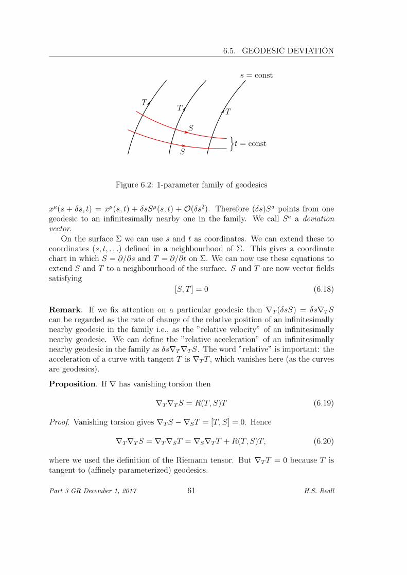
6.5. GEODESIC DEVIATION
t = const
S
S
TT T
s = const
Figure 6.2: 1-parameter family of geodesics
xµ(s + δs, t) = xµ(s, t) + δsSµ(s, t) + O(δs2). Therefore (δs)Sa points from onegeodesic to an infinitesimally nearby one in the family. We call Sa a deviationvector.
On the surface Σ we can use s and t as coordinates. We can extend these tocoordinates (s, t, . . .) defined in a neighbourhood of Σ. This gives a coordinatechart in which S = ∂/∂s and T = ∂/∂t on Σ. We can now use these equations toextend S and T to a neighbourhood of the surface. S and T are now vector fieldssatisfying
[S, T ] = 0 (6.18)
Remark. If we fix attention on a particular geodesic then ∇T (δsS) = δs∇TScan be regarded as the rate of change of the relative position of an infinitesimallynearby geodesic in the family i.e., as the ”relative velocity” of an infinitesimallynearby geodesic. We can define the ”relative acceleration” of an infinitesimallynearby geodesic in the family as δs∇T∇TS. The word ”relative” is important: theacceleration of a curve with tangent T is ∇TT , which vanishes here (as the curvesare geodesics).
Proposition. If ∇ has vanishing torsion then
∇T∇TS = R(T, S)T (6.19)
Proof. Vanishing torsion gives ∇TS −∇ST = [T, S] = 0. Hence
∇T∇TS = ∇T∇ST = ∇S∇TT +R(T, S)T, (6.20)
where we used the definition of the Riemann tensor. But ∇TT = 0 because T istangent to (affinely parameterized) geodesics.
Part 3 GR December 1, 2017 61 H.S. Reall
CHAPTER 6. CURVATURE
Remark. This result is known as the geodesic deviation equation. In abstractindex notation it is:
T c∇c(Tb∇bS
a) = RabcdT
bT cSd (6.21)
This equation shows that curvature results in relative acceleration of geodesics.It also provides another method of measuring Ra
bcd: at any point p we can pickour 1-parameter family of geodesics such that T and S are arbitrary. Hence bymeasuring the LHS above we can determine Ra
(bc)d. From this we can determineRa
bcd:
Exercise. Show that, for a torsion-free connection,
Rabcd =
2
3
(Ra
(bc)d −Ra(bd)c
)(6.22)
Remarks.
1. Note that the relative acceleration vanishes for all families of geodesics if,and only if, Ra
bcd = 0.
2. In GR, free particles follow geodesics of the Levi-Civita connection. Geodesicdeviation is the tendency of freely falling particles to move together or apart.We have already met this phenomenon: it arises from tidal forces. Hence theRiemann tensor is the quantity that measures tidal forces.
6.6 Curvature of the Levi-Civita connection
Remark. From now on, we shall restrict attention to a manifold with metric,and use the Levi-Civita connection. The Riemann tensor then enjoys additionalsymmetries. Note that we can lower an index with the metric to define Rabcd.
Proposition. The Riemann tensor satisfies
Rabcd = Rcdab, R(ab)cd = 0. (6.23)
Proof. The second identity follows from the first and the antisymmetry of theRiemann tensor. To prove the first, introduce normal coordinates at p, so ∂µgνρ = 0at p. Then, at p,
0 = ∂µδνρ = ∂µ (gνσgσρ) = gσρ∂µg
νσ. (6.24)
Multiplying by the inverse metric gives ∂µgνρ = 0 at p. Using this, we have
∂ρΓτνσ =
1
2gτµ (gµν,σρ + gµσ,νρ − gνσ,µρ) at p (6.25)
Part 3 GR December 1, 2017 62 H.S. Reall
6.7. EINSTEIN’S EQUATION
And hence (as Γµνρ = 0 at p)
Rµνρσ =1
2(gµσ,νρ + gνρ,µσ − gνσ,µρ − gµρ,νσ) at p (6.26)
This satisfies Rµνρσ = Rρσµν at p using the symmetry of the metric and the fact thatpartial derivatives commute. This establishes the identity in normal coordinates,but this is a tensor equation and hence valid in any basis. Furthermore p isarbitrary so the identity holds everywhere.
Proposition. The Ricci tensor is symmetric:
Rab = Rba (6.27)
Proof. Rab = gcdRdacb = gcdRcbda = Rcbca = Rba where we used the first identity
above in the second equality.
Definition. The Ricci scalar is
R = gabRab (6.28)
Definition. The Einstein tensor is the symmetric (0, 2) tensor defined by
Gab = Rab −1
2Rgab (6.29)
Proposition. The Einstein tensor satisfies the contracted Bianchi identity:
∇aGab = 0 (6.30)
which can also be written as
∇aRab −1
2∇bR = 0 (6.31)
Proof. Examples sheet 2.
6.7 Einstein’s equation
Postulates of General Relativity.
1. Spacetime is a 4d Lorentzian manifold equipped with the Levi-Civita con-nection.
2. Free particles follow timelike or null geodesics.
Part 3 GR December 1, 2017 63 H.S. Reall
CHAPTER 6. CURVATURE
3. The energy, momentum, and stresses of matter are described by a symmetrictensor Tab that is conserved: ∇aTab = 0.
4. The curvature of spacetime is related to the energy-momentum tensor ofmatter by the Einstein equation (1915)
Gab ≡ Rab −1
2Rgab = 8πGTab (6.32)
where G is Newton’s constant.
We have discussed points 1-3 above. It remains to discuss the Einstein equation.We can motivate this as follows. In GR, the gravitational field is described bythe curvature of spacetime. Since the energy of matter should be responsiblefor gravitation, we expect some relationship between curvature and the energy-momentum tensor. The simplest possibility is a linear relationship, i.e., a curvaturetensor is proportional to Tab. Since Tab is symmetric, it is natural to expect theRicci tensor to be the relevant curvature tensor.
Einstein’s first guess for the field equation of GR was Rab = CTab for someconstant C. This does not work for the following reason. The RHS is conservedhence this equation implies ∇aRab = 0. But then from the contracted Bianchiidentity we get ∇aR = 0. Taking the trace of the equation gives R = CT (whereT = T aa) and hence we must have ∇aT = 0, i.e., T is constant. But, T vanishesin empty space and is usually non-zero inside matter. Hence this is unsatisfactory.
The solution to this problem is obvious once one knows of the contractedBianchi identity. Take Gab, rather than Rab, to be proportional to Tab. The coeffi-cient of proportionality on the RHS of Einstein’s equation is fixed by demandingthat the equation reduces to Newton’s law of gravitation when the gravitationalfield is weak and the matter is moving non-relativistically. We will show this later.
Remarks.
1. In vacuum, Tab = 0 so Einstein’s equation gives Gab = 0. Contracting indicesgives R = 0. Hence the vacuum Einstein equation can be written as
Rab = 0 (6.33)
2. The ”geodesic postulate” of GR is redundant. Using conservation of theenergy-momentum tensor it can be shown that a distribution of matter thatis small (compared to the scale on which the spacetime metric varies), andsufficiently weak (so that its gravitational effect is small), must follow ageodesic. (See examples sheet 4 for the case of a point particle.)
Part 3 GR December 1, 2017 64 H.S. Reall
6.7. EINSTEIN’S EQUATION
3. The Einstein equation is a set of non-linear, second order, coupled, partialdifferential equations for the components of the metric gµν . Very few phys-ically interesting explicit solutions are known so one has to develop othermethods to solve the equation, e.g., numerical integration.
4. How unique is the Einstein equation? Is there any tensor, other than Gab
that we could have put on the LHS? The answer is supplied by:
Theorem (Lovelock 1972). Let Hab be a symmetric tensor such that (i) in anycoordinate chart, at any point, Hµν is a function of gµν , gµν,ρ and gµν,ρσ at thatpoint; (ii) ∇aHab = 0; (iii) either spacetime is four-dimensional or Hµν dependslinearly on gµν,ρσ. Then there exist constants α and β such that
Hab = αGab + βgab (6.34)
Hence (as Einstein realized) there is the freedom to add a constant multiple of gabto the LHS of Einstein’s equation, giving
Gab + Λgab = 8πGTab (6.35)
Λ is called the cosmological constant. This no longer reduces to Newtonian theoryfor slow motion in a weak field but the deviation from Newtonian theory is unob-servable if Λ is sufficiently small. Note that |Λ|−1/2 has the dimensions of length.The effects of Λ are negligible on lengths or times small compared to this quantity.Astronomical observations suggest that there is indeed a very small positive cos-mological constant: Λ−1/2 ∼ 109 light years, the same order of magnitude as thesize of the observable Universe. Hence the effects of the cosmological constant arenegligible except on cosmological length scales. Therefore we can set Λ = 0 unlesswe discuss cosmology.
Note that we can move the cosmological constant term to the RHS of theEinstein equation, and regard it as the energy-momentum tensor of a perfect fluidwith ρ = −p = Λ/(8πG). Hence the cosmological constant is sometimes referredto as dark energy or vacuum energy. It is a great mystery why it is so small becausearguments from quantum field theory suggest that it should be 10120 times larger.This is the cosmological constant problem. One (controversial) proposed solutionof this problem invokes the anthropic principle, which posits the existence of manypossible universes with different values for constants such as Λ. If Λ was verydifferent from its observed value then galaxies never would have formed and hencewe would not be here.
Remark. We have explicitly written Newton’s constant G throughout this section.Henceforth we shall choose units so that G = c = 1.
Part 3 GR December 1, 2017 65 H.S. Reall

CHAPTER 6. CURVATURE
Part 3 GR December 1, 2017 66 H.S. Reall
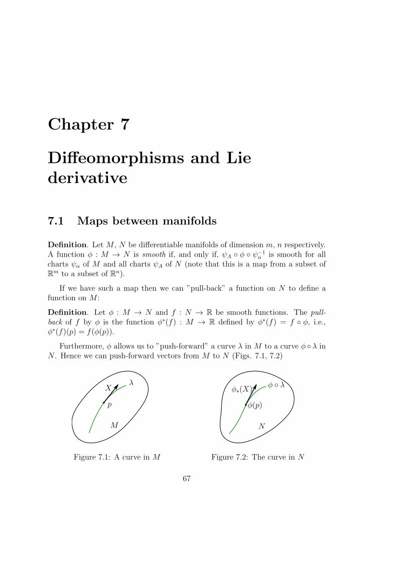
Chapter 7
Diffeomorphisms and Liederivative
7.1 Maps between manifolds
Definition. Let M , N be differentiable manifolds of dimension m, n respectively.A function φ : M → N is smooth if, and only if, ψA φ ψ−1
α is smooth for allcharts ψα of M and all charts ψA of N (note that this is a map from a subset ofRm to a subset of Rn).
If we have such a map then we can ”pull-back” a function on N to define afunction on M :
Definition. Let φ : M → N and f : N → R be smooth functions. The pull-back of f by φ is the function φ∗(f) : M → R defined by φ∗(f) = f φ, i.e.,φ∗(f)(p) = f(φ(p)).
Furthermore, φ allows us to ”push-forward” a curve λ in M to a curve φ λ inN . Hence we can push-forward vectors from M to N (Figs. 7.1, 7.2)
M
λX
p
Figure 7.1: A curve in M
N
φ λφ∗(X)
φ(p)
Figure 7.2: The curve in N
67
CHAPTER 7. DIFFEOMORPHISMS AND LIE DERIVATIVE
Definition. Let φ : M → N be smooth. Let p ∈ M and X ∈ Tp(M). Thepush-forward of X with respect to φ is the vector φ∗(X) ∈ Tφ(p)(N) defined asfollows. Let λ be a smooth curve in M passing through p with tangent X at p.Then φ∗(X) is the tangent vector to the curve φ λ in N at the point φ(p).
Lemma. Let f : N → R. Then (φ∗(X))(f) = X(φ∗(f)).Proof. Wlog λ(0) = p.
(φ∗(X))(f) =
[d
dt(f (φ λ))(t)
]t=0
=
[d
dt((f φ) λ)(t)
]t=0
= X(φ∗(f)) (7.1)
Exercise. Let xµ be coordinates on M and yα be coordinates on N (we usedifferent indices α, β etc for N because N is a different manifold which might nothave the same dimension as M). Then we can regard φ as defining a map yα(xµ).Show that the components of φ∗(X) are related to those of X by
(φ∗(X))α =
(∂yα
∂xµ
)p
Xµ (7.2)
The map on covectors works in the opposite direction:
Definition. Let φ : M → N be smooth. Let p ∈ M and η ∈ T ∗φ(p)(N). The pull-
back of η with respect to φ is φ∗(η) ∈ T ∗p (M) defined by (φ∗(η))(X) = η(φ∗(X))for any X ∈ Tp(M).
Lemma. Let f : N → R. Then φ∗(df) = d(φ∗(f)).Proof. Let X ∈ Tp(M). Then
(φ∗(df))(X) = (df)(φ∗(X)) = (φ∗(X))(f) = X(φ∗(f)) = (d(φ∗(f)))(X) (7.3)
The first equality is the definition of φ∗, the second is the definition of df , thethird is the previous Lemma and the fourth is the definition of d(φ∗(f)). Since Xis arbitrary, the result follows.
Exercise. Use coordinates xµ and yα as before. Show that the components ofφ∗(η) are related to the components of η by
(φ∗(η))µ =
(∂yα
∂xµ
)p
ηα (7.4)
Remarks.
Part 3 GR December 1, 2017 68 H.S. Reall
7.2. DIFFEOMORPHISMS, LIE DERIVATIVE
1. In all of the above, the point p was arbitrary so push-forward and pull-backcan be applied to vector and covector fields, respectively.
2. The pull-back can be extended to a tensor S of type (0, s) by defining(φ∗(S))(X1, . . . Xs) = S(φ∗(X1), . . . φ∗(Xs)) whereX1, . . . , Xs ∈ Tp(M). Sim-ilarly, one can push-forward a tensor of type (r, 0) by defining φ∗(T )(η1, . . . , ηr) =T (φ∗(η1), . . . , φ∗(ηr)) where η1, . . . , ηr ∈ T ∗p (N). The components of thesetensors in a coordinate basis are given by
(φ∗(S))µ1...µs =
(∂yα1
∂xµ1
)p
. . .
(∂yαs
∂xµs
)p
Sα1...αs (7.5)
(φ∗(T ))α1...αr =
(∂yα1
∂xµ1
)p
. . .
(∂yαr
∂xµr
)p
T µ1...µr (7.6)
Example. The embedding of S2 into Euclidean space. Let M = S2 and N =R3. Define φ : M → N as the map which sends the point on S2 with sphericalpolar coordinates xµ = (θ, φ) to the point yα = (sin θ cosφ, sin θ sinφ, cos θ) ∈ R3.Consider the Euclidean metric g on R3, whose components are the identity matrixδαβ. Pulling this back to S2 using (7.5) gives (φ∗g)µν = diag(1, sin2 θ) (check!), theunit round metric on S2.
7.2 Diffeomorphisms, Lie Derivative
Definition. A map φ : M → N is a diffeomorphism iff it 1-1 and onto, smooth,and has a smooth inverse.
Remark. This implies that M and N have the same dimension. In fact, M andN have identical manifold structure.
With a diffeomorphism, we can extend our definitions of push-forward andpull-back so that they apply for any type of tensor:
Definition. Let φ : M → N be a diffeomorphism and T a tensor of type (r, s) onM . Then the push-forward of T is a tensor φ∗(T ) of type (r, s) on N defined by(for arbitrary ηi ∈ T ∗φ(p)(N), Xi ∈ Tφ(p)(N))
φ∗(T )(η1, . . . , ηr, X1, . . . , Xs) = T (φ∗(η1), . . . , φ∗(ηr), (φ−1)∗(X1), . . . , (φ−1)∗(Xs))
(7.7)
Exercises.
1. Convince yourself that push-forward commutes with the contraction andouter product operations.
Part 3 GR December 1, 2017 69 H.S. Reall
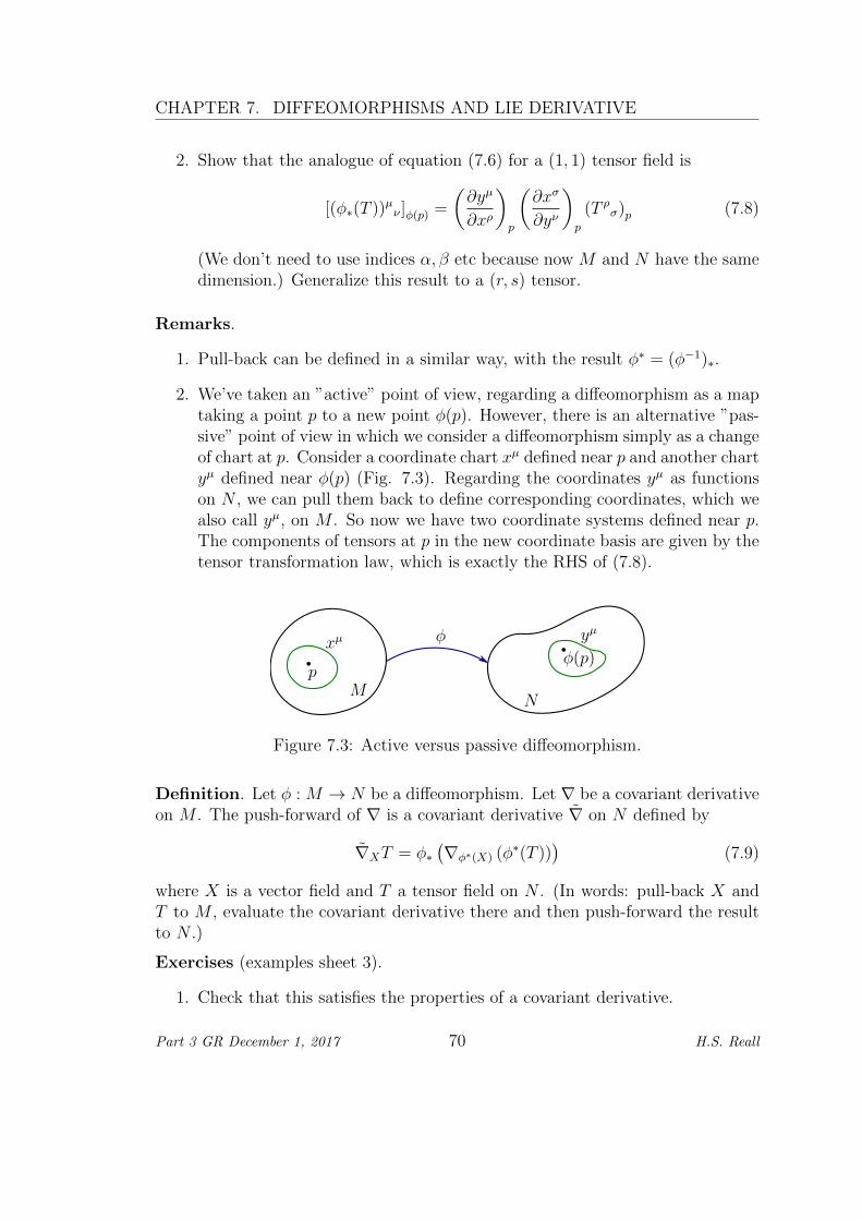
CHAPTER 7. DIFFEOMORPHISMS AND LIE DERIVATIVE
2. Show that the analogue of equation (7.6) for a (1, 1) tensor field is
[(φ∗(T ))µν ]φ(p) =
(∂yµ
∂xρ
)p
(∂xσ
∂yν
)p
(T ρσ)p (7.8)
(We don’t need to use indices α, β etc because now M and N have the samedimension.) Generalize this result to a (r, s) tensor.
Remarks.
1. Pull-back can be defined in a similar way, with the result φ∗ = (φ−1)∗.
2. We’ve taken an ”active” point of view, regarding a diffeomorphism as a maptaking a point p to a new point φ(p). However, there is an alternative ”pas-sive” point of view in which we consider a diffeomorphism simply as a changeof chart at p. Consider a coordinate chart xµ defined near p and another chartyµ defined near φ(p) (Fig. 7.3). Regarding the coordinates yµ as functionson N , we can pull them back to define corresponding coordinates, which wealso call yµ, on M . So now we have two coordinate systems defined near p.The components of tensors at p in the new coordinate basis are given by thetensor transformation law, which is exactly the RHS of (7.8).
p
xµφ(p)
yµφ
MN
Figure 7.3: Active versus passive diffeomorphism.
Definition. Let φ : M → N be a diffeomorphism. Let ∇ be a covariant derivativeon M . The push-forward of ∇ is a covariant derivative ∇ on N defined by
∇XT = φ∗(∇φ∗(X) (φ∗(T ))
)(7.9)
where X is a vector field and T a tensor field on N . (In words: pull-back X andT to M , evaluate the covariant derivative there and then push-forward the resultto N .)
Exercises (examples sheet 3).
1. Check that this satisfies the properties of a covariant derivative.
Part 3 GR December 1, 2017 70 H.S. Reall
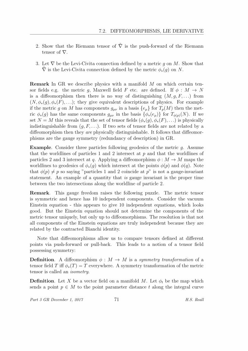
7.2. DIFFEOMORPHISMS, LIE DERIVATIVE
2. Show that the Riemann tensor of ∇ is the push-forward of the Riemanntensor of ∇.
3. Let ∇ be the Levi-Civita connection defined by a metric g on M . Show that∇ is the Levi-Civita connection defined by the metric φ∗(g) on N .
Remark In GR we describe physics with a manifold M on which certain ten-sor fields e.g. the metric g, Maxwell field F etc. are defined. If φ : M → Nis a diffeomorphism then there is no way of distinguishing (M, g, F, . . .) from(N, φ∗(g), φ∗(F ), . . .); they give equivalent descriptions of physics. For exampleif the metric g on M has components gµν in a basis eµ for Tp(M) then the met-ric φ∗(g) has the same components gµν in the basis φ∗(eµ) for Tφ(p)(N). If weset N = M this reveals that the set of tensor fields (φ∗(g), φ∗(F ), . . .) is physicallyindistinguishable from (g, F, . . .). If two sets of tensor fields are not related by adiffeomorphism then they are physically distinguishable. It follows that diffeomor-phisms are the gauge symmetry (redundancy of description) in GR.
Example. Consider three particles following geodesics of the metric g. Assumethat the worldlines of particles 1 and 2 intersect at p and that the worldlines ofparticles 2 and 3 intersect at q. Applying a diffeomorphism φ : M →M maps theworldlines to geodesics of φ∗(g) which intersect at the points φ(p) and φ(q). Notethat φ(p) 6= p so saying ”particles 1 and 2 coincide at p” is not a gauge-invariantstatement. An example of a quantity that is gauge invariant is the proper timebetween the two intersections along the worldline of particle 2.
Remark. This gauge freedom raises the following puzzle. The metric tensoris symmetric and hence has 10 independent components. Consider the vacuumEinstein equation - this appears to give 10 independent equations, which looksgood. But the Einstein equation should not determine the components of themetric tensor uniquely, but only up to diffeomorphisms. The resolution is that notall components of the Einstein equations are truly independent because they arerelated by the contracted Bianchi identity.
Note that diffeomorphisms allow us to compare tensors defined at differentpoints via push-forward or pull-back. This leads to a notion of a tensor fieldpossessing symmetry:
Definition. A diffeomorphism φ : M → M is a symmetry transformation of atensor field T iff φ∗(T ) = T everywhere. A symmetry transformation of the metrictensor is called an isometry.
Definition. Let X be a vector field on a manifold M . Let φt be the map whichsends a point p ∈ M to the point parameter distance t along the integral curve
Part 3 GR December 1, 2017 71 H.S. Reall
CHAPTER 7. DIFFEOMORPHISMS AND LIE DERIVATIVE
of X through p (this might be defined only for small enough t). It can be shownthat φt is a diffeomorphism.
Remarks.
1. Note that φ0 is the identity map and φs φt = φs+t. Hence φ−t = (φt)−1. If
φt is defined for all t ∈ R (in which case we say the integral curves of X arecomplete) then these diffeomorphisms form a 1-parameter abelian group.
2. Given X we’ve defined φt. Conversely, if one has a 1-parameter abeliangroup of diffeomorphisms φt (i.e. one satisfying the rules just mentioned)then through any point p one can consider the curve with parameter t givenby φt(p). Define X to be the tangent to this curve at p. Doing this for allp defines a vector field X. The integral curves of X generate φt in the sensedefined above.
3. If we use (φt)∗ to compare tensors at different points then the parameter tcontrols how near the points are. In particular, in the limit t → 0, we arecomparing tensors at infinitesimally nearby points. This leads to the notionof a new type of derivative:
Definition. The Lie derivative of a tensor field T with respect to a vector fieldX at p is
(LXT )p = limt→0
((φ−t)∗T )p − Tpt
(7.10)
Remark. The Lie derivative wrt X is a map from (r, s) tensor fields to (r, s) tensor
fields. It obeys LX(αS + βT ) = αLXS + βLXT where α and β are constants.
The easiest way to demonstrate other properties of the Lie derivative is tointroduce coordinates in which the components of X are simple. Let Σ be ahypersurface that has the property that X is nowhere tangent to Σ (in particularX 6= 0 on Σ). Let xi, i = 1, 2, . . . , n − 1 be coordinates on Σ. Now assigncoordinates (t, xi) to the point parameter distance t along the integral curve of Xthat starts at the point with coordinates xi on Σ (Fig. 7.4).
This defines a coordinate chart (t, xi) at least for small t, i.e., in a neighbour-hood of Σ. Furthermore, the integral curves of X are the curves (t, xi) with fixedxi and parameter t. The tangent to these curves is ∂/∂t so we have constructedcoordinates such that X = ∂/∂t. The diffeomorphism φt is very simple: it justsends the point p with coordinates xµ = (tp, x
ip) to the point φt(p) with coordinates
yµ = (tp + t, xip) hence ∂yµ/∂xν = δµν . The generalization of (7.8) to a (r, s) tensorthen gives
[((φ−t)∗(T ))µ1,...,µrν1,...νs ]φ−t(q) = [T µ1,...,µrν1,...νs ]q (7.11)
Part 3 GR December 1, 2017 72 H.S. Reall
7.2. DIFFEOMORPHISMS, LIE DERIVATIVE
Σ
xi
(t, xi)
X
Figure 7.4: Coordinates adapted to a vector field
and setting q = φt(p) gives
[((φ−t)∗(T ))µ1,...,µrν1,...νs ]p = [T µ1,...,µrν1,...νs ]φt(p) (7.12)
It follows that, if p has coordinates (tp, xip) in this chart,
(LXT )µ1,...,µrν1,...νs = limt→0
1
t
[T µ1,...,µrν1,...νs(tp + t, xip)− T µ1,...,µrν1,...νs(tp, xip)
]=
(∂
∂tT µ1,...,µrν1,...νs
)(tp, x
ip) (7.13)
So in this chart, the Lie derivative is simply the partial derivative with respect tothe coordinate t. It follows that the Lie derivative has the following properties:
1. It obeys the Leibniz rule: LX(S ⊗ T ) = (LXS)⊗ T + S ⊗ LXT .
2. It commutes with contraction.
Now let’s derive a basis-independent formula for the Lie derivative. First con-sider a function f . In the above chart, we have LXf = (∂/∂t)(f). However, inthis chart we also have X(f) = (∂/∂t)(f). Hence
LXf = X(f) (7.14)
Both sides of this expression are scalars and hence this equation must be valid inany basis. Next consider a vector field Y . In our coordinates above we have
(LXY )µ =∂Y µ
∂t(7.15)
but we also have
[X, Y ]µ =∂Y µ
∂t(7.16)
Part 3 GR December 1, 2017 73 H.S. Reall
CHAPTER 7. DIFFEOMORPHISMS AND LIE DERIVATIVE
If two vectors have the same components in one basis then they are equal in allbases. Hence we have the basis-independent result
LXY = [X, Y ] (7.17)
Remark. Let’s compare the Lie derivative and the covariant derivative. The
former is defined on any manifold whereas the latter requires extra structure (aconnection). Equation (7.17) reveals that the Lie derivative wrt X at p dependson Xp and the first derivatives of X at p. The covariant derivative wrt X at pdepends only on Xp, which enables us to remove X to define the tensor ∇T , acovariant generalization of partial differentiation. It is not possible to define acorresponding tensor LT using the Lie derivative. Only LXT makes sense.
Exercises (examples sheet 3).
1. Derive the formula for the Lie derivative of a covector ω in a coordinatebasis:
(LXω)µ = Xν∂νωµ + ων∂µXν (7.18)
Show that this can be written in the basis-independent form (where ∇ is theLevi-Civita connection)
(LXω)a = Xb∇bωa + ωb∇aXb (7.19)
2. Show that the Lie derivative of the metric in a coordinate basis is
(LXg)µν = Xρ∂ρgµν + gµρ∂νXρ + gρν∂µX
ρ (7.20)
and that this can be written in the basis-independent form
(LXg)ab = ∇aXb +∇bXa (7.21)
Remark. If φt is a symmetry transformation of T (for all t) then LXT = 0. If φtare a 1-parameter group of isometries then LXg = 0, i.e.,
∇aXb +∇bXa = 0 (7.22)
This is Killing’s equation and solutions are called Killing vector fields. Considerthe case in which there exists a chart for which the metric tensor does not de-pend on some coordinate z. Then equation (7.20) reveals that ∂/∂z is a Killingvector field. Conversely, if the metric admits a Killing vector field then equation(7.13) demonstrates that one can introduce coordinates such that the metric tensorcomponents are independent of one of the coordinates.
Part 3 GR December 1, 2017 74 H.S. Reall
7.2. DIFFEOMORPHISMS, LIE DERIVATIVE
Lemma. Let Xa be a Killing vector field and let V a be tangent to an affinelyparameterized geodesic. Then XaV
a is constant along the geodesic.Proof. The derivative of XaV
a along the geodesic is
d
dτ(XaV
a) = V (XaVa) = ∇V (XaV
a) = V b∇b(XaVa)
= V aV b∇bXa +XaVb∇bV
a (7.23)
The first term vanishes because Killing’s equation implies that ∇bXa is antisym-metric. The second term vanishes by the geodesic equation.
Exercise. Let Ja = T abXb where Tab is the energy-momentum tensor and Xb is
a Killing vector field. Show that ∇aJa = 0, i.e., Ja is a conserved current.
Part 3 GR December 1, 2017 75 H.S. Reall
CHAPTER 7. DIFFEOMORPHISMS AND LIE DERIVATIVE
Part 3 GR December 1, 2017 76 H.S. Reall
Chapter 8
Linearized theory
8.1 The linearized Einstein equation
The nonlinearity of the Einstein equation makes it very hard to solve. However,in many circumstances, gravity is not strong and spacetime can be regarded asa perturbation of Minkowski spacetime. More precisely, we assume our space-time manifold is M = R4 and that there exist globally defined ”almost inertial”coordinates xµ for which the metric can be written
gµν = ηµν + hµν , ηµν = diag(−1, 1, 1, 1) (8.1)
with the weakness of the gravitational field corresponding to the components ofhµν being small compared to 1. Note that we are dealing with a situation in whichwe have two metrics defined on spacetime, namely gab and the Minkowski metricηab. The former is supposed to be the physical metric, i.e., free particles move ongeodesics of gab.
In linearized theory we regard hµν as the components of a tensor field in thesense of special relativity, i.e., it transforms as a tensor under Lorentz transforma-tions of the coordinates xµ.
To leading order in the perturbation, the inverse metric is
gµν = ηµν − hµν , (8.2)
where we definehµν = ηµρηνσhρσ (8.3)
To prove this, just check that gµνgνρ = δµρ to linear order in the perturbation.Here, and henceforth, we shall raise and lower indices using the Minkowski metricηµν . To leading order this agrees with raising and lowering with gµν . We shalldetermine the Einstein equation to first order in the perturbation hµν .
77
CHAPTER 8. LINEARIZED THEORY
To first order, the Christoffel symbols are
Γµνρ =1
2ηµσ (hσν,ρ + hσρ,ν − hνρ,σ) , (8.4)
the Riemann tensor is (neglecting ΓΓ terms since they are second order in theperturbation):
Rµνρσ = ηµτ(∂ρΓ
τνσ − ∂σΓτνρ
)=
1
2(hµσ,νρ + hνρ,µσ − hνσ,µρ − hµρ,νσ) (8.5)
and the Ricci tensor is
Rµν = ∂ρ∂(µhν)ρ −1
2∂ρ∂ρhµν −
1
2∂µ∂νh, (8.6)
where ∂µ denotes ∂/∂xµ as usual, and
h = hµµ (8.7)
To first order, the Einstein tensor is
Gµν = ∂ρ∂(µhν)ρ −1
2∂ρ∂ρhµν −
1
2∂µ∂νh−
1
2ηµν (∂ρ∂σhρσ − ∂ρ∂ρh) . (8.8)
The Einstein equation equates this to 8πTµν (which must therefore be assumed tobe small, otherwise spacetime would not be nearly flat). It is convenient to define
hµν = hµν −1
2hηµν , (8.9)
with inverse
hµν = hµν −1
2hηµν , (h = hµµ = −h) (8.10)
The linearized Einstein equation is then (exercise)
−1
2∂ρ∂ρhµν + ∂ρ∂(µhν)ρ −
1
2ηµν∂
ρ∂σhρσ = 8πTµν (8.11)
We must now discuss the gauge symmetry present in this theory. We argued abovethat diffeomorphisms are gauge transformations in GR. A manifold M with metricg and energy-momentum tensor T is physically equivalent to M with metric φ∗(g)and energy momentum tensor φ∗(T ) if φ is a diffeomorphism. Now we are restrict-ing attention to metrics of the form (8.1). Hence we must consider which diffeo-morphisms preserve this form. A general diffeomorphism would lead to (φ∗(η))µνvery different from diag(−1, 1, 1, 1) and hence such a diffeomorphism would not
Part 3 GR December 1, 2017 78 H.S. Reall
8.1. THE LINEARIZED EINSTEIN EQUATION
preserve (8.1). However, if we consider a 1-parameter family of diffeomorphismsφt then φ0 is the identity map, so if t is small then φt is close to the identity andhence will have a small effect, i.e., (φt∗(η))µν will be close to diag(−1, 1, 1, 1) andthe form (8.1) will be preserved. For small t, we can use the definition of the Liederivative to deduce that, for any tensor T
(φ−t)∗(T ) = T + tLXT +O(t2)
= T + LξT +O(t2) (8.12)
where Xa is the vector field that generates φt and ξa = tXa. Note that ξa issmall so we treat it as a first order quantity. If we apply this result to the energy-momentum tensor, evaluating in our chart xµ, then the first term is small (byassumption) so the second term is higher order and can be neglected. Hence theenergy-momentum tensor is gauge-invariant to first order. The same is true forany tensor that vanishes in the unperturbed spacetime, e.g. the Riemann tensor.However, for the metric we have
(φ−t)∗(g) = g + Lξg + . . . = η + h+ Lξη + . . . (8.13)
where we have neglected Lξh because this is a higher order quantity (as ξ and hboth are small). Comparing this with (8.1) we deduce that h and h+Lξη describephysically equivalent metric perturbations. Therefore linearized GR has the gaugesymmetry h → h + Lξη for small ξµ. In our chart xµ, we can use (7.21) to write(Lξη)µν = ∂µξν + ∂νξµ and so the gauge symmetry is
hµν → hµν + ∂µξν + ∂νξµ (8.14)
There is a close analogy with electromagnetism in flat spacetime, where we canintroduce an electromagnetic potential Aµ, a 4-vector obeying Fµν = 2∂[µAν]. Thishas the gauge symmetry
Aµ → Aµ + ∂µΛ (8.15)
for some scalar Λ. In this case, one can choose Λ to impose the gauge condition∂µAµ = 0. Similarly, in linearized GR we can choose ξµ to impose the gaugecondition
∂ν hµν = 0. (8.16)
To see this, note that under the gauge transformation (8.14) we have
∂ν hµν → ∂ν hµν + ∂ν∂νξµ (8.17)
so if we choose ξµ to satisfy the wave equation ∂ν∂νξµ = −∂ν hµν (which we cansolve using a Green function) then we reach the gauge (8.16). This is called
Part 3 GR December 1, 2017 79 H.S. Reall
CHAPTER 8. LINEARIZED THEORY
variously Lorenz, de Donder, or harmonic gauge. In this gauge, the linearizedEinstein equation reduces to
∂ρ∂ρhµν = −16πTµν (8.18)
Hence, in this gauge, each component of hµν satisfies the wave equation witha source given by the energy-momentum tensor. Given appropriate boundaryconditions, the solution can be determined using a Green function.
8.2 The Newtonian limit
We will now see how GR reduces to Newtonian theory in the limit of non-relativisticmotion and a weak gravitational field. To do this, we could reintroduce factors ofc and try to expand everything in powers of 1/c since we expect Newtonian theoryto be valid as c→∞. We will follow an equivalent approach in which we stick toour convention c = 1 but introduce a small dimensionless parameter 0 < ε 1such that a factor of ε appears everywhere that a factor of 1/c would appear.
We assume that, for some choice of almost-inertial coordinates xµ = (t, xi), the3-velocity of any particle vi = dxi/dτ is O(ε). Recall that in Newtonian theory wehad v2 ∼ |Φ| (Fig. 1.1) and so we expect the gravitational field to be O(ε2). Weassume that
h00 = O(ε2), h0i = O(ε3), hij = O(ε2) (8.19)
We’ll see below how the additional factor of ε in h0i emerges.Since the matter which generates the gravitational field is assumed to move non-
relativistically, time derivatives of the gravitational field will be small compared tospatial derivatives. Let L denote the length scale over which hµν varies, i.e., if Xdenotes some component of hµν then |∂iX| = O(X/L). Our assumption of smalltime derivatives is
∂0X = O(εX/L) (8.20)
For example, in Newtonian theory, the gravitational field of a body of mass M atposition x(t) is Φ = −M/|x−x(t)| which obeys these formulae with L = |x−x(t)|and |x| = O(ε).
Consider the equations for a timelike geodesic. The Lagrangian is (adding ahat to avoid confusion with the length L)
L = (1− h00)t2 − 2h0itxi − (δij + hij) x
ixj (8.21)
where a dot denotes a derivative with respect to proper time τ . Our non-relativisticassumption implies that xi = O(ε). From the definition of proper time we haveL = 1 and hence
(1− h00)t2 − δijxixj = 1 +O(ε4) (8.22)
Part 3 GR December 1, 2017 80 H.S. Reall
8.2. THE NEWTONIAN LIMIT
Rearranging gives
t = 1 +1
2h00 +
1
2δijx
ixj +O(ε4) (8.23)
The Euler-Lagrange equation for xi is
d
dτ
[−2h0it− 2 (δij + hij) x
j]
= −h00,it2 − 2h0j,itx
j − hjk,ixjxk
= −h00,i +O(ε4/L) (8.24)
The LHS is −2xi plus subleading terms. Retaining only the leading order termsgives
xi =1
2h00,i (8.25)
Finally we can convert τ derivatives on the LHS to t derivatives using the chainrule and (8.23) to obtain
d2xi
dt2= −∂iΦ (8.26)
where
Φ ≡ −1
2h00 (8.27)
We have recovered the equation of motion for a test body moving in a Newtoniangravitational field Φ. Note that the weak equivalence principle automatically issatisfied: it follows from the fact that test bodies move on geodesics.
Exercise. Show that the corrections to (8.26) are O(ε4/L). You can argue asfollows. (8.25) implies xi = O(ε2/L). Now use (8.23) to show t = O(ε3/L).Expand out the derivative on the LHS of (8.24) to show that the corrections to(8.25) are O(ε4/L). Finally convert τ derivatives to t derivatives using (8.23).
The next thing we need to show is that Φ satisfies the Poisson equation (1.1).First consider the energy-momentum tensor. Assume that one can ascribe a 4-velocity ua to the matter. Our non-relativistic assumption implies
ui = O(ε), u0 = 1 +O(ε2) (8.28)
where the second equality follows from gabuaub = −1. The energy-density in the
rest-frame of the matter isρ ≡ uaubTab (8.29)
Recall that −T0i is the momentum density measured by an observer at rest in thesecoordinates so we expect −T0i ∼ ρui = O(ρε). Tij will have a part ∼ ρuiuj =O(ρε2) arising from the motion of the matter. It will also have a contributionfrom the stresses in the matter. Under all but the most extreme circumstances,
Part 3 GR December 1, 2017 81 H.S. Reall
CHAPTER 8. LINEARIZED THEORY
these are small compared to ρ. For example, in the rest frame of a perfect fluid,stresses are determined by the pressure p. The speed of sound in the fluid is Cwhere C2 = dp/dρ ∼ p/ρ. Our non-relativistic assumption is that C = O(ε) hencep = O(ρε2). This is true in the Solar system, where p/ρ ∼ |Φ| ∼ 10−5 at the centreof the Sun. Hence we make the following assumptions
T00 = ρ(1 +O(ε2)), T0i = O(ρε), Tij = O(ρε2) (8.30)
where the first equality follows from (8.29) and other two equalities.Finally, we consider the linearized Einstein equation. Equation (8.19) implies
thath00 = O(ε2), h0i = O(ε3), hij = O(ε2) (8.31)
Using our assumption about time derivatives being small compared to spatialderivatives, equation (8.18) becomes
∇2h00 = −16πρ(1 +O(ε2)), ∇2h0i = O(ρε), ∇2hij = O(ρε2) (8.32)
If we impose boundary conditions that the metric perturbation (gravitational field)should decay at large distance then these equations can be solved using a Greenfunction as in (1.2). The factors of ε on the RHS above imply that the resultingsolutions satisfy
h0i = O(h00ε) = O(ε3), hij = O(h00ε2) = O(ε4) (8.33)
Since h0i = h0i, this explains why we had to assume h0i = O(ε3). From the secondresult, we have hii = O(ε4) and hence h = −h00 + O(ε4). We can use (8.10) torecover hµν . This gives h00 = (1/2)h00 + O(ε4) and so, using (8.27) we obtainNewton’s law of gravitation:
∇2Φ = 4πρ(1 +O(ε2)) (8.34)
We also obtain hij = (1/2)h00δij +O(ε4) and so
hij = −2Φδij +O(ε4) (8.35)
This justifies the metric used in (1.16). The expansion of various quantities inpowers of ε can be extended to higher orders. As we have seen, the Newtonian ap-proximation requires only the O(ε2) term in h00. The next order, post-Newtonian,approximation corresponds to including O(ε4) terms in h00, O(ε3) terms in h0i andO(ε2) in hij. Equation (8.35) gives hij to O(ε2). The above analysis also lets uswrite the O(ε3) term in h0i in terms of T0i and a Green function. However, toobtain the O(ε4) term in h00 one has to go beyond linearized theory.
Part 3 GR December 1, 2017 82 H.S. Reall
8.3. GRAVITATIONAL WAVES
8.3 Gravitational waves
In vacuum, the linearized Einstein equation reduces to the source-free wave equa-tion:
∂ρ∂ρhµν = 0 (8.36)
so the theory admits gravitational wave solutions. As usual for the wave equation,we can build a general solution as a superposition of plane wave solutions. So let’slook for a plane wave solution:
hµν(x) = Re(Hµνe
ikρxρ)
(8.37)
where Hµν is a constant symmetric complex matrix describing the polarizationof the wave and kµ is the (real) wavevector. We shall suppress the Re in allsubsequent equations. The wave equation reduces to
kµkµ = 0 (8.38)
so the wavevector kµ must be null hence these waves propagate at the speed oflight relative to the background Minkowski metric. The gauge condition (8.16)gives
kνHµν = 0, (8.39)
i.e. the waves are transverse.
Example. Consider the null vector kµ = ω(1, 0, 0, 1). Then exp(ikµxµ) = exp(−iω(t−
z)) so this describes a wave of frequency ω propagating at the speed of light in thez-direction. The transverse condition reduces to
Hµ0 +Hµ3 = 0. (8.40)
Returning to the general case, the condition (8.16) does not eliminate all gaugefreedom. Consider a gauge transformation (8.14). From equation (8.17), we seethat this preserves the gauge condition (8.16) if ξµ obeys the wave equation:
∂ν∂νξµ = 0. (8.41)
Hence there is a residual gauge freedom which we can exploit to simplify thesolution. Take
ξµ(x) = Xµeikρxρ (8.42)
which satisfies (8.41) because kµ is null. Using
hµν → hµν + ∂µξν + ∂νξµ − ηµν∂ρξρ (8.43)
Part 3 GR December 1, 2017 83 H.S. Reall
CHAPTER 8. LINEARIZED THEORY
we see that the residual gauge freedom in our case is
Hµν → Hµν + i (kµXν + kνXµ − ηµνkρXρ) (8.44)
Exercise. Show that the residual gauge freedom can be used to achieve ”longitu-
dinal gauge”:H0µ = 0 (8.45)
but this still does not determine Xµ uniquely, and the freedom remains to imposethe additional ”trace-free” condition
Hµµ = 0. (8.46)
In this gauge, we havehµν = hµν . (8.47)
Example. Return to our wave travelling in the z-direction. The longitudinalgauge condition combined with the transversality condition (8.40) gives H3µ = 0.Using the trace-free condition now gives
Hµν =
0 0 0 00 H+ H× 00 H× −H+ 00 0 0 0
(8.48)
where the solution is specified by the two constants H+ and H× correspondingto two independent polarizations. So gravitational waves are transverse and havetwo possible polarizations. This is one way of interpreting the statement that thegravitational field has two degrees of freedom per spacetime point.
How would one detect a gravitational wave? An observer could set up a fam-ily of test particles locally. The displacement vector Sa from the observer to anyparticle is governed by the geodesic deviation equation. (We are taking Sa to beinfinitesimal, i.e., what we called δsSa previously.) So we can use this equationto predict what the observer would see. We have to be careful here. It would benatural to write out the geodesic deviation equation using the almost inertial co-ordinates and therby determine Sµ. But how would we relate this to observations?Sµ are the components of Sa with respect to a certain basis, so how would we de-termine whether the variation in Sµ arises from variation of Sa or from variationof the basis? With a bit more thought, one can make this approach work but weshall take a different approach.
Consider an observer following a geodesic in a general spacetime. Our observerwill be equipped with a set of measuring rods with which to measure distances.
Part 3 GR December 1, 2017 84 H.S. Reall
8.3. GRAVITATIONAL WAVES
At some point p on his worldline we could introduce a local inertial frame withspatial coordinates X, Y, Z in which the observer is at rest. Imagine that theobserver sets up measuring rods of unit length pointing in the X, Y, Z directionsat p. Mathematically, this defines an orthonormal basis eα for Tp(M) (we use αto label the basis vectors because we are using µ for our almost inertial coordinates)where ea0 = ua (his 4-velocity) and eai (i = 1, 2, 3) are spacelike vectors satisfying
uaeai = 0, gabe
ai ebj = δij (8.49)
In Minkowski spacetime, this basis can be extended to the observer’s entire world-line by taking the basis vectors to have constant components (in an inertial frame),i.e., they do not depend on proper time τ . In particular, this implies that the or-thonormal basis is non-rotating. Since the basis vectors have constant components,they are parallelly transported along the worldline. Hence, in curved spacetime,the analogue of this is to take the basis vectors to be parallelly transported alongthe worldline. For ua, this is automatic (the worldline is a geodesic). But for ei itgives
ub∇beai = 0 (8.50)
As we discussed previously, if the eai are specified at any point p then this equationdetermines them uniquely along the whole worldline. Furthermore, the basis re-mains orthonormal because parallel transport preserves inner products (examplessheet 2). The basis just constructed is sometimes called a parallelly transportedframe. It is the kind of basis that would be constructed by an observer freely fallingwith 3 gyroscopes whose spin axes define the spatial basis vectors. Using such abasis we can be sure that an increase in a component of Sa is really an increase inthe distance to the particle in a particular direction, rather than a basis-dependenteffect.
Now imagine this observer sets up a family of test particles near his worldline.The deviation vector to any infinitesimally nearby particle satisfies the geodesicdeviation equation
ub∇b(uc∇cSa) = Rabcdu
bucSd (8.51)
Contract with eaα and use the fact that the basis is parallelly transported to obtain
ub∇b[uc∇c(e
aαSa)] = Rabcde
aαu
bucSd (8.52)
Now eaαSa is a scalar hence the equation reduces to
d2Sαdτ 2
= Rabcdeaαu
bucedβSβ (8.53)
where τ is the observer’s proper time and Sα = eaαSa is one of the components ofSa in the parallelly transported frame. On the RHS we’ve used Sd = edβS
β.
Part 3 GR December 1, 2017 85 H.S. Reall
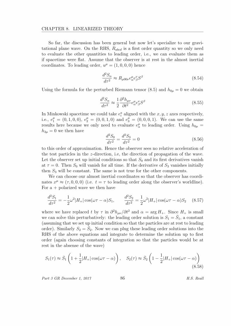
CHAPTER 8. LINEARIZED THEORY
So far, the discussion has been general but now let’s specialize to our gravi-tational plane wave. On the RHS, Rabcd is a first order quantity so we only needto evaluate the other quantities to leading order, i.e., we can evaluate them asif spacetime were flat. Assume that the observer is at rest in the almost inertialcoordinates. To leading order, uµ = (1, 0, 0, 0) hence
d2Sαdτ 2
≈ Rµ00νeµαe
νβS
β (8.54)
Using the formula for the perturbed Riemann tensor (8.5) and h0µ = 0 we obtain
d2Sαdτ 2
≈ 1
2
∂2hµν∂t2
eµαeνβS
β (8.55)
In Minkowski spacetime we could take eai aligned with the x, y, z axes respectively,i.e., eµ1 = (0, 1, 0, 0), eµ2 = (0, 0, 1, 0) and eµ3 = (0, 0, 0, 1). We can use the sameresults here because we only need to evaluate eµα to leading order. Using h0µ =h3µ = 0 we then have
d2S0
dτ 2=d2S3
dτ 2= 0 (8.56)
to this order of approximation. Hence the observer sees no relative acceleration ofthe test particles in the z-direction, i.e, the direction of propagation of the wave.Let the observer set up initial conditions so that S0 and its first derivatives vanishat τ = 0. Then S0 will vanish for all time. If the derivative of S3 vanishes initiallythen S3 will be constant. The same is not true for the other components.
We can choose our almost inertial coordinates so that the observer has coordi-nates xµ ≈ (τ, 0, 0, 0) (i.e. t = τ to leading order along the observer’s worldline).For a + polarized wave we then have
d2S1
dτ 2= −1
2ω2|H+| cos(ωτ − α)S1,
d2S2
dτ 2=
1
2ω2|H+| cos(ωτ − α)S2 (8.57)
where we have replaced t by τ in ∂2hµν/∂t2 and α = argH+. Since H+ is small
we can solve this perturbatively: the leading order solution is S1 = S1, a constant(assuming that we set up initial condition so that the particles are at rest to leadingorder). Similarly S2 = S2. Now we can plug these leading order solutions into theRHS of the above equations and integrate to determine the solution up to firstorder (again choosing constants of integration so that the particles would be atrest in the absense of the wave)
S1(τ) ≈ S1
(1 +
1
2|H+| cos(ωτ − α)
), S2(τ) ≈ S2
(1− 1
2|H+| cos(ωτ − α)
)(8.58)
Part 3 GR December 1, 2017 86 H.S. Reall
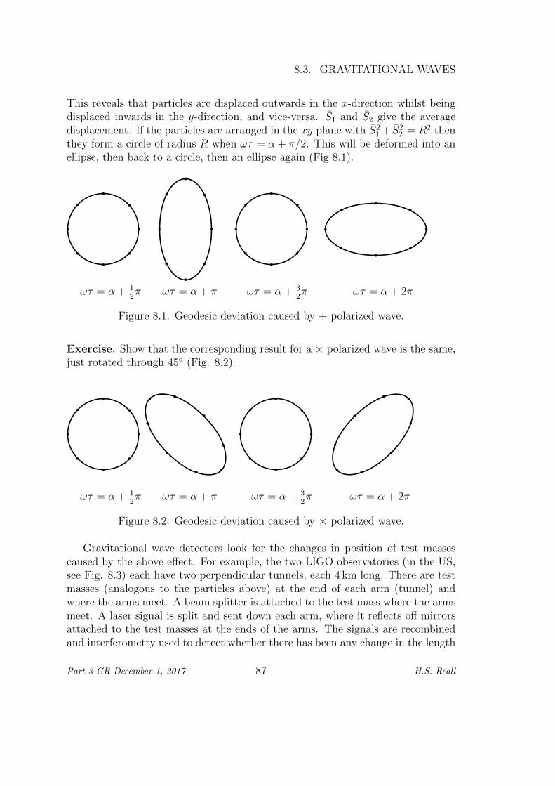
8.3. GRAVITATIONAL WAVES
This reveals that particles are displaced outwards in the x-direction whilst beingdisplaced inwards in the y-direction, and vice-versa. S1 and S2 give the averagedisplacement. If the particles are arranged in the xy plane with S2
1 + S22 = R2 then
they form a circle of radius R when ωτ = α+ π/2. This will be deformed into anellipse, then back to a circle, then an ellipse again (Fig 8.1).
ωτ = α + π ωτ = α + 32π ωτ = α + 2πωτ = α + 1
2π
Figure 8.1: Geodesic deviation caused by + polarized wave.
Exercise. Show that the corresponding result for a × polarized wave is the same,just rotated through 45 (Fig. 8.2).
ωτ = α + 12π ωτ = α + π ωτ = α + 3
2π ωτ = α + 2π
Figure 8.2: Geodesic deviation caused by × polarized wave.
Gravitational wave detectors look for the changes in position of test massescaused by the above effect. For example, the two LIGO observatories (in the US,see Fig. 8.3) each have two perpendicular tunnels, each 4 km long. There are testmasses (analogous to the particles above) at the end of each arm (tunnel) andwhere the arms meet. A beam splitter is attached to the test mass where the armsmeet. A laser signal is split and sent down each arm, where it reflects off mirrorsattached to the test masses at the ends of the arms. The signals are recombinedand interferometry used to detect whether there has been any change in the length
Part 3 GR December 1, 2017 87 H.S. Reall
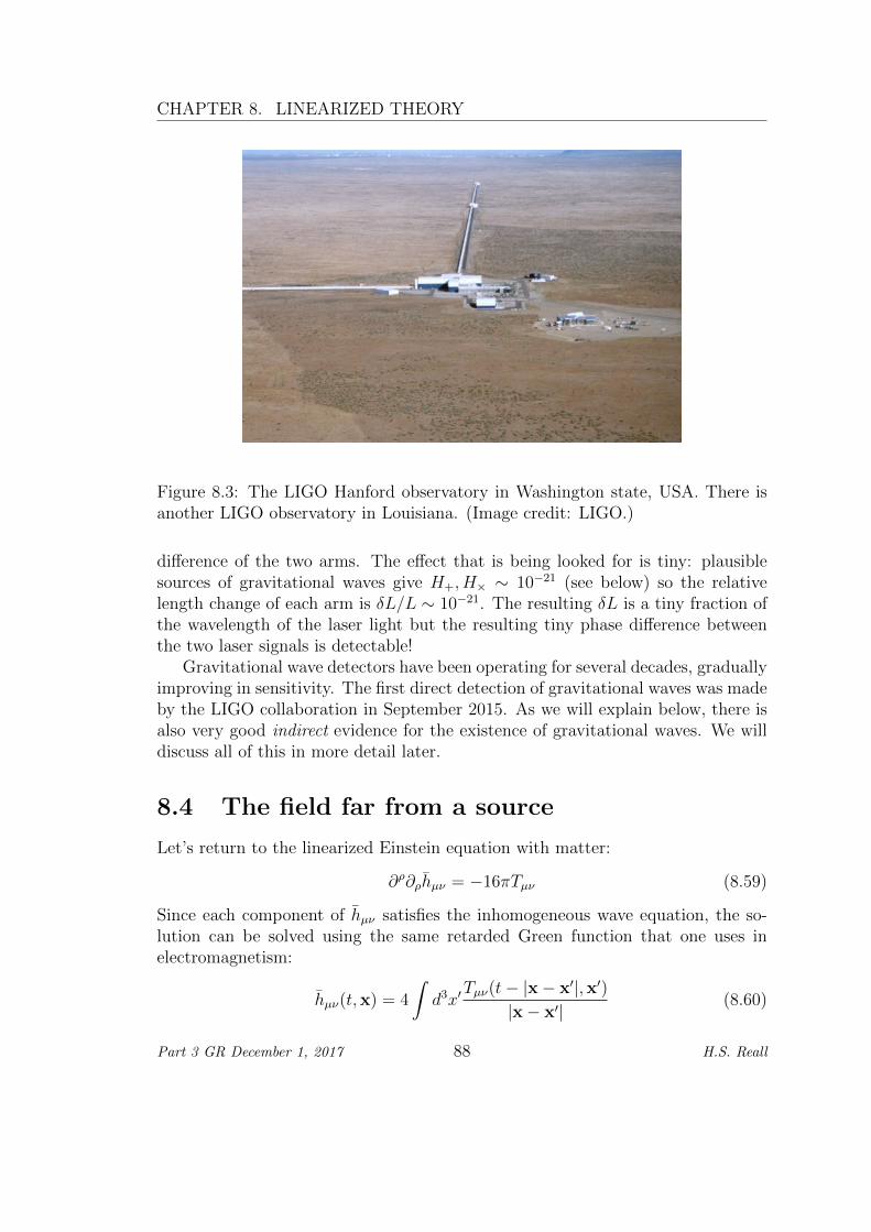
CHAPTER 8. LINEARIZED THEORY
Figure 8.3: The LIGO Hanford observatory in Washington state, USA. There isanother LIGO observatory in Louisiana. (Image credit: LIGO.)
difference of the two arms. The effect that is being looked for is tiny: plausiblesources of gravitational waves give H+, H× ∼ 10−21 (see below) so the relativelength change of each arm is δL/L ∼ 10−21. The resulting δL is a tiny fraction ofthe wavelength of the laser light but the resulting tiny phase difference betweenthe two laser signals is detectable!
Gravitational wave detectors have been operating for several decades, graduallyimproving in sensitivity. The first direct detection of gravitational waves was madeby the LIGO collaboration in September 2015. As we will explain below, there isalso very good indirect evidence for the existence of gravitational waves. We willdiscuss all of this in more detail later.
8.4 The field far from a source
Let’s return to the linearized Einstein equation with matter:
∂ρ∂ρhµν = −16πTµν (8.59)
Since each component of hµν satisfies the inhomogeneous wave equation, the so-lution can be solved using the same retarded Green function that one uses inelectromagnetism:
hµν(t,x) = 4
∫d3x′
Tµν(t− |x− x′|,x′)|x− x′|
(8.60)
Part 3 GR December 1, 2017 88 H.S. Reall
8.4. THE FIELD FAR FROM A SOURCE
where |x− x′| is calculated using the Euclidean metric.Assume that the matter is confined to a compact region near the origin of size
d (e.g. let d be the radius of the smallest sphere that encloses the matter). Then,far from the source we have r ≡ |x| |x′| ∼ d so we can expand
|x− x′|2 = r2 − 2x · x′ + x′2
= r2(1− (2/r)x · x′ +O(d2/r2)
)(8.61)
(where x = x/r) hence
|x− x′| = r − x · x′ +O(d2/r) (8.62)
Tµν(t− |x− x′|,x′) = Tµν(t′,x′) + x · x′(∂0Tµν)(t
′,x′) + . . . (8.63)
wheret′ = t− r (8.64)
Now let τ denote the time scale on which Tµν is varying so ∂0Tµν ∼ Tµν/τ . Forexample, if the source is a binary star system, then τ is the orbital period. Thesecond term in (8.63) is of order (d/τ)Tµν . Note that d is the time it takes lightto cross the region containing the matter. Hence d/τ 1 will be satisfied if thematter is moving non-relativistically. We assume this henceforth. This impliesthat the second term in (8.63) is negligible compared to the first and so
hij(t,x) ≈ 4
r
∫d3x′ Tij(t
′,x′) t′ = t− r (8.65)
Here we are considering just the spatial components of hµν , i.e., hij. Other com-ponents can be obtained from the gauge condition (8.16), which gives
∂0h0i = ∂jhji, ∂0h00 = ∂ih0i (8.66)
Given hij, the first equation can be integrated to determine h0i and the secondcan then be integrated to determine h00.
The integral in (8.65) can be evaluated as follows. Since the matter is compactlysupported, we can freely integrate by parts and discard surface terms (note alsothat t′ does not depend on x′). We can also use energy-momentum conservation,which to this order is just ∂νT
µν = 0. Let’s drop the primes on the coordinates inthe integral for now.∫
d3xT ij =
∫d3x
[∂k(T
ikxj)− (∂kTik)xj
]= −
∫d3x (∂kT
ik)xj drop surface term
=
∫d3x(∂0T
i0)xj conservation law
= ∂0
∫d3xT 0ixj (8.67)
Part 3 GR December 1, 2017 89 H.S. Reall
CHAPTER 8. LINEARIZED THEORY
We can now symmetrize this equation on ij to get∫d3xT ij = ∂0
∫d3xT 0(ixj)
= ∂0
∫d3x
[1
2∂k(T 0kxixj
)− 1
2(∂kT
0k)xixj]
= −1
2∂0
∫d3x (∂kT
0k)xixj integration by parts
=1
2∂0
∫d3x (∂0T
00)xixj conservation law
=1
2∂0∂0
∫d3xT 00xixj
=1
2Iij(t) (8.68)
where
Iij(t) =
∫d3xT00(t,x)xixj (8.69)
(Note that T00 = T 00 and Tij = T ij to leading order.) Hence we have
hij(t,x) ≈ 2
rIij(t− r) (8.70)
This result is valid when r d and τ d.Iij is the second moment of the energy density. It is a tensor in the Cartesian
sense, i.e., it transforms in the usual way under rotations of the coordinates xi.(The zeroth moment is the total energy in matter
∫d3xT00, the first moment is
the energy dipole∫d3xT00x
i.)The result (8.70) describes a disturbance propagating outwards from the source
at the speed of light. If the source exhibits oscillatory motion (e.g. a binary starsystem) then hij will describe waves with the same period τ as the motion of thesource.
The first equation in (8.66) gives
∂0h0i ≈ ∂j
(2
rIij(t− r)
)(8.71)
so integrating with respect to time gives (using ∂ir = xi/r ≡ xi)
h0i ≈ ∂j
(2
rIij(t− r)
)= −2xj
r2Iij(t− r)−
2xjrIij(t− r) + ki(x)
≈ −2xjrIij(t− r) + ki(x) (8.72)
Part 3 GR December 1, 2017 90 H.S. Reall
8.4. THE FIELD FAR FROM A SOURCE
where ki(x) is an arbitrary function. In the final line we have assumed that weare in the radiation zone r τ . This allows us to neglect the term proportionalto I because it is smaller than the term we have retained by a factor τ/r. Inthe radiation zone, space and time derivatives are of the same order of magnitude.(Note that, even for a non-relativistic source, the Newtonian approximation breaksdown in the radiation zone because (8.20) is violated.)
Similarly integrating the second equation in (8.66) gives
h00 ≈ ∂i
(−2xj
rIij(t− r)
)+ t∂iki + f(x) ≈ 2xixj
rIij(t− r) + t∂iki + f(x) (8.73)
for some arbitrary function f(x). To determine the functions f and ki we returnto (8.60), which to leading order gives
h00 ≈4E
r(8.74)
where E is the total energy of the matter
E =
∫d3x′T00(t′,x′) (8.75)
Note that energy-momentum conservation gives
∂0E =
∫d3x′(∂0T00)(t′,x′) =
∫d3x′(∂iTi0)(t′,x′) = 0 (8.76)
and hence E is a constant. We can now read off the time-independent term in h00:f(x) = 4E/r. Why have we not rediscovered the Iij term in (8.73) from (8.60)?This term is smaller than f by a factor of d2/τ 2 (convince yourself why!) so we’dhave to go to higher order in the expansion of (8.60) to find this term (and alsothe term linear in t, which appears at higher order).
Similarly, (8.60) gives
h0i ≈ −4Pir
(8.77)
where Pi is the total 3-momentum
Pi = −∫d3x′T0i(t
′,x′) (8.78)
This is also constant by energy-momentum conservation. Comparing with theabove we can read off ki(x) = −4Pi/r so we’ve now determined all components ofhµν .
Remark. We will show below that gravitational waves carry away energy (theyalso carry away momentum). So why is the total energy of matter constant? In
Part 3 GR December 1, 2017 91 H.S. Reall
CHAPTER 8. LINEARIZED THEORY
fact, the total energy of matter is not constant but one has to go beyond linearizedtheory to see this: one would have to correct the equation for energy-momentumconservation to take account of the perturbation to the connection. But then wewould have to correct the LHS of the linearized Einstein equation, including secondorder terms for consistency with the new conservation law of the RHS. So to seethis effect requires going beyond linearized theory.
A final simplification is possible: we are free to choose our almost inertialcoordinates to correspond to the ”centre of momentum frame”, i.e., Pi = 0. Ifwe do this then E is just the total mass of the matter, which we shall denote M .Putting everything together we have
h00(t,x) ≈ 4M
r+
2xixjr
Iij(t− r), h0i(t,x) ≈ −2xjrIij(t− r) (8.79)
To recap, we have assumed r τ d and work in the centre of momentum frame.In h00 we have retained the second term, even though it is subleading relative tothe first, because this is the leading order time-dependent term.
8.5 The energy in gravitational waves
We see that the gravitational waves arise when Iij varies in time. Gravitationalwaves carry energy away from the souce. Calculating this is subtle: as discussedpreviously, there is no local energy density for the gravitational field. To explainthe calculation we must go to second order in perturbation theory. At secondorder, our metric ηµν + hµν will not satisfy the Einstein equation so we have toadd a second order correction, writing
gµν = ηµν + hµν + h(2)µν (8.80)
The idea is that if the components of hµν are O(ε) then the components of h(2)µν are
O(ε2).Now we calculate the Einstein tensor to second order. The first order term is
what we calculated before (equation (8.8)). We shall call this G(1)µν [h]. The second
order terms are either linear in h(2) or quadratic in h. The terms linear in h(2) canbe calculated by setting h to zero. This is exactly the same calculation we didbefore but with h replaced by h(2). Hence the result will be (8.8) with h → h(2),
which we denote G(1)µν [h(2)]. Therefore to second order we have
Gµν [g] = G(1)µν [h] +G(1)
µν [h(2)] +G(2)µν [h] (8.81)
where G(2)µν [h] is the part of Gµν that is quadratic in h. This is:
G(2)µν [h] = R(2)
µν [h]− 1
2R(1)[h]hµν −
1
2R(2)[h]ηµν (8.82)
Part 3 GR December 1, 2017 92 H.S. Reall
8.5. THE ENERGY IN GRAVITATIONAL WAVES
where R(2)µν [h] is the term in the Ricci tensor that is quadratic in h. R(1) and R(2)
are the terms in the Ricci scalar which are linear and quadratic in h respectively.The latter can be written
R(2)[h] = ηµνR(2)µν [h]− hµνR(1)
µν [h] (8.83)
Exercise (examples sheet 3). Show that
R(2)µν [h] =
1
2hρσ∂µ∂νhρσ − hρσ∂ρ∂(µhν)σ +
1
4∂µhρσ∂νh
ρσ + ∂σhρν∂[σhρ]µ
+1
2∂σ (hσρ∂ρhµν)−
1
4∂ρh∂ρhµν −
(∂σh
ρσ − 1
2∂ρh
)∂(µhν)ρ (8.84)
For simplicity, assume that no matter is present. At first order, the linearizedEinstein equation is G
(1)µν [h] = 0 as before. At second order we have
G(1)µν [h(2)] = 8πtµν [h] (8.85)
where
tµν [h] ≡ − 1
8πG(2)µν [h] (8.86)
Equation (8.85) is the equation of motion for h(2). If h satisfies the linear Einstein
equation then we have R(1)µν [h] = 0 so the above results give
tµν [h] = − 1
8π
(R(2)µν [h]− 1
2ηρσR(2)
ρσ [h]ηµν
)(8.87)
Consider now the contracted Bianchi identity gµρ∇ρGµν = 0. Expanding this, atfirst order we get
∂µG(1)µν [h] = 0 (8.88)
for arbitrary first order perturbation h (i.e. not assuming that h satisfies anyequation of motion). At second order we get
∂µ(G(1)µν [h(2)] +G(2)
µν [h])
+ hG(1)[h] = 0 (8.89)
where the final term denotes schematically the terms that arise from the first orderchange in the inverse metric and the Christoffel symbols in gµρ∇ρ. Now, since
(8.88) holds for arbitrary h, it holds if we replace h with h(2) so ∂µG(1)µν [h(2)] = 0.
If we now assume that h satisfies its equation of motion G(1)[h] = 0 then the finalterm in (8.89) vanishes and this equation reduces to
∂µtµν = 0. (8.90)
Part 3 GR December 1, 2017 93 H.S. Reall
CHAPTER 8. LINEARIZED THEORY
Hence tµν is a symmetric tensor (in the sense of special relativity) that is (i)quadratic in the linear perturbation h, (ii) conserved if h satisfies its equation ofmotion, and (iii) appears on the RHS of the second order Einstein equation (8.85).This is a natural candidate for the energy momentum tensor of the linearizedgravitational field.
Unfortunately, tµν suffers from a major problem: it is not invariant under agauge transformation (8.14). This is how the impossibility of localizing gravita-tional energy arises in linearized theory.
Nevertheless, it can be shown that the integral of t00 over a surface of constanttime t = x0 is gauge invariant provided one considers hµν that decays at infinity,and restricts to gauge transformations which preserve this property. This integralprovides a satisfactory notion of the total energy in the linearized gravitationalfield. Hence gravitational energy does exist, but it cannot be localized.
One can use the second order Einstein equation (8.85) to convert the integraldefining the energy, which is quadratic in hµν , into a surface integral at infinity
which is linear in h(2)µν . In fact the latter can be made fully nonlinear: these surface
integrals make sense in any spacetime which is ”asymptotically flat”, irrespectiveof whether or not the linearized approximation holds in the interior. This notionof energy is referred to as the ADM energy. This is constant in time but there isa related quantity called the Bondi energy, a non-increasing function of time. Therate of change of this can be interpreted as the rate of energy loss in gravitationalwaves.
We shall follow a less rigorous, but more intuitive, approach in which we converttµν into a gauge-invariant quantity by averaging. For any point p, consider someregion R of R4 of typical coordinate size a (in all directions) centred on p. Definethe average of a tensor Xµν at p by
〈Xµν〉 =
∫R
Xµν(x)W (x)d4x (8.91)
where the averaging function W (x) is positive, satisfies∫RWd4x = 1, and tends
smoothly to zero on ∂R. Note that it makes sense to integrate Xµν because we aretreating it as a tensor in Minkowski spacetime, so we can add tensors at differentpoints.
We are interested in averaging in the region far from the source, in which wehave gravitational radiation with some typical wavelength λ (in the notation usedabove λ ∼ τ). Assume that the components of Xµν have typical size x. Since thewavelength of the radiation is λ, ∂µXνρ will have components of typical size x/λ.But the average is
〈∂µXνρ〉 = −∫R
Xνρ(x)∂µW (x)d4x (8.92)
Part 3 GR December 1, 2017 94 H.S. Reall
8.5. THE ENERGY IN GRAVITATIONAL WAVES
where we have integrated by parts and used W = 0 on ∂R. Now ∂µW has com-ponents of order W/a so the RHS above has components of order x/a. Henceif we choose a λ then averaging has the effect of reducing ∂µXνρ by a factorof λ/a 1. So if we choose a λ then we can neglect total derivatives insideaverages. This implies that we are free to integrate by parts inside averages:
〈A∂B〉 = 〈∂(AB)〉 − 〈(∂A)B〉 ≈ −〈(∂A)B〉 (8.93)
because 〈∂(AB)〉 is a factor λ/a smaller than 〈B∂A〉. Henceforth we assume a λso we can exploit these properties.
Exercises (examples sheet 3).
1. Use the linearized Einstein equation to show that, in vacuum,
〈ηµνR(2)µν [h]〉 = 0 (8.94)
Hence the second term in tµν [h] averages to zero.
2. Show that
〈tµν〉 =1
32π〈∂µhρσ∂ν hρσ −
1
2∂µh∂ν h− 2∂σh
ρσ∂(µhν)ρ〉 (8.95)
3. Show that 〈tµν〉 is gauge invariant.
Hence we can obtain a gauge invariant energy momentum tensor as long aswe average over a region much larger than the wavelength of the the gravitationalradiation we are studying. This might be a rather large region: the LIGO detectorlooks for waves with frequency around 100Hz, corresponding to a wavelength λ ∼3000km.
Exercise. Calculate 〈tµν〉 for the plane gravitational wave solution discussedabove. Show that
〈tµν〉 =1
32π
(|H+|2 + |H×|2
)kµkν =
ω2
32π
(|H+|2 + |H×|2
)1 0 0 −10 0 0 00 0 0 0−1 0 0 1
(8.96)
As one would expect, there is a constant flux of energy and momentum travellingat the speed of light in the z-direction.
Part 3 GR December 1, 2017 95 H.S. Reall
CHAPTER 8. LINEARIZED THEORY
8.6 The quadrupole formula
Now we are ready to calculate the energy loss from a compact source due togravitational radiation. The averaged energy flux 3-vector is −〈t0i〉. Consider alarge sphere r = constant far outside the source. The unit normal to the sphere(in a surface of constant t) is xi. Hence the average total energy flux across thissphere, i.e., the average power radiated across the sphere is
〈P 〉 = −∫r2dΩ〈t0i〉xi (8.97)
where dΩ is the usual volume element on a unit S2.Calculating this is just a matter of substituting the results of section 8.4 into
(8.95). Since these results apply in harmonic gauge, we have
〈t0i〉 =1
32π〈∂0hρσ∂ih
ρσ − 1
2∂0h∂ih〉
=1
32π〈∂0hjk∂ihjk − 2∂0h0j∂ih0j + ∂0h00∂ih00 −
1
2∂0h∂ih〉 (8.98)
Since hjk(t,x) = (2/r)Ijk(t− r) we have
∂0hjk =2
r
...
I jk (t− r) (8.99)
and
∂ihjk =
(−2
r
...
I jk (t− r)− 2
r2Ijk(t− r)
)xi (8.100)
The second term is smaller than the first by a factor τ/r 1 and so negligible forlarge enough r. Hence
− 1
32π
∫r2dΩ〈∂0hjk∂ihjk〉xi =
1
2〈...
I ij...
I ij〉t−r (8.101)
On the RHS, the average is a time average, taken over an interval a λ ∼ τcentered on the retarded time t− r.
Next we have h0j = (−2xk/r)Ijk(t− r) hence
∂0h0j = −2xkr
...
I jk (t− r) ∂ih0j ≈2xkr
...
I jk (t− r)xi (8.102)
where in the second expressions we have used τ/r 1 to neglect the terms arisingfrom differentiation of xk/r. Hence
− 1
32π
∫r2dΩ〈−2∂0h0j∂ih0j〉xi = − 1
4π〈...
I jk...
I jl〉t−r∫dΩxkxl (8.103)
Part 3 GR December 1, 2017 96 H.S. Reall
8.6. THE QUADRUPOLE FORMULA
Now recall the following from Cartesian tensors:∫dΩxkxl is isotropic (rotationally
invariant) and hence must equal λδkl for some constant λ. Taking the trace fixesλ = 4π/3. Hence the RHS above is
−1
3〈...
I ij...
I ij〉t−r (8.104)
Next we use h00 = 4M/r + (2xjxk/r)Ijk(t− r) to give
∂0h00 =2xjxkr
...
I jk (t− r) (8.105)
and
∂ih00 ≈(−4M
r2− 2xjxk
r
...
I jk (t− r))xi ≈ −
2xjxkr
...
I jk (t− r)xi (8.106)
where we’ve neglected terms arising from differentiation of xjxk/r in the firstequality because in the radiation zone (τ/r 1) they’re negligible compared tothe second term we’ve retained. In the second equality we’ve neglected the firstterm in brackets because this leads to a term in the integral proportional to 〈
...
I jk〉,which is the average of a derivative and therefore negligible. Hence we have
− 1
32π
∫r2dΩ〈∂0h00∂ih00〉xi =
1
8π〈...
I ij...
I kl〉t−rXijkl (8.107)
where
Xijkl =
∫dΩxixjxkxl (8.108)
is another isotropic integral which we’ll evaluate below.Next we use h = hjj − h00 and the above results to obtain
∂0h =2
r
...
I jj (t− r)− 2xjxkr
...
I jk (t− r) (8.109)
∂ih =
(−2
r
...
I jj (t− r) +2xjxkr
...
I jk (t− r))xi (8.110)
and hence (using the result above for∫dΩxixj)
− 1
32π
∫r2dΩ〈−1
2∂0h∂ih〉xi = 〈−1
4
...
I jj...
I kk +1
6
...
I jj...
I kk −1
16π
...
I ij...
I kl Xijkl〉(8.111)
Putting everything together we have
〈P 〉t = 〈16
...
I ij...
I ij −1
12
...
I ii...
I jj +1
16π
...
I ij...
I kl Xijkl〉t−r (8.112)
Part 3 GR December 1, 2017 97 H.S. Reall
CHAPTER 8. LINEARIZED THEORY
To evaluate Xijkl, we use the fact that any isotropic Cartesian tensor is a productof δ factors and ε factors. In the present case, Xijkl has rank 4 so we can onlyuse δ terms so we must have Xijkl = αδijδkl + βδikδjl + γδilδjk for some α, β, γ.The symmetry of Xijkl implies that α = β = γ. Taking the trace on ij and on klindices then fixes α = 4π/15. The final term above is therefore
1
60〈...
I ii...
I jj +2...
I ij...
I ij〉 (8.113)
and hence
〈P 〉t =1
5〈...
I ij...
I ij −1
3
...
I ii...
I jj〉t−r (8.114)
Finally we define the energy quadrupole tensor, which is the traceless part of Iij
Qij = Iij −1
3Ikkδij (8.115)
We then have
〈P 〉t =1
5〈...
Qij
...
Qij〉t−r (8.116)
This is the quadrupole formula for energy loss via gravitational wave emission. Itis valid in the radiation zone far from a non-relativistic source, i.e., for r τ d.
We conclude that a body whose quadrupole tensor is varying in time will emitgravitational radiation. A spherically symmetric body has Qij = 0 and so will notradiate, in agreement with Birkhoff’s theorem, which asserts that the unique spher-ically symmetric solution of the vacuum Einstein equation is the Schwarzschildsolution. Hence the spacetime outside a spherically symmetric body is time inde-pendent because it is described by the Schwarzschild solution.
8.7 Comparison with electromagnetic radiation
In electromagnetic theory, given a charge distribution ρ we can define the totalcharge
Q =
∫d3xρ (8.117)
and the electric dipole moment
D =
∫d3xρx (8.118)
Similarly for a matter distribution with energy density T00 we have defined thetotal energy
E =
∫d3xT00 (8.119)
Part 3 GR December 1, 2017 98 H.S. Reall
8.7. COMPARISON WITH ELECTROMAGNETIC RADIATION
and we can define the centre of mass
X(t) = E−1
∫d3xT00(t,x)x (8.120)
Electromagnetic radiation is produced by the motion of charge. Of course charge isconserved so Q does not vary with time, just like E does not vary with time. Hencethere is no monopole radiation in either electromagnetism or gravity. However,D can change with time, and changing D leads to emission of electromagneticradiation with power
〈P 〉t =1
12πε0〈|D|2〉t−r (8.121)
Since the analogue of D is X, one might expect gravitational dipole radiation whenX varies. However, we have
EX = P = 0 (8.122)
where P is the total momentum of the mass distribution, which is conserved. Hencethere is no gravitational analogue of electric dipole radiation: it is forbidden bylinear momentum conservation.
In electromagnetic theory, a varying magnetic dipole moment also producesradiation, although this is usually much weaker than electric dipole radiation.The magnetic dipole is
µ =
∫d3x x× j (8.123)
where j is the electric current. The analogue of a magnetic dipole moment for amass distribution is
J =
∫d3x x× (ρu) (8.124)
where u is the local velocity of matter (i.e. T0i ≈ −ρui as in section 8.2). But thisis simply the total angular momentum of the matter, which is again conserved. Sothere is no gravitational analogue of magnetic dipole radiation: it is forbidden byconservation of angular momentum.
These arguments ”explain” why there is no monopole or dipole gravitationalradiation. Gravitational quadrupole radiation is analogous to electric quadrupoleradiation in electromagnetic theory, which is the leading order effect when theelectric and magnetic dipoles do not vary.
It is easy to detect electromagnetic radiation but gravitational radiation is veryhard to detect. This is because gravitational waves interact only very weakly withmatter (or with each other). This is equivalent to the familiar statement thatgravity is very weak force - the weakest known force in Nature, and much weakerthan the electromagnetic force.
Part 3 GR December 1, 2017 99 H.S. Reall
CHAPTER 8. LINEARIZED THEORY
One way to see this is to consider the energy flux F of a plane gravitationalwave. For example, take a wave with h ∼ 10−21 and ω ∼ 100Hz, the kind ofsignal the LIGO detectors search for. From the 03 component of (8.96) we have,reinstating factors of G and c to give a quantity with the correct dimensions
F ∼ ω2c
32πGh2 ∼ 0.01Wm−2 (8.125)
where we are just working to an order of magnitude. This is the same as theenergy flux around 30m from a 100W light bulb. Of course an electromagneticflux of this magnitude is easily detectable - your eyes are doing it now. (However,the light has much higher frequency so maybe a better comparison is with 100Hzelectromagnetic waves, i.e., low frequency radio waves, and these would also beeasy to detect at a flux of 0.01Wm−2.) But to detect the same energy flux ingravitational waves requires spending a billion dollars to construct a state of theart detector! A large energy flux produces only a very small effect on the detectorbecause gravity interacts with matter so weakly.
The weakness of gravity has some advantanges. Because gravitational wavesdo not interact much with matter, they do not suffer much distortion as they prop-agate through the Universe. Unlike electromagnetic waves, they are not absorbedor scattered by matter. So the waves received by a detector are essentially thesame as the waves emitted by the source, adjusted for cosmological expansion.
8.8 Gravitational waves from binary systems
A fairly common astrophysical system with a time-varying quadrupole is a binarysystem, consisting of a pair of stars orbiting their common centre of mass. Con-sider the case when the stars both have mass M , their separation is d and theorbital period is τ so the angular velocity is ω ∼ τ−1. Then Newton’s secondlaw gives Mω2d ∼ M2/d2 which gives ω ∼ M1/2d−3/2. The quadrupole tensorhas components of typical size Md2 so the third derivative is of size Md2/τ 3 ∼Md2ω3 ∼ (M/d)5/2. Hence we obtain the order of magnitude estimate
P ∼ (M/d)5. (8.126)
The power radiated in gravitational waves is greatest when M/d is as large aspossible. Note the large power (5) on the RHS of this equation: if M/d decreasesby an order of magnitude then P decreases by 5 orders of magnitude. To get alarge P we need the system to have M/d as small as possible, i.e., it has to be ascompact as possible.
To understand the size of P , recall that we’ve used units G = c = 1 in (8.126).Reinstating units gives
P ∼ (M/d)5LPlanck (8.127)
Part 3 GR December 1, 2017 100 H.S. Reall
8.8. GRAVITATIONAL WAVES FROM BINARY SYSTEMS
where LPlanck is the Planck luminosity
LPlanck =c5
G≈ 4× 1052 W (8.128)
This is a mind-bogglingly enormous luminosity. The electromagnetic luminosity ofthe Sun is L ≈ 4× 1026W ≈ 10−26LPlanck. There are roughly 1010 galaxies in theobservable Universe, so if a typical galaxy contains 1011 stars we can estimate theelectromagnetic luminosity of all the stars in the Universe as 1021L ≈ 10−5LPlanck.
Hence a binary with M/d>∼ 10−1 would emit more power in gravitational radiation
than all the stars in the Universe emit in electromagnetic radiation!How big can M/d be? Obviously d cannot be smaller than the size R of the
stars themselves. However, a normal star has radius R M . For example, theSun has R ≈ 7× 10⁵km and M ≈ 1.5km so M/R ∼ 2× 10⁻⁶ hence a binary madeof Sun-like stars would have M/d 10−6 as d R. To obtain a larger amountof radiation we need to consider binary systems made of much more compactbodies, i.e., bodies with M/R as large as possible. The most compact objects inNature are black holes, whose size is given by the Schwarzschild radius R = 2M(anything more compact than this would collapse to form a black hole: see theBlack Holes course). Almost as compact are neutron stars: stars made of nuclearmatter held together by gravity, like a giant atomic nucleus. So the binaries whichare expected to emit the most gravitational radiation are tightly bound NS/NS,NS/BH or BH/BH systems (NS: neutron star, BH: black hole).
The emission of gravitational radiation causes the shape of the orbit to changeover time. To a good approximation, valid when the stars are far apart and movingnon-relativistically, we can calculate this by letting the radius of the Newtonianorbit vary slowly with time. The energy of a Newtonian orbit is E ∼ −M2/dso d decreases as the system loses energy via gravitational radiation. Hence theorbital period τ ∼ d3/2M−1/2 also decreases. To calculate how d varies with time,we equate dE/dt with −P . (See Examples sheet 4.) This approximation can beimproved by including higher order, post-Newtonian, effects.
This prediction of GR has been confirmed observationally. In 1974, Hulseand Taylor detected a binary pulsar. This is a NS/NS binary in which one ofthe stars is a pulsar, i.e., it emits a beam of radio waves in a certain direction.This star is rotating very rapidly and the beam (which is not aligned with therotation axis) periodically points in our direction. Hence we receive pulses ofradiation from the star. The period between successive pulses (about 0.05s) isvery stable and has been measured to very high accuracy. Therefore it acts likea clock that we can observe from Earth. Using this clock we can determine theorbital period (about 7.75h) of the binary system, again with good accuracy. Theemission of gravitational waves causes the period of the orbit to decrease by about10µs per year. This small effect has been measured and the result confirms the
Part 3 GR December 1, 2017 101 H.S. Reall
CHAPTER 8. LINEARIZED THEORY
quadrupole formula to an accuracy of 0.3% (the accuracy increases the longer thesystem is observed). This is very strong indirect evidence for the existence ofgravitational waves, for which Hulse and Taylor received the Nobel Prize in 1993.(The gravitational wave luminosity of the Hulse-Taylor system is about 0.02L.)
As a compact binary system loses energy to radiation, the radius of the orbitshrinks and eventually the two bodies in the system will collide and merge to forma single black hole (it is unlikely to be a neutron star because a NS cannot have amass greater than about 2M). As the system approaches merger, the velocitiesof the two bodies become very large, a significant fraction of the speed of light.For such a system, the post-Newtonian expansion is useless and the only way ofpredicting what will happen is to solve the Einstein equation numerically on asupercomputer. As the bodies approach merger, the luminosity P still increasesin rough agreement with (8.126), with the luminosity peaking at the merger. (Nu-merical simulations indicate that the largest possible peak luminosity in a BH/BHmerger is about 0.002LPlanck.) Hence the strongest sources of gravitational wavesare expected to be compact binaries just before merger.
To discuss the direct detection of gravitational waves from a merging compactbinary, we need to estimate the amplitude of the gravitational waves from such asource. At a distance r, the above estimates give
hij ∼Md2
τ 2r∼ M2
dr(8.129)
We can use this to estimate the amplitude of waves arriving at a detector on Earth.We take r to be the distance within which we expect there to exist sufficiently manysuitable binary system that at least one will merge within a reasonable time, say1 year (we don’t want to have to wait for 100 years to detect anything!). Theprocess of gradual inspiral to final merger is very slow, taking billions of years forplausible initial conditions (see Examples sheet 4). This implies that r must be ofcosmological size: of the order of 3 × 10⁸ light years. Taking M to be about tentimes the mass of the Sun and d to be ten times the Schwarzschild radius givesh ∼ 10−21 and waves with a frequency of 100− 1000 Hz. This is the kind of signalthat the two LIGO detectors (in the US) and the Virgo detector (in Italy) aredesigned to detect.
On examples sheet 4 you will investigate how properties of the source can bededuced from properties of the gravitational waves detected. From the frequency ofthe waves one can deduce the orbital frequency ω. If, during the “inspiral” phase,one knows the frequency of the waves, and the rate of change of this frequency,then one can deduce the so-called chirp mass
Mchirp =(M1M2)3/5
(M1 +M2)1/5(8.130)
Part 3 GR December 1, 2017 102 H.S. Reall

8.8. GRAVITATIONAL WAVES FROM BINARY SYSTEMS
where M1 and M2 are the masses of the two objects. This gives a measure ofthe total mass M of the system. From the amplitude of the waves one can thenestimate the distance r of the source using (8.129) (with d ∼ (M/ω2)1/3). Thewaves emitted immediately after the merger occur as the final black hole is “settlingdown to equilibrium”. The frequency and decay time of such waves are determineduniquely by the final black hole, so this can be used to determine the final blackhole mass. Of course, in practice, parameters of the initial compact objects andfinal black hole are determined by finding the best-fit theoretical prediction to theentire signal.
The first direct detection of gravitational waves was made by the LIGO col-laboration on 14 September 2015 (Fig. 8.4). This event is now referred to asGW150914 (the numbers are the date of the event). By comparing with thedetailed predictions of General Relativity (determined using the post-Newtonianexpansion and numerical simulations), it was deduced that these waves were emit-ted in the merger of a compact binary at a distance of 1.4× 10⁹ light years. Themasses of the objects in the binary were estimated to be 36M and 29M. Sincethese are well above the upper mass limit for a neutron star, it was deduced thatthis was a BH/BH binary. The merger produced a final BH with mass 62M. Themissing mass 3M was emitted as gravitational radiation. The detected signallasted for about 0.2s. The gravitational wave luminosity at the merger was greaterthan the electromagnetic luminosity of all the stars in the visible Universe!
Figure 8.4: The signals detected by the two LIGO observatories on 14 September2015. The vertical axis is the change in length of the arms of the detectors. (Imagecredit: LIGO.)
Several further detections of gravitational waves from BH/BH binaries havebeen made by LIGO and (from August 2017) Virgo. The properties of these
Part 3 GR December 1, 2017 103 H.S. Reall
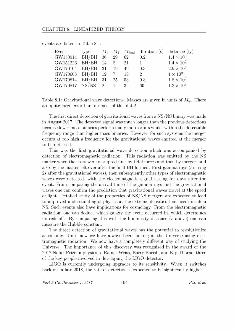
CHAPTER 8. LINEARIZED THEORY
events are listed in Table 8.1.
Event type M1 M2 Mfinal duration (s) distance (ly)GW150914 BH/BH 36 29 62 0.2 1.4× 10⁹
GW151226 BH/BH 14 8 21 1 1.4× 10⁹
GW170104 BH/BH 31 19 49 0.3 2.9× 10⁹
GW170608 BH/BH 12 7 18 2 1× 10⁹
GW170814 BH/BH 31 25 53 0.3 1.8× 10⁹
GW170817 NS/NS 2 1 3 60 1.3× 10⁸
Table 8.1: Gravitational wave detections. Masses are given in units of M. Thereare quite large error bars on most of this data!
The first direct detection of gravitational waves from a NS/NS binary was madein August 2017. The detected signal was much longer than the previous detectionsbecause lower mass binaries perform many more orbits whilst within the detectablefrequency range than higher mass binaries. However, for such systems the mergeroccurs at too high a frequency for the gravitational waves emitted at the mergerto be detected.
This was the first gravitational wave detection which was accompanied bydetection of electromagnetic radiation. This radiation was emitted by the NSmatter when the stars were disrupted first by tidal forces and then by merger, andalso by the matter left over after the final BH formed. First gamma rays (arriving2s after the gravitational waves), then subsequently other types of electromagneticwaves were detected, with the electromagnetic signal lasting for days after theevent. From comparing the arrival time of the gamma rays and the gravitationalwaves one can confirm the prediction that gravitational waves travel at the speedof light. Detailed study of the properties of NS/NS mergers are expected to leadto improved understanding of physics at the extreme densities that occur inside aNS. Such events also have implications for cosmology. From the electromagneticradiation, one can deduce which galaxy the event occurred in, which determinesits redshift. By comparing this with the luminosity distance (r above) one canmeasure the Hubble constant.
The direct detection of gravitational waves has the potential to revolutionizeastronomy. Until now we have always been looking at the Universe using elec-tromagnetic radiation. We now have a completely different way of studying theUniverse. The importance of this discovery was recognized in the award of the2017 Nobel Prize in physics to Rainer Weiss, Barry Barish, and Kip Thorne, threeof the key people involved in developing the LIGO detector.
LIGO is currently undergoing upgrades to its sensitivity. When it switchesback on in late 2018, the rate of detection is expected to be significantly higher.
Part 3 GR December 1, 2017 104 H.S. Reall
Chapter 9
Differential forms
9.1 Introduction
Definition. Let M be a differentiable manifold. A p-form on M is an antisym-metric (0, p) tensor field on M .
Remark. A 0-form is a function, a 1-form is a covector field.
Definition. The wedge product of a p-form X and a q-form Y is the (p+ q)-formX ∧ Y defined by
(X ∧ Y )a1...apb1...bq =(p+ q)!
p!q!X[a1...apYb1...bq ] (9.1)
Exercise. Show thatX ∧ Y = (−1)pqY ∧X (9.2)
(so X ∧X = 0 if p is odd); and
(X ∧ Y ) ∧ Z = X ∧ (Y ∧ Z) (9.3)
i.e. the wedge product is associative so we don’t need to include the brackets.
Remark. If we have a dual basis fµ then the set of p-forms of the form fµ1 ∧fµ2 . . . ∧ fµp give a basis for the space of all p-forms on M because we can write
X =1
p!Xµ1...µpf
µ1 ∧ fµ2 . . . ∧ fµp (9.4)
Definition. The exterior derivative of a p-form X is the (p+ 1)-form dX definedin a coordinate basis by
(dX)µ1...µp+1 = (p+ 1)∂[µ1Xµ2...µp+1] (9.5)
105
CHAPTER 9. DIFFERENTIAL FORMS
Exercise. Show that this is independent of the choice of coordinate basis.
Remark. This reduces to our previous definition of d acting on functions whenp = 0.
Lemma. If ∇ is a (torsion-free) connection then
(dX)a1...ap+1 = (p+ 1)∇[a1Xa2...ap+1] (9.6)
Proof. The components of the LHS and RHS are equal in normal coordinates at rfor any point r.
Exercises (examples sheet 4). Show that the exterior derivative enjoys the fol-lowing properties:
d(dX) = 0 (9.7)
d(X ∧ Y ) = (dX) ∧ Y + (−1)pX ∧ dY (9.8)
(where Y is a q-form) andd(φ∗X) = φ∗dX (9.9)
(where φ : N →M), i.e. the exterior derivative commutes with pull-back.
Remark. The last property implies that the exterior derivative commutes with aLie derivative:
LV (dX) = d(LVX) (9.10)
where V is a vector field.
Definition. X is closed if dX = 0 everywhere. X is exact if there exists a(p− 1)-form Y such that X = dY everywhere.
Remark. Exact implies closed. The converse is true only locally:
Poincare Lemma. If X is a closed p-form (p ≥ 1) then for any r ∈ M thereexists a neighbourhood O of r and a (p− 1)-form Y such that X = dY in O.
9.2 Connection 1-forms
Remark. Often in GR it is convenient to work with an orthonormal basis ofvector fields eaµ obeying
gabeaµebν = ηµν (9.11)
where ηµν = diag(−1, 1, . . . , 1). (In 4d, such a basis is sometimes called a tetrad.)(On a Riemannian manifold we do the same with ηµν replaced by δµν .) Since ηµνis the metric in our basis, Greek tensor indices can be lowered with ηµν and raisedwith ηµν .
Part 3 GR December 1, 2017 106 H.S. Reall
9.2. CONNECTION 1-FORMS
Exercise. Show that the dual basis fµa is given by
fµa = ηµν(eν)a ≡ eµa ⇒ eµaeaν = δµν (9.12)
Remark. Here we have defined what it means to raise the Greek index labelingthe basis vector. Henceforth any Greek index can be raised/lowered with theMinkowski metric.
Remark. We saw earlier (section 3.2) that any two orthonormal bases at arerelated by a Lorentz transformation which acts on the indices µ, ν:
e′aµ =
(A−1
)νµeaν , ηµνA
µρA
νσ = ηρσ (9.13)
There is an important difference with special relativity: the Lorentz transformationAµν need not be constant, it can depend on position. Working with orthonormalbases brings the equations of GR to a form in which Lorentz transformations area local symmetry.
Lemma.ηµνe
µaeνb = gab, eµae
bµ = δba (9.14)
Proof. Contract the LHS of the first equation with a basis vector ebρ:
ηµνeµaeνbebρ = ηµνe
µaδ
νρ = ηµρe
µa = (eρ)a = gabe
bρ (9.15)
Hence the first equation is true when contracted with any basis vector so it is truein general. This equation can be written as eµa(eµ)b = gab. Raise the b index to getthe second equation.
Definition. The connection 1-forms ωµν are (using the Levi-Civita connection)
(ωµν)a = eµb∇aebν (9.16)
Exercise. Show that
(ωµν)a = Γµνρeρa (9.17)
where Γµνρ are the connection components of equation (4.5).
Remark. The indices µ, ν on ωµν are not tensor indices: they do not transformcorrectly under Lorentz transformations. This is just the fact that the componentsof the connection are not tensor components. However, for each pair (µ, ν), we dohave a well-defined 1-form ωµν .
Lemma. (ωµν)a = −(ωνµ)a.Proof.
(ωµν)a = (eµ)b∇aebν = ∇a
((eµ)be
bν
)− ebν∇a(eµ)b = ∇aηµν − (ωνµ)a (9.18)
Part 3 GR December 1, 2017 107 H.S. Reall
CHAPTER 9. DIFFERENTIAL FORMS
and ∇aηµν = 0 because ηµν are just constant scalars.
Lemma. Regard eµa as a 1-form. Then
deµ = −ωµν ∧ eν (9.19)
Proof. From the definition of ωµν we have
∇aebν = (ωµν)a e
bµ (9.20)
hence∇a(eµ)b = (ωνµ)a e
νb = − (ωµν)a e
νb (9.21)
and so(deµ)ab = 2∇[ae
µb] = −2 (ωµν)[a e
νb] = − (ωµν ∧ eν)ab (9.22)
Remark. Evaluating (9.19) in our basis gives (cf (9.4))
deµ = −(ωµν)ρeρ ∧ eν = (ωµ[ν)ρ]e
ν ∧ eρ (9.23)
and hence(deµ)νρ = 2(ωµ[ν)ρ]. (9.24)
So if we calculated deµ then we can read off (ωµ[ν)ρ]. If we do this for all µ thenthe connection 1-forms can be read off because the antisymmetry ωµν = −ωνµimplies (ωµν)ρ = (ωµ[ν)ρ] + (ων[ρ)µ] − (ωρ[µ)ν]. Since calculating deµ is often quiteeasy, this provides a convenient method of calculating the connection 1-forms. Insimple cases, one can read off ωµν by inspection. It is always a good idea to checkthe result by substituting back into (9.19).
Example. The Schwarzschild spacetime admits the obvious tetrad
e0 = fdt, e1 = f−1dr, e2 = rdθ, e3 = r sin θdφ (9.25)
where f =√
1− 2M/r. We then have
de0 = df ∧ dt+ fd(dt) = f ′dr ∧ dt = f ′e1 ∧ e0 (9.26)
de1 = −f−2f ′dr ∧ dr = 0 (9.27)
de2 = dr ∧ dθ = (f/r)e1 ∧ e2 (9.28)
de3 = sin θdr ∧ dφ+ r cos θdθ ∧ dφ = (f/r)e1 ∧ e3 + (1/r) cot θe2 ∧ e3 (9.29)
The first of these suggests we try ω01 = f ′e0. This would give ω01 = −f ′e0
and hence ω10 = f ′e0 so ω10 = f ′e0. This would make a vanishing contribu-
tion to de1 (ω10 ∧ e0 = 0), which looks promising. The third equation suggests
Part 3 GR December 1, 2017 108 H.S. Reall
9.3. SPINORS IN CURVED SPACETIME
we try ω21 = (f/r)e2, which gives ω1
2 = −(f/r)e2 which again would make avanishing contribution to de1. The final equation suggests ω3
1 = (f/r)e3 andω3
2 = (1/r) cot θ e3 and again these will not spoil the second and third equations.So these connection 1-forms (and those related by ωµν = −ωνµ) must be the correctanswer.
Remark. From (4.8), the components of the covariant derivative of a vector fieldY a are
∇νYµ = eν(Y
µ) + ΓµρνYρ = ∂νY
µ + ωµρνYρ (9.30)
where ∂µ ≡ eαµ∂α, α refers to a coordinate basis, and ωµρν ≡ (ωµρ)ν .
Exercise. What is the corresponding result for a (1, 1) tensor field?
9.3 Spinors in curved spacetime
Remark. We’ve seen how to define tensors in curved spacetime. But what aboutspinor fields, i.e., fields of non-integer spin? If we use orthonormal bases, this isstraightforward because the structure of special relativity is manifest locally.
Remark. For now, we work at a single point p. Consider an infinitesimal Lorentztransformation at p
Aµν = δµν + αµν (9.31)
for infinitesimal α. The condition that this be a Lorentz transformation (thesecond equation in (9.13) gives the restriction
αµν = −ανµ (9.32)
So an infinitesimal Lorentz transformation at p is described by an antisymmetricmatrix. We now consider a representation of the Lorentz group at p in which theLorentz transformation A is described by a matrix D(A).
Definition. The generators of the Lorentz group in the representation D arematrices T µν = −T νµ defined by
D(A) = 1 +1
2αµνT
µν (9.33)
when A is given by (9.31).
Example. Lorentz transformations were defined by looking at transformationsof vectors. Let’s work out the generators in this defining, vector representation.Under a Lorentz transformation, the components of a vector transform as X ′µ =AµνX
ν = Xµ + αµνXν so we must have
1
2αρσ (T ρσ)µ νX
ν = αµνXν = αρση
µρδσνXν (9.34)
Part 3 GR December 1, 2017 109 H.S. Reall
CHAPTER 9. DIFFERENTIAL FORMS
and hence, remembering the antisymmetry of α, the Lorentz generators in thevector representation, which we denote Mµν , have components
(Mρσ)µ ν = ηµρδσν − ηµσδρν (9.35)
From these we deduce the Lorentz algebra (the square brackets denote a matrixcommutator)
[Mµν ,Mρσ] = . . . (9.36)
Remark. A finite Lorentz transformation can be obtained by exponentiating:
A = exp
(1
2αµνM
µν
)(9.37)
We then have
D(A) = exp
(1
2αµνT
µν
)(9.38)
In these expressions, αµν = −αµν are finite parameters describing the transforma-tion.
Definition. The Dirac gamma matrices are a set of square matrices Γµ whichobey
ΓµΓν + ΓνΓµ = 2ηµν (9.39)
Remark. In 4d spacetime, the smallest representation of the gamma matrices isgiven by the Dirac representation in which Γµ are 4× 4 matrices. It is unique upto equivalence of representations.
Lemma. The matrices
T µν = − i4
[Γµ,Γν ] (9.40)
form a representation of the Lorentz algebra (9.36). This is the Dirac representa-tion describing a particle of spin 1/2.
Remark. So far, we’ve worked at a single point p. Let’s now allow p to vary. Thefollowing definition looks more elegant if one uses the language of vector bundles.
Definition. A field in the Lorentz representation D is a smooth map which, forany point p and any orthonormal basis eµ defined in a neighbourhood of p, givesa vector ψ in the carrier space of the representation D, with the property that if(p, eµ) maps to ψ then (p, e′µ) maps to D(A)ψ where e′µ is related to eµby the Lorentz transformation A.
Example. Take D to be the vector representation. Then the carrier space is justRn so we can denote the resulting vector ψµ. Then D(A) = A and so under a
Part 3 GR December 1, 2017 110 H.S. Reall
9.4. CURVATURE 2-FORMS
change of basis we have ψ′µ = Aµνψν , which is just the usual transformation law
for the components of a vector.
Remark. Given a field transforming in some representation D, we can take apartial derivative of its components in a coordinate basis, and then convert theresult to our orthonormal basis, i.e., ∂µψ ≡ eαµ∂αψ where α refers to the coordinatebasis. However, since the matrix A can depend on position, the partial derivative ofour field will no longer transform homogeneously under a Lorentz transformation:the result will involve derivatives of A. For tensor fields, we know how to resolvethis problem: introduce the covariant derivative. So now we need to extend thedefinition of covariant derivative to a general representation D:
Definition. The covariant derivative of a field ψ transforming in a representationof the Lorentz group with generators T µν is, in an orthonormal basis,
∇µψ = ∂µψ +1
2(ωνρ)µ T
νρψ (9.41)
Remark. One can show that this does indeed transform correctly, i.e., in a rep-resentation of the Lorentz group, under Lorentz transformations. The connection1-forms are sometimes referred to as the spin connection because of their role indefining the covariant derivative for spinor fields.
Definition. The Dirac equation for a spin 1/2 field of mass m is
Γµ∇µψ −mψ = 0. (9.42)
9.4 Curvature 2-forms
Definition. Consider a spacetime with an orthonormal basis. The curvature2-forms are
Θµν =
1
2Rµ
νρσeρ ∧ eσ (9.43)
Remark. The antisymmetry of the Riemann tensor implies Θµν = −Θνµ.
Lemma. The curvature 2-forms are given in terms of the connection 1-forms by
Θµν = dωµν + ωµρ ∧ ωρν (9.44)
Proof. Optional exercise. Direct calculation of the RHS, using the relation (9.17)and equation (9.19). You’ll need to work out the generalization of (6.6) to anon-coordinate basis.
Part 3 GR December 1, 2017 111 H.S. Reall
CHAPTER 9. DIFFERENTIAL FORMS
Remark. This provides a convenient way of calculating the Riemann tensor in anorthonormal basis. One calculates the connection 1-forms using (9.19) and then thecurvature 2-forms using (9.43). The components of Θµ
ν are Rµνρσ so one can read
off the Riemann tensor components. The only derivatives one needs to calculateare exterior derivatives, which are usually fairly easy. In simple situations, this ismuch faster than calculating the Riemann tensor in a coordinate basis using (6.6).
Example. We determined the connection 1-forms in the Schwarzschild spacetimepreviously. From ω0
1 = f ′e0 we have
dω01 = f ′de0 + f ′′dr ∧ e0 = f ′
2e1 ∧ e0 + ff ′′e1 ∧ e0 (9.45)
we also haveω0
ρ ∧ ωρ1 = ω01 ∧ ω1
1 = 0 (9.46)
where the first equality arises because ω0ρ is non-zero only for ρ = 1 and the second
equality is because ω11 = ω11 = 0 (by antisymmetry). Combining these results we
haveΘ01 = −Θ0
1 =(ff ′′ + f ′
2)e0 ∧ e1 (9.47)
and hence the only non-vanishing components of the form R01ρσ are
R0101 = −R0110 =(ff ′′ + f ′
2)
=1
2
(f 2)′′
= −2M
r3(9.48)
Exercise (examples sheet 4). Determine the remaining curvature 2-forms Θ02,Θ03, Θ12, Θ13, Θ23 (all others are related to these by (9.44)). Hence determine theRiemann tensor components. Check that the Ricci tensor vanishes.
9.5 Volume form
Definition. A manifold of dimension n is orientable if it admits an orientation: asmooth, nowhere vanishing n-form εa1...an . Two orientations ε and ε′ are equivalentif ε′ = fε where f is an everywhere positive function.
Remark. Any n-form X is related to ε by X = fε for some function f . X willdefine an orientation provided f does not vanish anywhere. Hence an orientablemanifold admits precisely two inequivalent orientations, corresponding to the casesf > 0 and f < 0.
Definition. A coordinate chart xµ on an orientable manifold is right-handed withrespect to ε iff ε = f(x)dx1 ∧ dx2 ∧ . . . ∧ dxn with f(x) > 0. It is left-handed iff(x) < 0.
Part 3 GR December 1, 2017 112 H.S. Reall
9.5. VOLUME FORM
Definition. On an oriented manifold with a metric, the volume form is definedby
ε12...n =√|g| (9.49)
in any right-handed coordinate chart, where g denotes the determinant of themetric in this chart.
Exercise. 1. Show that this definition is chart-independent. 2. Show that (in aRH coordinate chart)
ε12...n = ± 1√|g|
(9.50)
where the upper (lower) sign holds for Riemannian (Lorentzian) signature.
Lemma. ∇aεb1...bn = 0 where ∇ is the Levi-Civita connection.Proof. Use normal coordinates at p: the partial derivatives of gµν vanish hence sodo those of g. Since the Christoffel symbols also vanish at p, the result follows.
Lemma.εa1...apcp+1...cnεb1...bpcp+1...cn = ±p!(n− p)!δa1[b1
. . . δapbp] (9.51)
where the upper (lower) sign holds for Riemannian (Lorentzian) signature.Proof. Exercise.
Definition. On an oriented manifold with metric, the Hodge dual of a p-form Xis the (n− p)-form ? X defined by
(? X)a1...an−p =1
p!εa1...an−pb1...bpX
b1...bp (9.52)
Lemma. For a p-form X,
?(? X) = ±(−1)p(n−p)X (9.53)
(? d ? X)a1...ap−1 = ±(−1)p(n−p)∇bXa1...ap−1b (9.54)
where the upper (lower) sign holds for Riemannian (Lorentzian) signature.Proof. Exercise (use (9.51)).
Examples.
1. In 3d Euclidean space, the usual operations of vector calculus can be writtenusing differential forms as
∇f = df div X = ? d ? X curl X = ? dX (9.55)
where f is a function and X denotes the 1-form Xa dual to a vector fieldXa. The final equation shows that the exterior derivative can be thought ofas a generalization of the curl operator.
Part 3 GR December 1, 2017 113 H.S. Reall
CHAPTER 9. DIFFERENTIAL FORMS
2. Maxwell’s equations are ∇aFab = −4πjb and ∇[aFbc] = 0 where ja is thecurrent density vector. These can be written as
d ? F = −4π ? j, dF = 0 (9.56)
The first of these implies d ? j = 0, which is equivalent to ∇aja = 0, i.e., ja
is a conserved current. The second of these implies (by the Poincare lemma)that locally there exists a 1-form A such that F = dA.
9.6 Integration on manifolds
Definition. Let M be an oriented manifold of dimension n. Let ψ : O → U be aRH coordinate chart with coordinates xµ and let X be a n-form. The integral ofX over O is ∫
OX ≡
∫Udx1 . . . dxnX12...n (9.57)
Exercise. Show that this is chart independent, i.e., if one replaces φ with anotherRH coordinate chart φ′ : O → U ′ then one gets the same result.
Remark. How do we extend our definition to all of M? The idea is just to chopM up into regions such that we can use the above definition on each region, thensum the resulting terms.
Definition. Let the RH charts φα : Oα → Uα be an atlas for M . Introduce a”partition of unity”, i.e., a set of functions hα : M → [0, 1] such that hα(p) = 0 ifp /∈ Oα, and
∑α hα(p) = 1 for all p. We then define∫
M
X ≡∑α
∫OαhαX (9.58)
Remark.
1. It can be shown that this definition is independent of the choice of atlas andpartition of unity.
2. A diffeomorphism φ : M →M is orientation preserving if φ∗(ε) is equivalentto ε for any orientation ε. It is not hard to show that the integral is invariantunder orientation preserving diffeomorphisms:∫
M
φ∗(X) =
∫M
X (9.59)
Part 3 GR December 1, 2017 114 H.S. Reall
9.7. SUBMANIFOLDS AND STOKES’ THEOREM
Definition. Let M be an oriented manifold with a metric g. Let ε be the volumeform. The volume of M is
∫Mε. If f is a function on M then∫
M
f ≡∫M
fε (9.60)
Remark. We shall sometimes use the notation∫M
f =
∫M
dnx√|g|f (9.61)
This is an abuse of notation because the RHS refers to coordinates xµ but M mightnot be covered by a single chart. It has the advantage of making it clear that theintegral depends on the metric tensor.
9.7 Submanifolds and Stokes’ theorem
Definition. Let S andM be oriented manifolds of dimensionm and n respectively,m < n. A smooth map φ : S →M is an embedding if it is one-to-one (φ(p) 6= φ(q)for p 6= q, i.e. φ[S] does not intersect itself) and for any p ∈ S there exists aneighbourhood O such that φ−1 : φ[O]→ S is smooth. If φ is an embedding thenφ[S] is an embedded submanifold of M . A hypersurface is an embedded submanifoldof dimension n− 1.
Remark. The technical details here are included for completeness, we won’t needto refer to them again. Henceforth, we will simply say ”submanifold” instead of”embedded submanifold”.
Definition. If φ[S] is a m-dimensional submanifold of M and X is a m-form onM then the integral of X over φ[S] is∫
φ[S]
X ≡∫S
φ∗(X) (9.62)
Remark. If X = dY then the fact that d and φ∗ commute gives∫φ[S]
dY =
∫S
d (φ∗(Y )) (9.63)
Definition. A manifold with boundary M is defined in the same way as a manifoldexcept that charts are maps φα : Oα → Uα where now Uα is an open subset of12Rn = (x1, . . . , xn) ∈ Rn : x1 ≤ 0. The boundary of M , denoted ∂M , is the set
Part 3 GR December 1, 2017 115 H.S. Reall
CHAPTER 9. DIFFERENTIAL FORMS
of points for which x1 = 0. This is a manifold of dimension n− 1 with coordinatecharts (x2, . . . xn). If M is oriented then the orientation of ∂M is fixed by sayingthat (x2, . . . xn) is a RH chart on ∂M when (x1, . . . , xn) is a RH chart on M .
Stokes’ theorem. Let N be an oriented n-dimensional manifold with boundaryand X a (n− 1)-form. Then ∫
N
dX =
∫∂N
X (9.64)
Remarks. We define the RHS by regarding ∂N as a hypersurface in N (the mapφ is just the inclusion map) and using (9.62). We often use this result when N issome region of a larger manifold M . Then ∂N is a hypersurface in M .
Example. Let Σ be a hypersurface in a spacetime M and consider a solution ofMaxwell’s equations (9.56)). Assume that Σ has a boundary. Then
1
4π
∫∂Σ
?F =1
4π
∫Σ
d ? F = −∫
Σ
?j ≡ Q[Σ] (9.65)
The final equality defines the total charge on Σ. Hence we have a formula relatingthe charge on Σ to the flux through the boundary of Σ. This is Gauss’ law.
Definition. X ∈ Tp(M) is tangent to φ[S] at p if X is the tangent vector at p ofa curve that lies in φ[S]. n ∈ T ∗p (M) is normal to a submanifold φ[S] if n(X) = 0for any vector X tangent to φ[S] at p.
Remark. The vector space of tangent vectors to φ[S] at p has dimension m. Thevector space of normals to φ[S] at p has dimension n−m. Any two normals to ahypersurface are proportional to each other.
Definition. A hypersurface in a Lorentzian manifold is timelike, spacelike or nullif any normal is everywhere spacelike, timelike or null respectively.
Remark. Let M is a manifold with boundary and consider a curve in ∂M withparameter t and tangent vector X. Then x1(t) = 0 so
dx1(X) = X(x1) =dx1
dt= 0. (9.66)
Hence dx1(X) vanishes for any X tangent to ∂M so dx1 is normal to ∂M . Anyother normal to ∂M will be proportional to dx1. If ∂M is timelike or spacelikethen we can construct a unit normal by dividing by the norm of dx1:
na =(dx1)a√
±gbc(dx1)b(dx1)c⇒ gabnanb = ±1 (9.67)
Part 3 GR December 1, 2017 116 H.S. Reall
9.7. SUBMANIFOLDS AND STOKES’ THEOREM
One can show that this is chart independent. Here we choose the + sign if dx1 isspacelike and the − sign if dx1 is timelike (+ if the metric is Riemannian). Notethat na ”points out of” M if ∂M is timelike (or the metric is Riemannian) but intoM if ∂M is spacelike. This is to get the correct sign in the divergence theorem:
Divergence theorem. If ∂M is timelike or spacelike then∫M
dnx√|g| ∇aX
a =
∫∂M
dn−1x√|h|naXa (9.68)
where Xa is a vector field on M , ∇ is the Levi-Civita connection, and h denotesthe determinant of the metric on ∂M induced by pulling back the metric on M .naX
a is a scalar in M so it can be pulled back to ∂M , this is the integrand on theRHS.Proof. Follow through the definitions, using (9.54), (9.53) and Stokes’ theorem.The volume form of ∂M is ε where ε2...n =
√|h| in one of the coordinate charts
occuring in the definition of a manifold with boundary. In such a chart, thecomponents hµν are the same as the components gµν with 2 ≤ µ, ν ≤ n. Usingthis, gab(dx1)a(dx
1)b = g11 = h/g.
Part 3 GR December 1, 2017 117 H.S. Reall

CHAPTER 9. DIFFERENTIAL FORMS
Part 3 GR December 1, 2017 118 H.S. Reall
Chapter 10
Lagrangian formulation
10.1 Scalar field action
You are familiar with the idea that the equation of motion of a point particle canbe obtained by extremizing an action. You may also know that the same is truefor fields in Minkowski spacetime. The same is true in GR. To see how this works,consider first a scalar field, i.e., a function Φ : M → R and define the action asthe functional
S[Φ] =
∫M
d4x√−gL (10.1)
where L is the Lagrangian:
L = −1
2gab∇aΦ∇bΦ− V (Φ) (10.2)
and V (Φ) is called the scalar potential. Now consider a variation Φ→ Φ + δΦ forsome function δΦ that vanishes on ∂M (in an asymptotically flat spacetime, ∂Mwill be ”at infinity”). The change in the action is (working to linear order in δΦ)
δS = S[Φ + δΦ]− S[Φ]
=
∫M
d4x√−g(−gab∇aΦ∇bδΦ− V ′(Φ)δΦ
)=
∫M
d4x√−g [−∇a (δΦ∇aΦ) + δΦ∇a∇aΦ− V ′(Φ)δΦ]
=
∫∂M
d3x√|h| δΦna∇aΦ +
∫M
d4x√−g (∇a∇aΦ− V ′(Φ)) δΦ
=
∫M
d4x√−g (∇a∇aΦ− V ′(Φ)) δΦ (10.3)
119
CHAPTER 10. LAGRANGIAN FORMULATION
Note that we have used the divergence theorem to ”integrate by parts”. A formalway of writing the final expression is
δS =
∫M
d4xδS
δΦδΦ (10.4)
whereδS
δΦ≡√−g (∇a∇aΦ− V ′(Φ)) (10.5)
The factor of√−g here means that this quantity is not a scalar (it is an example
of a scalar density). However (1/√−g)δS/δΦ is a scalar. We’ve written things
in this strange way in order to be consistent with how we treat the gravitationalfield.
Demanding that δS vanishes for arbitrary δΦ gives us the equation of motionδS/δΦ = 0, i.e.,
∇a∇aΦ− V ′(Φ) = 0. (10.6)
The particular choice V (Φ) = 12m2Φ2 gives the Klein-Gordon equation.
10.2 The Einstein-Hilbert action
For the gravitational field, we seek an action of the form
S[g] =
∫M
d4x√−gL (10.7)
where L is a scalar constructed from the metric. An obvious choice for the La-grangian is L ∝ R. This gives the Einstein-Hilbert action
SEH [g] =1
16π
∫M
d4x√−gR =
1
16π
∫M
Rε (10.8)
where the prefactor is included for later convenience and ε is the volume form. Theidea is that we regard our manifold M as fixed (e.g. R4) and gab is determined byextremizing S[g]. In other words, we consider two metrics gab and gab + δgab anddemand that S[g+ δg]− S[g] should vanish to linear order in δgab. Note that δgabis the difference of two metrics and hence is a tensor field.
We need to work out what happens to ε and R when we vary gµν . Recall theformula for the determinant ”expanding along the µth row”:
g =∑ν
gµν∆µν (10.9)
where we are suspending the summation convention, µ is any fixed value, and ∆µν
is the cofactor matrix, whose µν element is (−1)µ+ν times the determinant of the
Part 3 GR December 1, 2017 120 H.S. Reall
10.2. THE EINSTEIN-HILBERT ACTION
matrix obtained by deleting row µ and column ν from the metric. Note that ∆µν
is independent of the µν element of the metric. Hence
∂g
∂gµν= ∆µν = ggµν (10.10)
where on the RHS we recall the formula for the inverse matrix gµν in terms of thecofactor matrix. We can use this formula to determine how g varies under a smallchange δgµν in gµν (reinstating the summation convention):
δg =∂g
∂gµνδgµν = ggµνδgµν = ggabδgab (10.11)
(we can use abstract indices in the final equality since gabδgab is a scalar) and hence
δ√−g =
1
2
√−g gabδgab (10.12)
From the definition of the volume form we have
δε =1
2εgabδgab (10.13)
Next we need to evaluate δR. To this end, consider first the change in the Christof-fel symbols. δΓµνρ is the difference between the components of two connections (i.e.the Levi-Civita connections associated to gab + δgab and gab). Since the differenceof two connections is a tensor, it follows that δΓµνρ are components of a tensorδΓabc. These components are easy to evaluate if we introduce normal coordinatesat p for the unperturbed connection: at p we have gµν,ρ = 0 and Γµνρ = 0. For theperturbed connection we therefore have, at p, (to linear order)
δΓµνρ =1
2gµσ (δgσν,ρ + δgσρ,ν − δgνρ,σ)
=1
2gµσ (δgσν;ρ + δgσρ;ν − δgνρ;σ) (10.14)
In the second equality, the semi-colon denotes a covariant derivative with respectto the Levi-Civita connection associated to gab. The two expressions are equalbecause Γ(p) = 0. The LHS and RHS are tensors so this is a basis independentresult hence we can use abstract indices:
δΓabc =1
2gad (δgdb;c + δgdc;b − δgbc;d) (10.15)
p is arbitrary so this result holds everywhere.
Part 3 GR December 1, 2017 121 H.S. Reall
CHAPTER 10. LAGRANGIAN FORMULATION
Now consider the variation of the Riemann tensor. Again it is convenient touse normal coordinates at p, so at p we have (using δ(ΓΓ) ∼ ΓδΓ = 0 at p)
δRµνρσ = ∂ρδΓ
µνσ − ∂σδΓµνρ
= ∇ρδΓµνσ −∇σδΓ
µνρ (10.16)
where ∇ is the Levi-Civita connection of gab. Once again we can immediatelyreplace the basis indices by abstract indices:
δRabcd = ∇cδΓ
abd −∇dδΓ
abc (10.17)
and p is arbitrary so the result holds everywhere. Contracting gives the variationof the Ricci tensor:
δRab = ∇cδΓcab −∇bδΓ
cac (10.18)
Finally we haveδR = δ(gabRab) = gabδRab + δgabRab (10.19)
where δgab is the variation in gab (not the result of raising indices on δgab). Usingδ(gµρg
ρν) = δ(δνµ) = 0 it is easy to show (exercise)
δgab = −gacgbdδgcd (10.20)
Putting everything together, we have
δR = −gacgbdRabδgcd + gab (∇cδΓcab −∇bδΓ
cac)
= −Rabδgab +∇c(gabδΓcab)−∇b(g
abδΓcac)
= −Rabδgab +∇aXa (10.21)
whereXa = gbcδΓabc − gabδΓcbc (10.22)
Hence the variation of the Einstein-Hilbert action is
δSEH =1
16π
∫M
δ(εR)
=1
16π
∫M
ε
(1
2Rgabδgab −Rabδgab +∇aX
a
)=
1
16π
∫M
d4x√−g(
1
2Rgabδgab −Rabδgab +∇aX
a
)(10.23)
The final term can be converted to a surface term on ∂M using the divergencetheorem. If we assume that δgab has support in a compact region that doesn’t
Part 3 GR December 1, 2017 122 H.S. Reall
10.3. ENERGY MOMENTUM TENSOR
intersect ∂M then this term will vanish (because vanishing of δgab and its derivativeon ∂M implies that Xa will vanish on ∂M). Hence we have
δSEH =1
16π
∫M
d4x√−g(−Gab
)δgab =
∫M
δSEHδgab
δgab (10.24)
where Gab is the Einstein tensor and
δSEHδgab
= − 1
16π
√−gGab (10.25)
Hence extremization of SEH reproduces the vacuum Einstein equation.
Exercise. Show that the vacuum Einstein equation with cosmological constant isobtained by extremizing
SEHΛ =1
16π
∫M
d4x√−g (R− 2Λ) (10.26)
Remark. The Palatini procedure is a different way of deriving the Einstein equa-tion from the Einstein-Hilbert action. Instead of using the Levi-Civita connec-tion, we allow for an arbitrary torsion-free connection. The EH action is then afunctional of both the metric and the connection, which are to be varied inde-pendently. Varying the metric gives the Einstein equation (but written with anarbitrary connection). Varying the connection implies that the connection shouldbe the Levi-Civita connection. When matter is included, this works only if thematter action is independent of the connection (as is the case for a scalar field orMaxwell field) or if the Levi-Civita connection is used in the matter action.
10.3 Energy momentum tensor
Next we consider the action for matter. We assume that this is given in terms ofthe integral of a scalar Lagrangian:
Smatter =
∫d4x√−gLmatter (10.27)
here Lmatter is a function of the matter fields (assumed to be tensor fields), theirderivatives, the metric and its derivatives. An example is given by the scalar fieldLagrangian discussed above. We define the energy momentum tensor by
T ab =2√−g
δSmatter
δgab(10.28)
Part 3 GR December 1, 2017 123 H.S. Reall
CHAPTER 10. LAGRANGIAN FORMULATION
in other words, under a variation in gab we have (after integrating by parts usingthe divergence theorem to eliminate derivatives of δgab if present)
δSmatter =1
2
∫M
d4x√−gT abδgab (10.29)
This definition clearly makes T ab symmetric.
Example. Consider the scalar field action we discussed previously.
S =
∫M
εL (10.30)
with L given by (10.2). Using the results for δε and δgab derived above we have,under a variation of gab:
δS =
∫M
d4x√−g[
1
2∇aΦ∇bΦ +
1
2
(−1
2gcd∇cΦ∇dΦ− V (Φ)
)gab]δgab (10.31)
Hence
T ab = ∇aΦ∇bΦ +
(−1
2gcd∇cΦ∇dΦ− V (Φ)
)gab (10.32)
If we define the total action to be SEH + Smatter then under a variation of gab wehave
δ
δgab(SEH + Smatter) =
√−g(− 1
16πGab +
1
2T ab)
(10.33)
and hence demanding that SEH + Smatter be extremized under variation of themetric gives the Einstein equation
Gab = 8πTab (10.34)
How do we know that our definition of Tab gives a conserved tensor? It follows fromthe fact that Smatter is diffeomorphism invariant. In more detail, diffeomorphismsare a gauge symmetry so the total action S = SEH + Smatter should be diffeomor-phism invariant in the sense that S[g,Φ] = S[φ∗(g), φ∗(Φ)] where Φ denotes thematter fields and φ is a diffeomorphism. The Einstein-Hilbert action alone is dif-feomorphism invariant. Hence Smatter also must be diffeomorphism invariant. Theeasiest way of ensuring this is to take it to be the integral of a scalar Lagrangianas we assumed above.
Now consider the effect of an infinitesimal diffeomorphism. As we saw whendiscussing linearized theory (eq (8.13)), an infinitesimal diffeomorphism shifts gabby
δgab = Lξgab = ∇aξb +∇bξa (10.35)
Part 3 GR December 1, 2017 124 H.S. Reall
10.3. ENERGY MOMENTUM TENSOR
Matter fields also transform according to the Lie derivative (eq (8.12)), e.g. for ascalar field:
δΦ = LξΦ = ξa∇aΦ (10.36)
Let’s consider this scalar field case in detail. Assume that the matter Lagrangianis an arbitrary scalar constructed from Φ, the metric, and arbitrarily many of theirderivatives (e.g. there could be a term of the form ∇a∇bΦ∇a∇bΦ or RΦ2). Underan infinitesimal diffeomorphism, (after integration by parts to remove derivativesfrom δΦ and δgab)
δSmatter =
∫M
d4x
(δSmatter
δΦδΦ +
δSmatter
δgabδgab
)=
∫M
d4x
(δSmatter
δΦξb∇bΦ +
1
2
√−gT abδgab
)(10.37)
The second term can be written∫M
d4x√−gT ab∇aξb =
∫M
d4x√−g[∇a
(T abξb
)−(∇aT
ab)ξb]
= −∫M
d4x√−g(∇aT
ab)ξb (10.38)
where we assume that ξb vanishes on ∂M so the total derivative can be discarded.Now diffeomorphism invariance implies that δSmatter must vanish for arbitrary ξb.Hence we must have
δSmatter
δΦ∇bΦ−
√−g∇aT
ab = 0. (10.39)
Hence we see that if the scalar field equation of motion (δSmatter/δΦ = 0) is satisfiedthen
∇aTab = 0. (10.40)
This is a special case of a very general result. Diffeomorphism invariance plusthe equations of motion for the matter fields implies energy-momentum tensorconservation. It applies for a matter Lagrangian constructed from tensor fields ofany type (the matter fields), the metric, and arbitrarily many derivatives of thematter fields and metric.
An identical argument applied to the Einstein-Hilbert action leads to the con-tracted Bianchi identity (exercise):
∇aGab = 0. (10.41)
Hence the contracted Bianchi identity is a consequence of diffeomorphism invari-ance of the Einstein-Hilbert action.
Part 3 GR December 1, 2017 125 H.S. Reall


