60
| Date post: | 16-Dec-2015 |
| Category: |
Documents |
| Upload: | christopher-foote |
| View: | 230 times |
| Download: | 0 times |

PART 5ECONOMIC FLUCTUATIONS
AS-AD and the Business Cycle
CHAPTER 14
When you have completed your study of this chapter, you will be able to
C H A P T E R C H E C K L I S T
Provide a technical definition of recession and describe the history of the U.S. business cycle.
1
Define and explain the influences on aggregate supply.2
Define and explain the influences on aggregate demand.3
Explain how fluctuations in aggregate demand and aggregate supply create the business cycle.
4
14.1 BUSINESS-CYCLE DEFINITIONS AND FACTS
The business cycle is a periodic but irregular up-and-down movement in production and jobs.
A business cycle has two phases, expansion and recession, and two turning point, a peak and a trough.
Dating Business-Cycle Turning Points
The task of identifying and dating business-cycle phases and turning points is performed by a private research organization, the National Bureau of Economic Research (NBER).
14.1 BUSINESS-CYCLE DEFINITIONS AND FACTS
To date the business-cycle turning points, the NBER needs a definition of recession.
Recession
A decrease in real GDP that lasts for at least two quarters (six months) or a period of significant decline in total output, income, employment, and trade, usually lasting from six months to a year and marked by widespread contractions in many sectors of the economy.
14.1 BUSINESS-CYCLE DEFINITIONS AND FACTS
U.S. Business-Cycle History
The NBER has identified 33 complete cycles starting from a trough in December 1854.
Over all 33 complete cycles:• The average length of an expansion is 35 months
and the average length of a recession is 18 months.
• The average time from trough to trough is 53 months.
14.1 BUSINESS-CYCLE DEFINITIONS AND FACTS
So over the 152 years since 1854, the U.S. economy has been in:
• Recession for about one third of the time• Expansion for about two thirds of the time.
The 152-year averages hide significant changes that have occurred in the length of a cycle and the relative length of the recession and expansion phases.
14.1 BUSINESS-CYCLE DEFINITIONS AND FACTS
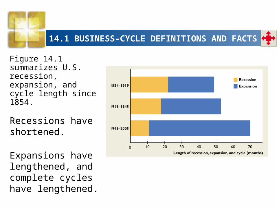
Figure 14.1 summarizes U.S. recession, expansion, and cycle length since 1854.
Recessions have shortened.
Expansions have lengthened, and complete cycles have lengthened.
14.1 BUSINESS-CYCLE DEFINITIONS AND FACTS
Recent Cycles
The last completed cycle began at a trough of March 1991 and ended at a trough of November 2001.
The economy expanded from March 1991 until March 2001.
This expansion, which lasted for 120 months, was the longest in U.S. history.
14.1 BUSINESS-CYCLE DEFINITIONS AND FACTS
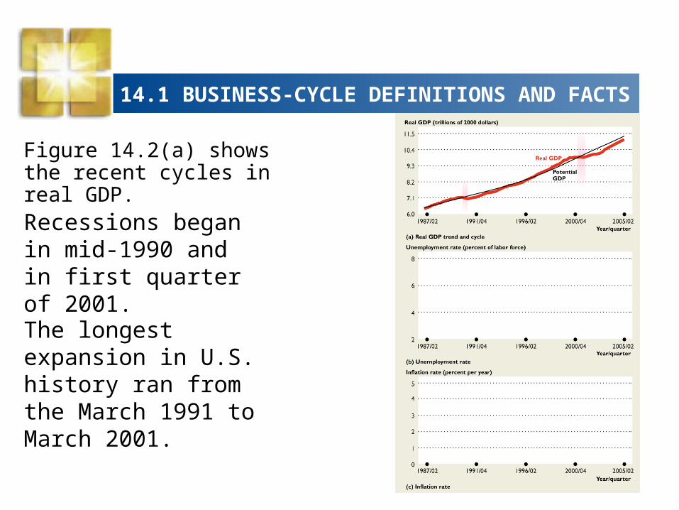
Figure 14.2(a) shows the recent cycles in real GDP.
Recessions began in mid-1990 and in first quarter of 2001.
The longest expansion in U.S. history ran from the March 1991 to March 2001.
14.1 BUSINESS-CYCLE DEFINITIONS AND FACTS
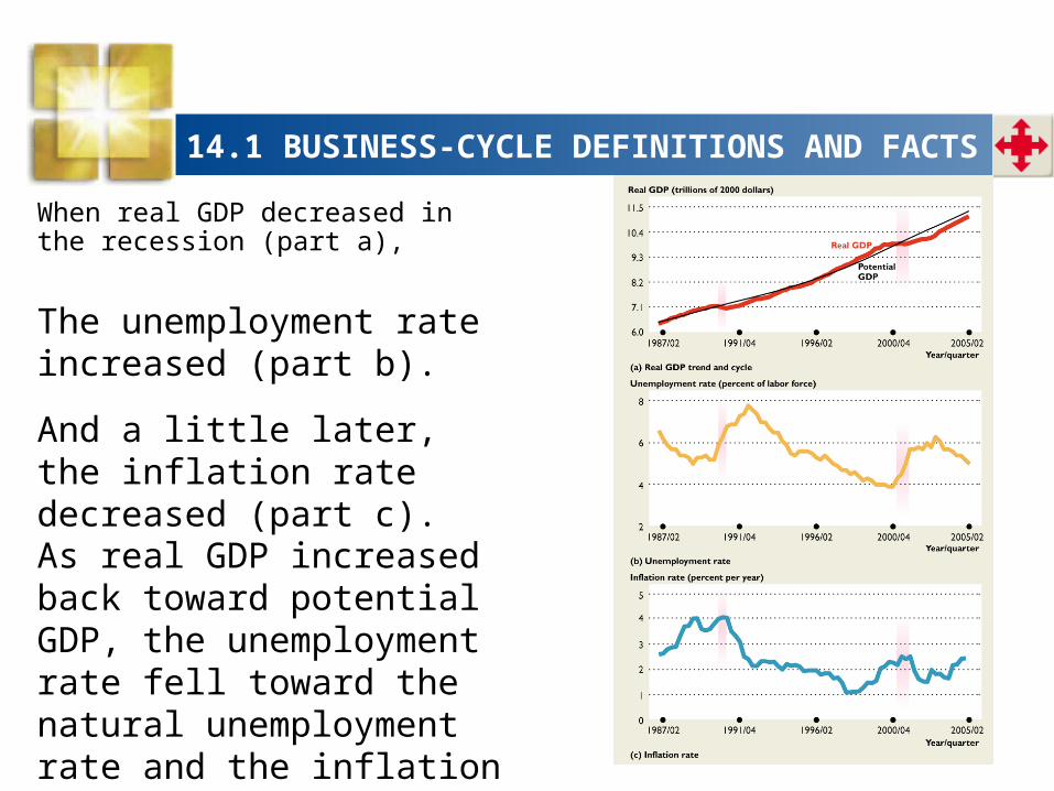
When real GDP decreased in the recession (part a),
The unemployment rate increased (part b).
And a little later, the inflation rate decreased (part c).
As real GDP increased back toward potential GDP, the unemployment rate fell toward the natural unemployment rate and the inflation rate fell.
14.2 AGGREGATE SUPPLY
Real GDP depends on the quantities of• Labor employed• Capital, human capital, and the state of
technology• Land and natural resources• Entrepreneurial talent
14.2 AGGREGATE SUPPLY
At full employment:• The real wage rate makes the quantity of labor
demanded equal to the quantity of labor supplied.• Real GDP equals potential GDP.
Over the business cycle:• The quantity of labor employed fluctuates around
its full employment level.• Real GDP fluctuates around potential GDP.
14.2 AGGREGATE SUPPLY
Aggregate Supply Basics
Aggregate supply is the relationship between the quantity of real GDP supplied and the price level when all other influences on production plans remain the same.
Other things remaining the same,• When the price level rises, the quantity of real
GDP supplied increases.• When the price level falls, the quantity of real GDP
supplied decreases.
14.2 AGGREGATE SUPPLY
Along the aggregate supply curve, the only influence on production plans that changes is the price level.
All the other influences on production plans remain constant. Among these other influences are
• The money wage rate• The money prices of other resources
In contrast, along the potential GDP line, when the price level changes the money wage rate changes to keep the real wage rate at the full-employment level.
14.2 AGGREGATE SUPPLY
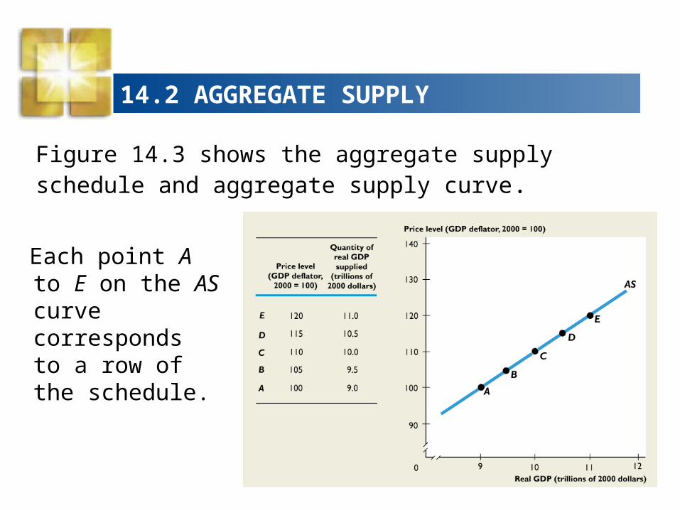
Figure 14.3 shows the aggregate supply schedule and aggregate supply curve.
Each point A to E on the AS curve corresponds to a row of the schedule.
14.2 AGGREGATE SUPPLY
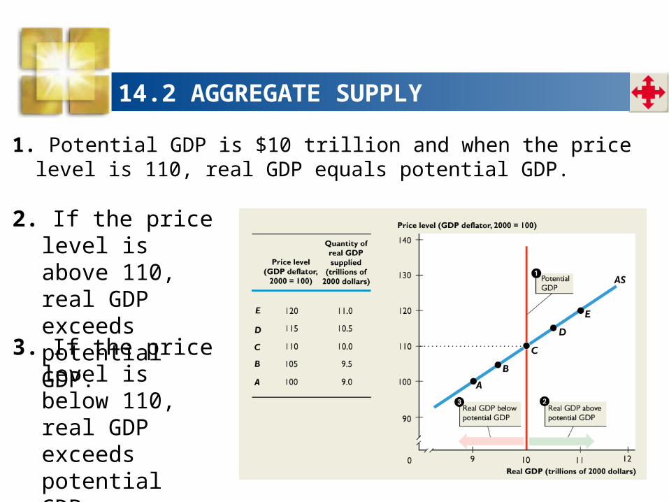
1. Potential GDP is $10 trillion and when the price level is 110, real GDP equals potential GDP.
2. If the price level is above 110, real GDP exceeds potential GDP.
3. If the price level is below 110, real GDP exceeds potential GDP.
14.2 AGGREGATE SUPPLY
Why the AS Curve Slopes Upward
When the price level rises and the money wage rate is constant, the real wage rate falls and employment increases. The quantity of real GDP supplied increases.
When the price level falls and the money wage rate is constant, the real wage rate rises and employment decreases. The quantity of real GDP supplied decreases.
14.2 AGGREGATE SUPPLY
Changes in Aggregate Supply
Aggregate supply changes when any influence on production plans other than the price level changes.
In particular, aggregate supply changes when• Potential GDP changes.• The money wage rate changes.• The money prices of other resources change.
14.2 AGGREGATE SUPPLY
Changes in Potential GDP
Anything that changes potential GDP changes aggregate supply and shifts the aggregate supply curve.
Figure 14.4 on the next slide illustrates.
14.2 AGGREGATE SUPPLY
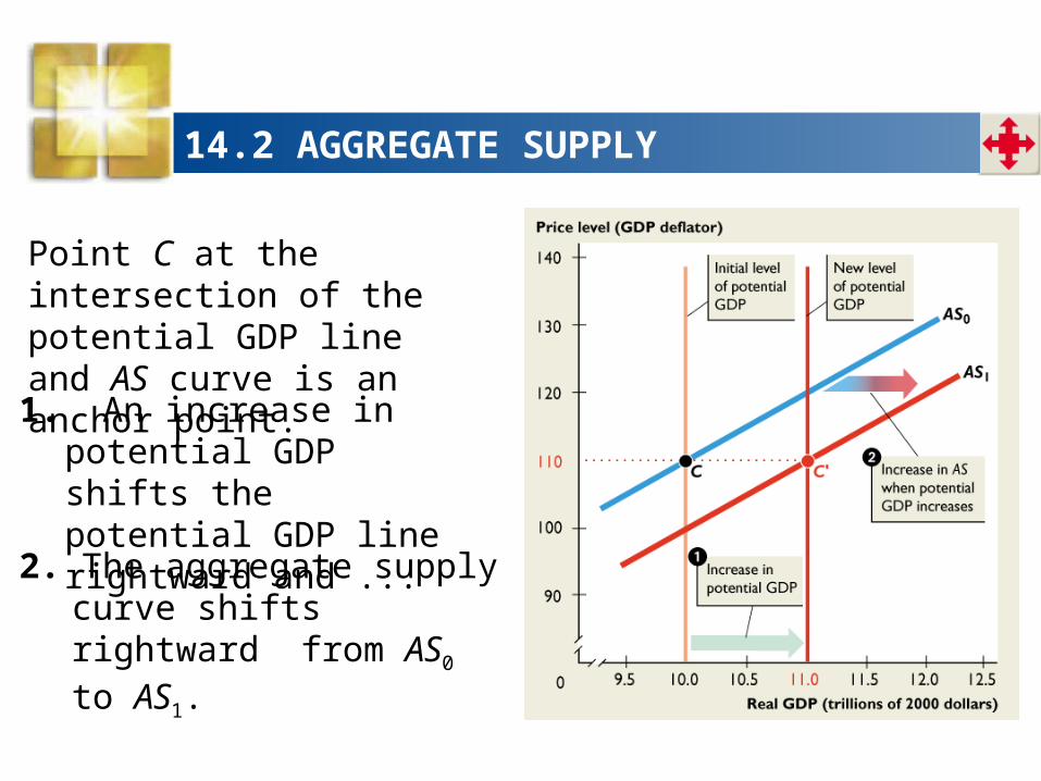
1. An increase in potential GDP shifts the potential GDP line rightward and ...
2. The aggregate supply curve shifts rightward from AS0 to AS1.
Point C at the intersection of the potential GDP line and AS curve is an anchor point.
14.2 AGGREGATE SUPPLY
Changes in Money Wages and Other Resource Prices
A change in the money wage rate or the money price of another resource changes aggregate supply because it changes firms’ costs.
The higher the money wage rate, the higher are firms’ costs and the smaller is the quantity that firms are willing to supply at each price level.
So an increase in the money wage rate decreases aggregate supply.
14.2 AGGREGATE SUPPLY
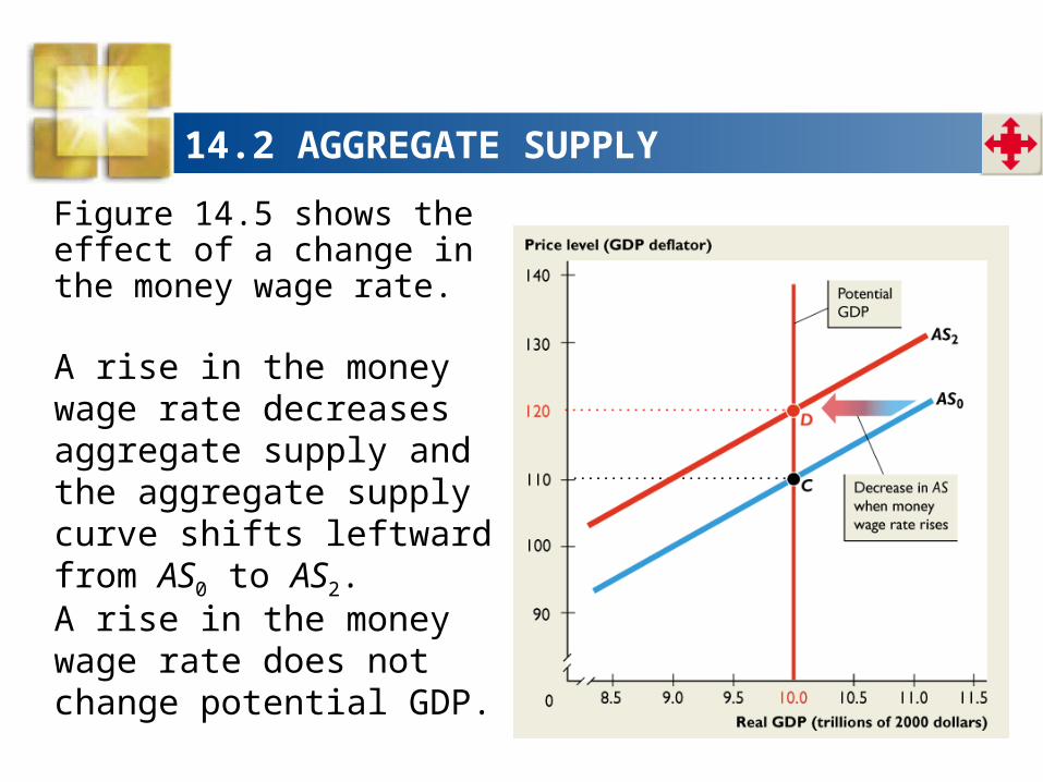
Figure 14.5 shows the effect of a change in the money wage rate.
A rise in the money wage rate decreases aggregate supply and the aggregate supply curve shifts leftward from AS0 to AS2.
A rise in the money wage rate does not change potential GDP.
14.3 AGGREGATE DEMAND
The quantity of real GDP demanded is the total amount of final goods and services produced in the United States that people, businesses, governments, and foreigners plan to buy.
This quantity is the sum of the real consumption expenditure (C), investment (I), government expenditure on goods and services (G), and exports (X) minus imports (M).
That is,
Y = C + I + G + X – M
14.3 AGGREGATE DEMAND
Aggregate Demand Basics
Aggregate demand is the relationship between the quantity of real GDP demanded and the price level when all other influences on expenditure plans remain the same.
Other things remaining the same,
• When the price level rises, the quantity of real GDP demanded decreases.
• When the price level falls, the quantity of real GDP demanded increases.
14.3 AGGREGATE DEMAND
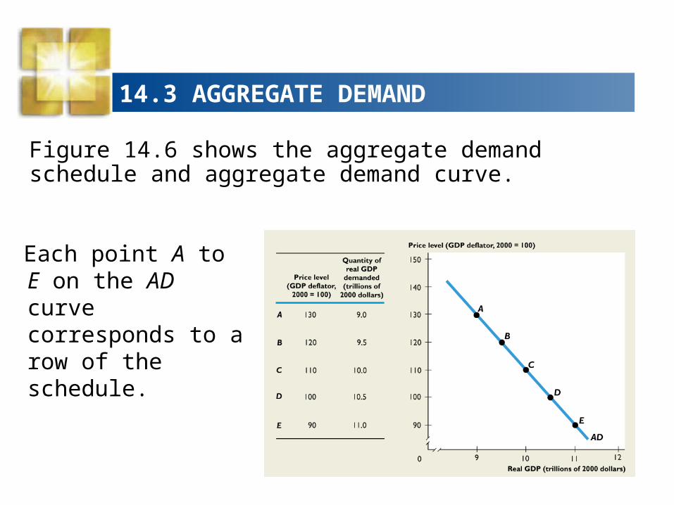
Figure 14.6 shows the aggregate demand schedule and aggregate demand curve.
Each point A to E on the AD curve corresponds to a row of the schedule.
14.3 AGGREGATE DEMAND
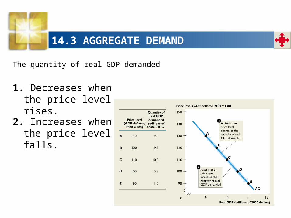
The quantity of real GDP demanded
2. Increases when the price level falls.
1. Decreases when the price level rises.
14.3 AGGREGATE DEMAND
The price level influences the quantity of real GDP demanded because a change in the price level brings changes in
• The buying power of money• The real interest rate• The real prices of exports and imports
14.3 AGGREGATE DEMAND
The Buying Power of Money
A rise in the price level lowers the buying power of money and decreases the quantity of real GDP demanded.
For example, if the price level rises and other things remain the same, a given quantity of money will buy less goods and services, so people cut their spending.
So the quantity of real GDP demanded decreases.
14.3 AGGREGATE DEMAND
The Real Interest Rate
When the price level rises, the real interest rate rises.
An increase in the price level increases the amount of money that people want to hold—increases the demand for money.
When the demand for money increases, the nominal interest rate rises.
In the short run, the inflation rate doesn’t change, so a rise in the nominal interest rate brings a rise in the real interest rate.
14.3 AGGREGATE DEMAND
Faced with a higher real interest rate, businesses and people delay plans to buy new capital goods and consumer durable goods and cut back on spending.
So the quantity of real GDP demanded decreases.
14.3 AGGREGATE DEMAND
The Real Prices of Exports and Imports
When the U.S. price level rises and other things remain the same, the prices in other countries do not change.
So a rise in the U.S. price level makes U.S.-made goods and services more expensive relative to foreign-made goods and services.
This change in real prices encourages people to spend less on U.S.-made items and more on foreign-made items.
14.3 AGGREGATE DEMAND
In the long run, when the price level changes by more in one country than in other countries, the exchange rate changes.
The exchange rate neutralizes the price level change, so this international price effect on buying plans is a short-run effect only.
But the short-run effect is powerful.
14.3 AGGREGATE DEMAND
Changes in Aggregate Demand
A change in any factor that influences expenditure plans other than the price level brings a change in aggregate demand.
• When aggregate demand increases, the aggregate demand curve shifts rightward.
• When aggregate demand decreases, the aggregate demand curve shifts leftward.
14.3 AGGREGATE DEMAND
The factors that change aggregate demand are• Expectations about the future• Fiscal policy and monetary policy• The state of the world economy
14.3 AGGREGATE DEMAND
Expectations
An increase in expected future income increases the amount of consumption goods that people plan to buy today and increases aggregate demand.
An increase in expected future inflation increases aggregate demand today because people decide to buy more goods and services now before their prices rise.
An increase in expected future profit increases the investment that firms plan to undertake today and increases aggregate demand.
14.3 AGGREGATE DEMAND
Fiscal Policy and Monetary Policy
Government can influence aggregate demand by set-ting and changing taxes, transfer payments, and government expenditure on goods and services.
The Federal Reserve can influence aggregate demand by changing the quantity of money and the interest rate.
14.3 AGGREGATE DEMAND
A tax cut or an increase in either transfer payments or government expenditure on goods and services increases aggregate demand.
A cut in the interest rate or an increase in the quantity of money increases aggregate demand.
14.3 AGGREGATE DEMAND
The World Economy
The foreign exchange rate and foreign income influence aggregate demand.
Foreign exchange rate is the amount of foreign currency you can buy with a U.S. dollar.
Other things remaining the same, a rise in the foreign exchange rate decreases aggregate demand.
An increase in foreign income increases U.S. exports and increases U.S. aggregate demand.
14.3 AGGREGATE DEMAND
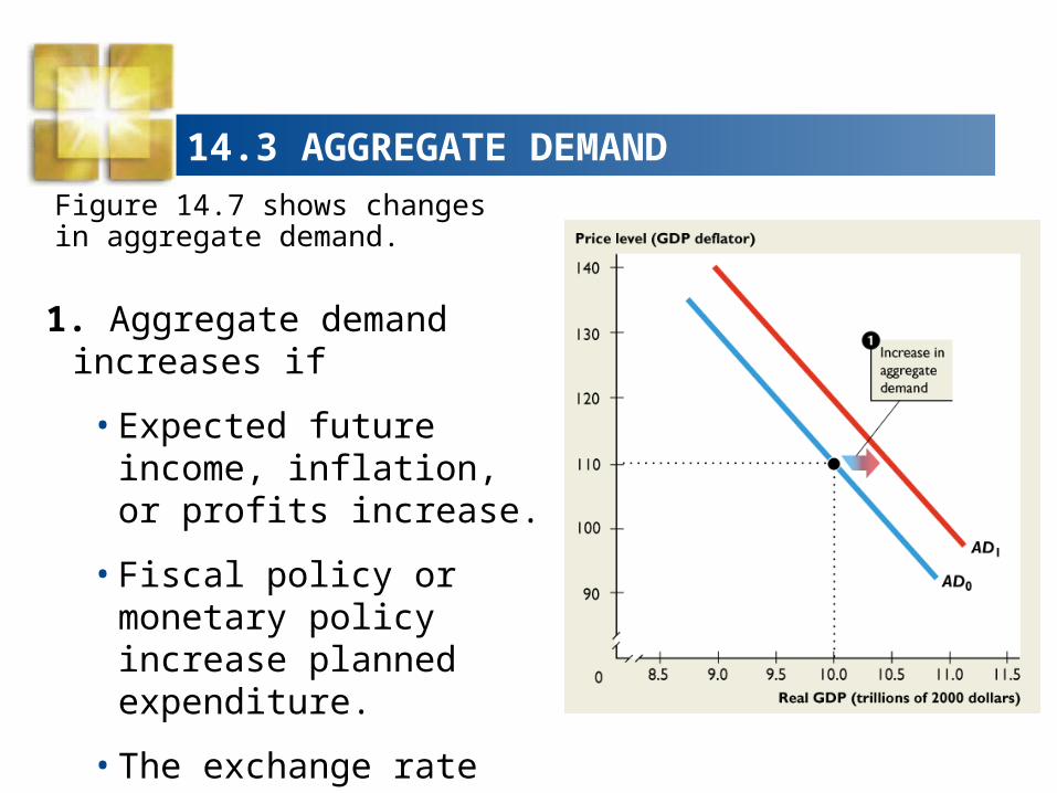
Figure 14.7 shows changes in aggregate demand.
1. Aggregate demand increases if
• Expected future income, inflation, or profits increase.
• Fiscal policy or monetary policy increase planned expenditure.
• The exchange rate falls or foreign income increases.
14.3 AGGREGATE DEMAND
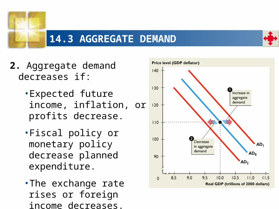
2. Aggregate demand decreases if:
• Expected future income, inflation, or profits decrease.
• Fiscal policy or monetary policy decrease planned expenditure.
• The exchange rate rises or foreign income decreases.
14.3 AGGREGATE DEMAND
The Aggregate Demand Multiplier
The aggregate demand multiplier is an effect that magnifies changes in expenditure plans and brings potentially large fluctuations in aggregate demand.
When any influence on aggregate demand changes expenditure plans:
• The change in expenditure changes income.• And the change in income induces a change in
consumption expenditure.
14.3 AGGREGATE DEMAND
• The increase in aggregate demand is the initial increase in expenditure plus the induced increase in consumption expenditure.
14.3 AGGREGATE DEMAND
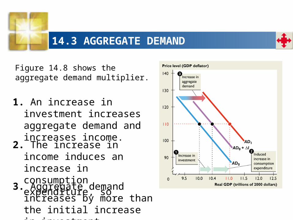
Figure 14.8 shows the aggregate demand multiplier.
1. An increase in investment increases aggregate demand and increases income.
2..The increase in income induces an increase in consumption expenditure, so
3. Aggregate demand increases by more than the initial increase in investment.
14.4 UNDERSTANDING BUSINESS CYCLES
Aggregate supply and aggregate demand determine real GDP and the price level.
Macroeconomic equilibrium occurs when the quantity of real GDP demanded equals the quantity of real GDP supplied at the point of intersection of the AD curve and the AS curve.
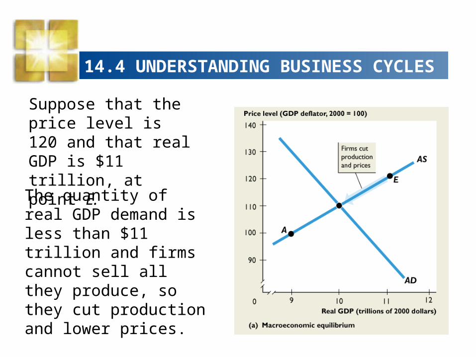
Figure 14.9(a) on the next slide illustrates macroeconomic equilibrium.
14.4 UNDERSTANDING BUSINESS CYCLES
The quantity of real GDP demand is less than $11 trillion and firms cannot sell all they produce, so they cut production and lower prices.
Suppose that the price level is 120 and that real GDP is $11 trillion, at point E.
14.4 UNDERSTANDING BUSINESS CYCLES
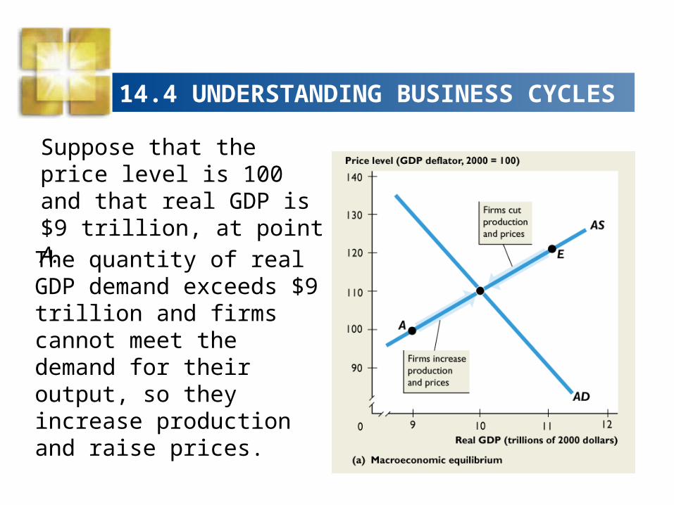
The quantity of real GDP demand exceeds $9 trillion and firms cannot meet the demand for their output, so they increase production and raise prices.
Suppose that the price level is 100 and that real GDP is $9 trillion, at point A.
14.4 UNDERSTANDING BUSINESS CYCLES
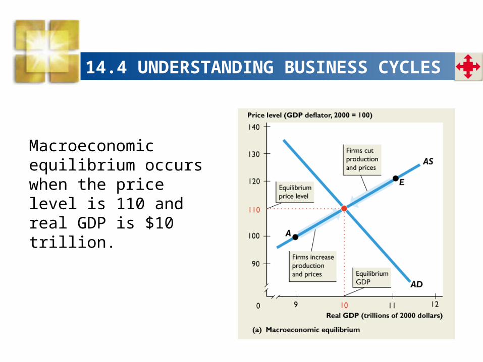
Macroeconomic equilibrium occurs when the price level is 110 and real GDP is $10 trillion.
14.4 UNDERSTANDING BUSINESS CYCLES
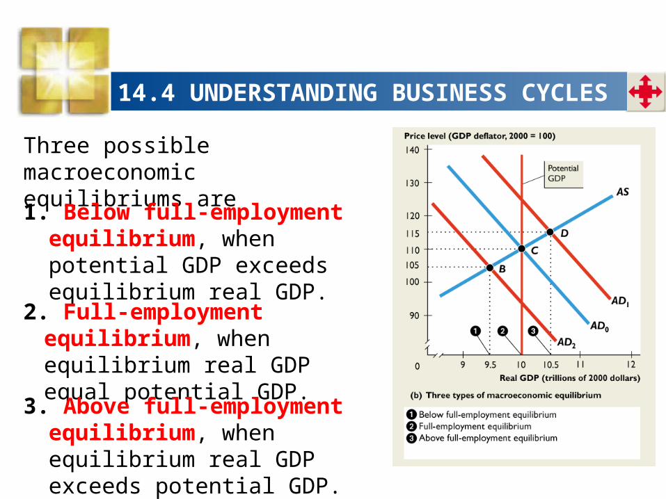
Three possible macroeconomic equilibriums are
1. Below full-employment equilibrium, when potential GDP exceeds equilibrium real GDP.
2. Full-employment equilibrium, when equilibrium real GDP equal potential GDP.
3. Above full-employment equilibrium, when equilibrium real GDP exceeds potential GDP.
14.4 UNDERSTANDING BUSINESS CYCLES
Aggregate Demand Fluctuations
Fluctuations in aggregate demand are one of the sources of the business cycle.
To focus on the business cycle, we’ll ignore economic growth and inflation and suppose that potential GDP and the full-employment price level is constant.
Figure 14.10 in the next slide illustrates the business cycle.
14.4 UNDERSTANDING BUSINESS CYCLES
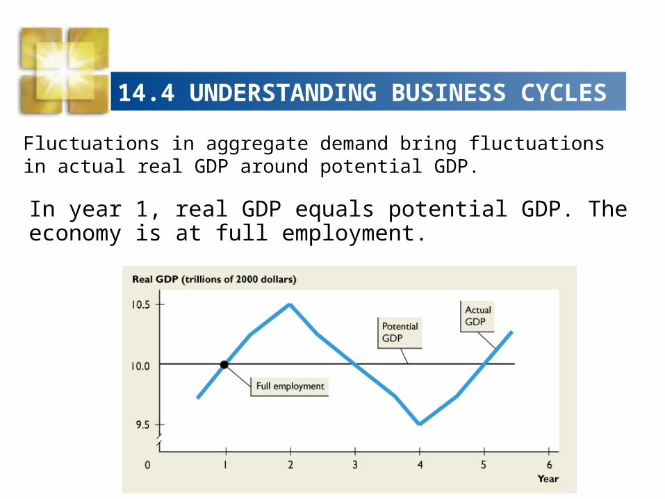
Fluctuations in aggregate demand bring fluctuations in actual real GDP around potential GDP.
In year 1, real GDP equals potential GDP. The economy is at full employment.
14.4 UNDERSTANDING BUSINESS CYCLES
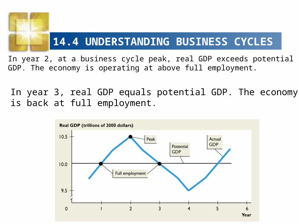
In year 2, at a business cycle peak, real GDP exceeds potential GDP. The economy is operating at above full employment.
In year 3, real GDP equals potential GDP. The economy is back at full employment.
14.4 UNDERSTANDING BUSINESS CYCLES
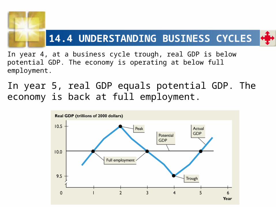
In year 4, at a business cycle trough, real GDP is below potential GDP. The economy is operating at below full employment.
In year 5, real GDP equals potential GDP. The economy is back at full employment.
14.4 UNDERSTANDING BUSINESS CYCLES
Aggregate Supply Fluctuations
Aggregate supply fluctuates for two types of reasons:• Potential GDP grows at an uneven pace. • The money price of a major resource, such as
crude oil, might change.
Stagflation
A combination of recession (falling real GDP) and inflation (rising price level).
14.4 UNDERSTANDING BUSINESS CYCLES
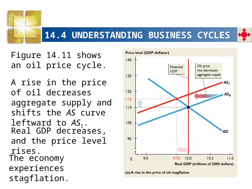
Figure 14.11 shows an oil price cycle.
A rise in the price of oil decreases aggregate supply and shifts the AS curve leftward to AS1.
Real GDP decreases, and the price level rises.
The economy experiences stagflation.
14.4 UNDERSTANDING BUSINESS CYCLES
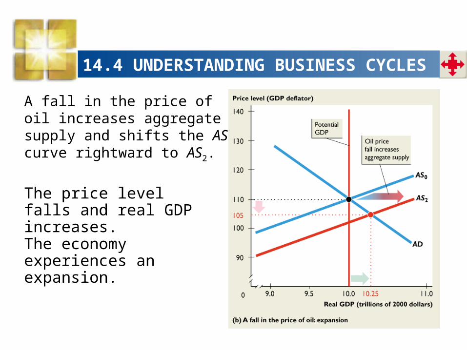
A fall in the price of oil increases aggregate supply and shifts the AS curve rightward to AS2.
The price level falls and real GDP increases.
The economy experiences an expansion.
14.4 UNDERSTANDING BUSINESS CYCLES
Adjustment Toward Full Employment
When the economy is away from full employment, forces operate to restore full employment.
Inflationary gap
A gap that exists when real GDP exceeds potential GDP and that brings a rising price level.
Recessionary gap
A gap that exists when potential GDP exceeds real GDP and that brings a falling price level.
14.4 UNDERSTANDING BUSINESS CYCLES
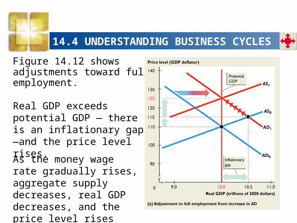
Figure 14.12 shows adjustments toward full employment.
Real GDP exceeds potential GDP — there is an inflationary gap —and the price level rises.
As the money wage rate gradually rises, aggregate supply decreases, real GDP decreases, and the price level rises farther.
14.4 UNDERSTANDING BUSINESS CYCLES
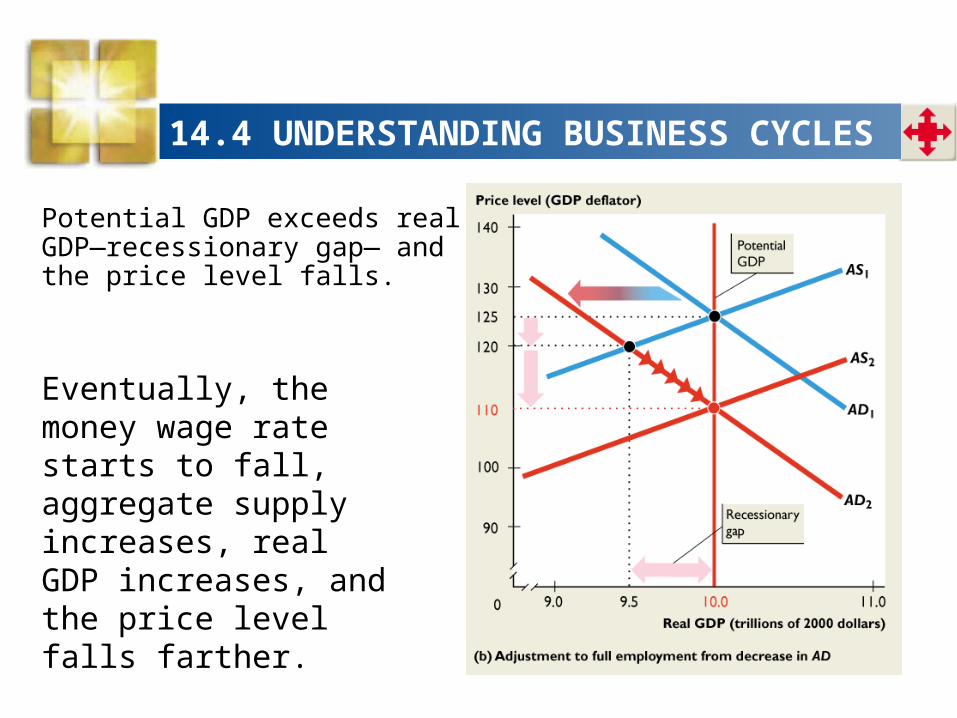
Potential GDP exceeds real GDP—recessionary gap— and the price level falls.
Eventually, the money wage rate starts to fall, aggregate supply increases, real GDP increases, and the price level falls farther.

AS-AD in YOUR Life
Consider the U.S. economy right now.
Using the knowledge you have accumulated over the course and information you have read in the current news, do you think real GDP is currently above, below, or at potential GDP?
Talk to your class mates about where they see the U.S. economy right now. Is there a consensus?
What are the main pressures on AS and AD right now?
Do you think that real GDP will expand more quickly or more slowly over the coming months?
Will the gap between real GDP and potential GDP widen or narrow?


