Part-I … Comparative Study and Improvement in Shallow Water Model. Dr. Rajendra K. Ray. Assistant Professor, School of Basic Sciences, Indian Institute of Technology Mandi, Mandi-175001, H.P., India. Collaborators: Prof. Kim Dan Nguyen & Dr. Yu-e Shi. - PowerPoint PPT Presentation
Part-I … Comparative Study and Improvement in Shallow Water Model Collaborators: Prof. Kim Dan Nguyen & Dr. Yu-e Shi Speaker: Dr. Rajendra K. Ray Date: 16. 09. 2014 Assistant Professor, School of Basic Sciences, Indian Institute of Technology Mandi, Mandi-175001, H.P., India Dr. Rajendra K. Ray
Transcript
Part-I …Comparative Study and
Improvement in Shallow Water Model
Collaborators: Prof. Kim Dan Nguyen & Dr. Yu-e Shi
Speaker: Dr. Rajendra K. Ray Date: 16. 09. 2014
Assistant Professor,School of Basic Sciences,
Indian Institute of Technology Mandi,Mandi-175001, H.P., India
Dr. Rajendra K. Ray
2
Outlines
Introduction
Governing Equations and projection method
Wetting and drying treatment
Numerical ValidationParabolic Bowl
Application to Malpasset dam-break problem
Conclusion
Dr. Rajendra K. Ray 16.09.2014
3
Introduction
Free-surface water flows occur in many real life flow situations
These types of flow behaviours can be modelled mathematically by Shallow-Water Equations (SWE)
The unstructured finite-volume methods (UFVMs) not
only ensure local mass conservation but also the best possible fitting of computing meshes into the studied domain boundaries
The present work extends the unstructured finite volumes method for moving boundary problems
Many of these flows involve irregular flow domains
with moving boundaries
Dr. Rajendra K. Ray 16.09.2014
4
Governing Equations and projection method
Shallow Water Equations:
Continuity Equation
)1(0
y
hv
x
hu
t
Z s
Momentam Equations
)2(
2
o
bxHH
s
y
huA
yx
huA
xx
Zghhvf
y
huv
x
hu
t
hu
)3(
2
o
byHH
s
y
hvA
yx
hvA
xy
Zghhuf
y
hv
x
huv
t
hv
Dr. Rajendra K. Ray 16.09.2014
5
Governing Equations and projection method …
Projection Method:
Convection-diffusion step
)4(
2
*2
2
*2***
2
*2
2
*2***
y
q
x
qA
y
vq
x
uq
t
q
y
q
x
qA
y
vq
x
uq
t
q
yyH
yyy
xxH
xxx
Wave propagation step
)5(1 12
2
2
22ns
nsss ZZZwhere
A
BZ
yxA
gh
)6(
,,,
1
22
2211
**
2
2
2
2
wyy
wxx
ny
nx
h
ny
nxyxyx
ns
ns
LLqqhC
gFFdtdtA
y
q
x
q
dty
L
x
L
y
q
x
q
dty
Z
x
ZghB
Dr. Rajendra K. Ray 16.09.2014
6
Governing Equations and projection method …
Velocity correction step
)7(11)1( 11
*1
FdtdtFqdtL
x
Zghdt
x
Zghdtqq n
xx
ns
ns
xnx
Equations (4)-(8) have been integrated by a technique based on Green’s theorem and then discretised by an Unstructured Finite-Volume Method (UFVM).
)8(11)1( 11
*1
FdtdtFqdtL
y
Zghdt
y
Zghdtqq n
yy
ns
ns
yny
The convection terms are handled by a 2nd order Upwind Least Square Scheme (ULSS) along with the Local Extremum Diminishing (LED) technique to preserve the monotonicity of the scalar veriable
The linear equation system issued from the wave propagation step is implicitly solved by a Successive Over Relaxation (SOR) technique.
Dr. Rajendra K. Ray 16.09.2014
7
Steady wetting/drying fronts over adverse steep slopes in real and discrete representations
Dr. Rajendra K. Ray 16.09.2014
8
Modification of the bed slope in steady wetting/drying fronts over adverse steep slopes in real and discrete representations
Dr. Rajendra K. Ray 16.09.2014
9
Wetting and drying treatment
The main idea is to find out the partially drying or flooding cells in each time step and then add or subtract hypothetical fluid mass to fill the cell or to make the cell totally dry respectively, and then subtract or add the same amount of fluid mass to the neighbouring wet cells in the computational domain [Brufau et. al. (2002)].
To consider a cell to be wet or dry in an particular time step, we use the threshold value as the minimum water depth (h) )10( 3O
If the cell will be considered as dry and the water depth for that cell set to be fixed as for that time step
,hh
Dr. Rajendra K. Ray 16.09.2014
10
Conservative Property
Definition: If a numerical scheme can produce the exact solution to the still
water case: )(,0, IVHZ s
then the scheme is said to satisfy the Conservative Property (C-property)
[Bermudez and Vázquez 1994].
Proposition 1. The present numerical scheme satisfies the C-property.
Proof. The details of the proof can be found in Shi et at. 2013 (Comp & Fluids).
Dr. Rajendra K. Ray 16.09.2014
11
Numerical Validation
To test the capacity of the present model in describing the wetting and drying transition
Parabolic Bowl :
The bed topography of the domain is defined by , where is a positive constant and
2b(x) r 222 yxr
The water depth is non-zero for ),( trh)(
)cos(22 YX
tYXr
The analytical solution is periodic in time with a period 2
The analytical solution is given within the range as
,coscos
1),( 2
222
tYX
rXY
tYXtrh
.2,2cos
sin,,
yx
tYX
tYtxvu
Dr. Rajendra K. Ray 16.09.2014
12
Numerical Validation …
Parabolic Bowl …
For computation purpose, , and are fixed as , and respectively
X Y 17106.1 m 11 m141884.0 m
The computational domain ( ) is considered as a square region
with the origin at the domain centre
2]4000,4000[]4000,4000[ m
The threshold value is set as 3103
Dr. Rajendra K. Ray 16.09.2014
13
Numerical Validation …
Parabolic Bowl …
6/t 6/2t 6/3t
6/4t 6/5t t
Dr. Rajendra K. Ray 16.09.2014
14
Numerical Validation …
Parabolic Bowl …6/t 6/2t 6/3t
6/4t 6/5t t
Dr. Rajendra K. Ray 16.09.2014
15
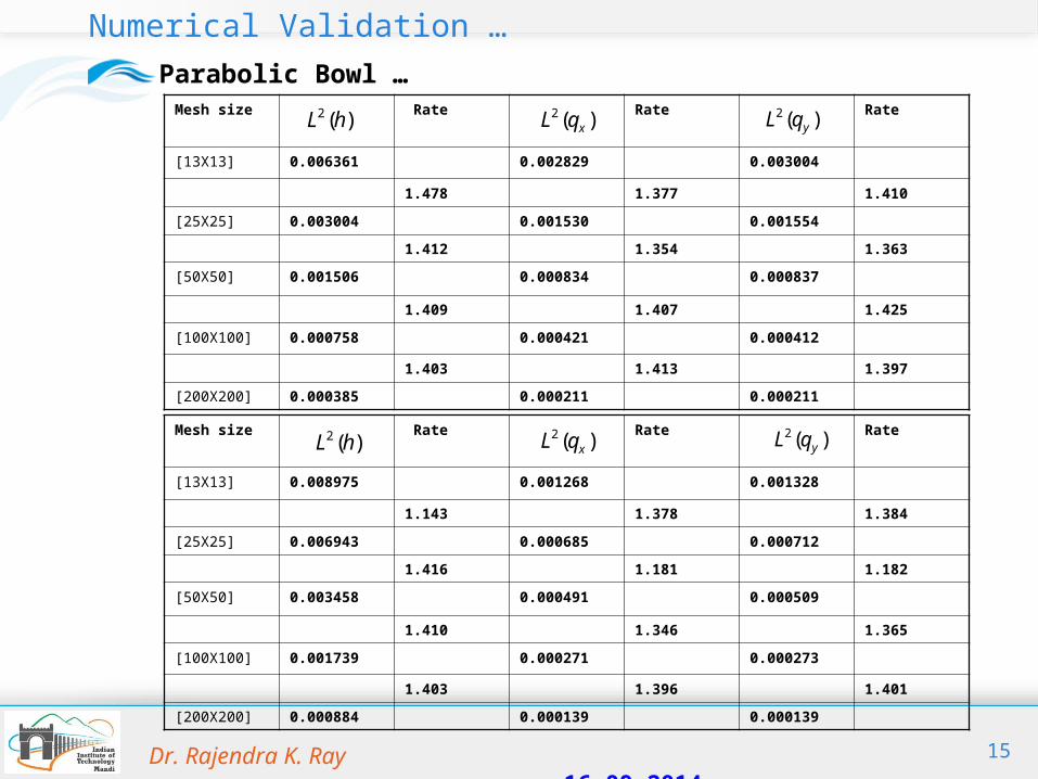
Numerical Validation …
Parabolic Bowl …Mesh size Rate Rate Rate
[13X13] 0.006361 0.002829 0.003004
1.478 1.377 1.410
[25X25] 0.003004 0.001530 0.001554
1.412 1.354 1.363
[50X50] 0.001506 0.000834 0.000837
1.409 1.407 1.425
[100X100] 0.000758 0.000421 0.000412
1.403 1.413 1.397
[200X200] 0.000385 0.000211 0.000211
)(2 hL )(2xqL )(2
yqL
Mesh size Rate Rate Rate
[13X13] 0.008975 0.001268 0.001328
1.143 1.378 1.384
[25X25] 0.006943 0.000685 0.000712
1.416 1.181 1.182
[50X50] 0.003458 0.000491 0.000509
1.410 1.346 1.365
[100X100] 0.001739 0.000271 0.000273
1.403 1.396 1.401
[200X200] 0.000884 0.000139 0.000139
)(2 hL )(2xqL )(2
yqL
Dr. Rajendra K. Ray 16.09.2014
16
Numerical Validation …
Parabolic Bowl …
Average Rate of convergence
Average Rate of convergence
Bunya et. al. (2009)
1.33 0.84
Ern et. al. (2008)
1.4 0.5
Present
1.4 1.4
)2/( t )( t
Relative error in global mass conservation is less than 0.003%
Dr. Rajendra K. Ray 16.09.2014
17
Application to the Dam-Break of Malpasset
Back Grounds
The generated flood wave swept across the downstream part of Reyran valley modifying its morphology and destroying civil works such as bridges and a portion of the highway
The Malpasset Dam was located at a narrow gorge of the Reyran River valley (French Riviera) with water storage of 361055 m
It was explosively broken at 9:14 p.m. on December 2, 1959 following an exceptionally heavy rain
The flood water level rose to a level as high as 20 m above the original bed level
After this accident, a field survey was done by the local police
In addition, a physical model was built to study the dam-break flow in 1964
Dr. Rajendra K. Ray 16.09.2014
18
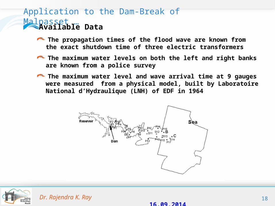
Application to the Dam-Break of Malpasset …
The propagation times of the flood wave are known from the exact shutdown time of three electric transformers
The maximum water levels on both the left and right banks are known from a police survey
The maximum water level and wave arrival time at 9 gauges were measured from a physical model, built by Laboratoire National d’Hydraulique (LNH) of EDF in 1964
Available Data
Dr. Rajendra K. Ray 16.09.2014
19
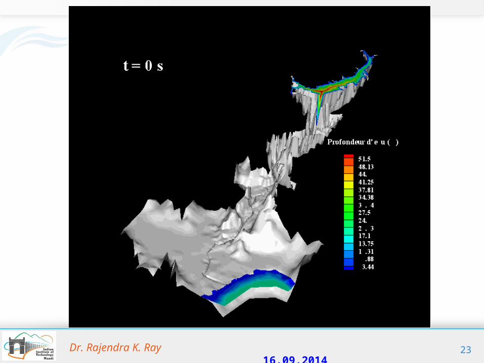
Application to the Dam-Break of Malpasset …
Results and Discussions
Water depth and velocity field at t =1000 s Water depth at t =2400 s, wave front reaching sea
Dr. Rajendra K. Ray 16.09.2014
20
Application to the Dam-Break of Malpasset …
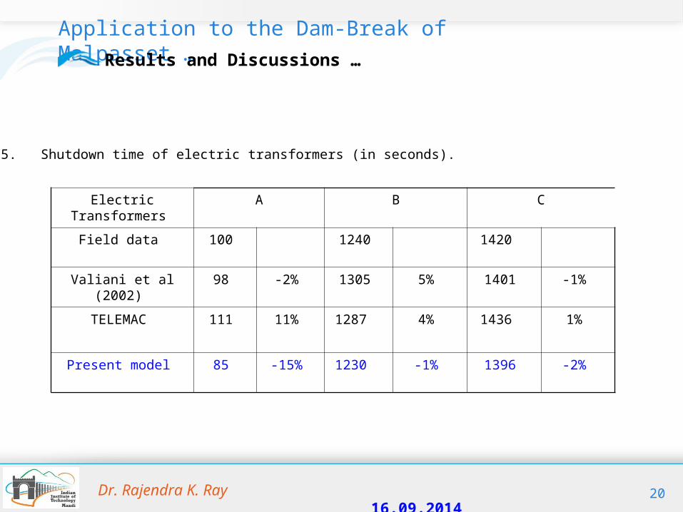
Results and Discussions …
Electric Transformers A B C
Field data 100 1240 1420
Valiani et al (2002) 98 -2% 1305 5% 1401 -1%
TELEMAC 111 11% 1287 4% 1436 1%
Present model 85 -15% 1230 -1% 1396 -2%
Table 5. Shutdown time of electric transformers (in seconds).
Dr. Rajendra K. Ray 16.09.2014
21
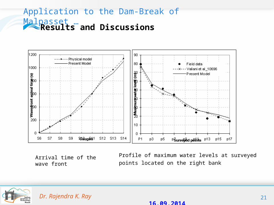
Application to the Dam-Break of Malpasset …
Results and Discussions
Arrival time of the wave front Profile of maximum water levels at surveyed
points located on the right bank
Dr. Rajendra K. Ray 16.09.2014
22
Application to the Dam-Break of Malpasset …
Results and Discussions
maximum water levels at surveyed points
located on the left bank
Maximum water level
Dr. Rajendra K. Ray 16.09.2014
23Dr. Rajendra K. Ray 16.09.2014
24
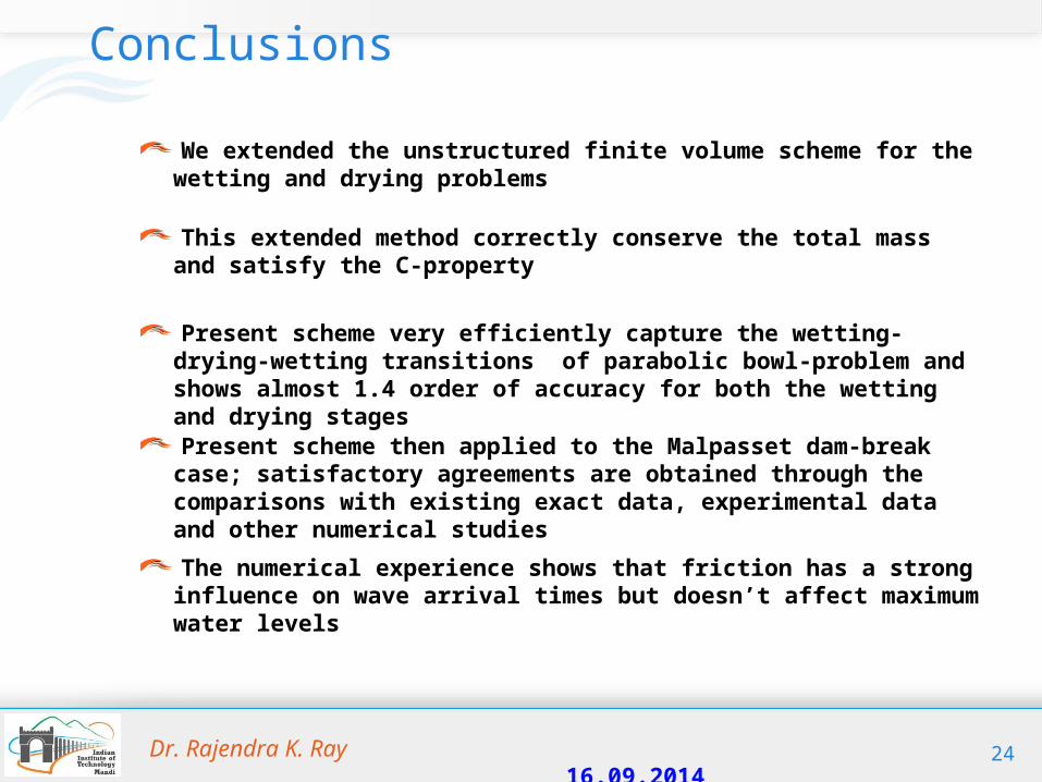
Conclusions
We extended the unstructured finite volume scheme for the wetting and drying problems
This extended method correctly conserve the total mass and satisfy the C-property
Present scheme very efficiently capture the wetting-drying-wetting transitions of parabolic bowl-problem and shows almost 1.4 order of accuracy for both the wetting and drying stages
The numerical experience shows that friction has a strong influence on wave arrival times but doesn’t affect maximum water levels
Present scheme then applied to the Malpasset dam-break case; satisfactory agreements are obtained through the comparisons with existing exact data, experimental data and other numerical studies
Dr. Rajendra K. Ray 16.09.2014
25
References
Nguyen K.D., Shi Y., Wang S.S.Y., Nguyen T.H., 2006. 2D Shallow-Water Model Using Unstructured Finite-Volumes Methods. J. Hydr Engrg., ASCE, 132(3), p. 258–269 .
Bermudez A., Vázquez M.E., 1994. Upwind Methods for Hyperbolic Conservation Laws with Source Terms. Comput. Fluids, 23, p. 1049–1071.
Ern A., Piperno S., Djadel K., 2008. A well-balanced Runge–Kutta discontinuous Galerkin method for the shallow-water equations with flooding and drying. Int. J. Numer. Meth. Fluids, 58, p. 1–25.
Valiani A., Caleffi V., Zanni A., 2002. Case study: Malpasset dam-break simulation using a two-dimensional finite volume method. J. Hydraul. Eng., 128(5), 460–472.
Technical Report HE-43/97/016A, 1997. Electricité de France, Département Laboratoire National d’Hydraulique, groupe Hydraulique Fluviale.
Brufau P., Vázquez-Cendón M.E., García-Navarro, P., 2002. A Numerical Model for the Flooding and Drying of Irregular Domains. Int. J. Numer. Meth. Fluids, 39, p. 247–275.
Hervouet J.M., 2007. Hydrodynamics of free surface flows-Modelling with the finite element method, John Willey & sons, ISBN 978-0-470-03558-0, 341 p.
Shi Y., Ray R. K., Nguyen K.D., 2013. A projection method-based model with the exact C-property for shallow-water flows over dry and irregular bottom using unstructured finite-volume technique. Comput. Fluids, 76, p. 178–195.
Dr. Rajendra K. Ray 16.09.2014
Part-II …Two-Phase modelling of
sediment transport in the Gironde Estuary (France)
Collaborators: Prof. K. D. Nguyen, Dr. D. Pham Van Bang & Dr. F. Levy
Speaker: Dr. Rajendra K. Ray Date: 16. 09. 2014
Assistant Professor,School of Basic Sciences,
Indian Institute of Technology Mandi,Mandi-175001, H.P., India
Dr. Rajendra K. Ray
27
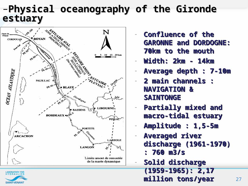
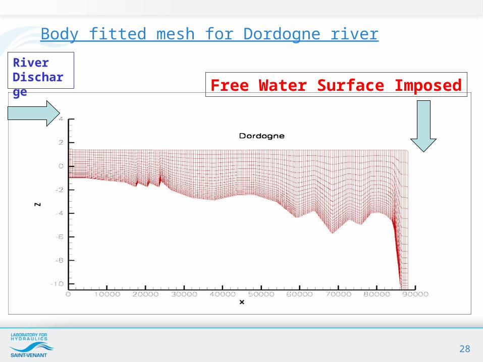
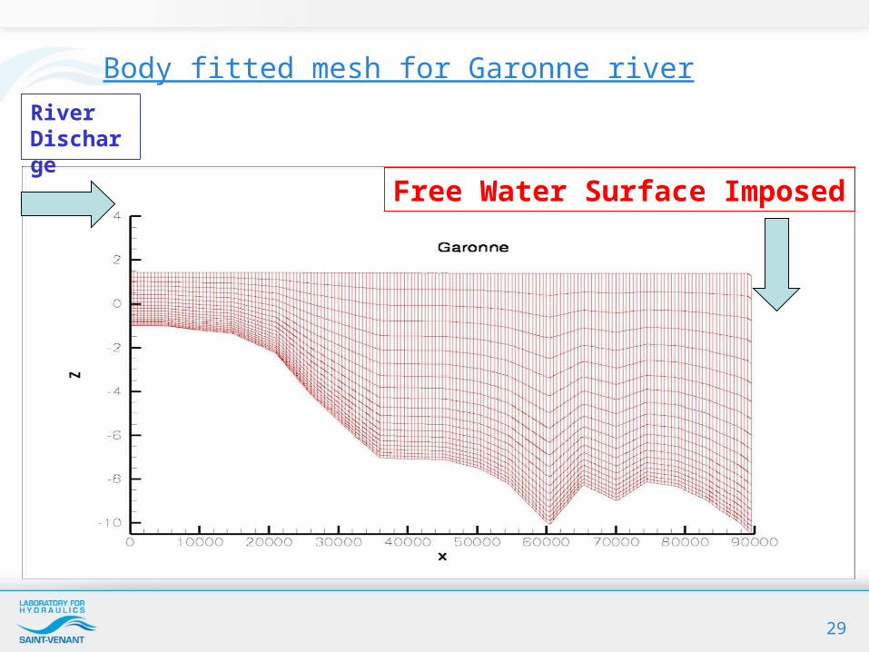
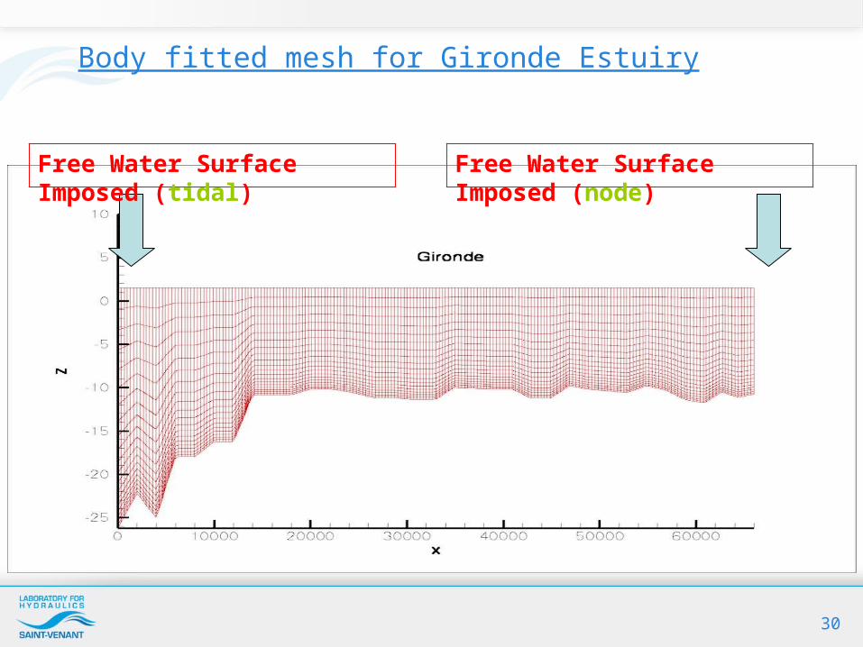
–Physical oceanography of the Gironde Physical oceanography of the Gironde estuaryestuary
- Confluence of the Confluence of the GARONNE and GARONNE and DORDOGNE: 70km to DORDOGNE: 70km to the mouththe mouth