Part II Methods for Independent...

5/20/2014

1

Part II

Methods for

Independent Demand

Chapter 3

Economic Order Quantity

5/20/2014

2

Introduction

• This chapter introduces some quantitative models for

inventory control.

• The first model takes an idealized stock and finds the fixed

order size that minimizes costs.

• This is the economic order quantity (EOQ), which is the

basis of most independent demand methods.

Defining the EOQ:

Background

• EOQ was first referenced to the work by Harris (1915), but

the calculation is often credited to Wilson (1934) who

independently duplicated the work and marketed the

results.

5/20/2014

3

Typical Pattern of Stock Level

Time

Stock

level

Replenishment Replenishment

Place

order

Place

order

Stock

out

Replenishment

Assumptions of Basic EOQ Model

• The demand is known exactly, is continuous and is

constant over time;

• All costs are known exactly and do not vary;

• No shortages are allowed;

• Lead time is zero – so a delivery is made as soon as the

order is placed.

5/20/2014

4


Implicit Assumptions:

• We can consider a single item in isolation, so we cannot

save money by substituting other items or grouping several

items into a single order;

• Purchase price and reorder costs do not vary with the

quantity ordered;

• A single delivery is made for each order;

• Replenishment is instantaneous, so that all of an order

arrives in stock at the same time and can be used

immediately.

Constant Demand Assumption

Time

Demand

5/20/2014

5


The assumptions might seem unrealistic,

• All models are simplifications of reality and their aim is to

give useful results rather than be exact representations of

actual circumstances. The EOQ is widely used, and we can

infer that it is accurate enough for many purposes. The

results may not be optimal in the strict mathematical sense,

but they are good approximations and do, at worst, give

useful guidelines.

• This is a basic model that we can extend in many ways.

Stock Level with Fixed Order Size

Time

Stock

level

5/20/2014

6

Variables Used in the Analysis

• Unit cost (UC) is the price charged by the suppliers for one unit of the

item, or the total cost to the organization of acquiring one unit.

• Reorder cost (RC) is the cost of placing a routine order for the item and

might include allowances for drawing-up an order, correspondence,

telephone costs, receiving, use of equipment, expediting, delivery,

quality checks, and so on. If the item is made internally, this might be a

set-up cost.

• Holding cost (HC) is the cost of holding one unit of the item in stock for

one period of time. The usual period for calculating stock costs is a

year.

• Shortage cost (SC) is the cost of having a shortage and not being able

to meet demand from stock. In this analysis we have said that no

shortages are allowed, so SC does not appear (it is effectively so large

that any shortage would be prohibitively expensive).

Decision Variables

• Order quantity (Q) which is the fixed order size that

we always use.

• Cycle time (T) which is the time between two

consecutive replenishments.

Other Variables

• Demand (D) which sets the number of units to be

supplied from stock in a given time period.

5/20/2014

7

Derivation of the EOQ

Standard approach

1. Find the total cost of one stock cycle.

2. Divide this total cost by the cycle length to get a

cost per unit time.

3. Minimize this cost per unit time.

Stock Level with Fixed Order Size

Time

Stock

level

Place order &

receive deliveryPlace order &

receive delivery

T

D

Average

stock

level

Optimal

order sizeQ

𝑄 = 𝐷 × 𝑇

5/20/2014

8


1. Find the total cost of one stock cycle.

𝑇𝑜𝑡𝑎𝑙 𝑐𝑜𝑠𝑡 𝑝𝑒𝑟 𝑐𝑦𝑐𝑙𝑒= 𝑢𝑛𝑖𝑡 𝑐𝑜𝑠𝑡 𝑐𝑜𝑚𝑝𝑜𝑛𝑒𝑛𝑡 + 𝑟𝑒𝑜𝑟𝑑𝑒𝑟 𝑐𝑜𝑠𝑡 𝑐𝑜𝑚𝑝𝑜𝑛𝑒𝑛𝑡+ ℎ𝑜𝑙𝑑𝑖𝑛𝑔 𝑐𝑜𝑠𝑡 𝑐𝑜𝑚𝑝𝑜𝑛𝑒𝑛𝑡

= UC × Q + RC +HC × Q × T

2


2. Divide this total cost by the cycle length to get a

cost per unit time.

𝑇𝑜𝑡𝑎𝑙 𝑐𝑜𝑠𝑡 𝑝𝑒𝑟 𝑢𝑛𝑖𝑡 time =UC × Q

𝑇+

𝑅𝐶

𝑇+HC × Q

2

𝑆𝑖𝑛𝑐𝑒 𝑄 = 𝐷 × 𝑇

𝑇𝐶 = 𝑈𝐶 × 𝐷 +𝑅𝐶 × 𝐷

𝑄+HC × Q

2

5/20/2014

9


For the economic order

quantity, the reorder cost

component equals the

holding

cost component


3. Minimize this cost per unit time.

𝑑(𝑇𝐶)

𝑑(𝑄)= −

𝑅𝐶 × 𝐷

𝑄2+HC

2= 0

Solve for 𝑄𝑜 (EOQ),

𝑄𝑜 =2 × 𝑅𝐶 × 𝐷

𝐻𝐶

5/20/2014

10


Optimal cycle length

𝑇𝑜 =𝑄𝑜𝐷

=2 × 𝑅𝐶

𝐻𝐶 × 𝐷

Optimal cost per unit time

𝑇𝐶𝑜 = 𝑈𝐶 × 𝐷 +𝑅𝐶 × 𝐷

2 × 𝑅𝐶 × 𝐷𝐻𝐶

+HC ×

2 × 𝑅𝐶 × 𝐷𝐻𝐶

2

= 𝑈𝐶 × 𝐷 + 2 × 𝑅𝐶 × 𝐻𝐶 × 𝐷 = 𝑈𝐶 × 𝐷 + 𝐻𝐶 × 𝑄𝑜

Worked Example 1:

EOQ

Jaydeep Company buys 6,000 units of an item every year with a unit

cost of $30. It costs $125 to process an order and arrange delivery,

while interest and storage costs amount to $6 a year for each unit

held. What is the best ordering policy for the item?

𝐷 = 6000 units/yr 𝑅𝐶= $125 an order

𝑈𝐶= $30 a unit 𝐻𝐶= $6/yr for a unit

𝑄𝑜 =2 × 𝑅𝐶 × 𝐷

𝐻𝐶=

2 × 125 × 6000

6= 500


=500

6000=

1

12𝑦𝑒𝑎𝑟 = 1 𝑚𝑜.

𝑇𝐶𝑜 = 𝑈𝐶 × 𝐷 + 𝐻𝐶 × 𝑄𝑜 = 30 × 6000 + 6 × 500= $183000

5/20/2014

11

Worked Example 2:

EOQ

Sarah Brown works for a manufacturer that makes parts for marine

engines. The parts are made in batches, and every time a new

batch is started it costs £1,640 for disruption and lost production and

£280 in wages for the fitters. One item has an annual demand of

1,250 units with a selling price of £300, 60% of which is direct

material and production costs. If the company looks for a return of

20 per cent a year on capital, what is the optimal batch size for

the item and the associated costs?

𝐷 = 1250 units/yr

𝑈𝐶= (£300)(60%) = £180 a unit

𝐻𝐶= (£180)(20%) = £36/yr for a unit

𝑅𝐶= £1640 + 280 = £1920 per setup

Worked Example 2:

EOQ


𝑈𝐶= (£300)(60%) = £180 a unit

𝐻𝐶= (£180)(20%) = £36/yr for a unit

𝑅𝐶= £1640 + 280 = £1920 per setup

𝑄𝑜 =2 × 𝑅𝐶 × 𝐷

𝐻𝐶=

2 × 1920 × 1250

36= 365


=365

1250= 0.29 𝑦𝑒𝑎𝑟 = 15 𝑤𝑒𝑒𝑘𝑠

𝑇𝐶𝑜 = 𝑈𝐶 × 𝐷 + 𝐻𝐶 × 𝑄𝑜 = 180 × 1250 + 36 × 365= £238140

5/20/2014

12

Adjusting the EOQ

Problems with EOQ Model:

1. When their batch set-up costs are high, the EOQ can

suggest very large batches

2. The EOQ suggests fractional value for things which come

in discrete units

3. Suppliers are unwilling to split standard package sizes

4. Deliveries are made by vehicles with fixed capacities

5. It is simply more convenient to round order sizes to a

convenient number.

Adjusting the EOQ

𝑆𝑖𝑛𝑐𝑒 𝑉𝐶𝑜 = 𝐻𝐶 × 𝑄𝑜 and 𝑉𝐶 =𝑅𝐶×𝐷

𝑄+

HC× Q

2

𝑉𝐶

𝑉𝐶𝑜=

𝑅𝐶 × 𝐷

𝑄 × 𝐻𝐶 × 𝑄𝑜+

𝐻𝐶 × 𝑄

2 × 𝐻𝐶 × 𝑄𝑜

Substituting 𝑄𝑜 =2×𝑅𝐶×𝐷

𝐻𝐶

𝑉𝐶

𝑉𝐶𝑜=1

2

𝑄0𝑄+

𝑄

𝑄𝑜=1

2

1

𝑘+𝑘

1where k =

𝑄

𝑄0

Quadratic formula 𝑥 =−𝑏± 𝑏2−4𝑎𝑐

2𝑎

5/20/2014

13

Adjusting the EOQ

Worked Example 3:

Adjusting EOQ

Each unit of an item costs a company £40 with annual holding costs

of 18% of unit cost for interest charges, 1% for insurance, 2% per

cent allowance for obsolescence, £2 for building overheads, £1.50

for damage and loss and £4 miscellaneous costs. If the annual

demand for the item is constant at 1,000 units and each order costs

£100 to place, calculate the economic order quantity and the total

cost of stocking the item. If the supplier will only deliver batches of

250 units, how does this affect the costs?


𝑈𝐶= £40

𝐻𝐶= (£40 )(21%)+ £7.50 = £15.90 /yr for a unit

𝑅𝐶= £100 per order

5/20/2014

14

Worked Example 3:

Adjusting EOQ


𝑈𝐶= £40

𝐻𝐶= (£40 )(21%)+ £7.50 = £15.90 /yr for a unit

𝑅𝐶= £100 per order

𝑄𝑜 =2 × 𝑅𝐶 × 𝐷

𝐻𝐶=

2 × 100 × 1000

15.90= 112.15

𝑉𝐶𝑜 = 𝐻𝐶 × 𝑄𝑜 = 15.90 × 112.15 = £1783

𝑉𝐶

𝑉𝐶𝑜=1

2

𝑄0𝑄

+𝑄

𝑄𝑜

𝑉𝐶 =𝑉𝐶𝑜2

𝑄0𝑄

+𝑄

𝑄𝑜=1783

2

112.15

250+

250

112.15= £2388 a year

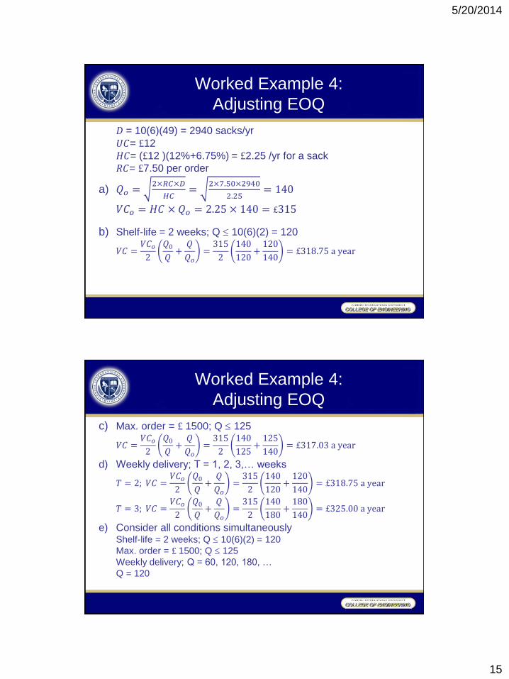
Worked Example 4:

Adjusting EOQ

Jessica Choi works in her bakery for 6 days a week for 49 weeks a

year. Flour is delivered directly with a charge of £7.50 for each

delivery. Jessica uses an average of 10 sacks of whole-grain flour a

day, for which she pays £12 a sack. She has an overdraft at the

bank which costs 12% a year, with spillage, storage, loss and

insurance costing 6.75% a year.

a) What size of delivery should Jessica use and what are the

resulting costs?

b) How much should she order if the flour has a shelf-life of 2

weeks?

c) How much should she order if the bank imposes a maximum

order value of £1,500?

d) If the mill only delivers on Mondays, how much Jessica order

and how often?

5/20/2014

15

Worked Example 4:

Adjusting EOQ

𝐷 = 10(6)(49) = 2940 sacks/yr

𝑈𝐶= £12

𝐻𝐶= (£12 )(12%+6.75%) = £2.25 /yr for a sack

𝑅𝐶= £7.50 per order

a) 𝑄𝑜 =2×𝑅𝐶×𝐷

𝐻𝐶=

2×7.50×2940

2.25= 140

𝑉𝐶𝑜 = 𝐻𝐶 × 𝑄𝑜 = 2.25 × 140 = £315

b) Shelf-life = 2 weeks; Q 10(6)(2) = 120


𝑄0𝑄

+𝑄

𝑄𝑜=315

2

140

120+120

140= £318.75 a year

Worked Example 4:

Adjusting EOQ

c) Max. order = £ 1500; Q 125


𝑄0𝑄

+𝑄

𝑄𝑜=315

2

140

125+125

140= £317.03 a year

d) Weekly delivery; T = 1, 2, 3,… weeks

𝑇 = 2; 𝑉𝐶 =𝑉𝐶𝑜2

𝑄0𝑄+

𝑄

𝑄𝑜=315

2

140

120+120

140= £318.75 a year

𝑇 = 3; 𝑉𝐶 =𝑉𝐶𝑜2

𝑄0𝑄+

𝑄

𝑄𝑜=315

2

140

180+180

140= £325.00 a year

e) Consider all conditions simultaneouslyShelf-life = 2 weeks; Q 10(6)(2) = 120

Max. order = £ 1500; Q 125

Weekly delivery; Q = 60, 120, 180, …

Q = 120

5/20/2014

16

Orders for Discrete Items

• Suppose we calculate the optimal order size as Qo, which is

between the integers Q’−1 and Q’. We should round up the

order size if the variable cost of ordering Q’ units is less

than the variable cost of ordering Q’−1 units.


For 𝑉𝐶(𝑄’) ≤ 𝑉𝐶(𝑄′ − 1),𝑅𝐶 × 𝐷

𝑄′+HC × Q′

2≤𝑅𝐶 × 𝐷

𝑄′ − 1+HC × (Q′ − 1)

2

multiplying both sides by 2×Q’×(Q’−1)

𝐻𝐶(𝑄′)(𝑄′ − 1) ≤ 2(𝑅𝐶)(𝐷)

(𝑄′)(𝑄′ − 1) ≤ 𝑄𝑜2

1. Calculate the EOQ, 𝑄𝑜.

2. Find the integers Q’ and Q’−1 that surround 𝑄𝑜.

3. If Q’× (Q’− 1) is less than or equal to 𝑄𝑜2, order Q’.

4. If Q’× (Q’− 1) is greater than 𝑄𝑜2, order Q’− 1.

5/20/2014

17

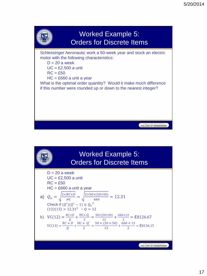
Worked Example 5:


Schlessinger Aeronautic work a 50-week year and stock an electric

motor with the following characteristics:

D = 20 a week

UC = £2,500 a unit

RC = £50

HC = £660 a unit a year

What is the optimal order quantity? Would it make much difference

if this number were rounded up or down to the nearest integer?

Worked Example 5:


D = 20 a week

UC = £2,500 a unit

RC = £50

HC = £660 a unit a year

a) 𝑄𝑜 =2×𝑅𝐶×𝐷

𝐻𝐶=

2×50×(20×50)

660= 12.31

Check if (𝑄′)(𝑄′ − 1) ≤ 𝑄𝑜2

12 13 > 12.312 ∴ 𝑄 = 12

b) VC 12 =𝑅𝐶×𝐷

𝑄+

HC× Q

2=

50×(20×50)

12+

660×12

2= £8126.67

VC 13 =𝑅𝐶 × 𝐷

𝑄+HC × Q′

2=50 × (20 × 50)

13+660 × 13

2= £8136.15

5/20/2014

18

Uncertainty in Demand and Costs:

Error in Demand

• Suppose that actual demand for an item is D, but there is a

proportional error in the forecasts, E. Then the forecast is

𝐷 × (1 + 𝐸) and instead of using the correct EOQ:

𝑄𝑜 =2×𝑅𝐶×𝐷

𝐻𝐶, we used 𝑄 =

2×𝑅𝐶×𝐷×(1+𝐸)

𝐻𝐶

• Since 𝑉𝐶

𝑉𝐶𝑜=

1

2

𝑄0

𝑄+

𝑄

𝑄𝑜

𝑉𝐶

𝑉𝐶𝑜=1

2

1

1 + 𝐸+

1 + 𝐸

1


Error in Demand

0.00%

20.00%

40.00%

60.00%

80.00%

100.00%

120.00%

140.00%

160.00%

-150% -100% -50% 0% 50% 100% 150%

Error in Cost

5/20/2014

19


Error in Costs

• Suppose, for example, that we approximate an actual

reorder cost of RC by RC× (1+ E1), and an actual holding

cost of HC by HC × (1+ E2):

𝑄 =2 × 𝑅𝐶 × (1 + 𝐸1) × 𝐷

𝐻𝐶 × (1 + 𝐸2)

• Since 𝑉𝐶

𝑉𝐶𝑜=

1

2

𝑄0

𝑄+

𝑄

𝑄𝑜

𝑉𝐶

𝑉𝐶𝑜=1

2

1 + 𝐸2

1 + 𝐸1+

1 + 𝐸1

1 + 𝐸2

Reverse Calculation:

Estimating Implied Costs

𝑄0 =2×𝑅𝐶×𝐷

𝐻𝐶, 𝑅𝐶 =

𝑄02×𝐻𝐶

2×𝐷

• If this calculation is repeated, it might be possible to get a

reasonable overall estimate for the reorder cost.

5/20/2014

20

Worked Example 6:

Estimating implied costs

A company has a standing order of 40 units of an item every

month. What can you infer about the costs? If the reorder cost

is actually €160, what is the implied holding cost?

D = 40 a month

RC = €160

𝐻𝐶 =2 × 𝑅𝐶 × 𝐷

𝑄02 =

2 × €160 × 40/𝑚𝑜

402= €8.00/mo

Adjusting the Order Quantity

𝑄 = 𝑘 ×2 × 𝑅𝐶 × 𝐷

𝐻𝐶

𝑄 =2 × 𝑅𝐶 × 𝐷

𝐻𝐶 × 𝑘

• Factor 𝑘 is introduced to make adjustments to the order

quantity.

5/20/2014

21

Adding a Finite Lead Time

Causes of lead time:

• Time for order preparation

• Time to get the order to the right place in suppliers

• Time at the supplier

• Time to get materials delivered from suppliers

• Time to process the delivery

Adding a Finite Lead Time:

Reorder Level

• When demand is constant, there is no benefit in carrying

stock from one cycle to the next, so each order should be

timed to arrive just as existing stock runs out.

• To achieve this, we have to place an order a time LT before

the delivery is needed.

• The easiest way of arranging this is to define a reorder level.

• The EOQ does not depend on lead time and remains

unchanged.

• As both demand and lead time are constant, the amount of

stock needed to cover the lead time is also constant at:

lead time × demand per unit time

5/20/2014

22


Reorder Level

Time

Stock

level

Place

order

Receive

delivery

LT

Reorder

level

Optimal

order sizeQ

𝑅𝑂𝐿 = 𝐷 × 𝐿𝑇

Worked Example 7:

Reorder Level w/Finite Lead Time

Carl Smith uses radiators at the rate of 100 a week, and he

has calculated an EOQ of 250 units. What is his best ordering

policy if lead time is: (a) one week? or (b) two weeks?

D = 100 a week

EOQ = 250

a) LT = 1wk;ROL = 𝐿𝑇 × 𝐷 = 1 × 100 = 100b) LT = 2 wks; ROL = 𝐿𝑇 × 𝐷 = 2 × 100 = 200

5/20/2014

23


Longer Lead Time

• When the lead time is particularly long, there can be several

orders outstanding at any time.

• In particular, when the lead time is between n and n+1 cycle

lengths, giving:

𝑛 × 𝑇 < 𝐿𝑇 < 𝑛 + 1 𝑇• There are n orders outstanding when it is time to place

another. Then we subtract 𝑛 × 𝑄𝑜 from the lead time

demand to get the reorder level:

𝑅𝑂𝐿 = 𝐿𝑇 × 𝐷 − 𝑛 × 𝑄𝑜

Stock Level with Longer Lead Time

Time

Stock

level

Place

order B

Place

order CReceive

delivery B

Receive

delivery C

5/20/2014

24

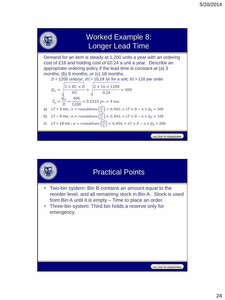
Worked Example 8:

Longer Lead Time

Demand for an item is steady at 1,200 units a year with an ordering

cost of £16 and holding cost of £0.24 a unit a year. Describe an

appropriate ordering policy if the lead time is constant at (a) 3

months; (b) 9 months; or (c) 18 months.𝐷 = 1200 units/yr; 𝐻𝐶= £0.24 /yr for a unit; 𝑅𝐶= £16 per order

𝑄𝑜 =2 × 𝑅𝐶 × 𝐷

𝐻𝐶=

2 × 16 × 1200

0.24= 400


=400

1200= 0.3333 𝑦𝑟. = 4 𝑚𝑜.

a) LT = 3 mo.; 𝑛 = 𝑟𝑜𝑢𝑛𝑑𝑑𝑜𝑤𝑛𝐿𝑇

𝑇𝑜= 0;𝑅𝑂𝐿 = 𝐿𝑇 × 𝐷 − 𝑛 × 𝑄0 = 300

b) LT = 9 mo.; 𝑛 = 𝑟𝑜𝑢𝑛𝑑𝑑𝑜𝑤𝑛𝐿𝑇

𝑇𝑜= 2;𝑅𝑂𝐿 = 𝐿𝑇 × 𝐷 − 𝑛 × 𝑄0 = 100

c) LT = 18 mo.; 𝑛 = 𝑟𝑜𝑢𝑛𝑑𝑑𝑜𝑤𝑛𝐿𝑇

𝑇𝑜= 4;𝑅𝑂𝐿 = 𝐿𝑇 × 𝐷 − 𝑛 × 𝑄0 = 200

Practical Points

• Two-bin system: Bin B contains an amount equal to the

reorder level, and all remaining stock in Bin A. Stock is used

from Bin A until it is empty – Time to place an order.

• Three-bin system: Third bin holds a reserve only for

emergency.

Date post:	16-Mar-2020
Category:	Documents
Upload:	others
View:	2 times
Download:	0 times

Part II Methods for Independent...

Documents