General rights Copyright and moral rights for the publications made accessible in the public portal are retained by the authors and/or other copyright owners and it is a condition of accessing publications that users recognise and abide by the legal requirements associated with these rights.

Users may download and print one copy of any publication from the public portal for the purpose of private study or research.

You may not further distribute the material or use it for any profit-making activity or commercial gain

You may freely distribute the URL identifying the publication in the public portal If you believe that this document breaches copyright please contact us providing details, and we will remove access to the work immediately and investigate your claim.

Downloaded from orbit.dtu.dk on: Jan 24, 2022

Part-load performance of a high temperature Kalina cycle

Modi, Anish; Andreasen, Jesper Graa; Kærn, Martin Ryhl; Haglind, Fredrik

Published in:Energy Conversion and Management

Link to article, DOI:10.1016/j.enconman.2015.08.006

Publication date:2015

Document VersionPeer reviewed version

Link back to DTU Orbit

Citation (APA):Modi, A., Andreasen, J. G., Kærn, M. R., & Haglind, F. (2015). Part-load performance of a high temperatureKalina cycle. Energy Conversion and Management, 105, 453-461.https://doi.org/10.1016/j.enconman.2015.08.006

Part-load performance of a high temperature Kalina cycle

Anish Modi∗, Jesper Graa Andreasen, Martin Ryhl Kærn, Fredrik Haglind

Department of Mechanical Engineering, Technical University of Denmark, Nils Koppels Alle, Building 403,DK-2800 Kgs. Lyngby, Denmark

Abstract

The Kalina cycle has recently seen increased interest as an alternative to the conventionalsteam Rankine cycle. The cycle has been studied for use with both low and high temperatureapplications such as geothermal power plants, ocean thermal energy conversion, waste heatrecovery, gas turbine bottoming cycle and solar power plants. The high temperature cyclelayouts are inherently more complex than the low temperature layouts due to the presenceof a distillation-condensation subsystem, three pressure levels and several heat exchangers.This paper presents a detailed approach to solve the Kalina cycle in part-load operatingconditions for high temperature (a turbine inlet temperature of 500 ◦C) and high pressure(100 bar) applications. A central receiver concentrating solar power plant with direct vapourgeneration is considered as a case study where the part-load conditions are simulated bychanging the solar heat input to the receiver. Compared with the steam Rankine cycle, theKalina cycle has an additional degree of freedom in terms of the ammonia mass fractionwhich can be varied in order to maximize the part-load efficiency of the cycle. The resultsinclude the part-load curves for various turbine inlet ammonia mass fractions, and the fittedequations for these curves.

Keywords: Kalina cycle, part-load, ammonia-water mixture, concentrating solar powerplant

1. Introduction

The Kalina cycle was introduced in 1984 [1] as an alternative to the conventional Rank-ine cycle to be used as a bottoming cycle for combined cycle power plants. It uses a mixtureof ammonia and water as the working fluid, instead of pure water as in the case of a steamRankine cycle. The composition of the ammonia-water mixture could be varied by chang-5

ing the ammonia mass fraction in the mixture, i.e. the ratio of the mass of ammonia inthe ammonia-water mixture to the total mass of the mixture. This change in the compo-sition affects the thermodynamic and the transport properties of the mixture [2]. Since its

∗Corresponding author. Tel.: +45 45251910Email address: anmod@mek.dtu.dk (Anish Modi)

Preprint submitted to Energy Conversion and Management August 22, 2015

Nomenclature

Abbreviations

CSP concentrating solar power

GA genetic algorithm

PPTD pinch point temperature difference,◦C

Symbols

∆h specific enthalpy difference, J kg−1

∆T temperature difference, ◦C

δ tolerance

m mass flow rate, kg s−1

Q heat rate, MW

q heat input relative to the design value

W work or electrical power, MW

η efficiency

A area, m2

cp isobaric specific heat capacity,J kg−1 K−1

Fcu copper loss fraction

ktur turbine constant, kg K0.5 s−1 bar−1

L load relative to the design value

N rotational speed, rpm

p pressure, bar

T temperature, ◦C or K

U overall heat transfer coefficient,W m−2 K−1

X vapour quality

x ammonia mass fraction

Subscripts, including components

c cold fluid

cd condenser

cw condenser cooling water

cy cycle

d design condition

gen generator

i i th control volume

is isentropic

lm logarithmic mean temperature differ-ence, ◦C

m mechanical

mx mixer

net net electrical output from the powercycle

pl relative plant load in part-load condi-tion

pp pinch point temperature difference,◦C

pp,cd minimum pinch point temperaturedifference in the condensers, ◦C

pp,re minimum pinch point temperaturedifference in the recuperators, ◦C

pu pump

re recuperator

rec receiver/boiler

sep separator

spl splitter

thv throttle valve

tur turbine

2

introduction, several uses for the Kalina cycle have been proposed for low temperature ap-plications or low grade heat utilization. Examples include their use in a geothermal power10

plants [3], for waste heat recovery [4–7], for exhaust heat recovery in a gas turbine modularhelium reactor [8], in combined heat and power plants [9,10], coupled with a coal-fired steampower plant for exhaust heat recovery [11], as a part of Brayton-Rankine-Kalina triple cycle[12], and in solar power plants [13,14]. For high temperature applications, the Kalina cycleshave been investigated to be used as gas turbine bottoming cycles [15–18], for industrial15

waste heat recovery, biomass based cogeneration and gas engine waste heat recovery [19],for direct-fired cogeneration applications [20], and in concentrating solar power (CSP) plants[21,22].

There have been discussions regarding the feasibility of using ammonia-water mixtures athigh temperatures due to the nitridation effect resulting in the corrosion of the equipment.20

However, the use of an ammonia-water mixture as the working fluid at high temperaturehas been successfully demonstrated in Canoga Park with turbine inlet conditions of 515 ◦Cand 110 bar [23]. Moreover, a patent by Kalina [24] claims the stability of ammonia-watermixtures along with prevention of nitridation for plant operation preferably up to 1093 ◦Cfor temperature and 689.5 bar for pressure using suitable additives. Water itself prevents25

the ammonia in the mixture from corroding the equipment up to about 400 ◦C, and abovethis temperature, the amount of the additive is far below the threshold for it cause anydamage [25].

None of the previous studies for the Kalina cycles have considered the performance of theKalina cycle in part-load conditions. Moreover, the layout for the high temperature Kalina30

cycles is inherently more complex than those used for the low temperature applications. Thisis primarily because of the presence of a distillation-condensation subsystem, at least threepressure levels and several heat exchangers. In applications such as solar power plants wherethe heat input fluctuates throughout the day, and over the year, it is essential to includethe part-load performance of the power cycle to assess the plant performance in a thorough35

manner. Similarly, it is also necessary to evaluate the part-load performance of the powercycle in other cases such as waste heat recovery from diesel engines or other fluctuatingsources of energy input. The Kalina cycles have an additional degree of freedom in termsof the ammonia mass fraction, as compared with using pure working fluids, which makesit possible to obtain better part-load performance characteristics by changing the ammonia40

mass fraction to suit the part-load conditions. To the authors’ knowledge, only Kalinaand Leibowitz [26] and Smith et al. [27] presented performance curves for the part-loadconditions using a Kalina cycle. Kalina and Leibowitz [26] mentioned that the second lawefficiency of the Kalina bottoming cycle for a gas turbine changes by about 3.2 percentagepoints when the cycle load reduces by 25 %. The paper did not present any details about45

the assumptions or the methodology used for calculating the part-load performance of theKalina cycle. Moreover, the part-load performance until only 75 % plant load was presented.

Smith et al. [27] presented the part-load performance curves for a simple gas turbinecycle, a Rankine combined cycle, and a Kalina combined cycle. The Kalina combined cycleshowed the best performance. The operational advantages of the Kalina cycle as compared50

with the Rankine cycle were also presented. This paper also did not provide the part-load

3

characteristics of only the Kalina cycle, or any methodology for evaluating the part-loadperformance characteristics. From the Kalina combined cycle part-load curve, the part-loadperformance of only the Kalina cycle cannot be estimated without knowing the combinedcycle operation and control strategy, which was also not presented in the paper. A recent55

patent by Mlcak and Mirolli [28] suggests varying the ammonia mass fraction in order toimprove the system performance of the Kalina cycle with varying ambient conditions. Thepatent however discusses a relatively simpler low temperature application layout to be usedwith geothermal hot water or industrial waste heat sources.

The objective of this paper is to present the detailed methodology of solving a Kalina60

cycle at part-load conditions for high temperature applications. As a case, a central receiverCSP plant with direct vapour generation is considered. The part-load conditions were sim-ulated by changing the solar heat input to the receiver, and the cycle was solved in partload by varying the separator inlet ammonia mass fraction and adjusting the pump outletpressures. In the paper, Section 2 presents the design point optimization and the part-load65

modelling approaches along with the assumptions; Section 3 presents the results from thepart-load modelling; Section 4 discusses the results; and Section 5 concludes the paper.

2. Methods

The Kalina cycle layout investigated in this paper, named KC12 [22], is shown in Fig. 1.The cycle components in the layout are shown in abbreviated forms where REC is the70

receiver/boiler, TUR is the turbine, GEN is the generator, SEP is the vapour-liquid sepa-rator, RE∗ is the recuperator, PU∗ is the pump, CD∗ is the condenser, MX∗ is the mixer(where ‘∗’ denotes the respective component number), SPL is the splitter and THV is thethrottling valve.

In the cycle, the superheated ammonia-water mixture (stream 1), i.e. the working solu-75

tion, expands in the turbine and is subsequently mixed in the mixer MX1 with the ammonialean liquid from the separator SEP to lower the ammonia mass fraction in the condenserCD1. The fluid after the mixer MX1 is called the basic solution. The ammonia rich vapourfrom the separator SEP is later mixed in the mixer MX2 with a part of the basic solutionfrom the splitter SPL to again form the working solution. This working solution then goes80

through the condenser CD2 and the pump PU2. The external heat input to the workingfluid is provided in the boiler. In the case considered in this study, the boiler is the solarreceiver REC.

All the simulations were performed using MATLAB R2015a [29]. The thermodynamicproperties for the ammonia-water mixtures were calculated using the REFPROP 9.1 inter-85

face for MATLAB [30]. The default property calculation method for the ammonia-watermixtures in REFPROP is using the Tillner-Roth and Friend formulation [31]. However,this formulation in REFPROP is highly unstable and fails to converge on several occasions,especially in the two-phase regions, near the critical point and at higher ammonia massfractions. Therefore, an alternative formulation called ’Ammonia (Lemmon)’ [32] was used.90

It was found to be more stable and with fewer convergence failures, without significantlycompromising on the accuracy of the calculations [22].

4

Figure 1: Kalina cycle KC12.

2.1. Design optimization

In order to model the Kalina cycle in part-load conditions, it was first necessary toobtain the cycle performance characteristics and the thermodynamic states at the design95

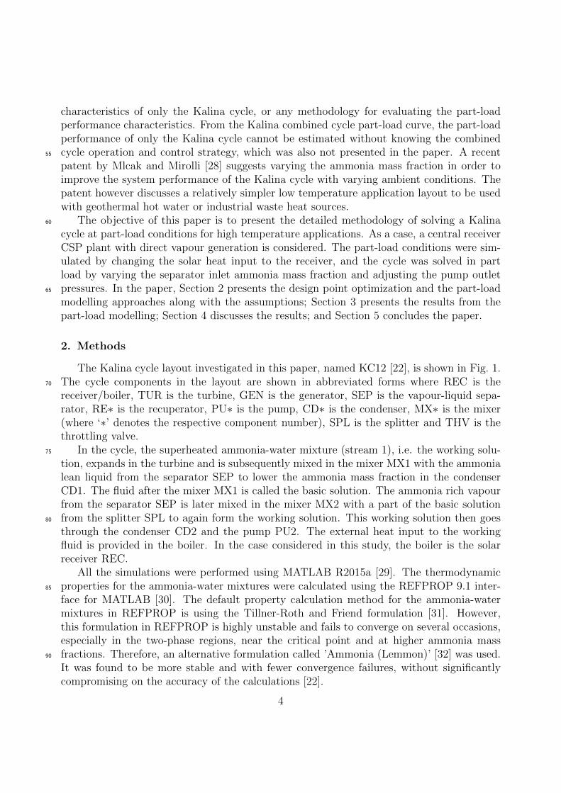
point of operation. A detailed methodology to solve and optimize the Kalina cycle at designpoint using a genetic algorithm (GA) was presented by Modi and Haglind [22]. For theKC12 layout (Fig. 1), the algorithm to optimize the cycle and obtain the design conditionparameters is shown in Fig. 2. The cycle was thermodynamically optimized by maximizingthe cycle efficiency for a given net electrical power output. The turbine outlet pressure,100

the separator inlet temperature and the separator inlet ammonia mass fraction were thedecision variables for the optimization. The turbine inlet ammonia mass fraction was variedfor parametric analysis in order to analyse the cycle behaviour for a range of values. Thefollowing assumptions were made for the cycle design optimization [18,22]:

a. The cycle was modelled in steady state.105

b. The turbine inlet temperature and pressure were fixed at 500 ◦C and 100 bar. The

5

isentropic efficiencies of the turbine and the pumps were 85 % and 70 % respectively.The turbine mechanical efficiency and the generator efficiency were both 98 %.

c. The plant was designed for a net electrical power output of 20 MW. The minimum allowedvapour quality at the turbine outlet was 90 %. The condenser cooling water inlet and110

outlet temperatures were fixed at 20 ◦C and 30 ◦C.

d. The recuperators and the condensers had a minimum pinch point temperature difference(PPTD) of 8 ◦C and 4 ◦C respectively.

e. Pressure drops and heat losses were neglected.

f. The minimum separator inlet vapour quality was fixed at 5 %.115

Figure 2: Solution algorithm for every iteration of the Kalina cycle KC12 for design calculation using GA.

6

In general, the following steps were used to solve the Kalina cycle for each iteration of theoptimization process. The turbine TUR was solved first to obtain the state at the turbineoutlet. Assuming a condenser pressure for the condenser CD2, the mass flow rates were thenobtained using a simplified configuration as presented by Marston [15]. With respect to themass flow rates at different points in the cycle, the entire cycle can be represented by the120

simplified layout as shown in Fig. 3.

Figure 3: Simplified configuration of the Kalina cycle KC12 with respect to different mass flow rates in thecycle.

The mass balance equations for the ammonia-water mixture and ammonia in the mixture,and the ammonia mass fraction balance equations are:

m5 = m1 + m12 (1)

m5 · x5 = m1 · x1 + m12 · x12 (2)

m1 = m8 + m11 (3)

m1 · x1 = m8 · x8 + m11 · x11 (4)

m10 = m11 + m12 (5)

m10 · x10 = m11 · x11 + m12 · x12 (6)

m11 = m10 ·X10 (7)

x5 = x10 (8)

x8 = x10 (9)

where m is the mass flow rate, x is the ammonia mass fraction and X is the vapour quality.The mass balances are over the mixer MX1 (Eqs. 1 and 2), the mixer MX2 (Eqs. 3 and

4) and the separator SEP (Eqs. 5 and 6). The ammonia mass fraction balances are over thesplitter SPL (Eqs. 8 and 9). Since the separator SEP is simply a vapour-liquid separator,Eq. 7 only relates the mass flow rate of stream 11 to the mass flow rate and the vapourquality of the stream 10. On rearranging the above equations, the following relations are

7

obtained:

m10

m1

=x1 − x10

X10 · (x11 − x10)(10)

m8

m1

=x11 − x1x11 − x10

(11)

These relations were then used to calculate the different mass flow rates after assumingm1 to be 1 kg s−1 as an initial guess value, and calculating the values of the ammoniamass fractions for the two outlet streams of the separator (x11 and x12) with REFPROP125

using the state at the separator inlet as input. This was done repeatedly until the PPTDin the condenser CD2 became greater than or equal to the minimum PPTD value for thecondensers.

Once the mass flow rates at different points in the cycle were known, and it was madesure that the inlet stream to the separator SEP is in two-phase flow, then the pumps, the130

mixers, the recuperators and the condensers were solved while satisfying all the designconstraints such as minimum PPTD, minimum vapour quality at the turbine outlet, etc.and using the following equations:

TUR: Wtur = m1 · (h1 − h2) (12)135

GEN: Wgen = Wtur · ηtur,m · ηgen (13)RE1: m2 · (h2 − h3) = m16 · (h17 − h16) (14)RE2: m3 · (h3 − h4) = m9 · (h10 − h9) (15)CD1: m5 · (h5 − h6) = mcw,cd1 · cp,cw · (Tcw,out − Tcw,in) (16)CD2: m14 · (h14 − h15) = mcw,cd2 · cp,cw · (Tcw,out − Tcw,in) (17)140

PU1: Wpu1 = m6 · (h7 − h6) (18)PU2: Wpu2 = m15 · (h16 − h15) (19)SEP: m10 · h10 = m11 · h11 + m12 · h12 (20)MX1: m5 · h5 = m4 · h4 + m13 · h13 (21)MX2: m14 · h14 = m8 · h8 + m11 · h11 (22)145

SPL: h8 = h7 (23)SPL: h9 = h7 (24)THV: h12 = h13 (25)

where Wtur, Wpu and Wgen are respectively the turbine work output, the required150

pump work and the generator electrical power output, m is the mass flow rate, h is thespecific enthalpy, cp is the isobaric specific heat capacity, and T is the temperature. Thesubscript ‘cw’ denotes the condenser cooling water.

The cycle efficiencies from the different combinations of the decision variables were com-pared, and the solution with the highest cycle efficiency was stored as the optimal solution155

for the given input of the turbine inlet ammonia mass fraction. The same procedure wasthen repeated for different values of the turbine inlet ammonia mass fractions. All the heatexchangers, including the condensers, were discretized into 50 control volumes and solved sothat the position of the PPTD could be calculated with sufficient accuracy. The UA values,

8

i.e. the ratio of the heat transferred in any control volume to the logarithmic mean tem-160

perature difference over the control volume, for the different heat exchangers were obtainedfrom:

(UA)i,d =Qi,d

∆Tlm,i,d

(26)

where U , A, Q and ∆Tlm are respectively the overall heat transfer coefficient, heat transferarea, the heat transfer rate and the logarithmic mean temperature difference for the ith

control volume at design point of operation.165

2.2. Validation

In order to ensure the mathematical accuracy of the solution algorithm for the Kalina cy-cle, several check parameters related to the mixture mass balances, ammonia mass balancesand energy balances over the different cycle components were included in the process. It wasensured that all the balances were satisfied with a residual below or equal to 0.001 %. The170

same was considered for the part-load model. In case there was an error in the calculationof the thermodynamic properties by REFPROP, or the balances were not satisfied withinthe specified tolerance, the solution was rejected.

To the authors’ knowledge, there is no publication mentioning the operating states ofa high temperature Kalina cycle that were either obtained experimentally, or from the175

measurements taken from a commercial plant. It was therefore only possible to validatethe Kalina cycle models with the results from previously published modelling results. OnlyMarston [15] provides all the modelling assumptions and results in order to make a propervalidation. The layout investigated by Marston [15] is what was referred to as KC234 in Modiand Haglind [22]. In order to validate the overall solution methodology, this layout was used.180

For different combinations of the turbine inlet ammonia mass fraction and the separator inlettemperature taken from Marston [15], it was found that the maximum deviation of the cycleefficiency values calculated from the current algorithm from those presented in Marston [15]was 2.21 %, with the average deviation being 1.01 %. This is using the same modellingassumptions as mentioned in Marston [15], but with the Kalina cycle solution methodology185

as used in Modi and Haglind [22], and in the current study. With these low deviations,the current solution algorithm was considered validated. The reason for selecting the KC12layout to investigate the part-load performance of the Kalina cycle was because this layoutwas overall found to be more efficient than KC234 [22], while being simpler with fewernumber of recuperators.190

2.3. Part-load modelling

Once the thermodynamic states, the mass flow rates and the UA values were obtainedfrom the cycle design optimization, the part-load calculations were performed. The heatinput to the receiver REC was gradually decreased and the part-load relative efficiencycurves for different plant loads and turbine inlet ammonia mass fractions were prepared.195

A solution algorithm similar to the validated design optimization algorithm was used forthe part-load performance calculations, but with different decision variables and additional

9

assumptions required for the part-load calculations. The following assumptions were madefor the Kalina cycle steady-state part-load calculations. The turbine inlet temperature wasmaintained at the design value of 500 ◦C to have the highest temperature at the turbine200

inlet for better efficiency. The turbine inlet ammonia mass fraction was maintained at itsrespective design point value in order to avoid fluctuations in the turbine output as suggestedin Amano et al. [33]. The condenser cooling water inlet temperature was assumed to be thesame as its design value, as has been done in Lippke [34]. In order to satisfy the condensingload, the condenser cooling water mass flow rate would then adjusted by regulating the205

cooling water pump. The minimum separator inlet vapour quality was fixed at 2 %, avalue smaller than the design value, but enough to ensure that there will be a two-phaseflow at the separator inlet. The separator inlet ammonia mass fraction was allowed to varywithin ±1 % of the design value to enable using the power law for heat exchanger off-designcalculations. The condensers’ working fluid outlet temperature was at least 2 ◦C higher than210

the cooling water inlet temperature. The tolerance δ in Fig. 4 was set to 0.1 K. A moreelaborate discussion regarding the part-load modelling assumptions is provided in Section 4.

The turbine was modelled in part load using the Stodola’s ellipse law (Eq. 27) to calculatethe turbine constant [35], and the off-design isentropic efficiency (Eq. 28) as described inRay [36]:215

ktur =m1 ·√T1√

p21 − p22(27)

ηtur,is = ηtur,is,d − 2 ·

[N

Nd

·√

∆his,d∆his

− 1

]2(28)

where ktur is the turbine constant, ηtur,is and ηtur,is,d are the turbine isentropic efficiencies atpart-load and design conditions, N and Nd are the turbine rotational speeds at part-loadand design conditions, and ∆his and ∆his,d are the isentropic specific enthalpy differencesat part-load and design conditions. The turbine speed in a power plant remains constant in220

order to maintain the generated electricity frequency, and therefore the ratio of the speedsin Eq. 28 is taken as unity [36]. The mechanical efficiency of the turbine was assumed thesame as its design value.

The off-design isentropic efficiency of the pumps was obtained using [34]:

ηpu,is = ηpu,is,d ·

[2 · m

md

−(m

md

)2]

(29)

where ηpu,is and ηpu,is,d are pump efficiencies at part-load and design conditions, and m and225

md are the mass flow rates through the pump at part-load and design conditions.The off-design generator efficiency was obtained using [37]:

ηgen =ηgen,d · Lgen

ηgen,d · Lgen + (1− ηgen,d) ·[(1− Fcu) + Fcu · L2

gen

] (30)

10

where Fcu is the copper loss fraction (assumed 0.43 [37]), ηgen and ηgen,d are the generatorefficiencies at part-load and design conditions, and Lgen is the generator load relative to thedesign value.230

The heat exchangers were discretized once again in the part-load conditions to calculatethe temperature profiles. As a first approximation, the UA values in part load for eachcontrol volume was obtained using the power law with the cold side mass flow rate [38]:

(UA)i = (UA)i,d ·(mc

mc,d

)0.8

(31)

where (UA)i and (UA)i,d are the UA values at part-load and design conditions for the ith

control volume in W K−1, and mc and mc,d are the mass flow rates of the cold fluid at235

part-load and design conditions.For the part-load operation, the following control strategy was used. The turbine inlet

pressure was varied in a sliding pressure operation to maintain the turbine inlet temperatureat the design value. In order to obtain the highest part-load performance from the cycle, theseparator inlet ammonia mass fraction was varied. In practice, it is easier to measure the240

temperatures and pressures in the cycle than the ammonia mass fraction, especially whenthe mixture is in two-phase flow. Since the pressure at the pump PU1 outlet is governedby the condenser CD2, the splitter SPL split fraction (i.e. the ratio of the mass flow rateof stream 9 to that of stream 7 in Fig. 1) needs to be varied to obtain the required optimalseparator inlet ammonia mass fraction. This split fraction can be varied by changing the245

splitter SPL valve position, and this position in turn determines the separator inlet ammoniamass fraction. For a given value of the pump PU1 outlet pressure (which is also the separatorinlet pressure), there will be only one combination of the temperature and the ammonia massfraction at the separator inlet which results in the highest part-load performance. Thus, theseparator SEP inlet temperature can be monitored in order to specify the optimal splitter250

valve position, and thus the optimal split fraction.The Kalina cycle was solved in part load using Eqs. 1-11 and 27-31 in the algorithm

shown in Fig. 4 where the numbers in the subscript and the component names correspondto the cycle layout in Fig. 1. In practice, it is the pumps and the splitter which will beregulated, however for modelling purposes, it is better to provide the ammonia mass fraction255

as the varying parameter rather than the split fraction as it speeds up the computationsignificantly [22]. This is because the ammonia mass fraction is always required as an inputto calculate the thermophysical properties for the mixture, and therefore providing it as aninput considerably reduces the number of required iterations.

11

Figure 4: Part-load solution algorithm for the Kalina cycle KC12.

3. Results260

Fig. 5 shows the optimal cycle efficiency values for the different turbine inlet ammoniamass fractions. The trend of the variation in the cycle efficiency with the turbine inletammonia mass fraction was explained in detail for the KC12 layout by Modi and Haglind [21].In short, the rate of exergy destruction in the two condensers CD1 and CD2, the recuperatorRE1 and the turbine TUR shows a decreasing trend; whereas the rate of exergy destruction265

in the recuperator RE2 first increases and then decreases. Similarly, the rate of exergydestruction in the throttle valve THV and the mixers MX1 and MX2 becomes negligibleat higher values of turbine inlet ammonia mass fraction due to a better match betweenthe temperatures of the mixing streams. The combination of these trends causes the cycleefficiency to first drop and then increase after reaching a minimum value.270

12

Figure 5: Optimal cycle efficiency values for different turbine inlet ammonia mass fractions.

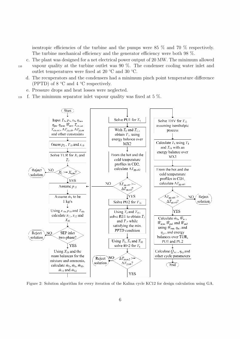
The exemplary state points for the optimal design point for the Kalina cycle KC12 ata turbine inlet ammonia mass fraction of 0.6 are shown in Table 1. The variation in thedecision variable values for the optimal part-load performance for the same case is shown inTable 2.

Table 1: Operation state points for the optimal design at a turbine inlet ammonia mass fraction of 0.6.

Stream T (◦C) p (bar) m (kg/s) x h (kJ/kg)1 500.0 100.00 26.06 0.6000 3032.72 117.5 1.89 26.06 0.6000 2214.23 88.0 1.89 26.06 0.6000 1856.74 33.8 1.89 26.06 0.6000 679.15 45.4 1.89 89.07 0.4037 340.16 24.2 1.89 89.07 0.4037 -21.47 24.2 4.92 89.07 0.4037 -20.98 24.2 4.92 16.86 0.4037 -20.99 24.2 4.92 72.22 0.4037 -20.910 70.0 4.92 72.22 0.4037 404.111 70.0 4.92 9.20 0.9597 1802.712 70.0 4.92 63.01 0.3225 199.913 49.2 1.89 63.01 0.3225 199.914 49.4 4.92 26.06 0.6000 623.115 24.0 4.92 26.06 0.6000 70.816 25.9 100.00 26.06 0.6000 87.917 96.1 100.00 26.06 0.6000 445.3

13

Table 2: Decision variable values at the optimal part-load solutions for a turbine inlet ammonia mass fractionof 0.6.

Lpl p1 (bar) T10 (◦C) x101.000 100 70.00 0.40370.899 89.64 66.60 0.40290.791 79.95 67.60 0.40210.683 70.30 68.50 0.40200.575 60.70 69.65 0.40280.468 50.96 66.60 0.4005

The part-load performance curves for different turbine inlet ammonia mass fractions are275

shown in Fig. 6, while the variation in the relative plant load with the relative heat input isshown in Fig. 7. In the figures, the relative plant load is the ratio of the cycle net electricalpower output in part load to that at the design point, the relative cycle efficiency is theratio of the cycle efficiency in part load to that at the design point, and the relative heatinput is the ratio of the heat input to the receiver REC in part load to that at the design280

point.

Figure 6: Part-load relative cycle efficiency for different design turbine inlet ammonia mass fractions andplant loads.

The equations representing the four part-load curves were generated using the CurveFitting Toolbox of MATLAB. These are shown in Table 3. The equations were fitted withpolynomial fitting option and a robust least-squares fitting method (Least Absolute Resid-uals or LAR), both standard options in the toolbox. The fitted equations for the relative285

heat input as a function of the plant load are shown in Table 4. In the equations, Lpl is therelative plant load and qpl is the relative heat input. All the equations have a coefficient ofdetermination (R2) greater than 0.997.

14

Figure 7: Part-load relative plant load for different design turbine inlet ammonia mass fractions and relativeheat inputs.

Table 3: Part-load relative cycle efficiency as a function of the relative plant load.

x1 Part-load relative cycle efficiency0.5 −0.1641 · L2

pl + 0.3732 · Lpl + 0.79090.6 −0.08693 · L3

pl − 0.01653 · L2pl + 0.291 · Lpl + 0.8125

0.7 −0.2757 · L2pl + 0.5554 · Lpl + 0.7203

0.8 −0.3175 · L2pl + 0.6542 · Lpl + 0.6633

Table 4: Part-load relative plant load as a function of the relative heat input.

x1 Part-load relative plant load0.5 −0.3601 · q3pl + 0.8127 · q2pl + 0.4823 · qpl + 0.065130.6 −0.3333 · q3pl + 0.6960 · q2pl + 0.6031 · qpl + 0.034190.7 −0.3524 · q3pl + 0.7079 · q2pl + 0.6379 · qpl + 0.0066260.8 −0.3961 · q3pl + 0.8040 · q2pl + 0.5953 · qpl − 0.00322

4. Discussion

A Kalina cycle layout suitable for high temperature applications is inherently complex290

in nature including multiple recuperators, condensers, pumps, and an internal separatorloop. Solving such a cycle in both design and part-load conditions presents a significantchallenge. With regards to the part-load operation, Kalina and Leibowitz [26] presented acurve for the second law efficiency for a Kalina cycle operating as a gas turbine bottomingcycle. The paper suggests that for the part-load operation, the mass flow rate through the295

Kalina cycle turbine could be kept constant while varying the turbine inlet ammonia massfraction so as to vary the enthalpy drop across the turbine. In the current study, the turbineinlet ammonia mass fraction was however maintained at its design value during part-load

15

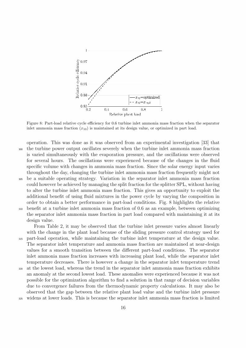
Figure 8: Part-load relative cycle efficiency for 0.6 turbine inlet ammonia mass fraction when the separatorinlet ammonia mass fraction (x10) is maintained at its design value, or optimized in part load.

operation. This was done as it was observed from an experimental investigation [33] thatthe turbine power output oscillates severely when the turbine inlet ammonia mass fraction300

is varied simultaneously with the evaporation pressure, and the oscillations were observedfor several hours. The oscillations were experienced because of the changes in the fluidspecific volume with changes in ammonia mass fraction. Since the solar energy input variesthroughout the day, changing the turbine inlet ammonia mass fraction frequently might notbe a suitable operating strategy. Variation in the separator inlet ammonia mass fraction305

could however be achieved by managing the split fraction for the splitter SPL, without havingto alter the turbine inlet ammonia mass fraction. This gives an opportunity to exploit theadditional benefit of using fluid mixtures in the power cycle by varying the composition inorder to obtain a better performance in part-load conditions. Fig. 8 highlights the relativebenefit at a turbine inlet ammonia mass fraction of 0.6 as an example, between optimizing310

the separator inlet ammonia mass fraction in part load compared with maintaining it at itsdesign value.

From Table 2, it may be observed that the turbine inlet pressure varies almost linearlywith the change in the plant load because of the sliding pressure control strategy used forpart-load operation, while maintaining the turbine inlet temperature at the design value.315

The separator inlet temperature and ammonia mass fraction are maintained at near-designvalues for a smooth transition between the different part-load conditions. The separatorinlet ammonia mass fraction increases with increasing plant load, while the separator inlettemperature decreases. There is however a change in the separator inlet temperature trendat the lowest load, whereas the trend in the separator inlet ammonia mass fraction exhibits320

an anomaly at the second lowest load. These anomalies were experienced because it was notpossible for the optimization algorithm to find a solution in that range of decision variablesdue to convergence failures from the thermodynamic property calculations. It may also beobserved that the gap between the relative plant load value and the turbine inlet pressurewidens at lower loads. This is because the separator inlet ammonia mass fraction is limited325

16

to ±1 % variation from the design value, and it restricts the turbine inlet pressure fromgoing below a certain value to avoid pinch violation in the recuperator RE1.

Fig. 6 shows the trend of the part-load performance of the Kalina cycle with relativeplant load. The curves show a decreasing performance with the decreasing plant load. Itmay be observed that the part-load performance at high plant loads (above 90 %) is almost330

the same for all the turbine inlet ammonia mass fractions because of operating close tothe design point. However, the trends of the performance curves differ when going towardslower plant loads. The part-load performance of the cycle with higher values of turbineinlet ammonia mass fraction (0.7 and above) decreases more rapidly with decreasing plantload as compared with the lower values of the turbine inlet ammonia mass fraction. This is335

because of the significant differences in the basic solution ammonia mass fraction (stream 5in Fig. 1), and therefore the condensing pressures. For example, the condenser CD1 pressure(also the turbine outlet pressure) at 50 % relative heat input for 0.6 and 0.8 turbine inletammonia mass fractions is respectively 1.70 and 5.56 bar, whereas the turbine inlet pressuresfor the two cases are almost the same at 50.96 and 52.85 bar respectively. This results in340

less expansion in the turbine at low plant loads for 0.8 turbine inlet ammonia mass fractionresulting in a lower part-load efficiency for the same relative heat input. The higher theworking solution ammonia mass fraction is, the higher the basic solution ammonia massfraction will be for the Kalina cycle to operate. The higher the basic solution ammoniamass fraction is, the higher the condensing pressure will be. In fact this is the reason to345

have the distillation-condensation subsystem in the first place - to reduce the ammonia massfraction in the condenser CD1 so that the working solution in the turbine can be expandedto lower pressures. Therefore, even though a higher working solution ammonia mass fractionmight result in a higher design point efficiency because of more effective recuperation andcondensation [22], it might also result in lower part-load performance at low plant loads350

because of a larger relative reduction in the turbine inlet pressure than the correspondingturbine outlet pressure relative reduction.

5. Conclusion

The Kalina cycle was modelled and its part-load performance was investigated. Forthe part-load modelling, the temperature and the ammonia mass fraction at the turbine355

inlet were maintained at the design values. The separator inlet ammonia mass fraction wasvaried in order to obtain the highest efficiency at different loads. In practice, it would be thepumps and the splitter which would be regulated in order to obtain the optimal part-loadoperating conditions. However, for numerical analysis, it is better to provide the ammoniamass fraction as an input to speed up the computation. The part-load performance curves360

and their fitted equations are presented for various plant loads and turbine inlet ammoniamass fractions. The part-load performance at higher plant loads is almost the same forthe different ammonia mass fractions, whereas at lower plant loads, the part-load efficiencydecreases rapidly for higher values of the turbine inlet ammonia mass fractions.

17

References365

[1] A.I. Kalina. Combined-cycle system with novel bottoming cycle. Journal of Engineering for GasTurbines and Power, 106:737–742, 1984.

[2] M.R. Kærn, A. Modi, J.K. Jensen, and F. Haglind. An assessment of transport property estimationmethods for ammonia-water mixtures and their influence on heat exchanger size. International Journalof Thermophysics, 2015. Available online, doi:10.1007/s10765-015-1857-8.370

[3] A. Coskun, A. Bolatturk, and M. Kanoglu. Thermodynamic and economic analysis and optimizationof power cycles for a medium temperature geothermal resource. Energy Conversion and Management,78:39–49, February 2014.

[4] P. Bombarda, C.M. Invernizzi, and C. Pietra. Heat recovery from diesel engines: A thermodynamiccomparison between Kalina and ORC cycles. Applied Thermal Engineering, 30(2-3):212–219, 2010.375

[5] H. Junye, C. Yaping, and W. Jiafeng. Thermal performance of a modified ammonia-water power cyclefor reclaiming mid/low-grade waste heat. Energy Conversion and Management, 85:453–459, 2014.

[6] C. Yue, D. Han, W. Pu, and W. He. Comparative analysis of a bottoming transcritical ORC and aKalina cycle for engine exhaust heat recovery. Energy Conversion and Management, 89:764–774, 2015.

[7] P. Zhao, J. Wang, and Y. Dai. Thermodynamic analysis of an integrated energy system based on380

compressed air energy storage (CAES) system and Kalina cycle. Energy Conversion and Management,98:161–172, 2015.

[8] V. Zare, S.M.S. Mahmoudi, and M. Yari. On the exergoeconomic assessment of employing Kalina cyclefor GT-MHR waste heat utilization. Energy Conversion and Management, 90:364–374, 2015.

[9] S. Ogriseck. Integration of Kalina cycle in a combined heat and power plant, a case study. Applied385

Thermal Engineering, 29(14-15):2843–2848, 2009.[10] Z. Zhang, Z. Guo, Y. Chen, J. Wu, and J. Hua. Power generation and heating performances of integrated

system of ammonia-water Kalina-Rankine cycle. Energy Conversion and Management, 92:517–522,2015.

[11] O.K. Singh and S.C. Kaushik. Energy and exergy analysis and optimization of Kalina cycle coupled390

with a coal fired steam power plant. Applied Thermal Engineering, 51(1-2):787–800, 2013.[12] O.K. Singh and S.C. Kaushik. Thermoeconomic evaluation and optimization of a Brayton-Rankine-

Kalina combined triple power cycle. Energy Conversion and Management, 71:32–42, 2013.[13] J. Wang, Z. Yan, E. Zhou, and Y. Dai. Parametric analysis and optimization of a Kalina cycle driven

by solar energy. Applied Thermal Engineering, 50(1):408–415, 2013.395

[14] F. Sun, W. Zhou, Y. Ikegami, K. Nakagami, and X. Su. Energy-exergy analysis and optimization ofthe solar-boosted Kalina cycle system 11 (KCS-11). Renewable Energy, 66:268–279, 2014.

[15] C.H. Marston. Parametric analysis of the Kalina cycle. Journal of Engineering for Gas Turbines andPower, 112:107–116, 1990.

[16] C.H. Marston and M. Hyre. Gas turbine bottoming cycles: Triple-pressure steam versus Kalina. Journal400

of Engineering for Gas Turbines and Power, 117(January):10–15, 1995.[17] M.B. Ibrahim and R.M. Kovach. A Kalina cycle application for power generation. Energy, 18(9):961–

969, 1993.[18] P.K. Nag and A.V.S.S.K.S. Gupta. Exergy analysis of the Kalina cycle. Applied Thermal Engineering,

18(6):427–439, 1998.405

[19] E. Thorin. Power cycles with ammonia-water mixtures as working fluid. Phd thesis, KTH RoyalInstitute of Technology, Stockholm, 2000.

[20] C. Dejfors, E. Thorin, and G. Svedberg. Ammonia-water power cycles for direct-fired cogenerationapplications. Energy Conversion and Management, 39(16-18):1675–1681, 1998.

[21] A. Modi and F. Haglind. Performance analysis of a Kalina cycle for a central receiver solar thermal410

power plant with direct steam generation. Applied Thermal Engineering, 65(1-2):201–208, 2014.[22] A. Modi and F. Haglind. Thermodynamic optimisation and analysis of four Kalina cycle layouts for

high temperature applications. Applied Thermal Engineering, 76:196–205, 2015.[23] M. D. Mirolli. Kalina cycle power systems in waste heat recovery applications, 2012.

18

[24] A.I. Kalina. Method of preventing nitridation or carburization of metals. United States Patent 6482272415

B2, 2002.[25] Kalex LLC. Kalina cycle power systems for solar-thermal applications, 2015.[26] A.I. Kalina and H.M. Leibowitz. Off-design perfomance, equipment considerations, and material selec-

tion for a Kalina system 6 bottoming cycle. In ASME COGEN-TURBO, 3rd International Symposiumon Turbomachinery, Combined-Cycle Technologies and Cogeneration, volume 4, pages 347–355, Nice,420

France, 1989. ASME.[27] R.W. Smith, J. Ranasinghe, D. Stats, and S. Dykas. Kalina combined cycle performance and operability.

In PWR Joint Power Generation Conference, volume 30, pages 701–727. ASME, 1996.[28] H.A. Mlcak and M.D. Mirolli. Systems and methods for increasing the efficiency of a Kalina cycle.

United States Patent US8744636B2, 2014.425

[29] MathWorks. MATLAB. www.mathworks.se/products/matlab, 2015.[30] National Institute for Standards and Technology. REFPROP MATLAB Interface.

www.boulder.nist.gov/div838/theory/refprop/Frequently asked questions.htm#MatLabApplications,2015.

[31] R. Tillner-Roth and D.G. Friend. A Helmholtz free energy formulation of the thermodynamic properties430

of the mixture {water+ammonia}. Journal of Physical and Chemical Reference Data, 27(1):63–96, 1998.[32] E. Lemmon. Private communication, 2013.[33] Y. Amano, K. Kawanishi, and T. Hashizume. Experimental investigations of oscillatory fluctuation

in an ammonia-water mixture turbine system. In Proceedings of IMECE International MechanicalEngineering Congress and Exposition, volume 45, pages 391–398, Ontario, Florida, USA, 2005. ASME.435

[34] F. Lippke. Simulation of the part-load behavior of a 30 MWe SEGS plant. Technical report, SandiaNational Laboratories SAND95-1293, 1995.

[35] D.H. Cooke. Modeling of off-design multistage turbine pressures by Stodola’s ellipse. In Energy Incor-porated PEPSE User’s Group Meeting, pages 205–234, Richmond, Virginia, USA, 1983. Bechtel PowerCorporation.440

[36] A. Ray. Dynamic modelling of power plant turbines for controller design. Applied MathematicalModelling, 4(2):109–112, 1980.

[37] F. Haglind and B. Elmegaard. Methodologies for predicting the part-load performance of aero-derivativegas turbines. Energy, 34(10):1484–1492, 2009.

[38] P. Schwarzbozl. A TRNSYS model library for solar thermal electric components (STEC). Technical445

report, Deutsches Zentrum fur Luft und Raumfahrt e.V. (DLR), Cologne, Germany, 2006.

19