PART VI

LQR/LQG OPTIMAL CONTROL

LECTURE 20

Linear Quadratic Regulation (LQR)

CONTENTS

This lecture introduces the most general form of the linear quadratic regulation problem and solves it using an appropriate feedback invariant.

1. Deterministic Linear Quadratic Regulation (LQR)

2. Optimal Regulation

3. Feedback Invariants

4. Feedback Invariants in Optimal Control

5. Optimal State Feedback

6. LQR in MATLAB®

7. Additional Notes

8. Exercises

20.1 DETERMINISTIC LINEAR QUADRATIC REGULATION (LQRl

Attention! Note the negative feedback and the absence of a reference signal in Figure 20.1.

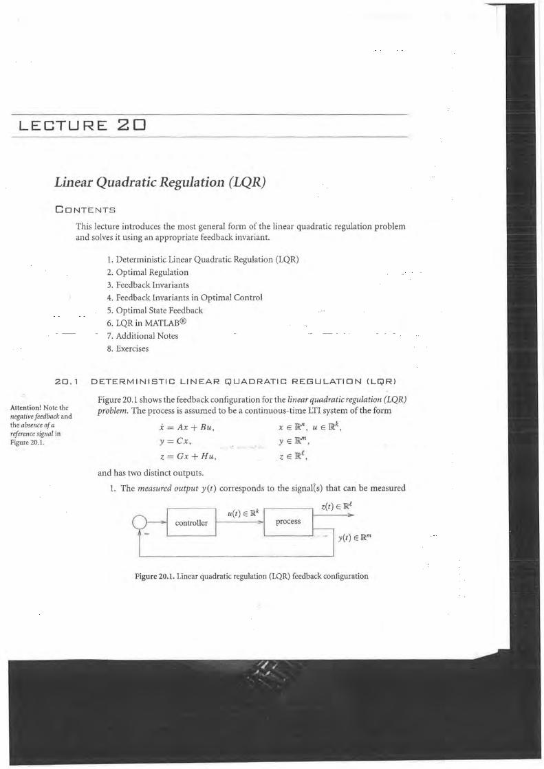
Figure 20.1 shows the feedback configuration for the linear quadratic regulation (LQR) problem. The process is assumed to be a coritinuous-time LTl system of the form

x = Ax + Bu,

y =Cx,

z = Gx + Hu,

and has two distinct outputs.

x E jRn, U E jRk,

Y E jRm,

_Z E jRe,

1. The measured output yet) corresponds to the signal(s) that ca~ be measured

u(t) E ]Rk Z

C)---- controller process I--

(t) E]Rl

- _0 y(t)

Figure 20.1. Linear quadratic regulation (LQR) feedback configuration

192

Note. Measured outputs are typically determined by the availab le sensors.

Note. Contro lled outputs are selec ted by the controller designer and should be viewed as design parameters.

LECTURE 20

and are therefore available for control.

2. The controlled output z(t) corresponds to the signal(s) that one would like to

make as small as possible in the shortest possible time.

Sometimes z(t) = yet) , which means that our control objective is simply to make the measured output very small. At other times one may have

[yet)]

z(t) = yet) ,

which means that we want to make both the measured output yet) and its derivative Yet) very small. Many other options are possible.

20.2 OPTIMAL REGULATION

Note 11. A simple choice fo r the matrices Q and R is given by Bryson's rule. ~ p. 196

The LQR problem is defined as follows. Find the control input u(t) , t E [0,00) that makes the following criterion as small as possible:

(20.1)

where p is a positive constant. The term

corresponds to the energy of the controlled output, and the term

corresponds to the energy of the control signal. In LQR one seeks a controller that minimizes both energies. However, decreasing the energy of the controlled output will require a large control signal, and a small control signal will lead to large con­trolled outputs. The role of the constant p is to establish a trade-off between these conflicting goals.

1. When we chose p very large, the most effective way to decrease hQR is to employ a small control input, at the expense of a large controlled output.

2. When we chose p very small, the most effective way to decrease hQR is to obtain a very small controlled output, even if this is achieved at the expense of employing a large control input.

Often the optimal LQR problem is defined more generally and consists of finding the control input that minimizes

hQR := 1000

z(t)' Qz(t) + p u(t)' Ru(t) dt , (20.2)

r LINEAR QUADRATIC REGULATION (LQR) 193

where Q E JR.exe and R E JR.m xm are symmetric positive-definite matrices and p is a positive constant.

We shall consider the most general form for a quadratic criterion, which is

hQR:= la oo x(t)' Qx(t) + u(t)' Ru(t) + 2x(t)' Nu(t)dt. (J-LQR)

Since z = Gx + H u, the criterion in (20.1) is a special form ofthe criterion (J-LQR) with

Q = G'G, R = H'H+pI, N=G'H

and (20.2) is a special form of the criterion (J-LQR) with

Q = G'QG, R=H'QH+pR, N=G'QH.

20.3 FEEDBACK INVARIANTS

Note. A functional maps functions (in this case signals, i.e. functions of time) to scalar values (in this case real numbers).

Note. This concept was already introduced in Lecture 10, where Proposition 20.1 was proved. ~p.88

Given a continuous-time LTI system

x = Ax + Bu, (AB-CLTI)

we say that a functional

H(xO; uO)

that involves the system's input and state is a feedback invariant for the system (AB­CLTI) if, when computed along a solution to the system, its value depends only on the initial condition x(O) and not on the specific input signal uO.

Proposition 20.1 (Feedback invariant). For every symmetric matrix P, the functional

H(x(.); liO) := - la oo (Ax(t) + Bu(t»)' Px(t) + x(t)'P(AX(t) + B:Ct)) dt

is a feedback invariant for the system (AB-CLTI), as long as lim/-+oo x(t) = O. 0

20.4 FEEDBACK INVARIANTS IN OPTIMAL CONTROL

Suppose that we are able to express a criterion J to J;>e minimized by an appropriate choice of the input u(·) in the form

J = H(x( .); uO) + la oo A(x(t), u(t»)dt, (20.3)

where H is a feedback invariant and the function A(x, u) has the property that for every x E JR.n

min A(x, u) = O. UElRk

194

Note. If one wants to restrict the optimization to solutions that lead to an asym ptotically stable dosed-loop system. then H needs to be a feedback invariant only for inputs that lead to x(t) ->- 0 (as in Proposition 20.1). However. in this case one must check that (20.4) does indeed lead to X(I) ->- O.

20.5

Attention! To keep the formulas short. in the remainder of this section we drop the time dependence (I) when the state x and the input u appear in time integrals.

In this case, the control

u(t) = arg min1\(x, u), uElRk

LECTURE 20

(20.4)

minimizes the criterion J, and the optimal value of J is equal to the feedback invari­ant

J = H(xO; uO).

Note that it is not possible to get a lower value for J, since (1) the feedback invariant H(xO; u(.») will never be affected by u, and (2) a smaller value for J would require the integral in the right-hand side of (20.3) to be negative, which is not possible, since 1\ (x (t), u(t») can at best be as low as zero.

OPTIMAL STATE FEEDBACK

It turns out that the LQR criterion

hQR := 1000

x(t)' Qx(t) + u(t)' Ru(t) + 2x(t)' Nu(t)dt (J-LQR)

can be expressed as in (20.3) for an appropriate choice of feedback invariant. In fact, the feedback invariant in Proposition 20.1 will work, provided that we choose the matrix P appropriately. To check that this is so, we add and subtract this feedback invariant to the LQR criterion and conclude that

hQR:= 1000

x' Qx + u'Ru + 2x' Nu dt

= H(x( .); uO)

+ 1000

x' Qx +u'Ru + 2x' Nu + (Ax + Bu)' Px + x' P(Ax + Bu) dt

= H(x( .); uO) + 1000

x'(A' P + P A + Q)x + u'Ru + 2u'(B' P + N')x dt.

By completing the square, we can group the quadratic term in u with the cross-term in u times x:

(u' + x' K')R(u + Kx)

= u'Ru + x ' (P B + N)R- 1 (B' P + NI)x + 2u l (BI P + N')x,

where

from which we conclude that

hQR = H(x(.); uO) + 1000

x'(A' P + PA + Q - (PB + N)R-1(B' P + N'»)x

+ (u' + x' K')R(u + Kx) dt.

'.

LINEAR QUADRATIC REGULATION (LQR) 195

Notation. Equation (20.5) is called an algebraic Riccati equation (ARE).

Notation. Recall that a matrix is Hurwitz or a stability matrix if all its eigenvalues have a negative real part.

Note. Asymptotic stability of the closed loop is needed, beca use we need to make sure that the proposed input u (t) leads to the assumed fact tha t liml--+oo X(I) P x(t) = o.

MATLAB® Hint 42. lqr solves the ARE (20.5) and computes the optimal state feedback (20.6) . ~ p. 195

If we are able to select the matrix P so that

A' P + PA + Q - (PB + N)R- 1(B' P + N') = 0, (20.5)

we obtain precisely an expression such as (20.3) with

A(x, u) := (u' + x' K')R(u + Kx),

which has a minimum equal to zero for

u = -Kx,

leading to the closed-loop system

i = (A - BR- 1(B' P + N'»)x.

The following has been proved.

Theorem 20.1. Assume that there exists a symmetric solution P to the algebraic Ric­cati equation (20.5) for which A - BR- 1(B' P + N') is a stability matrix. Then the feedback law

u(t) := -Kx(t), Vt:::: 0, (20.6)

minimizes the LQR criterion (J-LQR) and leads to

hQR := 1000

x' Qx + u'Ru + 2x' Nu dt = x'(O)Px(O). o

20.6 LQR IN MATLAS®

Example. See Example 22.1.

MATLAB® Hint 42 (lqr). The command [K , P, EJ =lqr (A, B I Q I R, N) solves the algebraic Riccati equation

A'P + PA+ Q - (PB + N)R - 1(B'P + N') = 0

and computes the (negative feedback) optimal state feedback matrix gain

K = R- 1(B'P + N')

that minimizes the LQR criteria

J := 1000

x'Qx + u'Ru + 2x'NU dt

for the continuous-time process

X =Ax +Bu .

This command also returns the poles E of the closed-loop system

x = (A - BK)x. o

196 LECTURE 20

20.7 ADDITIONAL NOTES

Note 11 (Bryson's rule). A simple and reasonable choice for the matrices Q and R in (20.2) is given by Bryson's rule [6, p. 537]. Select Q and R diagonal, with

- 1

Q;; = maximum acceptable value of zr' iE{1,2, ... ,E},

- 1 R j j = 2'

maximum acceptable value of U j j E {I, 2, . . . , k},

which corresponds to the following criterion

In essence, Bryson's rule scales the variables that appear in hQR so that the maximum acceptable value for each term is 1. This is especially important when the units used for the different components of u and z make the values for these variables numerically very different from each other.

Although Bryson's rule usually gives good results, often it is just the starting point for a trial-and-error iterative design procedure aimed at obtaining desirable proper­ties for the dosed-loop system. We shall pursue this further in Section 22.3. 0

20.8 EXERCISES

20.1 (Feedback invariant). Consider the nonlinear system

i = I(x, u) ,

and a continuously differentiable function V : JRn -+ JR, with V (0) = O. Verify that the functional . . - .

l°o av

H(x(.); uO) := - - (x(t) )/(x(t), u(t») dt o ax

is a feedback invariant as long as limt-+oo x(t) = O. o 20.2 (Nonlinear optimal control). Consider the nonlinear system

i = I(x , u),

Use the feedback invariant in Exercise 20.1 to construct a result parallel to Theo­rem 20.1 for the minimization of the criterion

J :=100 Q(x) + u'R(x)u dt,

where R(x) is a state-dependent positive-definite matrix. o

LECTU RE 2 1

The Algebraic Riccati Equation (ARE)

CONTENTS

This lecture addresses the existence of solutions to the algebraic Riccati equation.

1. The Hamiltonian Matrix

2. Domain of the Riccati Operator

3. Stable Subspaces

4. Stable Subspace of the Hamiltonian Matrix

5. Exercises

21.1 THE HAMILTONIAN MATRIX

The construction of the optimal LQR feedback law in Theorem 20.1 required the existence of a symmetric solution P to the ARE,

A' P + P A + Q - (P B + N) R- 1 (B ' P + N ' ) = 0, (21.1 )

for which A - B R-1 (B' P + N') is a stability matrix. To study the solutions of this equation, it is convenient to expand the last term in the left-hand side of (21.1), which leads to

(A - BR- 1 N ' ).' P + peA - BR - 1N' ) + Q - N R- 1 N ' - P BR - 1 B' P = o. (21.2)

This equation can be compactly rewritten as

(21.3)

where

is called the Hamiltonian matrix associated with (21.1).

198

21 .2

Notation. We write H E Ric when H is in the domain of the Riccati operator.

Notation. In general the ARE has multiple solutions, but only the one in (21.4) makes the closed-loop system asymptotically stable. This solution is called the stabilizing solution.

Note. We shall confirm in Exercise 21.1 that the matrix in the left-hand side of (21.5) is indeed symmetric.

Note. This same argument was used in the proof of the Lyapunov stability theorem (Theorem 8.2).

LECTURE 21

DOMAIN OF THE RICCATI OPERATOR

A Hamiltonian matrix H is said to be in the domain of the Riccati operator if there exist square matrices H_, P E jRnxn such that

HM = MH_ , M'= [I] . p' (21.4)

where H_ is a stability matrix and I is the n x n identity matrix.

Theorem 21.1. Suppose that H is in the domain of the Riccati operator and let P, H_ E

jRnxn be as in (21.4). Then the following properties hold.

1. P satisfies the ARE (21.1),

2. A - B R- 1 (B I P + N I) = H_ is a stability matrix, and

3. P is a symmetric matrix. o

Proof of Theorem 21.1. To prove statement 1, we left-multiply (21.4) by the matrix [p - I] and obtain (21.3).

To prove statement 2, we just look at the top n rows of the matrix equation (21.4):

from which A - BR-\B I P + N I) = H_ follows.

To prove statement 3, we left-multiply (21.4) by [ - pi I] and obtain

[_pi r] H [~J = (P - P')H_. '. (21.5)

Moreover, using the definition of H, we can conclude that the matrix in the left-hand side of (21.5) is symmetric. Therefore

(P - P')H_ = H~(pl - P) = -H~(P - p\ (21.6)

Multiplying this equation on the left and right byeR.:t and eH- t , respectively, we conclude that

eH~t (P _ P')H_e H- t + eH~IH~ (P - pl)eH- 1 = 0

{} :t eH~t (P - pl)eH_t = 0,

\It, which means that eH~t (P - pl)eH_t is constant. However, since H....: isa stability matrix, this quantity must also converge to zero as t --+ 00. Therefore it must actually be identically zero. Since eH _ t is nonsingular, we conclude that we must have P = pl. •

THE ALGEBRAIC RICCATI EQUATION (ARE) 199

21.3 STABLE SUBSPACES

Note. See Exercise 21.3.

Note. From P21.1, we can see that the dimension of V_ is equal to the number of eigenvalues of M with a negative real part (with repetitions) .

21 . 4

Given a square matrix M, suppose that we factor its characteristic polynomial as a product of polynomials

where all the roots of .0.-Cs) have a negative real part and all roots of t.+Cs) have positive or zero real parts. The stable subspace of M is defined by

v _ := ker .0.-CM)

and has a few important properties, as listed below.

Properties (Stable subspaces). Let V_be the stable subspace of M. Then

P21.1 dim V_ = deg .0._Cs), and

P21.2 for every matrix V whose columns form a basis for V _, there exists a stability matrix M_ whose characteristic polynomial is .0.-Cs) such that

(21.7)

STABLE SUBSPACE OF THE HAMILTONIAN MATRIX

Our goal now is to find the conditions under which the Hamiltonian matrix H E

JR.2nx2n belongs to the domain of the Riccati operator, i.e., those for which there exist

symmetric matrices H_, P E JR.nxn such that

HM=MH_,

- . where H_ is a stability matrix and I is the n x n identity matrix. From the properties of stable subspaces, we conclude that such a matrix H_ exists if we can find a basis for the stable subspace V_of H of the appropriate form M = [I pI]'. For this to be possible, the stable subspace has to have dimension precisely equal to n, which is the key issue of concern. We shall see shortly that-the .structure .[I pI]' for Mis, relatively simple to produce.

21.4.1 DIMENSION OF THE STABLE SUBSPACE OF H

To investigate the dimension of V _, we need to compute the characteristic polyno­mial ofH. To do this, note that

H[ 0 -I

I] [ BR-1BI

o = CA - BR-1N')' -I] HI o .

Therefore, defining J := [..?[ 6],

H= -JH'J-1 •

. '

~

I

200

Notation. The symbol (.)* denotes complex conjugate transpose.

Attention! The notation used here differs from that of MATLAB®. Here 0' denotes transpose and (.)* denotes complex conjugate transpose, whereas in MATLAB®, (.) .' denotes transpose and (.) , denotes complex conjugate transpose.

LECTURE 21

Since the characteristic polynomial is invariant with respect to similarity transforma­tions and matrix transposition, we conclude that

6.(s) := det(sl - H) = det(sl + JHI J-I) = det(sl + HI)

= det(s 1 + H) = (_1)2n det« -s)1 - H) = 6.( -s),

which shows that if A is an eigenvalue of H, then - A is also an eigenvalue of H with the same multiplicity. We thus conclude that the 2n eigenvalues ofH are distributed symmetrically with respect to the imaginary axis. To check that we actually have n eigenvalues with a negative real part and another n with a positive real part, we need to make sure that H has no eigenvalues over the imaginary axis. This point is addressed by the following result.

Lemma 21.1. Assume that Q - N R- I N I :::: O. When the pair (A, B) is stabilizable and the pair (A - BR-INI, Q - NR-IN/) is detectable, then

1. the Hamiltonian matrix H has no eigenvalues on the imaginary axis, and

2. its stable subspace V_has dimension n. o

Attention! The best LQR controllers are obtained for choices of the controlled output z for which N = GI H = 0 (cf. Lecture 22). In this case, Lemma 21.1 simply requires stabilizability of (A, B) and detectability of (A, G) (cf. Exercise 21.4). 0

Proof of Lemma 21.1. To prove this result by contradiction, let x : = [x~ x~]', XI, X2 E en be an eigenvector of H associated with an eigenvalue A := jw, w E lR. This means that

[jWI - A + BR- I N I

Q - NR-IN I BR-

I BI ] [Xl] _ 0

jw+(A-BR-IN/)1 X2 - . (21.8)

Using the facts that (A, :XYi~ '~~ 'eigenvalue/eigenvectoi pair ofH and that"this matrix is real-valued, one concludes that

[X~ Xn H [~~] + [xt x~] HI [~~]

= [x~ xn (Hx) + (Hx)* [~~]

(21.9)

On the other hand, using the definition of H, one concludes that the left-hand side of (21.9) is given by

r THE ALGEBRAIC RICCATI EQUATION (ARE) 201

[(A - BR-IN')'

+ [X *I X*] 2 -BR-IB'

Since this expression must equal zero and R- I > 0, we conclude that

(Q - N R- I N')xI = 0, B'X2 = o.

From this and (21.8) we also conclude that

(jwl - A + BR- I N')xI = 0, (jw + A')X2 = o.

But then we have an eigenvector X2 of A' in the kernel of B' and an eigenvector XI of A - BR- I N' in the kernel of Q - N R- 1 N'. Since the corresponding eigenvalues do not have negative real parts this con tradicts the stabilizability and detectability assumptions.

The fact that V_has dimension n follows from the discussion preceding the state­ment of the lemma. •

21.4.2 BASIS FOR THE STABLE SUBSPACE OF H

Note. Under the assumptions of Lemma 21.1, VI is always nonsingular, as shown in [5, Theorem 6.5, p. 202).

Suppose that the assumptions of Lemma 21.1 hold and let

V := [~~J E ~2n x n

be a matrix whose n columns form a basis for the stable subspace V_of H. Assuming that VI E jRnxn is nonsingular, then

VV- I = [I] I p'

is also a basis for V _. Therefore, we conclude from property P21.2 that there exists a stability matrix H_ such that

(21.10)

and therefore H belongs to the domain of the Riccati operator. Combining Lemma 21.1 with Theorem 21.1, we obtain the following main result regarding the solution to the ARE.

Theorem 21.2. Assume that Q - N R-1 N' 2': O. Vi'hen the pair (A, B) is stabilizable and the pair (A - B R-1 N' , Q - N R- I N') is detectable,

1. H is in the domain of the Riccati operator,

2. P satisfies the ARE (21.1),

202

Note 12. When the pair (A - BR-IN', Q­NR - 1N') is observable, one can show that P is also positive­definite. ~ p. 202

LECTURE 21

3. A - B R- I (B' P + N') = H_ is a stability matrix, and

4. P is symmetric,

where P, H_ E IRnxn are as in (21.10). Moreover, the eigenvalues ofH- are the eigenvalues ofH with a negative real part. 0

Attention! It is insightful to interpret the results of Theorem 21.2, when applied to the minimization of

hQR:= 100Z'QZ+PU'Rudt, z:=Gx+Hu, p,Q,R>O,

which corresponds to

Q = G'QG, R = H'QH +pR, N = G'QH.

When N = 0, we conclude that Theorem 21.2 requires the detectability of the pair (A, Q) = (A, G' QG). Since Q > 0, it is straightforward to verify (e.g., using the eigenvector test) that this is equivalent to the detectability of the pair (A, G), which means that the system must be detectable through the controlled output z.

The need for CA, B) to be stabilizable is quite reasonable, because otherwise it is not possible to make x -+ 0 for every initial condition. The need for (A, G) to be detectable can be intuitively understood by the fact that if the system had unstable modes that did not appear in z, it could be possible to make hQR very small, even though the state x might be exploding. 0

Note 12. To prove that P is positive-definite, we rewrite the ARE

(A - BR- 1 N')' P + peA - BR- 1 N') + Q - N R- I N' - P BR- 1 B' P = 0

in (21.2) as

H~P + PH_ = -S, S:= (Q - NR-1N') + PBR-IB' P.

The positive definiteness of P then follows from the Lyapunov observability test as long as we are able to establish the observability of the pair (H_, S).

To show that the pair (H_, S) is observable, we use the eigenvector test. To prove this by contradiction, assume that x-is an ·eigenvector.ofH_ that lies in the kernel of S; i.e.,

Since Q - N R- 1 N' and P B R-1B' P are both symmetric positive-semidefinite ma­trices, the equation Sx = 0 implies that

x'((Q-NR-1N')+PBR-1B'P)x=0::::} (Q-NR-1N')x=0, B'px=O.

We thus conclude that

(A - BR- 1 N')x = Ax,

which contradicts the fact that the pair (A - B R- 1 N', Q - N R-1 N') is observable. o

THE ALGEBRAIC RICCATI EQUATION (ARE) 203

21.5 EXERCISES

21.1. Verify that for every matrix P, the following matrix is symmetric:

where H is the Hamiltonian matrix. 0

21.2 (Invariance of stable subspaces). Show that the stable subspace V_of a matrix M is always M-invariant. 0

21.3 (Properties of stable subspaces). Prove Properties P21.1 and P21.2.

Hint: Transform M into its Jordan normal form. o 21.4. Show that detectability of (A, G) is equivalent to detectability of (A, Q) with Q:=G'G.

Hint: Use the eigenvector test and note that the kernels of G and G' G are exactly the m~ 0

LECTURE 22

Frequency Domain and Asymptotic Properties of LQR

CONTENTS

This lecture discusses several important properties of LQR controllers.

1. Kalman's Equality

2. Frequency Domain Properties: Single-Input Case

3. Loop Shaping using LQR: Single-Input Case

4. LQR Design Example

5. Cheap Control Case

6. MATLAB® Commands

7. Additional Notes

8. The Loop-shaping Design Method (review)

9. Exercises

22.1 KALMAN'S Ec;JUALITY

Attention! This condition is /lot being added for simplicity. We shall see in Example 22.1 that, without it, the results in this section are not valid.

Consider the continuous-time LTI process

i = Ax + Bu, z=Gx+Hu,

for ~hich one wants to minimize th~ LQR crite.~io,n

hQR := 100

Ilz(t)11 2 + pllu(t)1I2

dt,

where p isa positive constant. Throughout this whole lecture we assume that

N:= G'H =0,

for which the optimal control is given by

u = -Kx, K:=R- 1B'P, R:= H'H +pl,

where P is the stabilizing solution to the ARE

A'P + PA + G'G - PBR- 1 B'P = o.

(22.1 )

(22.2)

FREQUENCY DOMAlN AND ASYMPTOTIC PROPERTIES OF LQR 205

Note. Kalman's equality follows directly from simple algebraic manipulations of the ARE (cf. Exercise 22.1).

u

x=Ax+Bu

x

Figure 22.1. State feedback open-loop gain.

We saw in the Lecture 20 that under appropriate stabilizability and detectability as­sumptions, the LQR control results in a closed-loop system that is asymptotically stable.

LQR controllers also have desirable properties in the frequency domain. To under­stand why, consider the open-loop transfer matrix from the process input u to the controller output u (Figure 22.1). The state-space model from u to u is given by

i = Ax + Bu , u = -Kx,

which corresponds to the following open-loop negative-feedback k x k transfer matrix

L(s) = KCsI - A)-l B.

Another important open-loop transfer matrix is that from the control signal u to the controlled output z,

T(s) = G(sI - A)-l B + H.

These transfer matrices are related by the so-called Kalman's equality:

Kalman's equality. For the LQR criterion in (22.1) with (22.2), we have

(I + LC-s)')R(I + £(s») =R + H'H + T(-s)'Tcs). (22.3)

Kalman's equality has many important consequences. One of them is Kalman's inequality, which is obtained by setting s = jw in (22.3) and using the fact that for real-rational transfer matrices

£(-jw)' = L(jw)*, TC-jw)' = T(jw)*, H'H + T(jw)*T(jw)::: O.

Kalman's inequality. For the LQR criterion in (22.1) with (22.2), we have

(22.4)

22.2 FRE4IUENCY DOMAIN PROPERTIES: SINGLE-INPUT CASE

We focus our attention in single-input processes (k = 1), for which £(s) is a scalar transfer function. Dividing both sides of Kalman's inequality (22.4) by the scalar R, we obtain

Note 13. For multiple input systems, similar conclusions could be drawn, based on the multivariable Nyquist criterion. ~ p. 216

which expresses the fact that the Nyquist pIal of i(jev) does not enter a circle of ra­dius 1 around the point -1 of the complex plane. This .is represented graphically in Figure 22.2 and has several significant implicllLi.0ns, which arc discussed next.

r

206

Note. The first inequality results directly from the fact

that 11 + L(jw)1 2: I, the second ftdm the -fact that T(s) = 1 - S(s), and the last two from the fact that the second inequality shows that T(jw) must belong to a circle of radius 1 around the point + 1.

LECTURE 22

Re

Figure 22.2. Nyquist plot for a LQR state feedback controller.

POSITIVE GAIN MARGIN . If the process gain is multiplied bya constant k > 1, its Nyquist plot simply expands radially, and therefore the number of encirclements does not change. This corresponds to a positive gain margin of +00.

NEGATIVE GAIN MARGIN. If the process gain is multiplied by a constant 0.5 < k < 1, its Nyquist plot contracts radially, but the number of encirclements still does not change. This corresponds to a negative gain margin of20 log 10 (.5) = -6 dB.

P HAS E MAR GIN. If the process phase increases bye E [- 60°,60°], its Nyquist plot rotates bye, but the number of encirclements still does not change. This corre­sponds to a phase margin of ±60°.

SENSITIVITY AND COMPLEMENTARY SENSITIVITY FUNCTIONS. The sensitivity and the complementary sensitivity functions are given by

A 1 S(s) := A,

1 + L(s)

£(s) T(s) := 1 - S(s) = ---:---

1 + L(s)

respectively. Kalman's inequality guarantees that

IS(jev) I :::: 1, IT(jev) - 11 :::: 1, IT(jev)l:::: 2, m[T(jev)]:::: 0, "lev E IR.

(22.5)

We recall the following facts about the sensitivity function.

1. A small sensitivity function is desirable for good disturbance rejection. Gener­ally, this is especially important at low frequencies.

2. A complementary sensitivity function close to 1 is desirable for good reference tracking. Generally, this is especially important at low frequencies.

3. A small compleinentary sensitivity function is "desirable for good noise rejec­tion. Generally, this is especially important at high frequencies.

FREQUENCY DOMAIN AND ASYMPTOTIC PROPERTIES OF LQR 207

Note. If the transfer function from u to y has two more poles than zeros, then one can show that C B = 0 and H = O.

Attention! Kalman's inequality is valid only when N = G' H = O. When this is not the case, LQR controllers can exhibit significantly worse properties in terms of gain and phase margins. To some extent, this limits the controlled outputs that should be placed in z. For example, consider the process i = Ax + Bu, y = Cx and suppose that we want to regulate

z = y = Cx.

This leads to G = C and H = O. Therefore G' H = 0, for which Kalman's inequality holds. However, choosing

leads to

and therefore In this case, Kalman's inequality holds also G' H = A' C' C B, for this choice of z.

22.3

Note. Loop shaping consists of designing the controller to meet specifications on the open'-loop gain -L(s). A brief review of this control design method can be found in Section 22.8.

MATLAB® Hint 43. sigma (sys) draws the norm-Bode plot of the system sys. ~ p. 216

which may not be equal to zero. 0

LOOP SHAPING USING LQR: SINGLE-INPUT CASE

Using IVllman's inequal.iLy, we saw that any LQR controller automatically provides some upper bounds on the magnitude of the sensitivity function and its comple­mentary. However, UJese bounds are frequency-independent and may not result in appropriate loop shaping.

We discuss next a few rules that allow us to perform loop shaping using LQR. We continue to restrict our attention to the single-input case (k = O.

LOW-FREC<JUENCY OPEN-LOOP GAIN. Dividing both sides of Kalman's equality (22.3) by the scalar R:= H' H + p, we obtain

H' H IIT( 'UJ)11 2 11 + L( 'UJ)1 2 = 1 + + _...:...1 __

1 H'H+p / H'H+p

Therefore, for the range of frequencies for which IL(jUJ) I » 1 (typically low fre­quencies),

which means that the open-loop gain for the optimal feedback L(s) follows the shape of the Bode plot from u to the controlled output z. To understand the implications of this formula, it is instructive to consider two fairly typical cases.

208

Note. Although the magnitude of L(jw) mimics the magnitude ofT(jw), the phase of the open-loop gain LUw) always leads to a stable closed loop with an appropriate phase margin.

LECTURE 22

1. When z = y, with y := Cx scalar, we have

where

is the transfer function from the control input u to the measured output y. In this case,

(a) the shape of the magnitude of the open-loop gain L(jw) is determined

by the magnitude of the transfer function from the control input u to the measured output y, and

(b) the parameter p moves the magnitude Bode plot up and down (more precisely H' H + p).

2. When z = [y yy J', with y := Cx scalar, i.e.,

we conclude that

A [ P(S)] [ 1 ] A res) = A = pes), ys pes) ys

and therefore

pes) := C(sl - A)-I B,

11 + jywIIP(jw)1

,JH'H + p (22.6)

In this case, the low-frequency open-loop gain mimics the process transfer function from u to y, with an extra zero at l/y and scaled by ~. Thus

H'H+p

(a) p moves the magnitude Bode plot up and down (more precisely H' H + p), and

(b) large values for y lead to a low-frequency zero and generally result in a larger phase margin (above the minimum of 60°) and a smaller overshoot in the step response. However, this is often achieved at the expense of a slower response.

FREQUENCY DOMAIN AND ASYMPTOTIC PROPERTIES OF LQR 209

Attention! It sometimes happens that the above two choices for z still do not pro­vide a sufficiently good low-frequency open-loop response. In such cases, one may actually add dynamics to more accurately shape L(s). For example, suppose that one wants a very large magnitude for L (s) at a particular frequency Wo to reject a specific periodic disturbance. This could be achieved by including in z a filtered version of the output y obtained from a transfer function with a resonance close to Wo to increase the gain at this frequency. In this case, one could define

z = [~~] , Y2Y

where ji is obtained from y through a system with transfer function equal to

for some small E > O. Many other options are possible, allowing one to precisely shape L(s) over the range of frequencies for which this transfer function has a large magnitude. 0

HIGH-FRE~UENCY OPEN-LOOP GAIN. Figure 22.2 shows that the open-loop gain L(jw) can have at most -900 phase for high-frequencies, and therefore the roll-off rate is at most -20 dB/decade. In practice, this means that for w » 1,

~ c IL(jw)l~ w.JH'H+p'

for some constant c. Therefore the cross-over frequency is approximately given by

Thus

c --:~~=~1 wcross.J H' H + p

C

Wcross ~ JH'H + p'

1. LQR controllers always exhibit a high-frequency magnitude decay.of -20 dB/ decade, and

2. the cross-over frequency is proportional to 1/ J H' H + p, and generally small values for H' H + p result in faster step responses.

Attentionl The (slow) -20 dB/decade magnitude decrease is the main shortcoming of state feedback LQR controllers, because it may not be sufficient to clear high­frequency upper bounds on the open-loop gain needed to reject disturbances and/or for robustness with respect to process uncertainty. We will see in Section 23.5 that this can actually be improved with output feedback controllers. 0

210 LECTURE 22

22.4 LQR DESIGN EXAMPLE

MATLAB® Hint 44. See MATLAB®Hint 42. ~p. 195

Example 22.1 (Aircraft roll dynamics). Figure 22.3 shows the roll angle dynamics of an aircraft [15, p. 381]. Defining x := [8 w r]', we can write the aircraft dynamics as

where

-0.875 o

x = Ax + Bu,

o PEN-LO 0 P GAl N s. Figure 22.4 shows Bode plots of the open-loop gain L(s) = K (s I - A) - l B for several LQR controllers obtained for this system. The controlled output was chosen to be z := [8 ye]', which corresponds to

G:= [~ o y fI := [~J .

The controllers minimize the criterion (22.1) for several values of p and y. The matrix gains K and the Bode plots of the open-loop gains can be computed using the following sequence of MATLAB®commands:

A [0,1,0;0,-.875,-20;0,0,-50];

G [l,O,O;O,gamma*l,O] ;

Q G' *G; R = H' *H+rho;

K=lqr(A,B,Q,R,N) ;

GO=ss (A, B, K, 0) ;

bode(GO) ;

B

H

N

[0; 0; 50] ;

% process dynamics [0; 0] ;

% controlled output z G'*H; % weight matrices % compute LQR gain % open-loop gain'

___ .. ___ fQr 1h~.differ~nt y'alq~s_of ga,mrn~ __ ,!-n~_~r-0"

T applied torque

Figure 22.3. Aircraft roll angle dynamics.

e=w w = -0.875w - 20r

i = -50r +50u

FREQUENCY DOMAIN AND ASYMPTOTIC PROPERTIES OF LQR 211

Note. The use of LQR .. , controllers to drive an

output variable to a set point will be studied in detail later in Section 23.6.

100fj'El<: ' . "W~~"'~'

OOJ"" ' ~, lG""" . in "''''';~~~,'h~ .• ~ 0 -JQ~~~~~~ •. .~ -50 - - . P(s) from u to a J ~~~~_11 ~ -100 .-<c)- L(s) lory • • 01, p. 01

~L(s)lor.,=.01,p=1 ...... - fSO ~_~ LI&) IOrT= ,Ot P = 100

10' 10'

-BO I-~~--""----~--

-100 ~"':~,"-,..ti' iI*',# ." .-i ... .. 't~ , ... U fJ :!-~,;

i-120 :," ~1)'y..-0/· . "'\ .. ,

a-140 " -~~'.: \.

-l S0

10° 10t frequency (fad'sJ

..J

10'

ro'

10'

(a) Open-loop gain for several values of p. This parameter allows us to move the whole magnitude Bode plot up and down.

1:'iS_~~_=_~~-._ ~'_~, _~' 11 - ' - P(s) Irom u 10 B ::3'

... j L(s)forp= .01.y", .01 ... , -: ~L(s) lorp= 01,y= 1

-!!-- Lt~l ror p = 01 , T= 3

-80

-100 -

~ ~ -1 20

~ -a -140

-!(j(J

10-2 10·t 10° 10' 102 103

rrequency [fad/sJ

(b) Open'loop gain for several values of y. Larger values for this parameter result in a larger phase margin.

Figure 22.4. Bode plots for the open-loop gain of the LQR controllers in Example 22. L As ex­pected, for low frequencies the open-loop gain magnitude matches that ofthe process transfer function from u to e (but with significantly lower/better phase), and at high-frequencies the gain magnitude falls at -20 dB/decade.

Figure 22A(a) hows the open-I.oop {,rain for several values of p, where we CRn sec that p al lows us t mov the wh01e magnitude Bode plot up and down. Figure 22.4(h) shows the open- loop gain for several va lues of y, where we an see that a larger )I

results in a larger phase margin. As expected, for low frequencies the open-loop gain magnitude matches that of the process transfer runction hom u lo. () (hul with significantly lower/better f hase), and at high frequencies the gain magnitude fa lls at - 20 dB/decade.

STEP RES PO N S ES. Figure 22.5 shows step responses for the state feedback LQR controllers whos~ Bode plots for the open-loop gain are shown in figure 22.4 . Figure 22.5(a) shows that smaller values of p lead to faster responses, and Figure 22.5(b) shows that larger values for y lead to smaller overshoots (but slower re­sponses).

NYQU 1ST PLOTS. Figure 22.6 shows Nyquist plots of the open-loop gain L(s) = K(sI - A)-lB for p = 0.01, but different choices of the controlled output z. In Figure 22.6(a) z := [e OJ', which corresponds to

212

1.4~-~--~----~-~--~

1,2

, (-':~ 0 ,6 , -

I 0.6 ,

I 0.4 I

0,2 , , I J

o ' o

[

--Y= 01,P= .01J - - - Y = 01 P = 1

- P 01 01' = 100

2 3 Urn.

(a) Step response for several values of p. This parameter allows us to control the speed of the response.

LECTURE 22

1.4r---~--~-~--~---~

12

l ' f;-:-.---- - ~-I _,-

06 I

0.61 f,/ --

0.4 11

r- p = ·Ol,Y= 01

0,2

3 time

- - -p= .Ol,y= .l -- - p= 01,y= 3

(b) Step response for several values of y. This parameter allows us to control the overshoot.

Figure 22.5. Closed-loop step responses for the LQR controllers in Example 22.1.

In this case, H' G = [0 0 0], and Kalman's inequality holds, as can be seen in the Nyquist plot. In Figure 22.6(b), the controlled output was chosen to be z := [e i: J', which corresponds to

G:= [~ o o

In this case, we have H' G = [00 -2500], and Kalman's inequality does not hold. We can see from the Nyquist plot that the phase and gain margins are very small and there is little robustness with respect to unmodeled dynamics, since a small perturbation in the process can lead to an encirclement of the point -1. 0

:~----l 3,

phase merom .. 72.8 ~

P"IISI>!MllIln • 9,S

~ ~ 0 -Z '

'~

~ -1 -1

-2 -?

-3 ~----~-~-~--------~ -3 -~ -3 -2 -1 -4 -3 -2 -1

real axis real axis

(a) G'H =0 (b) G'H #0

Figure 22.6. Nyquist plots for the open-loop gain of the LQR controllers in Example 22.l.

FREQUENCY DOMAIN AND ASYMPTOTIC PROPERTIES OF LQR 213

22.5 CHEAP CONTROL CASE

In view of the LQR criterion

by making p very small one does not penalize the energy used by the control signal. Based on this, one could expect that, as p --+ 0,

1. the system's response becomes arbitrarily fast, and

2. the optimal value of the criterion converges to zero.

This limiting case is called cheap control and it turns out that whether or not the above conjectures are true depends on the transmission zeros of the system.

22.5.1 CLOSED-LOOP POLES

Note. Cf. Exercise 22.2.

Note. The transfer matrix r(s) that appears in (22.7) can be viewed as the transfer function from the control input u to the controlled output z.

We saw in Lecture 21 (cf. Theorem 21.2) that the poles of the closed loop correspond to the stable eigenvalues of the Hamiltonian matrix

[A -BR-1 BIJ m2nx2n

H:= -G'G -A' E IN>. ,

To determine the eigenvalues ofH, we use the fact that

det(s I - H) = ct..(s)t..( -s) det (R - H' H + 1'( -S)'f(S»), (22.7)

where c := (_l)n det R- 1 and

t..(s) := det(sl - A), 1'(s) := G(sI - A)-IB + H.

As P --+ 0, H' fI -~ R, and i:h-eretore

det(sI - H) --+ ct..(s)t..(-s)detT(-s)'1'(s). (22.S)

We saw in Theorem lS.2 that th~re exist unimodular real polyno~ialmatrices L(s) E JR[s]eXe, R(s) E JR[s]kxk such that - - - - -- -- - --- -- -

where

1'(s) = L(s)SMr(s)R(s),

o

I1r(S) 1/fr{S)

o 000:']

(22.9)

E JR(s)exk

is the Smith-McMillan form of l' (s). To proceed, we should consider the square and nonsquare cases separately.

"

214 LECTURE 22

Note. Recall that the poles of the closed-loop system are only the stable eigenvalues ofH, which converge to either ai + j bi and -ai - jbi' depending on which of them has negative real part.

SQUARE TRANSFER MATRIX . When T(s) is square and full rank (i.e., £ = k = r ),

where ZT (s) and PT (s) are the zero and pole polynomials of 6(s), respectively, and c is the (constant) product of the determinants of all the unimodular matrices. When the realization is minimal, pTCs) = t,(s) (cf. Theorem 19.3) and (22.9) simplifies to

det(sI -H) ---+ CCZT(S)ZT(-S).

Two conclusions can be drawn.

l. When T (s) has q transmission zeros

ai+jbi, iE{I,2, ... ,q},

then 2q of the eigenvalues of H converge to

±ai ±jbi, i E {1,2, ... ,q}.

Therefore q closed-loop poles converge to

-Iail + jbi, i E {I, 2, ... , q}.

2. When f (s) does not have any transmission zero, H has no finite eigenvalues as p ---+ O. Therefore all closed-loop poles must converge to infinity.

NONSQUARE TRANSFER MATRIX. When T(s) is not square and/or not full rank, by substituting (22.9) into (22.8), we obtain

." l;ll~=~~ det(sI - H) ---+ ct,(s)t,( -s) det :

o "(~') l 1/fr(-s)

. r $~~~~ X Lr(-s)'Lr(s) l ~ "~') l " '

1/fr(s)

where Lr(s) E JR[s]lxr contains the leftmost r columns of L(s). In this case, when the realization is minimal, we obtain

det(sI - H) ---+ CZT(S)zr(-s) det Lr (-s)'Lr (s),

which shows that for nonsquare matrices det(s I - H) generally has more roots than the transmission zeros ofT(s). In this case, one needs to compute the stable roots of

t,(s)t,( -s) det T( -s)'fcs)

to determine the asymptotic locations of the closed-loop poles.

FREQUENCY DOMAIN AND ASYMPTOTIC PROPERTIES OF LQR 215

Note. This property ofLQR resembles a similar property of the root locus, except that now we have the freedom to choose the controlled output to avoid problematic zeros.

Attention! This means that in general one wants to avoid transmission zeros from the

control input u to the controlled output z, especially slow transmission zeros that will attract the poles of the closed loop. For nonsquare systems, one must pay attention to all the zeros ofdeti(-s)'T(s). D

22.5 . 2 COST

Note. Here we use the subscript p to emphasize that the solution to the ARE depends on this parameter.

Note. This result can be found in [9, Section 3.8.3, pp.306-312; cf. Theorem 3.14J. A simple proof for the SISO case can be found in [13, Section 3.5.2, pp.145-146J .

Notation. A square matrix S is called orthogonal if its inverse exists and is equal to its transpose; i.e., SS' = S'S = I.

We saw in Lecture 20 that the minimum value of the LQR criterion is given by

hQR := 1000

IIz(t) 112 + pllu(t)1I2 dt = x'(O)Ppx(O),

where p is a positive constant and Pp is the corresponding solution to the ARE

Rp := H'H + pl. (22.10)

The following result makes explicit the dependence of Pp on p, as this parameter converges to zero.

Theorem 22.1. When H = 0, the solution to (22.10) satisfies

1

=0

lim Pp p-+O # °

#0

e = k and all transmission zeros ojT(s) have negative or zero real

parts,

e = k and T (s) has transmission zeros with positive real parts,

e > k.

o

Attention! This result shows a fundamental limitation due to unstable transmission zeros. It shows that when there are transmission zeros from the input u to the con­trolled output z, it is not possible to reduce the energy of z arbitrarily, even if one is willing to spend much control energy. D

Attention! Suppose that e = k and all transmission zeros of T(s) have negative or zero real parts. Taking limits on both sides of (22.10) and using the fact that limp-+o Pp = 0, we conclude that

lim ~PpBB' Pp = lim pK~Kp = G'G, p-+O p p-+O

where Kp := R;;l B' Pp is the state feedback gain. Assuming that G is full row rank, this implies that

lim .jjJKp = SG, p-+O

"

216 LECTURE 22

for some orthogonal matrix S (cf. Exercise 22.3). This shows that asymptotically We have

1 Kp = -SG

y'p

and therefore the optimal control is of the form

1 1 u = Kpx = -SGx = -Sz;

y'p y'p

i.e., for these systems the cheap control problem corresponds to high-gain static feedback of the controlled output. 0

22.6 MATLAS® COMMANDS

MATLAB® Hint 43 (sigma). The command sigma (sys) draws the norm­Bode plot of the system sys. For scalar transfer functions, this command plots the usual magnitude Bode plot, but for MIMO transfer matrices, it plots the norm of the transfer matrix versus the frequency. 0

MATLAB® Hint 45 (nyquist). The command nyquist (sys) draws the Nyquist plot of the system sys.

£Specia lly wben there are poles very close to the imaginary xis (e .g., because they were a.ctua lly on the ax.is and YOll moved them slightly to tbe left), the automatic scale may nOl be very good, beca use it may be bard to distinguish the point - I from the origin. In this case, you call use the zoom features of MATLAJ3® to see what is going on near - 1. Try clicking on the magnifying gla.ss and selecting a regi 11 of interest, or try left-clicking with the mouse and selecting "zoom on (-1, 0)" (without the magnifying glass selected): . 0

22.7 ADDITIONAL.·NOTES

Note. The Nyquist plot should be viewed as the image of a clockwise contour that goes along the axis and closes with a right-hand side loop at 00 .

Note 13 (Multivariable Nyquist criterion), The Nyquist criterion is used to investi­gate the stability of the negat1ve-feedback connection in Figure 22.7. It allows one to CO\11pute the number of unstable (j.e., in the closed right-hand side plane) poles of

the closed-loop transfer matrix (I + L(sJ) -I as a function ofthenumber of unstable

poles of the open-loop transfer matrix L(s).

To apply the criterion, we start by drawing the Nyquist plot of L(s), which is done by evaluating det (I + L(jU))) from U) = -00 to U) = +00 and plotting it in the complex plane. This leads to a closed curve that is always symmetric with respect to

r [(.I') _ _ 1--1 -.-~./

Figure 22.7. Negative feedback.

FREQUENCY DOMAIN AND ASYMPTOTIC PROPERTIES OF LQR 217

MATLAB® Hint 45. nyquist (sys) draws the Nyquist plot of the system sys. ~p.216

Note. To compute #ENC, we draw a ray from the origin to 00

in any direction and add 1 each time the Nyquist plot crosses the ray in the clockwise direction (with respect to the origin of the ray) and subtract 1 each time it crosses the ray in the counterclockwise direction. The final count gives #ENC.

22.8

Note. The loop-shaping design method is covered extensively, e.g., in [6J.

the real axis. This curve should be annotated with arrows indicating the direction corresponding to increasing w.

Any poles of L (s) on the imaginary axis should be moved slightly to the left of the axis, because the criterion is valid only when L(s) is analytic on the imaginary axis. E.g.,

~ s + I L s) = - - ­

s(s - 3

A S + 1 --? Lf(s) ~ ----­

(s + E)(S - 3) ~ s R

L(s) = $2 + 4 = s + 2j)(s - 2j) A S

--? Lf (s) ~ -,------::-,.....,....---­(s + E + 2j)(s + E - 2j)

s

- (s + E)2 + 4

for a small E > O. The criterion should then be applied to the perturbed transfer matrix if (s). If we conclude that the closed loop is asymptotically stable for if (s)

with very small E > 0, then the closed loop with i(s) is also asymptotically stable and vice versa.

Nyquist stability criterion. The total number of unstable (closed-loop) poles of (I + L(s)r

l (HCUP) is given by

HCUP = HENC + HOUP,

where HOUP denotes the number of unstable (open-loop) poles of i(s) and HENC is the number of clockwise encirclements by the multivariable Nyquist plot around the origin. To have a stable closed-loop system, one thus needs

HENC = -HOUP. o

Attention! For the multivariable Nyquist criteria, we count encirclements around the origin and not around -1, because the multivariable Nyquist plot is shifted to the right by adding the 1 to in det (I + L(jw»). 0

THE LOOP-SHAPING DESIGN METHOD (REVIEW)

The goal of this section is to briefly review the l ool?-shap~g control design method for SISO systems. The basi idea beh i nd loop shaping' is to convert the desired speci­fications for the dosed-loop system in figure 22.8 into constraints on the open-loop gain

L(s) := C(s)Pcs).

The controller C(s) is then designed so that the open-loop gain i(s) satisfies these constraints. The shaping of L(s) can be done using the classical methods briefly mentioned in Section 22.8.2 and explained in much greater detail in [6, Chapter 6.7).

218

Attention! The review in this section is focused on the SISO case, so it does not address the state feedback case for systems with more than one state. However, we shall see in Lecture 23 that we can often recover the LQR open-loop gain just with output feedback. ~ p. 230

22.B.1

Notation. The distance between the phase of L(jwc) and -180° is called the phase margin.

LECTURE 22

Figure 22.S. Closed-loop system.

However, it can also be done using LQR state feedback, as discussed in Section 22.3, or using LQG/LQR output feedback controllers, as we shall see in Section 23.5.

OPEN-LOOP VERSUS CLOSED-LOOP SPECIFICATIONS

We start by discussing how several closed-loop specifications can be converted into constraints on the open-loop gain L(s).

STABILITY. Assuming that the open-loop gain has no unstable poles, the stability of the closed-loop system is guaranteed as long as the phase of the open-loop gain is above -180° at the cross-over frequency We, i.e., at the frequency for which

OVERSHOOT. Larger phase margins generally correspond to a smaller overshoot for the step response of the closed-loop system. The following rules of thumb work well when the open-loop gain L(s) has a pole at the origin, an additional real pole, and no zeros.

Phase margin (deg)

65

60 45

Overshoot (%)

::'S5 ::'S1O ::'S 15

REFERENCE TRACKING. Suppose that one wants the tracking error to be at least kT « 1 times smaller than the reference, over the range of frequencies [0, WT J. In the frequency domain, this can be expressed by

(22.11)

where £(s) and R(s) denote the Laplace transforms of the tracking error e := r - y and the reference sign·al r, respectively, in the absence of noise and disturbances. For the closed-loop system in Figure 22.8,

~ 1 ~ E(s) = --::~,---R(s).

1 + L(s)

FREQUENCY DOMAIN AND ASYMPTOTIC PROPERTIES OF LQR 219

Therefore (22.11) is equivalent to

h 1 11 + L(jw)1 2': kT' vw E [0, WT].

This condition is guaranteed to hold by requiring that

h 1 IL(jev)1 2': kT + 1, "lev E [0, evT]. (22.12)

DISTURBANCE RE.JECTION.. Suppose that one wants input disturbances to ap­pear in the output attenuated at least kD « 1 times, over the range of frequencies [0, evD). In the frequency domain, this can be expressed by

1 ~(jev)1 ::: kD, "lev E [0, evD), ID (jw)1

(22.13)

where Yes) and D(s) denote the Laplace transforms of the output y and the input disturbance d) respectively, in the absence of reference and measurement noise. For the closed-loop system in Figure 22.8,

pes) yes) = -----:h-D(s),

1 + L(s)

and therefore (22.13) is equivalent to

I P(jev) I ------,-- ::: kD, "lev E [0, evD] 11 + i(jev) I

This condition is guaranteed to hold as long as one requires that

(22.14)

No I S E R E.J ECTI 0 N. Suppose that one wants measurement noise to appear in the output attenuated at least kN « 1 times, over the range of frequencies [evN, 00). In the frequency domain, this can be expressed by

(22.15)

where Yes) and N(s) denote the Laplace transforms of the output y and the mea­surement noise n, respectively, in the absence of reference and disturbances. For the closed-loop system in Figure 22.8,

yes) = L(s)

-----:h,-----N (s) , 1 + L(s)

220 LECTURE 22

Table 22.1. Summary of the Relationship between Closed-loop Specifications and Open-loop Constraints for the Loop-shaping Design Method

Closed-loop specification

Overshoot::s 10% (::s 5%)

IE(jw)1 ~-- ::s kT, 'Vw E [0, WT] IR(jw)1

IY(jw)1 ~-- ::s kD, 'Vw E [0, WD] ID(jw)1

IY(jw)1 ~--C.-~ ::: kN, 'Vw E [WN, 00) IN(iw)1

Open-loop constraint

~ 1 IL(jw)l2: kT + 1, 'Vw E [0, WT]

li(jw)l2: IP~-:)I + 1, 'Vw E [0, WD]

~ kN IL(jw)1 ::: 1 + kN' 'Vw E [WN, 00)

and therefore (22.15) is equivalent to

li(jw)1 ----0-- ::s kN, 'Vw E [WN, 00) 11 + i(jw)1 I 1 I 1 1+-- > -

i(jw) - kN' 'Vw E [WN, 00) .

This condition is guaranteed to hold as long as one requires that

Table 22.1 and Figure 22.9 summarize the constraints on the open-loop gain Go(jw) discussed above . .

Attention! The conditions derived above for the open-loop gain i (jw) aJ"csl4ficicnt for the original closed-loop specw alions to hold, but they are n l ll Bccssary. When the open-loop gain "almost" ver.i£ies the cond itions derived, it may be VI rth it Lo

check directly whethcril vcrifles the original closed-loop condition . 0

22.B.2 OPEN-LOOP GAIN SHAPING

In classicallead/lag compensation, one starts with a basic unit-gain controller

LUw) PUw) 1 --+ .kD

C(s) = 1

Figure 22.9. Typical open-loop specifications for the loop-shaping control design.

FREQUENCY DOMAIN AND ASYMPTOTIC PROPERTIES OF LQR 221

Note. One actually does not "add" to the controller. To be precise, one multiplies the controller by appropriate gain, lead, and lag blocks. However, this does correspond to additions in the magnitude (in dBs) and phase Bode plots.

Note. A lead compensator also increases the cross-over frequency, so it may require some trial and error to get the peak of the phase right at the cross-over frequency.

Note. A lag compensator also increases the phase, so it can decrease the phase margin. To avoid this, one should only introduce lag compensation away from the cross-over frequency.

and "adds" to it appropriate blocks to shape the desired open-loop gain

L(s) := C(s)Pcs),

so that it satisfies the appropriate open-loop constraints. This shaping can be achieved using three basic tools.

1. Proportional gain. Multiplying the controller by a constant k moves the mag­nitude Bode plot up and down, without changing its phase.

2. Lead compensation. Multiplying the controller by a lead block with transfer function

A Ts + 1 Clead(S) = ,

aTs + 1

increases the phase margin when placed at the cross-over frequency. Figure 22.1O(a) shows the Bode plot of a lead compensator.

3. Lag compensation. Multiplying the controller by a lag block with transfer func­tion

A s/z + 1 Clag(S)= s/p+l' p < z

decreases the high-frequency gain. Figure 22.1O(b) shows the Bode plot of a lag compensator.

1

T

" .' '

aT

.. "1 '''. , , ,

! cf>max ''' ', . •

I COrnu = ..;aT

(a) Lead

a

" ,

E p z z

COrna. = ,jjii

'. '. - I .;~ .:1"

(b) Lag

."

Figure 22.10. Bode plots of lead/lag compensators. The maximum lead phase angle is given by ¢max = arcsin [:;:~; therefore, to obtain a desired given lead angle ¢max one sets a = l-sin¢max l+sin¢max .

222 LECTURE 22

22.9 EXERCISES

Notation. A square rna tr ix S is called orthogonal if its inverse exists and is equal to its transpose; i.e., SS' = SiS = I.

22.1 (Kalman equality). Prove Kalman's equality (22.3).

Hint: Add and subtract (s P) to the ARE and then left- and right-multiply it by - B' (s f + A')-l and (sf - A)-l B, respectively. 0

22.2 (Eigenvalues of the Hamiltonian matrix). Show that (22.7) holds.

Hint: Use the following properties of the determinant:

det [Ml M2] = detMl detM4det (I - M3 MI 1M2Mil), M3 M4

det(/ + XY) = det(/ + Y X)

(cf, e.g., [9, equations 1-235 and 1-20lj).

(22.16a)

(22.16b)

o 22.3. Show that given two matrices X, M E jRnxC with M full row rank and X' X = M'M, there exists an orthogonal matrix S E jRcxc such that M = SX. 0

LECTURE 23

Output Feedback

CONTENTS

This lecture addresses the feedback control problem when only the output (not the whole state) can be measured.

1. Certainty Equivalence

2. Deterministic Minimum-Energy Estimation (MEE)

3. Stochastic Linear Quadratic Gaussian (LQG) Estimation

4. LQRlLQG Output Feedback

5. Loop Transfer Recovery (LTR)

6. Optimal Set Point Control

7. LQRlLQG with MATLAB®

8. LTR Design Example

9. Exercises

23.1 CERTAINTY EQUIVALENCE

The state feedback LQR formulation considered in Lecture 20 suffered from the drawback that the optimal control law

u(t) = -Kx(t) (23.1)

required the whole state x of the process to be measured. A possible approach to overcome this difficulty is to construct an estimate x of the state of the process based solely on the past values of the measured output y and control signal u, and then use

- u(t) = -Kx(t)

instead of (23.1). This approach is usually known as certainty equivalence and leads to the architecture in Figure 23.1. In this lecture we consider the problem of con­structing state estimates for use in certainty equivalence controllers.

23.2 DETERMINISTIC MINIMUM-ENERGY ESTIMATION (MEEl

Consider a continuous-time LTl system of the form

i = Ax + Bu, y = ex,

224

Note 14. In particular, we assume that i(t) -+ ° and y(t) -+ 0, as t -+ -00.

LECTURE 23

Figure 23.1. Certainty equivalence controller.

where u is the control signal and y is the measured output. Estimating the state x at some time t can be viewed as solving (CLT!) for the unknown x(t), for given u(r), y(r), r .::; t.

Assuming that the model (CLT!) is exact and observable, we saw in Lecture 15 that x(t) can be reconstructed exactly using the constructibility Gramian

x(t) = WCn(tO, f)-I

X (1t eA'(r-t)C'y(r)dr + 1t t eA'(r-t)C'CeA(r-s) Bu(s)dsdr),

to to ir where

(cf. Theorem 15.2).

WCn(tO, t) := 1t eA'(r-t)C'CeA(r-t)dr to

In practice, the model (CLT!) is never exact, and the measured output y is gener­ated by a system of the form

i=Ax+Bu+Bd, y=Cx+n, x ElRn, uElRk, dElRq , YElRm

,

(23.2)

where d represents a disturbance and n measurement noise. Since neither d nor n are known~ solving (23.2) for x no longer yields a unique solution, since essentially any state value could explain the measured output for sufficiently large noise and disturbances.

Minimum-energy estimation (MEE) consists of finding a state trajectory

x=Ai+Bu+Bd, y=Ci+n, iElRn, uElRk, dElRq

, yElRm (23.3)

that starts at rest as t ~ -00 and is consistent with the past measured output y and control signal u for the least amount of noise n and disturbance d, measured by

JMEE := 1:00 n(i)i Qn(r) + d(r)' Rd(r)dr, (23.4)

where Q E lRm xm and R E lRq xq are symmetric positive-definite matrices. Once this trajectory has been found, based on the data collected on the interval (-00, f], the minimum -energy state estimate is simply the most recent value of i,

x(t) = i(t).

The role of the matrices Q and R can be understood as follows.

OUTPUT FEEDBACK 225

1. When we choose Q large, we are forcing the noise term to be small, which means that we "believe" in the measured output. This leads to state estimators that respond fast to changes in the output y.

2. When we choose R large, we are forcing the disturbance term to be small, which means that we "believe" in the past values of the state estimate. This leads to state estimators that respond cautiously (slowly) to unexpected changes in the measured output.

23.2.1 SOLUTION TO THE MEE PROBLEM

Note. The reader may recall that we had proposed a state estimator of this form in Lecture 16, but had not shown that it was

. optimal.

23.2.2

Note. See Exercise 23.1 for an alternative set of conditions that also guarantees a solution to the dual ARE.

The MEE problem is solved by minimizing the quadratic cost

JMEE = f~oo (Cx(r) - y(r))' Q(Cx(r) - y(r») + d(r)' Rd(r)dr

for the system (23.3) by appropriately choosing the disturbance d(·). We shall see in Section 23.2.4 that this minimization can be performed using arguments like the ones used to solve the LQR problem, leading to the following result.

Theorem 23.1 (Minimum-energy estimation). Assume that there exists a symmetric positive-definite solution P to the following ARE

(-A')P + PC-A) + C' QC - P BR- 1 i1' P = 0, (23.5)

for which - A - B R-i S' P is a stability matrix. Then the MEE estimator for (23.2) for the criteria (23.4) is given by

i = (A - LC)x + Bu + Ly, L:= P-1C'Q. (23.6)

DUAL ALGEBRAIC RICCATI.EQUATION

To determine conditions for the existence of an appropriate solution to the ARE (23.5), it is convenient to left- and right-multiply this equation by S := p- i and then multiply it by -1. This procedure yields an equivalent equation called the dual algebraic Riccati equation,

AS + SA' + BR- i B' - sc' QCS = O. (23.7)

The gain L can be written in terms of the solution S to-the dual ARE as L := SC' Q.

To solve the MEE problem, one needs to find a symmetric positive-definite solu­tion to the dual ARE for which - A - B R~ 1 B' S-i is a stability matrix. The results in Lecture 21 provide conditions fol." the existence of an appropriate solution to the dual ARE (23.5).

Theorem 23.2 (Solution to the dual ARE). Assume that the pair (A, in is control­lable and that the pair (A, C) is detectable.

1. There exists a symmetric positive-definite solution S to the dual ARE (23.7), for which A - LC is a stability matrix.

226

Note. Cf. Exercise 23.2.

23.2.3

Note. Why? Because the poles of the transfer matrices from d and n to e are the eigenvalues of A-Le.

23.2.4

LECTURE 23

2. There exists a symmetric positive-definite solution P := S-l to the ARE (23.5), for which -A - BR- 1 B' P = -A - BR- 1 B' S-l is a stability matrix. 0

Proof of Theorem 23.2. Part 1 is a straightforward application of Theorem 21.2 for N = 0 and the following facts.

1. The stabilizability of (A', C') is equivalent to the detectability of (A, C),

2. the observability of (A', B') is equivalent to the controllability of (A, E), and

3. A' - C'L' is a stability matrix if and only if A + LC is a stability matrix.

The fact that P := S-l satisfies (23.5) has already been established from the con­struction of the dual ARE (23.7). To prove part 2, it remains to show that - A -B R- 1 B' S-l is a stability matrix. To do this, we rewrite (23.7) as

(-A - BR- 1 B'S-l)S + S(-A' - S-l BR- 1 B') = -Y,

where Y := SC'QCS + BR-1B'. The stability of -A - ER-1B'S-1 then fol­lows from the Lyapunov stability theorem (Theorem 12.5), because the pair (-A -B R- 1 B' S-l , Y) is controllable. •

CONVERGENCE OFTHE ESTIMATES

The MEE estimator is often written as

.£ = Ax + Bu + L(y - .9), .9 =Cx, L:= SC'Q . (23.8)

Defining the state estimation error e = x - x, we conclude from (23.8) and (23.2) that

e = (A - LC)e + Ed - Ln.

Since A - LC is a stability matrix, we conclude that, in the absence of measurement noise and disturbances, e(t) -+ 0 as t -+ 00 and therefore IIx(t) - x(t)1I -+ 0 as t -+ 00.

In the presence of noise, we have BIBO stability from the inputs d and n to the "output" e, so x(t) may not converge to xU), but at least does not diverge from it.

PROOF OF THE MEE THEOREM

Due to the exogenous term y (r) in the MEE criteria, we need a more sophisticated feedback invariant to solve this problem.

OUTPUT FEEDBACK

Note. Although HO must not depend on dO and x(·), it may depend on u(·) and y(.), since these variables are given and are not being optimized.

Note. Here, by feedback invariant we mean that the value of H(xC·); dO) does not depend on the disturbance signal d (-) that needs to be optimized.

Note. To keep the formulas short, we do not explicitly include the dependency on r for the signals inside the integral.

227

Proposition 23.1 (Feedback invariant). Suppose that the input u (.) E ~k and output y(.) E ~m to (23.3) are given up to some time t > O. For every symmetric matrix P, differentiable signal f3 : (-00, t] -+ ~n, and scalar Ho that does not depend on d(·) and xO, the functional

H(x(.); dO)

:= Ho + f~oo ((AX(r) + Bu(r) + iMCr) - ~(r»)' P(xCr) - f3(r»)

+ (x(r) - f3(r»)' P(Ax(r) + Bu(r) + iJd(r) - ~(r») )dr

- (x(t) - f3(t»)' p(x(t) - f3(t»)

is a feedback invariant for (23.3), as long as limr---+ -00 (x (r) - f3 (r») = O. 0

Proof of Proposition 23.1. We can rewrite H as

H (x ( . ); d (-) )

= Ho + [00 ((.':(r) - ~Cr»)' P(xCr) - f3(r»)

+ (x(r) - f3(r»)' P(x(r) - ~(r») )dr - (x(t) - f3(t))' p(x(t) - f3(t))

it d(x(r) - f3(r»)'P(x(r) - f3(r») = Ho + dr -00 dr

- (x(t) - f3(t))' p(x(t) - f3(t»)

= Ho + lim (x(r) - f3(r»)' P(x(r) - f3(r») = Ho, r---+-oo

as long as limr---+_oo (x(r) --f3(r)~ - =-O. - • If we now add and subtract this feedback invariant to our iMEE criterion, we obtain

iMEE = H(x(.); dO) - Ho + (x(t) - f3(t))' p(x(t) - f3(t))

+ f~oo (X'(-A' F - P-A-+ c' QC)x + y' Qy + 2f3' P(Bu -~) - 2x'(-A' Pf3 + P Bu + C' Qy - P~) + d' Rd

- 2d' iJ' P(x - (3) ) dr.

In preparation for a minimization with respect to d, we complete the square to com­bine all the terms that contain d _into a single quadratic form, which, after tedious manipulation, eventually leads to

iMEE = H(x(.); dO) - Ho + (x(t) - f3(t»)' p(x(t) - f3(t))

+ f~oo (X'(-A' P - P A + C' QC - P iJR-1 iJ' P)x

228

Note. Since f3 depends only on u(·) and y(.), the scalar Ho also depends only on these signals, as stated in Proposition 23.1.

Note. It is very convenient that equation (23.10), which generates f3(')' does not depend on the final time t at . which the estimate is being computed. Because of this, we can continuously obtain from this equation the current state estimate x(t) = f3(t).

Note. Recall that y -+ 0 (cf. Note 14. p. 224) and also that f3 -+ 0 as t -+ - 00.

23.3

LECTURE 23

- 2x'((-A' P - PBR - 1 8' P)fJ + PBu + c' Qy - p~)

+ y' Qy + 2fJ' P(Bu -~) - fJ' P 8R - 1 8' PfJ

+ (d - R- 1 8' P(x - fJ))' R(d - R- J 8' P(x - fJ)) )dT. (23.9)

Suppose now that we pick

1. the matrix P to be the solution to the ARE (23.5),

2. the signal fJ to satisfy

P~ = -(A' P + pjjR- i 8' P)fJ + PBu + C'Qy = 0

{:} ~ = (A - p-1c' QC)fJ + Bu + p-ic' Qy,

initialized so that limr --+ _oo fJ(T) = 0, and

3. the scalar Ho given by

Ho:= f~oo (l Qy + 2fJ' P(Bu -~) - fJ' P 8 R- i 8' PfJ )dT.

In this case, (23.9) becomes simply

IMEE = H(xO; dO) + (x(t) - fJ(t))' p(x(t) - fJ(t))

+ f~oo (d - R- i jj' P(x - fJ»)' R(d - R- i 8' P(x - fJ) )dT.

(23.10)

which, since H (x (.); d (.) ) is a feedback invariant, shows tha t IMEE can be minimized by selecting

xCt) = fJ(t), d(T) = R- i 8' P(x(r) - fJ(r»). Vr < t.

These choices, together with the differential equation (23.3), completely define the optimal trajectory x(r), T :s t that minimizes IMEE. Moreover, (23.10) computes exactly the MEE x (t) = x (t) = fJ (t) at the final time t. Note that under the choice ofd(r), Vr < t, we conclude from (23.3) and (23.10) that

(x - ~)

= Ax + Bu + 8R- i 8' p(x - fJ) - (A - p-1c' QC)f3~_ Bu - p - ic' Qy

= (A + 8R - 1 jj' P)(x - fJ) + p - 1c' Q(CfJ - y).

Therefore x - fJ -* 0 as t -* -00, because -A - jj R-1 jj' P is a stability matrix, as stated in Proposition 23.1. •

STOCHASTIC LINEAR QUADRATIC GAUSSIAN (LQGl

ESTIMATION

The MEE introduced before also has a stochastic interpretation. To state it, we con­sider again the continuous-time LTl system

i: = Ax + Bu + Ed, y = Cx + n, x E IRn, u E IRk, d E IRq, y E IRm.

OUTPUT FEEDBACK

Note. In this context, the estimator (23.6) is usually called a Kalman filter.

MATLAB® Hint 46. kalman computes the optimal MEE/LQG estimator gain L. ~ p. 235

229

but now assume that the disturbance d and the measurement noise n are uncorrelated zero-mean Gaussian white-noise stochastic processes with covariance matrices

E[d(t)d'(r)] = 8(t - r)R- 1, E[n(t)n'(r)] = 8(t - r)Q-', R, Q > O. (23.11)

The MEE state estimate x(t) given by equation (23.6) in Section 23.2 also minimizes the asymptotic norm of the estimation error,

hQG := lim E[lIx(t) - x(t)1I 2].

1-+00

This is consistent with what we saw before regarding the roles of the matrices Q and R in MEE:

1. A large Q corresponds to little measurement noise and leads to state estimators that respond fast to changes in the measured output.

2. A large R corresponds to small disturbances and leads to state estimates that respond cautiously (slowly) to unexpected changes in the measured output.

23.4 LQR/U:YG OUTPUT FEEDBACK

MATLAB® Hint 47. reg(sys,K , L) computes the LQG/LQR positive output feedback controller for the process sys with regulator gain K and estimator gain L. ~p. 235

We now go back to the problem of designing an output feedback controller for the continuous-time LTI process

x = Ax + Bu + Bd,

y = Cx + n,

z=Gx+Hu,

x ElRn, uElRk

, dElRq ,

y, n E lRm ,

Z E lRe.

Suppose that we designed a state feedback controller

u = -Kx

that solves an LQR problem and constructed an LQG/MEE state estimator

; = (A_- LC}x + Bu + Ly.

(23.12a)

(23.12b)

(23.12c)

(23.13)

We can obtain an output feedback controller by using the estimated state x in (23.13), instead of the true state x. This leads to the output feedback controller

. . x = (A - LC)x + Bu + LY-= (A - LC - BK)x + Ly, u = ~Kx, (23.14)

with negative-feedback transfer matrix given by

C(s) = K(sI - A + LC + BK)-l L.

This is usually known as an LQG/LQR output feedback controller. Since both A - B K and A - LC are stability matrices, the separation principle (cf. Theorem 16.10 and Exercise 23.3) guarantees that this controller makes the closed-loop system asymp­totically stable.

..

230 LECTURE 23

23.5 LOOP TRANSFER RECOVERY (LTR)

Note. This ARE would arise from the solution to an MEE problem with cost (23.4) or an LQG problem with disturbance and noise satisfying (23.11).

Note. iJ = B corresponds to an input disturbance, since the process becomes ;i; = Ax + B(u + d).

Note. In general, the larger Wmax is, the larger a needs to be for the gains to match.

MATLAB® Hint 48. In terms of the input parameters to the kalman function, this corresponds to making QN = / and RN = (j /, with (j := Ija ...... O. ~p. 235

We saw in Lecture 22 that a state feedback controller

u = -Kx

for the process (23.12) has desirable robustness properties and that we can even shape its open-loop gain

L(s) = K(sI - A)-1 B

by appropriately choosing the LQR weighting parameter p and the controlled output z.

Suppose now that the state is not accessible and that we constructed an LQG/LQR output feedback controller with negative-feedback transfer matrix given by

C(s) = K(sI - A + LC + BK)-1 L,

where L := SC' Q and S is a solution to the dual ARE

AS + SA' + iJR- 1iJ' - SC'QCS = 0

for which A - LC is a stability matrix.

In general there is no guarantee that LQG/LQR controllers will inherit the open­loop gain of the original state feedback design. However, for processes that do not have transmission zeros in the closed right-hand side complex plane, one can recover the LQR open-loop gain by appropriately designing the state estimator.

Theorem 23.3 (Loop transfer recovery). Suppose that the transfer matrix

Pes) := C(sI - A)-1 B

from u to y is square (k = m) and has no transmission zeros in the closed right half~plane. Selecting

jj;= B. R:= J, Q:= aI, a> 0,

the open-loop gain for the output feedback LQG/LQR controller converges to the open­loop gain for the LQR state feedback controller over a range of frequencies [0, wmaxJ as we make a ~·+oo, i.e.,

C(jw)P(jw) a -+ +00

L(jw), Vw E [0, wmaxl. D

Attention! The following items should be kept in mind regarding Theorem 23.3.

1. To achieve loop-gain recovery, we need to chose Q = a I, regardle.ss of the noise . statistics.

2. One should not make a larger than necessary, because we do not want to re­cover the (slow) -20 dB/decade magnitude decrease at high frequencies. In practice we should make a just large enough to get loop recovery until just above or at cross-over. For larger values of w, the output feedback controller may ac­tually behave much better than the state feedback one.

OUTPUT FEEDBACK 231

3. When the process has zeros in the right half-plane, loop-gain recovery will gen­erally work only up to the frequencies of the nonminimum-phase zeros.

When the zeros are in the left half-plane but close to the axis, the closed loop will not be very robust with respect to uncertainty in the position of the zeros. This is because the controller will attempt to cancel these zeros. 0

23.6 OPTIMAL SET POINT CONTROL

Note. For R- = I, we can take Ueq = 0 when the matrix A has an eigenvalue at the origin, and this mode is observable through z (cf. Exercise 23.6)

Attention! This Rosenbrock's matrix is obtained by regarding the controlled output z as the only output of the system.

Note. Recall that a transmission zero of a transfer matrix is always an invariant zero of its state-space realizations (cf. Theorem 19.2).

Consider again the continuous-time LTI process

i = Ax + Bu, z=Gx+Hu, (23.15)

but suppose that now one wants the controlled output z to converge as fast as possible to a given nonzero constant set point value r, corresponding to an equilibrium point (xeq, ueq ) of (23.15) for which z = r. This corresponds to an LQR criterion of the form

hQR := 100

z(t)' Qz(t) + p u(t)' Ru(t) dt,

where Z := z - r, u := U - ueq .

Such equilibrium point (xeq , Ueq) must satisfy the equation

(

AXeq + BUeq = 0

r = GXeq + HUeq [-A

-G B] [-xeq] _ [0] H (nHl x (n+kl ueq - r .

(23.16)

(23.17)

To understand when these equations have a solution, three distinct" cases should be considered.

1. When the number of inputs k is strictly smaller than the number of controlled outputs C; we have an underactuated system. In this case, the system of equa­tions (23.17) generally does not have a solution, because it presents more equa­tions than unknowns.

2. When the number of inputs k is equal to the number of controlled outputs e, (23.17) always has a solution as long as Rosenbrock's system matrix

pes) := [SI_-GA BJ . fI

is nonsingular for s = 0. This means that s = 0 should not be an invariant zero of the system, and therefore it cannot also be a transmission zero of the

transfer matrix G(s 1- A)-1 B + H.

Intuitively, one should expect problems when s = ° is an invariant zero of the system, because when the state converges to an equilibrium point, the control input u(t) must converge to a constant. By the zero-blocking property, one should then expect the controlled output z(t) to converge to zero and not to r.

.'

232

Note. We shall confirm in Exercise 23.4 that (23.18) is indeed a solution to (23.17).

Note. P (0)' (p (0) P (0)')-\ is called the pseudoinverse of P (O) (cf. Definition 17.2).

LECTURE 23

3. When the number of inputs k is strictly larger than the number of controlled outputs £., we have an overactuated system, and (23.17) generally has multiple solutions.

When P(O) is full row-rank, i.e., when it has n + £. linearly independent rows, the (n + £) x (n + £.) matrix P(O)P(O)' is nonsingular, and one solution to

(23.17) is given by

(23.18)

Also in this case, s = 0 should not be an invariant zero of the system, because otherwise P (0) cannot be full rank.

23.6.1 STATE FEEDBACK: REDUCTION TO OPTIMAL

REGULATION

Note. As seen in Exercise 23.6, the feed-forward term Nr is absent when the process has an integrator.

The optimal set point problem can be reduced to that of optimal regulation by con­sidering an auxiliary system with state x := x - Xeq, whose dynamics are

x = Ax + Bu = A(x - Xeq) + B(u - ueq ) + (Axeq + Bueq )

Z = Gx + Hu - r = G(x - Xeq) + H(u - ueq ) + (Gxeq + HU eq - r).

The last terms on each equation cancel because of (23.17), and we obtain

x = Ax + Bu, z = Gx + Hu. (23.19)

We can then regard (23.16) and (23.19) as an optimal regulation problem for which the optimal solution is given by

u(t) = -Kx(t),

as in Theorem 20.1. Going back to the original input and state variables U and x, we conclude that the optimal control for the set point problem defined by (23.15) and (23.16) is given by .

U(t) = -K(x(t) - Xeq) + ueq , t ::: o. (23.20)

Since the solution to (23.17) can be written in the form

Xeq = Fr, Ueq = Nr,

for appropriately defined matrices F and N, this correspondS'to the control architec­ture in Figure 23.2.

OUTPUT FEEDBACK

Note. N + KF is always nonzero, since otherwise the reference would not affect the control input.

233

Ueq

Figure 23.2. Linear quadratic set point control with state feedback.

CLOSED-LOOP TRANSFER MATRICES. To determine the transfer matrix from the reference r to the control input u, we use the diagram in Figure 23.2 to conclude that

where L(s) := K(sl - A)-l B is the open-loop gain of the LQR state feedback controller. We therefore conclude the following:

1. When the open-loop gain LCs) is small, we essentially have

u ~ (N + KF)r.

Since at high frequencies i (s) falls at - 20 dB/decade, the transfer matrix from

r to u will always converge to N + K F =1= 0 at high frequencies.

2. When the open-loop gain L(s) is large, we essentially have

To make this transfer matrix small, we need to increase the open-loop gain L(s).

The transfer matrix from r to the controlled output z can be obtained by compos­ing the transfer matrix from r to u just computed with the transfer matrix from u to z,

where T.(s) .:= G(sl - A)-l B + H. We therefore concl~de the following:

1. When the open-loop gain L(s) is small, we essentially have

z ~ TCs)(N + KF)r,

and therefore the closed-loop transfer matrix mimics that of the process.

2. When the open-loop gain L(s) is large, we essentially have

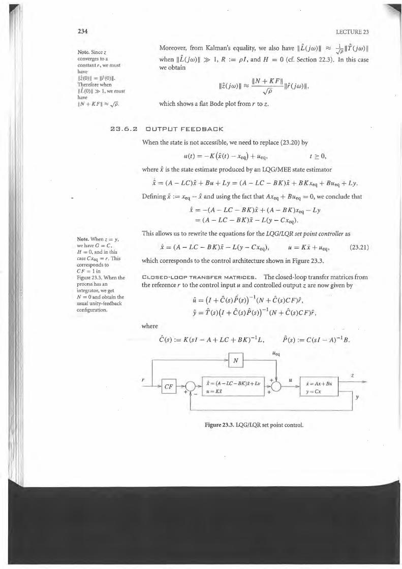
234

Note. Since z converges to a constant r, we must have lIi(O)1I = 11,0(0)11· Therefore when lIi(O)II» 1,wemust have

LECTURE 23

Moreover, from Kalman's equality, we also have IIL(jw)1I ~ )p1I1'(jw) II

when IIL(jw)1I » 1, R := pI, and H = ° (d. Section 22.3). In this case we obtain

IIz(jw)1I ~ liN + K Fllllr(jw)ll, .j15

liN + K FII ~ .JP. which shows a flat Bode plot from r to Z.

23.6.2 OUTPUT FEEDBACK

Note. When z = y, wehaveG = C, H = 0, and in this case CXeq = r. This corresponds to CF = 1 in Figure 23.3. When the process has an integrator, we get N = 0 and obtain the usual unity-feedback configuration.

When the state is not accessible, we need to replace (23.20) by

U(t) = -K(x(t) - Xeq) + ueq , t :::: 0,

where x is the state estimate produced by an LQG/MEE state estimator

; = (A - LC)x + Bu + Ly = (A - LC - BK)x + BKxeq + BUeq + Ly.

Defining x := Xeq - x and using the fact that AXeq + BUeq = 0, we conclude that

x = -(A - LC - BK)x + (A - BK)xeq - Ly

= (A - LC - BK)x - L(y - Cxeq ).

This allows us to rewrite the equations for the LQG/LQR set point controller as

x = (A - LC - BK)x - L(y - Cxeq ), U = Ki + ueq ,

which corresponds to the control architecture shown in Figure 23.3.

(23.21 )

CLOSED-LOOP TRANSFER MATRICES. The closed-loop transfer matrices from the reference r to the control input U and controlled output z are now given by

u = (I + C(s)p(s)r1(N + C(s)CF)r,

y = 1'(s)(I + C(s)p(s)r1(N + C(s)CF)r,

where

C(s) := K(sI ~ A + LC + BK)-l L, pes) := C(sI--' A)-J B.

z 1; G I , CF ~I x=(A_-LC-BK)i+LV ~I x=Ax+Bu I

+ l '~Kx +. y~Cx J ' Figure 23.3. LQG/LQR set point control.

OUTPUT FEEDBACK

When LTR succeeds, i.e., when

C(jw)P(jw) ~ iUw), Vw E [0, wmax ],

235

the main difference between these and the formulas seen before for state feedback is that the matrix N + K F multiplying by r has been replaced by the transfer matrix N + C(s)CF.

When N = 0, this generally leads to smaller transfer matrices when the loop gain is low, because we now have

u ~ C(s)CFr, y ~ Tcs)C(s)C Fr,

and C(s) falls at least at -20 dB/decade.

23.7 L4IR/L4IG WITH MATLAB®

Note. As discussed in Section 23.3, this LQG estimator is also an MEE estimator with cost (23.4), where Q = RN- 1 and R = QN- 1 (pay attention to the inverses and the exchange between Qs and Rs).

Note. See Example 23.1.

23.B

MATLAB® Hint 49. See MATLAB® Hints 46 (p. 235) and 47 (p.235).

MATLAB® Hint 46 (kalm.an). The command

[est,L,Pl=kalman(sys,QN,RN}

computes the optimal LQG estimator gain for the process

i = Ax + Bu + BBd, y = Cx +n,

where d(t) and net) are uncorrelated zero-mean Gaussian noise processes with co­variance matrices

E[d(t)d'(r») = o(t - r)QN, E[n(t)n'(r)] =o(t -r)RN.

The variable sys should be a state-space model created using

sys=ss(A, [B BBl,C,O).

This command returns the optimal estimator gain L, the solution P to the corre­sponding algebraic Riccati equation, and a state-space model es t for the estimator. The inputs to est are [u; y], and its outputs are [y; x].

For loop transfer rec<?very (LTR)"one should set

BB=B, QN= I, . RN = aI, a ~ O. o

MATLAB® Hint 47 (reg). The function reg (sys , K, L) computes a state-space model for a positive output feedback LQG/LQR controller for the process with state­space model sys with regulator gain K and estimator gain L. 0

LTR DESIGN EXAMPLE

Example 23.1 (Aircraft roll dynamics,continued). Figure 23.4(a) shows Bode plots of the open-loop gain for the state feedback LQR state feedback controller versus the open-loop gain for several output feedback LQG/LQR controllers obtained for the aircraft roll dynamics in Example 22.1. The LQR controller was designed using the controlled output z := [8 y e]', with y = 0.1 and p = 0.01 (see Example 22.1). For the LQG state estimators, we used the parameters for the loop transfer recovery theorem (Theorem 23.3): i3 = B, R = I, and Q = a for several values of a in the MEE cost (23.4) [or the corresponding LQG disturbance and noise (23.11)]. The matrix gain L, the LQG/LQR output feedback controller, and the corresponding Bode plot of the open-loop gain can be computed using the following sequence of MATLAB® commands:

236

23.9

Note. This result is less interesting than Theorem 23.2. because often (A, C) is not observable. just detectable. This can happen when we augmented the state of the system to construct a "good" controlled output z. but these augmented states are not observable through y.

l 00!r---~----------~----~---'

50

o -, ~. ,~ __

-50 ____ LOR open-loop gain T 'o~~ I

-100 -B- LQG/lQA open-loop gain, <1= 1('2 ~rtne.. ~... LOG/LQA open-loop gain. (1 = l OIS

-1 50 LOG/LOR Dpnn-kJop GRW1, n:o 1t1B

10' 10' 10' 10'

-BDr---------__ --------____ -.

-100

! -120

~ a -140

- 160

100 10' frequency [rad/s]

(a)

LECTURE 23

1~,-----~------~------~-----. ; \

I ,

I .~

1 I,'" ;.:'~'- __________________ _

o~ r"i! ~ r-------L~QR-o-p-en--I-oo-p-ga-'n-------oJ - - - LQGIlQR open-loop garn, 0'= l (Q - - LQGILQR open-loop gain, 0' = l e5

LQG/lQR open-loop gain, 0 = 1GB o o 0.5 15

lime

(b)

Figure 23.4. Bode plots of the open-loop gain and closed-loop step response for the LQR controllers in Example 23.1.

R=l; Q=sigma; Pka l=ss(A, [B BJ ,C,O);

% weight matrices % process for the kalman() % command

[est,Lj=kalman(Pkal,inv(R) ,inv(Q)); % compute LQG gain P=ss(A,B,C,O); % process for the reg()

% command Cs=-reg(P,K,L) ;

bode (Cs*P) ;

% LQG/LQR controller % (negative feedback) % bode plot of the % open-loop gain

We can see that, as a increases, the 'range of frequencies over which the open-loop gain of the output feedback LQG/LQR controller matches that of the state feedback LQR state feedback increases. Moreover, at high frequencies the output feedback controllers exhibit much faster (and better!) decays of the gain's magnitude. D

EXERCISES

23.1 (Solution to the dual ARE). Assume that the pair (-A, 8) is stabilizable and that the pair (A. C) is observabh~. Prove the following.

(a) There exists a symmetric positive-definite solution P to the ARE (23.5), for which - A - 8 R -181 P is a stability matrix.

(b) There exists a symmetric positive-definite solution S (23.7), for which A - LC is a stability matrix.

._ p-l to the dual ARE D

23.2. Show that ifthe pair (A, B) is controllable, then the pair

Y := SCI QC S + 8 R- 1 81•

OUTPUT FEEDBACK

is also controllable for Q and R symmetric and positive-definite.

Hint: Use the eigenvector test.

237

o 23.3 (Separation principle). Verify that the LQG/LQR controller (23.14) makes the closed-loop system asymptotically stable.

Hint: Write the state of the closed-loop system in terms of x and e := x-x. 0

23.4. Verify that a solution to (23.17) is given by (23.18).

Hint: Use direct substitution of the "candidate" solution into (23.17). o 23.5. Verify that the LQG/LQR set point controller (23.21) makes the closed-loop system asymptotically stable.

Hint: Write the state of the closed loop in terms of x - Xeq and e := x-x. 0

23.6 (Set point control with integrator). Show that for a single controlled output (l = 1), we can take ueq = 0 in (23.17) when the matrix A has an eigenvalue at the origin and this mode is observable through z. Note that in this case the process has an integrator. 0