Partial Differential Equations - MGNetdouglas/Classes/cs521/pde/pde2004.pdf · Partial Differential...

Partial Differential Equations

• Introduction, Adam Zornes• Discretizations and Iterative Solvers,

Chenfang Chen• Parallelization, Dr. Danny Thorne

What do You Stand For?

• A PDE is a Partial Differential Equation • This is an equation with derivatives of at

least two variables in it. • In general, partial differential equations are

much more difficult to solve analytically than are ordinary differential equations

What Does a PDE Look Like

• Let u be a function of x and y. There are several ways to write a PDE, e.g.,– ux + uy = 0– δu/δx + δu/δy = 0

The Baskin Robin’s esqCharacterization of PDE’s

• The order is determined by the maximum number of derivatives of any term.

• Linear/Nonlinear– A nonlinear PDE has the solution times a

partial derivative or a partial derivative raised to some power in it

• Elliptic/Parabolic/Hyperbolic

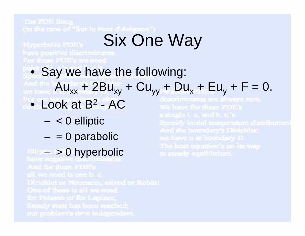
Six One Way

• Say we have the following:Auxx + 2Buxy + Cuyy + Dux + Euy + F = 0.

• Look at B2 - AC– < 0 elliptic – = 0 parabolic – > 0 hyperbolic

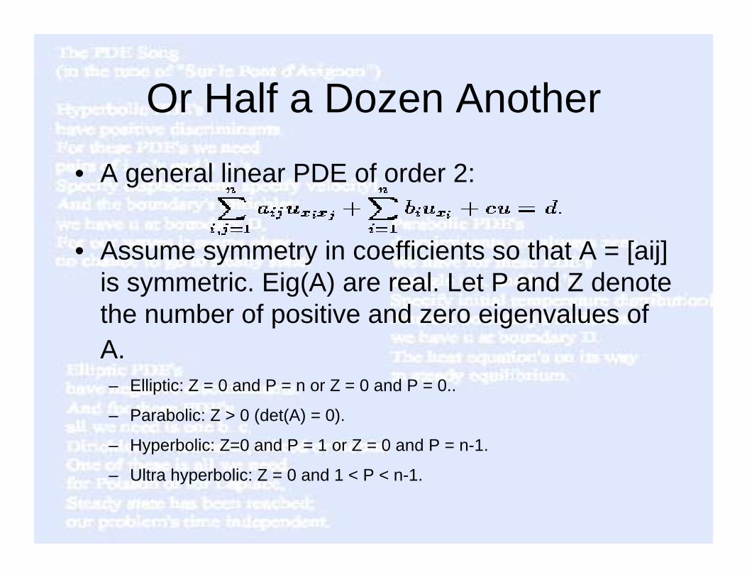
Or Half a Dozen Another

• A general linear PDE of order 2:

• Assume symmetry in coefficients so that A = [aij] is symmetric. Eig(A) are real. Let P and Z denote the number of positive and zero eigenvalues of A.– Elliptic: Z = 0 and P = n or Z = 0 and P = 0..

– Parabolic: Z > 0 (det(A) = 0).

– Hyperbolic: Z=0 and P = 1 or Z = 0 and P = n-1.

– Ultra hyperbolic: Z = 0 and 1 < P < n-1.

Elliptic, Not Just For Exercise Anymore

• Elliptic partial differential equations have applications in almost all areas of mathematics, from harmonic analysis to geometry to Lie theory, as well as numerous applications in physics.

• The basic example of an elliptic partial differential equation is Laplace’s Equation – uxx - uyy = 0

The Others

• The heat equation is the basic Hyperbolic – ut - uxx - uyy = 0

• The wave equations are the basic Parabolic– ut - ux - uy = 0– utt - uxx - uyy = 0

• Theoretically, all problems can be mapped to one of these

What Happens Where You Can’t Tell What Will Happen

• Types of boundary conditions– Dirichlet: specify the value of the function on a

surface – Neumann: specify the normal derivative of the

function on a surface– Robin: a linear combination of both

• Initial Conditions

Is It Worth the Effort?

• Basically, is it well-posed?– A solution to the problem exists. – The solution is unique. – The solution depends continuously on the

problem data.

• In practice, this usually involves correctly specifying the boundary conditions

Why Should You Stay Awake for the Remainder of the Talk?

• Enormous application to computational science, reaching into almost every nook and cranny of the field including, but not limited to: physics, chemistry, etc.

Example

• Laplace’s equation involves a steady state in systems of electric or magnetic fields in a vacuum or the steady flow of incompressible non-viscous fluids

• Poisson’s equation is a variation of Laplace when an outside force is applied to the system

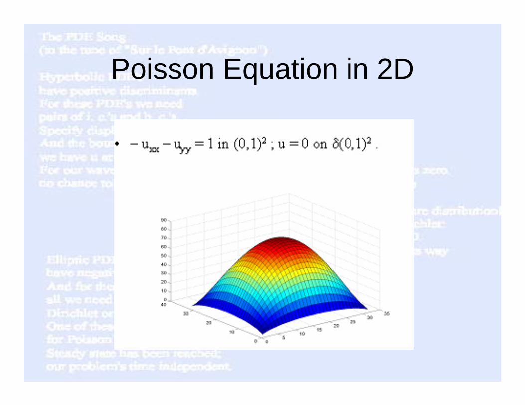
Poisson Equation in 2D

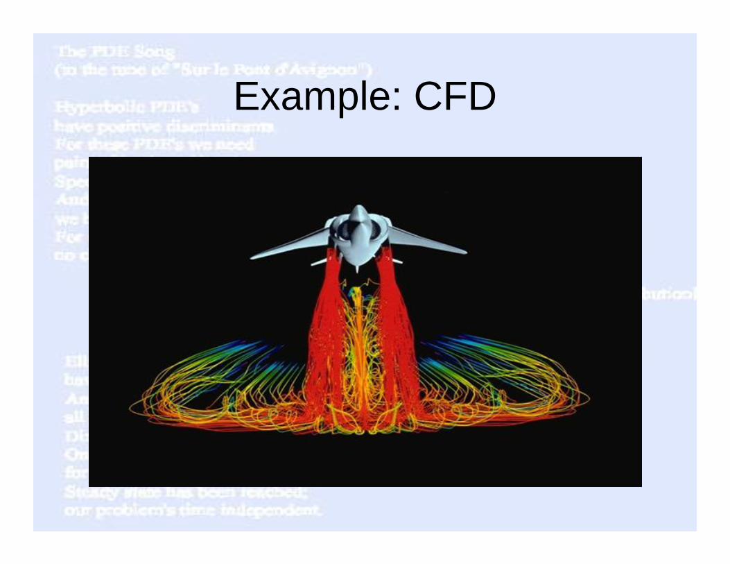
Example: CFD

Computational Fluid Dynamics

• CFD can be defined narrowly as confined to aerodynamic flow around vehicles but it can be generalized to include as well such areas as weather and climate simulation, flow of pollutants in the earth, and flow of liquids in oil fields (reservoir modelling).

• Involve Huge PDE’s• Computational Science only Realistic Solution

Links• http://www.npac.syr.edu/users/gcf/cps713overI94/• http://www.cse.uiuc.edu/~rjhartma/pdesong.html• http://www.maths.soton.ac.uk/teaching/units/ma274/nod

e2.html• http://www.npac.syr.edu/projects/csep/pde/pde.html• http://mathworld.wolfram.com/PartialDifferentialEquation.

html

DiscretizationDiscretization and and Iterative Method for Iterative Method for PDEsPDEs

ChunfangChunfang Chen Chen Danny ThorneDanny ThorneAdam Adam ZornesZornes

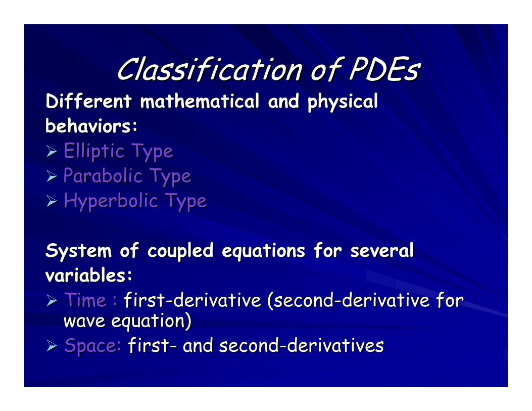
Classification of Classification of PDEsPDEsDifferent mathematical and physicalDifferent mathematical and physicalbehaviors:behaviors:

Elliptic TypeElliptic TypeParabolic TypeParabolic TypeHyperbolic TypeHyperbolic Type

System of coupled equations for several System of coupled equations for several variables:variables:

Time :Time : firstfirst--derivative (secondderivative (second--derivative for derivative for wave equation)wave equation)Space:Space: firstfirst-- and secondand second--derivativesderivatives

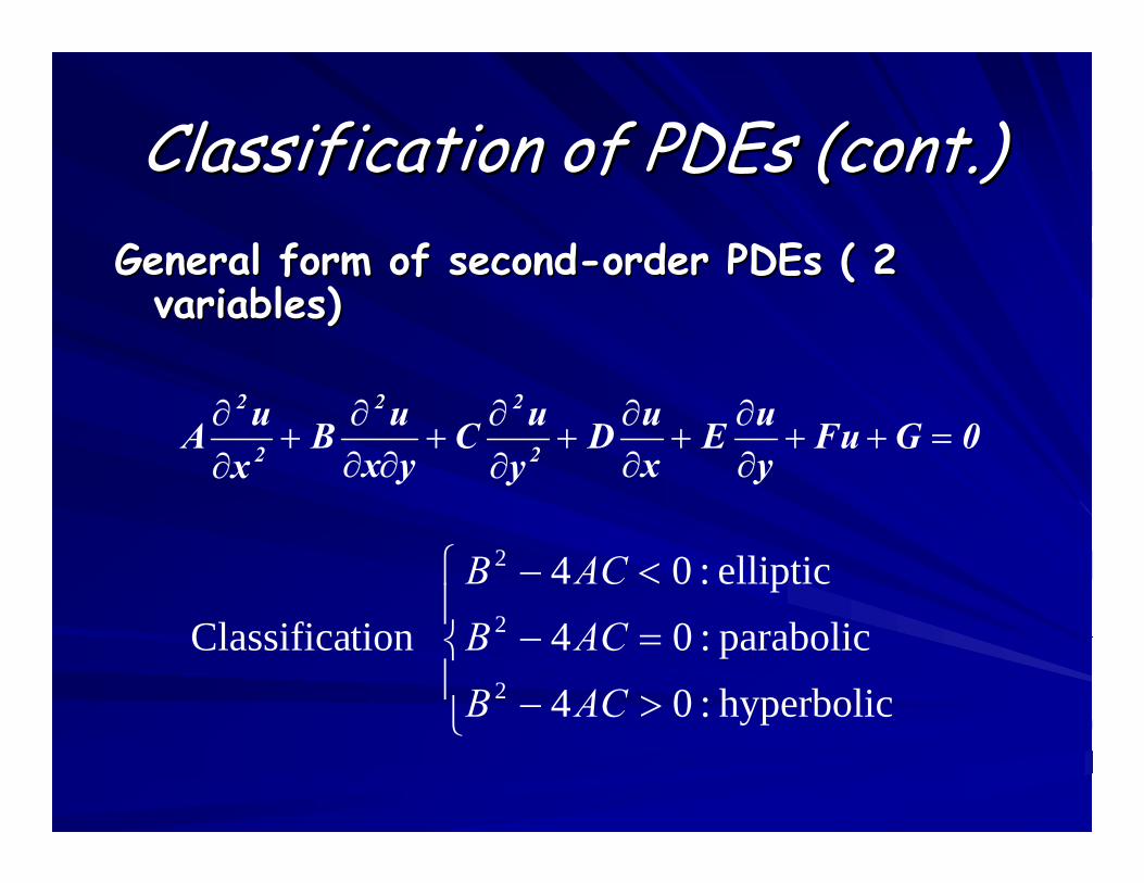
Classification of Classification of PDEsPDEs (cont.)(cont.)General form of secondGeneral form of second--order order PDEsPDEs ( 2 ( 2

variables)variables)

0GFuyuE

xuD

yuC

yxuB

xuA 2

22

2

2

=++∂∂

+∂∂

+∂∂

+∂∂

∂+

∂∂

⎪⎩

⎪⎨

⎧

>−

=−

<−

hyperbolic:04parabolic:04elliptic:04

tion Classifica2

2

2

ACBACBACB

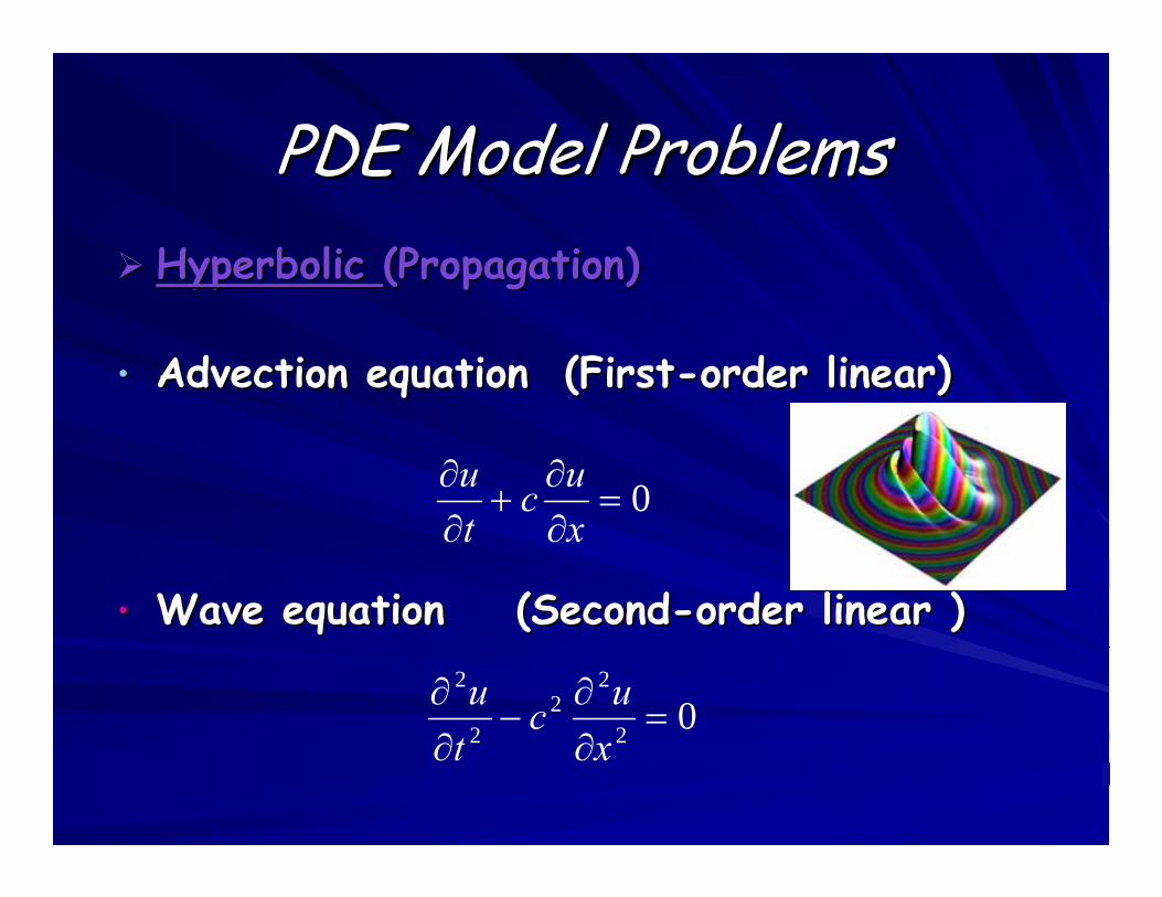
PDE Model ProblemsPDE Model ProblemsHyperbolic Hyperbolic (Propagation)(Propagation)

•• Advection equation (FirstAdvection equation (First--order linear)order linear)

•• Wave equation (SecondWave equation (Second--order linearorder linear ) )

0=∂∂

+∂∂

xuc

tu

02

22

2

2

=∂∂

−∂∂

xuc

tu

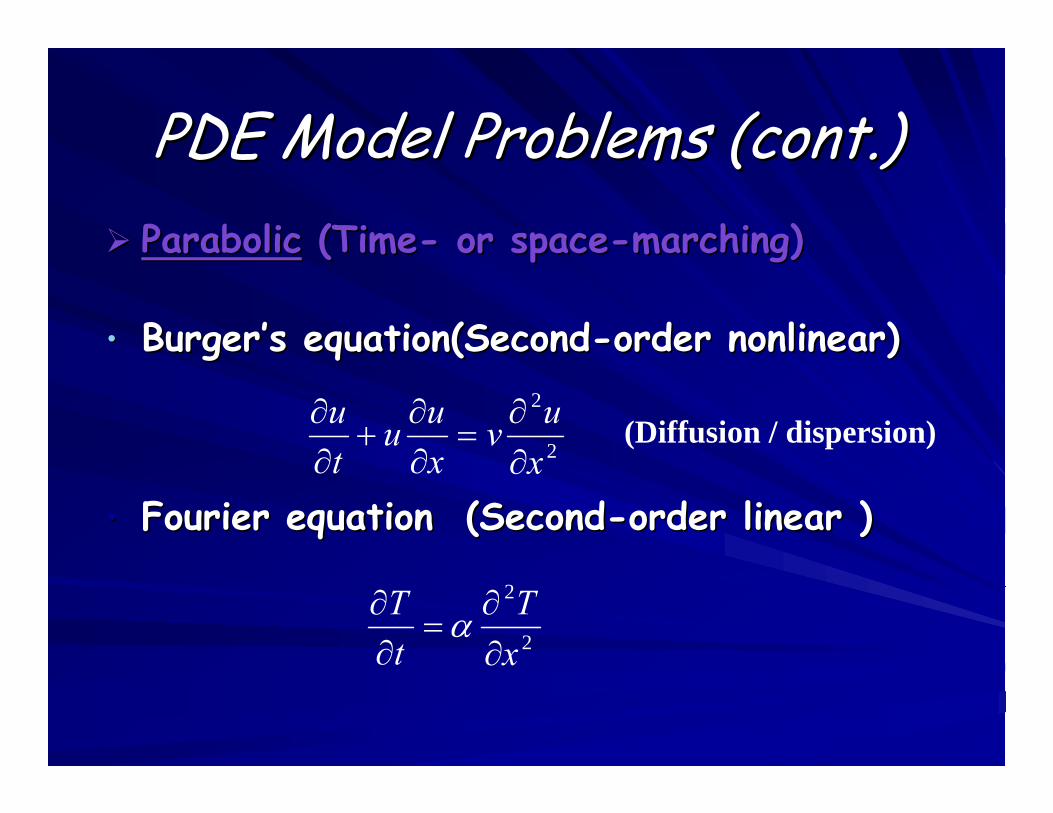
PDE Model Problems (cont.)PDE Model Problems (cont.)ParabolicParabolic (Time(Time-- or spaceor space--marching)marching)

•• BurgerBurger’’s equation(Seconds equation(Second--order nonlinear) order nonlinear)

•• Fourier equation (SecondFourier equation (Second--order linearorder linear ) )

(Diffusion / dispersion) xuν

xuu

tu

2

2

∂∂

=∂∂

+∂∂

2

2

xT

tT

∂∂

=∂∂ α

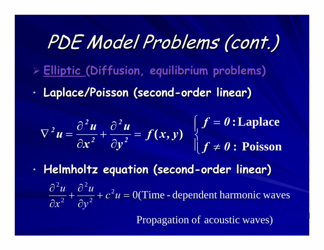
PDE Model Problems (cont.)PDE Model Problems (cont.)Elliptic Elliptic (Diffusion, equilibrium problems)(Diffusion, equilibrium problems)

•• Laplace/Poisson (secondLaplace/Poisson (second--order linear)order linear)

•• HelmholtzHelmholtz equation (secondequation (second--order linear)order linear)

) wavesacoustic ofn Propagatio

wavesharmonicdependent -Time(022

2

2

2

=+∂∂

+∂∂ uc

yu

xu

⎪⎩

⎪⎨⎧

≠

==

∂∂

+∂∂

=∇Poisson :

Laplace : ),(

0f

0fyxf

yu

xuu 2

2

2

22

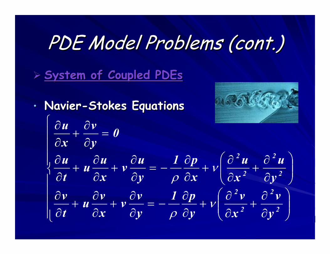
PDE Model Problems (cont.)PDE Model Problems (cont.)System of Coupled System of Coupled PDEsPDEs

•• NavierNavier--Stokes EquationsStokes Equations

⎪⎪⎪⎪

⎩

⎪⎪⎪⎪

⎨

⎧

⎟⎟⎠

⎞⎜⎜⎝

⎛∂∂

+∂∂

+∂∂

−=∂∂

+∂∂

+∂∂

⎟⎟⎠

⎞⎜⎜⎝

⎛∂∂

+∂∂

+∂∂

−=∂∂

+∂∂

+∂∂

=∂∂

+∂∂

2

2

2

2

2

2

2

2

yv

xv

yp1

yvv

xvu

tv

yu

xu

xp1

yuv

xuu

tu

0yv

xu

νρ

νρ

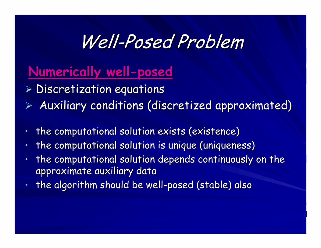
WellWell--Posed ProblemPosed ProblemNumerically wellNumerically well--posedposed

DiscretizationDiscretization equations equations Auxiliary conditions (Auxiliary conditions (discretizeddiscretized approximated)approximated)

•• the computational solution exists (existence)the computational solution exists (existence)•• the computational solution is unique (uniqueness)the computational solution is unique (uniqueness)•• the computational solution depends continuously on the the computational solution depends continuously on the

approximate auxiliary dataapproximate auxiliary data•• the algorithm should be wellthe algorithm should be well--posed (stable) alsoposed (stable) also

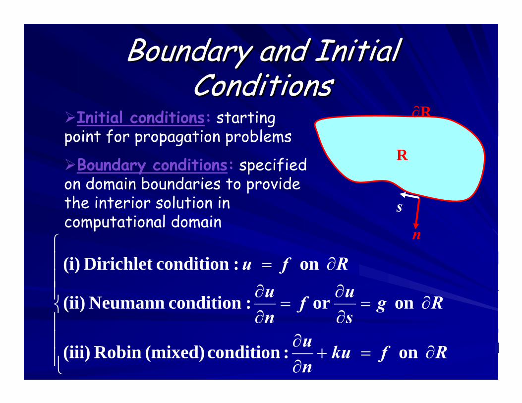
Boundary and InitialBoundary and InitialConditionsConditions

⎪⎪⎪

⎩

⎪⎪⎪

⎨

⎧

∂=+∂∂

∂=∂∂

=∂∂

∂=

on : condition (mixed) Robin (iii)

on or :condition Neumann (ii)

on :conditionDirichlet (i)

R fku nu

Rgsuf

nu

R fu

R

s

n

∂RInitial conditions: starting point for propagation problems

Boundary conditions: specified on domain boundaries to provide the interior solution in computational domain

Numerical MethodsNumerical MethodsComplex geometryComplex geometryComplex equations (nonlinear, coupled)Complex equations (nonlinear, coupled)Complex initial / boundary conditionsComplex initial / boundary conditions

No analytic solutionsNo analytic solutionsNumerical methods needed !!Numerical methods needed !!

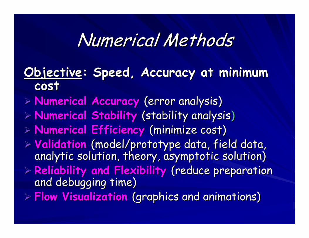
Numerical MethodsNumerical MethodsObjectiveObjective: Speed, Accuracy at minimum : Speed, Accuracy at minimum costcostNumerical AccuracyNumerical Accuracy (error analysis)(error analysis)Numerical StabilityNumerical Stability (stability analysis(stability analysis))Numerical Efficiency Numerical Efficiency (minimize cost)(minimize cost)Validation Validation (model/prototype data, field data, (model/prototype data, field data, analytic solution, theory, asymptotic solution)analytic solution, theory, asymptotic solution)Reliability and FlexibilityReliability and Flexibility (reduce preparation (reduce preparation and debugging time)and debugging time)Flow VisualizationFlow Visualization (graphics and animations)(graphics and animations)

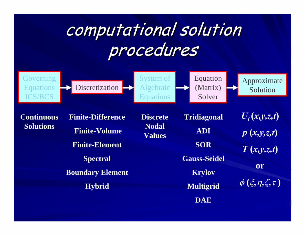
computational solution computational solution proceduresprocedures

Governing Equations ICS/BCS

DiscretizationSystem of Algebraic Equations

Equation (Matrix) Solver

ApproximateSolution

Continuous Solutions

Finite-Difference

Finite-Volume

Finite-Element

Spectral

Boundary Element

Hybrid

Discrete Nodal Values

Tridiagonal

ADI

SOR

Gauss-Seidel

Krylov

Multigrid

DAE

Ui (x,y,z,t)

p (x,y,z,t)

T (x,y,z,t)

or

φ (ξ,η,ζ,τ )

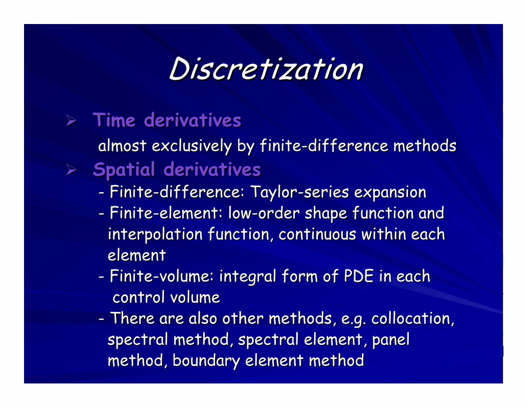
DiscretizationDiscretizationTime derivativesTime derivativesalmost exclusively by finitealmost exclusively by finite--difference methodsdifference methodsSpatial derivativesSpatial derivatives-- FiniteFinite--differencedifference: Taylor: Taylor--series expansionseries expansion-- FiniteFinite--elementelement: low: low--order shape function and order shape function and interpolation function, continuous within eachinterpolation function, continuous within eachelementelement

-- FiniteFinite--volumevolume: integral form of PDE in each: integral form of PDE in eachcontrol volumecontrol volume

-- There are also other methods, e.g. collocation,There are also other methods, e.g. collocation,spectral method, spectral element, panelspectral method, spectral element, panelmethod, boundary element methodmethod, boundary element method

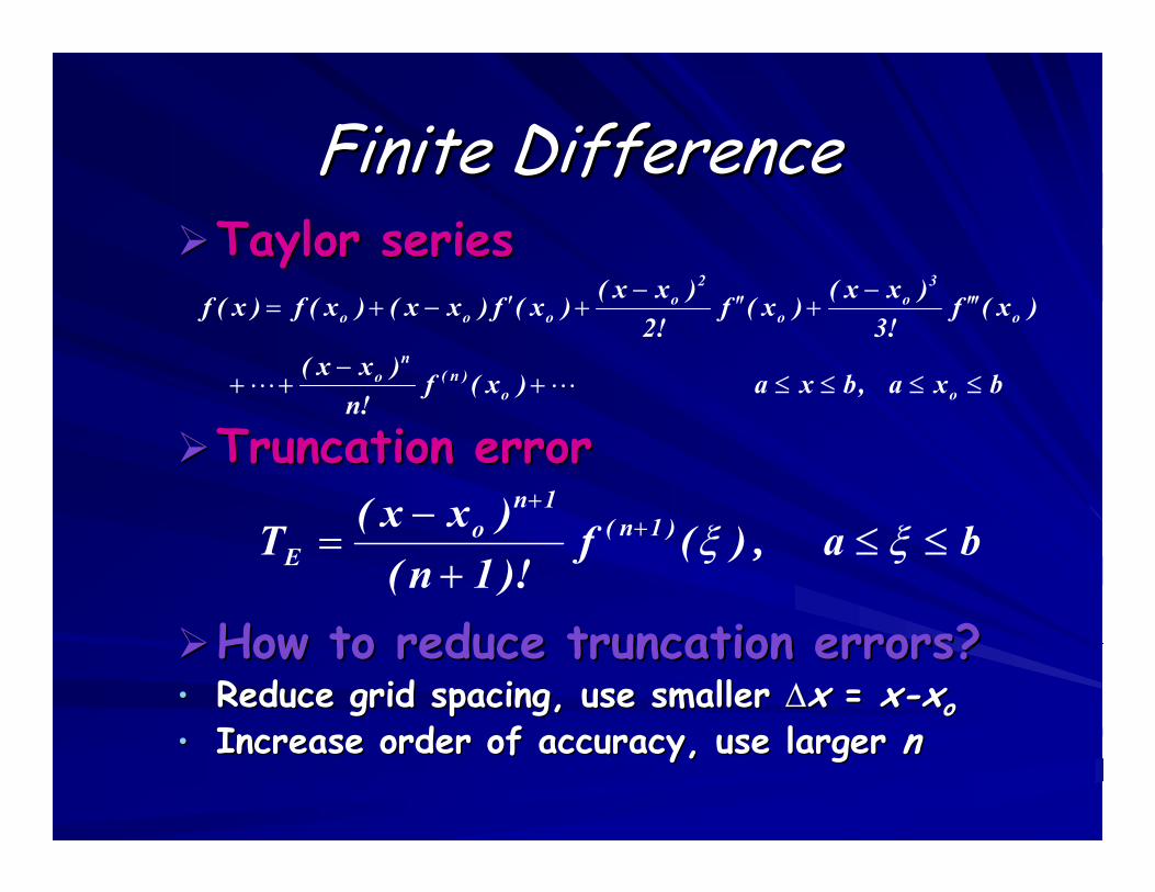
Finite DifferenceFinite DifferenceTaylor seriesTaylor series

Truncation errorTruncation error

How to reduce truncation errors?How to reduce truncation errors?•• Reduce grid spacing, use smaller Reduce grid spacing, use smaller ∆∆x x = = xx--xxoo•• Increase order of accuracy, use larger Increase order of accuracy, use larger nn

bxa,bxa)x(f!n

)xx(

)x(f!3

)xx()x(f

!2)xx(

)x(f)xx()x(f)x(f

oo)n(

no

o

3o

o

2o

ooo

≤≤≤≤+−

++

′′′−+′′−

+′−+=

ba)(f)!1n()xx(

T )1n(1n

oE ≤≤

+−

= ++

ξξ ,

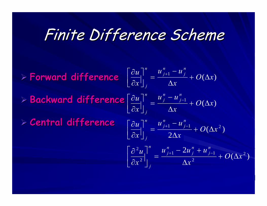
Finite Difference SchemeFinite Difference Scheme

Forward differenceForward difference

Backward differenceBackward difference

Central differenceCentral difference

)(2

)(2

)(

)(

22

112

2

211

1

1

xOx

uuuxu

xOxuu

xu

xOxuu

xu

xOx

uuxu

nj

nj

nj

n

j

nj

nj

n

j

nj

nj

n

j

nj

nj

n

j

∆+∆

+−=⎥

⎦

⎤⎢⎣

⎡∂∂

∆+∆

−=⎥⎦

⎤⎢⎣⎡∂∂

∆+∆

−=⎥⎦

⎤⎢⎣⎡∂∂

∆+∆

−=⎥⎦

⎤⎢⎣⎡∂∂

−+

−+

−

+

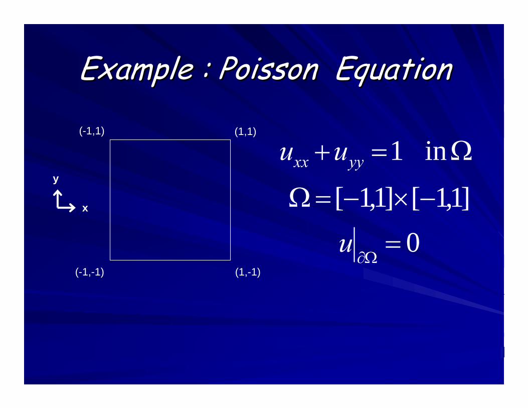
Example : Poisson EquationExample : Poisson Equation

(1,1)

(-1,-1) (1,-1)

(-1,1)

0]1,1[]1,1[

in 1

=

−×−=Ω

Ω=+

Ω∂u

uu yyxx

x

y

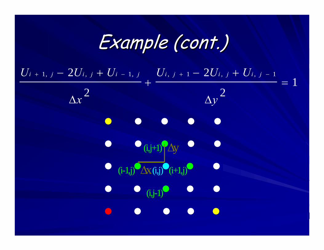
Example (cont.)Example (cont.)

12

2

2

2 1,,1,,1,,1=

∆

+−+

∆

+− −+−+

y

UUU

x

UUU jijijijijiji

• • • • • • • (i,j+1)•∆y • • • (i-1,j)•∆x (i,j)•(i+1,j)• • • • (i,j-1)• • • • • • • •

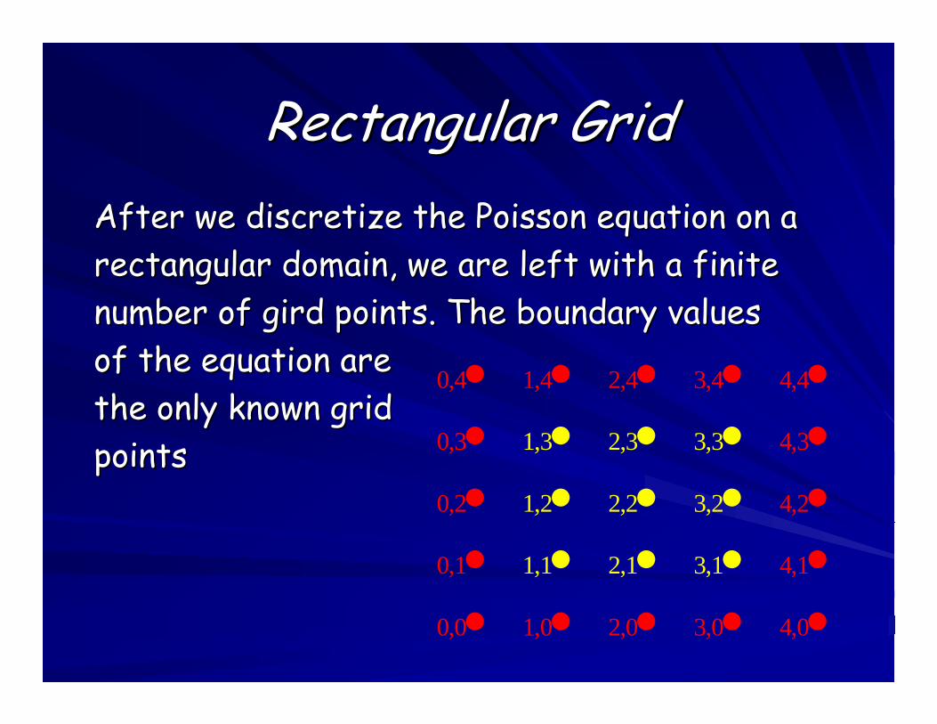
Rectangular GridRectangular GridAfter we After we discretizediscretize the Poisson equation on athe Poisson equation on arectangular domain, we are left with a finiterectangular domain, we are left with a finitenumber of gird points. The boundary valuesnumber of gird points. The boundary valuesof the equation are of the equation are the only known gridthe only known gridpoints points

0,4• 1,4• 2,4• 3,4• 4,4•0,3• 1,3• 2,3• 3,3• 4,3•0,2• 1,2• 2,2• 3,2• 4,2•0,1• 1,1• 2,1• 3,1• 4,1•0,0• 1,0• 2,0• 3,0• 4,0•

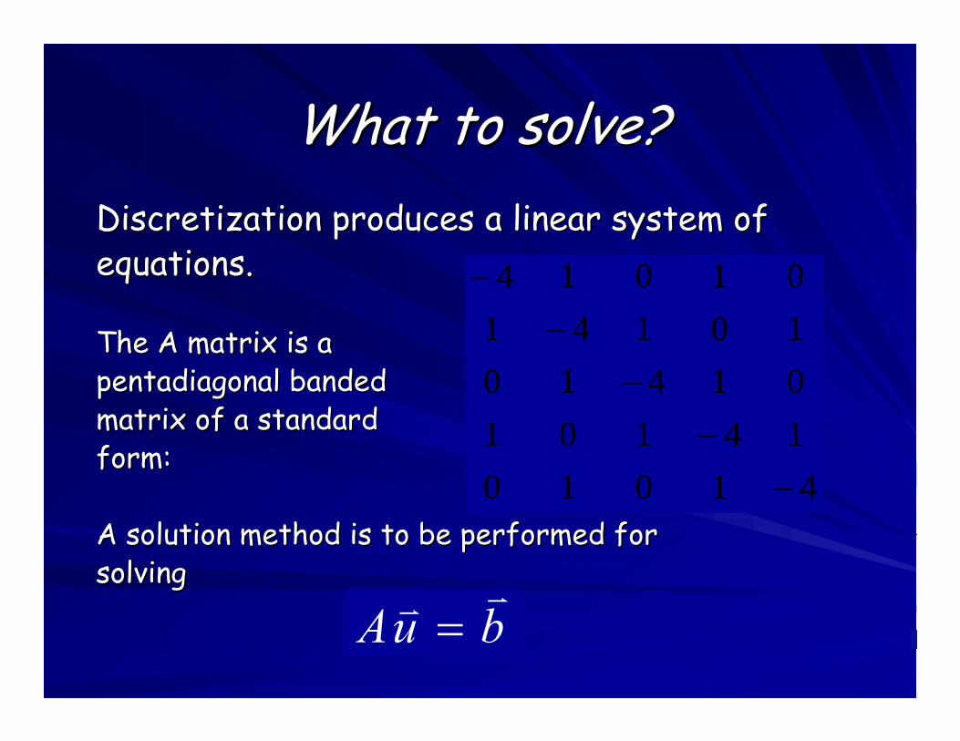
What to solve?What to solve?DiscretizationDiscretization produces a linear system ofproduces a linear system ofequations. equations.

The A matrix is aThe A matrix is apentadiagonalpentadiagonal bandedbandedmatrix of a standardmatrix of a standardform:form:

A solution method is to be performed forA solution method is to be performed forsolvingsolving

4101014101014101014101014

−−

−−

−

buA =

Matrix StorageMatrix Storage

We could try and take advantage of the We could try and take advantage of the banded nature of the system, but a banded nature of the system, but a more general solution is the adoption of more general solution is the adoption of a sparse matrix storage strategy.a sparse matrix storage strategy.

Limitations of Finite Limitations of Finite DifferencesDifferences

Unfortunately, it is not easy to use Unfortunately, it is not easy to use finite differences in complex finite differences in complex geometries.geometries.While it is possible to formulate While it is possible to formulate curvilinear finite difference methods, curvilinear finite difference methods, the resulting equations are usually the resulting equations are usually pretty nasty.pretty nasty.

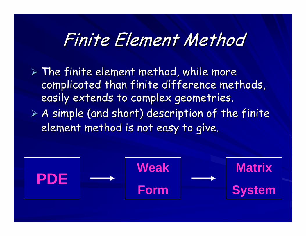
Finite Element MethodFinite Element MethodThe finite element method, while more The finite element method, while more complicated than finite difference methods, complicated than finite difference methods, easily extends to complex geometries.easily extends to complex geometries.A simple (and short) description of the finite A simple (and short) description of the finite element method is not easy to give.element method is not easy to give.

PDEWeak

Form

Matrix

System

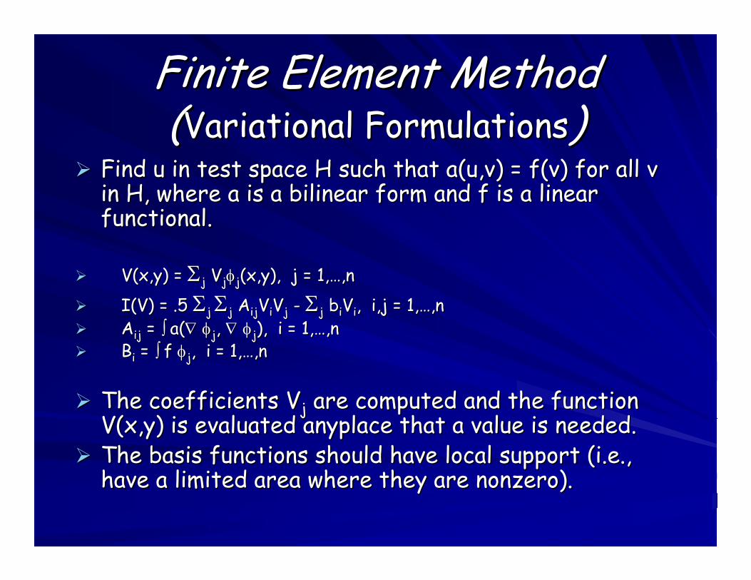
Finite Element Method Finite Element Method ((VariationalVariational FormulationsFormulations))

Find u in test space H such that a(u,v) = f(v) for all v Find u in test space H such that a(u,v) = f(v) for all v in H, where a is a bilinear form and f is a linear in H, where a is a bilinear form and f is a linear functional.functional.

V(x,y) = V(x,y) = ΣΣjj VVjjφφjj(x,y), j = 1,(x,y), j = 1,……,n,n

I(V) = .5 I(V) = .5 ΣΣj j ΣΣjj AAijijVViiVVjj -- ΣΣjj bbiiVVii, i,j = 1,, i,j = 1,……,n,nAAijij = = ∫∫ a(a(∇∇ φφjj, , ∇∇ φφjj), i = 1,), i = 1,……,n,nBBii = = ∫∫ f f φφjj, i = 1,, i = 1,……,n,n

The coefficients VThe coefficients Vjj are computed and the function are computed and the function V(x,y) is evaluated anyplace that a value is needed.V(x,y) is evaluated anyplace that a value is needed.The basis functions should have local support (i.e., The basis functions should have local support (i.e., have a limited area where they are nonzero).have a limited area where they are nonzero).

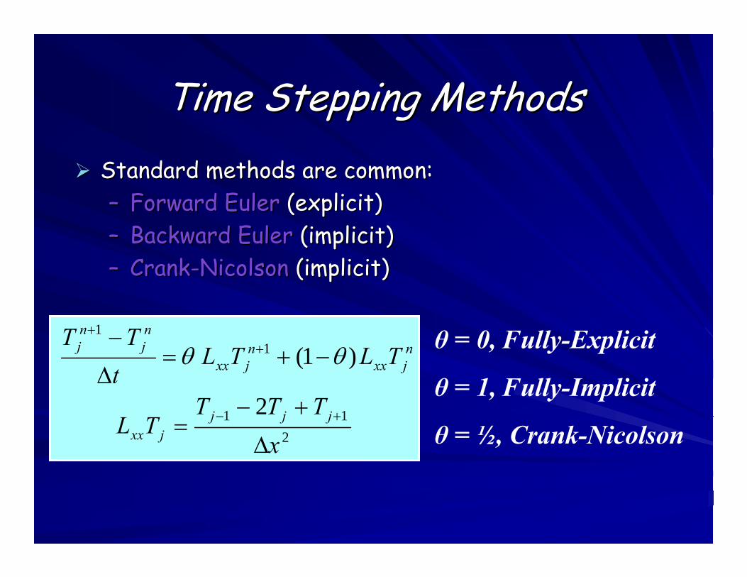
Time Stepping MethodsTime Stepping MethodsStandard methods are common:Standard methods are common:–– Forward EulerForward Euler (explicit)(explicit)–– Backward EulerBackward Euler (implicit)(implicit)–– CrankCrank--NicolsonNicolson (implicit)(implicit)

211

1

1

2

)1(

xTTT

TL

TLTLt

TT

jjjjxx

njxx

njxx

nj

nj

∆

+−=

−+=∆

−

+−

++

θθθ = 0, Fully-Explicit

θ = 1, Fully-Implicit

θ = ½, Crank-Nicolson

Time Stepping Methods (cont.)Time Stepping Methods (cont.)Variable length time steppingVariable length time stepping–– Most common in Method of Lines (Most common in Method of Lines (MOLMOL) codes or ) codes or

Differential Algebraic Equation (Differential Algebraic Equation (DAEDAE) solvers) solvers

Solving the SystemSolving the SystemThe system may be solved using simple The system may be solved using simple iterative methods iterative methods -- JacobiJacobi, Gauss, Gauss--Seidel, Seidel, SOR, etc.SOR, etc.

•• Some advantages:Some advantages:-- No explicit storage of the matrix is requiredNo explicit storage of the matrix is required-- The methods are fairly robust and reliableThe methods are fairly robust and reliable

•• Some disadvantagesSome disadvantages-- Really slow (GaussReally slow (Gauss--Seidel)Seidel)-- Really slow (Really slow (JacobiJacobi))

Solving the SystemSolving the SystemAdvanced iterative methods (CG, GMRES)Advanced iterative methods (CG, GMRES)

CG is a much more powerful way to solve the CG is a much more powerful way to solve the problem.problem.

•• Some advantages:Some advantages:–– Easy to program (compared to other advanced Easy to program (compared to other advanced

methods)methods)–– Fast (theoretical convergence in N steps for an N Fast (theoretical convergence in N steps for an N

by N system)by N system)•• Some disadvantages:Some disadvantages:

–– Explicit representation of the matrix is probably Explicit representation of the matrix is probably necessarynecessary

–– Applies only to SPD matrices Applies only to SPD matrices

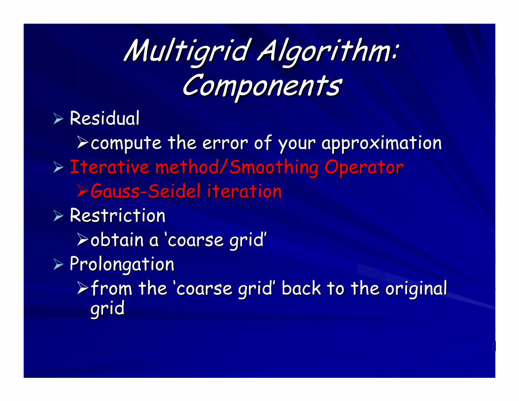
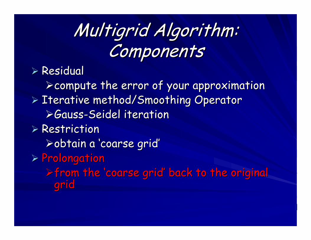
MultigridMultigrid Algorithm: Algorithm: ComponentsComponents

ResidualResidualcompute the error of the approximationcompute the error of the approximation

Iterative method/Smoothing OperatorIterative method/Smoothing OperatorGaussGauss--Seidel iterationSeidel iteration

RestrictionRestrictionobtain a obtain a ‘‘coarse gridcoarse grid’’

ProlongationProlongationfrom the from the ‘‘coarse gridcoarse grid’’ back to the back to the original gridoriginal grid

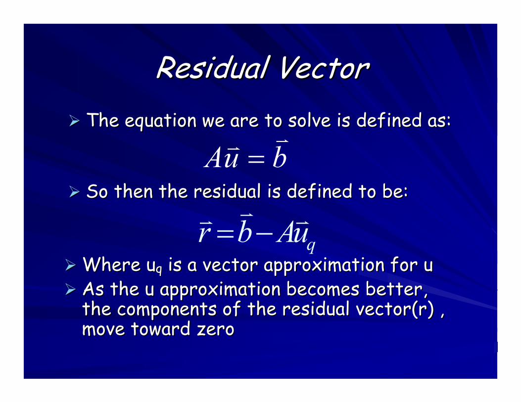
Residual VectorResidual VectorThe equation we are to solve is defined as:The equation we are to solve is defined as:

So then the residual is defined to be:So then the residual is defined to be:

Where Where uuqq is a vector approximation for uis a vector approximation for uAs the u approximation becomes better, As the u approximation becomes better, the components of the residual vector(r) , the components of the residual vector(r) , move toward zeromove toward zero

buA =

quAbr −=


ResidualResidualcompute the error of your approximationcompute the error of your approximation



ProlongationProlongationfrom the from the ‘‘coarse gridcoarse grid’’ back to the original back to the original gridgrid






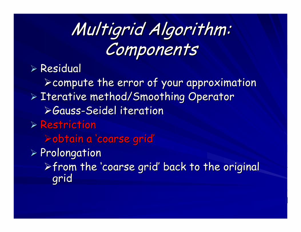
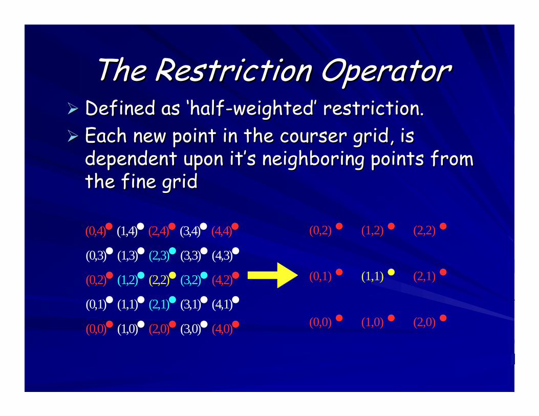
The Restriction OperatorThe Restriction OperatorDefined as Defined as ‘‘halfhalf--weightedweighted’’ restriction.restriction.Each new point in the courser grid, is Each new point in the courser grid, is dependent upon itdependent upon it’’s neighboring points from s neighboring points from the fine gridthe fine grid

(0,4)• (1,4)• (2,4)• (3,4)• (4,4)• (0,3)• (1,3)• (2,3)• (3,3)• (4,3)• (0,2)• (1,2)• (2,2)• (3,2)• (4,2)• (0,1)• (1,1)• (2,1)• (3,1)• (4,1)• (0,0)• (1,0)• (2,0)• (3,0)• (4,0)•

(0,2) • (1,2) • (2,2) •

(0,1) • (1,1) • (2,1) •

(0,0) • (1,0) • (2,0) •






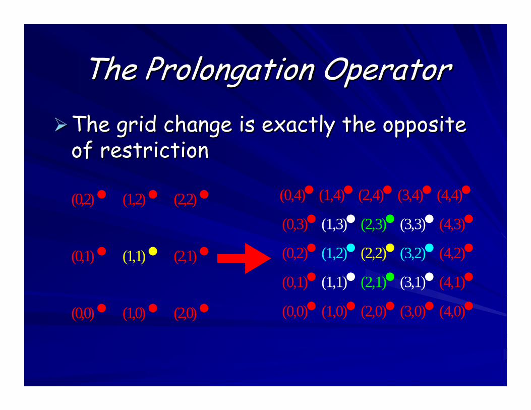
The Prolongation OperatorThe Prolongation OperatorThe grid change is exactly the opposite The grid change is exactly the opposite of restrictionof restriction

(0,2) • (1,2) • (2,2) •

(0,1) • (1,1) • (2,1) •

(0,0) • (1,0) • (2,0) •

(0,4)• (1,4)• (2,4)• (3,4)• (4,4)• (0,3)• (1,3)• (2,3)• (3,3)• (4,3)• (0,2)• (1,2)• (2,2)• (3,2)• (4,2)• (0,1)• (1,1)• (2,1)• (3,1)• (4,1)• (0,0)• (1,0)• (2,0)• (3,0)• (4,0)•

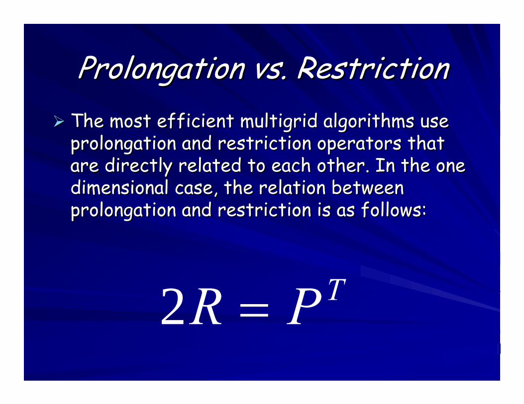
Prolongation vs. RestrictionProlongation vs. RestrictionThe most efficient multigrid algorithms use The most efficient multigrid algorithms use prolongation and restriction operators that prolongation and restriction operators that are directly related to each other. In the one are directly related to each other. In the one dimensional case, the relation between dimensional case, the relation between prolongation and restriction is as follows:prolongation and restriction is as follows:

TPR =2

Full Full MultigridMultigrid AlgorithmAlgorithm

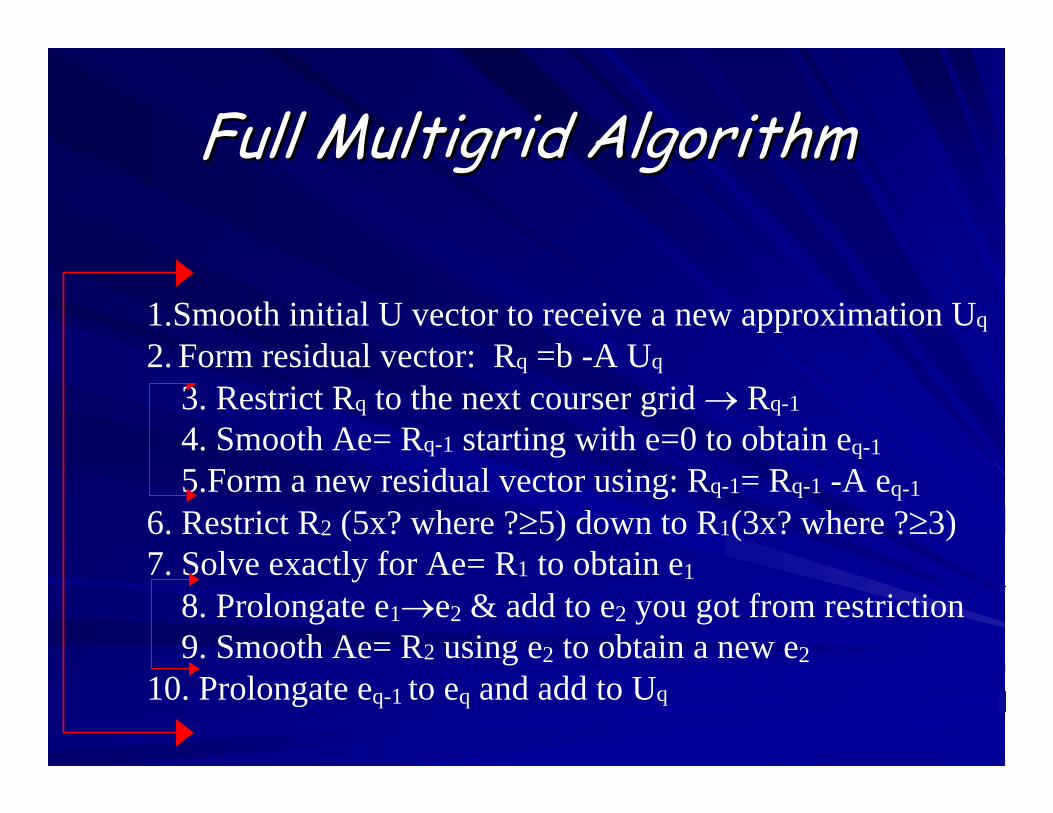
1.Smooth initial U vector to receive a new approximation Uq

2. Form residual vector: Rq =b -A Uq

3. Restrict Rq to the next courser grid → Rq-1

4. Smooth Ae= Rq-1 starting with e=0 to obtain eq-1

5.Form a new residual vector using: Rq-1= Rq-1 -A eq-1

6. Restrict R2 (5x? where ?≥5) down to R1(3x? where ?≥3)7. Solve exactly for Ae= R1 to obtain e1

8. Prolongate e1→e2 & add to e2 you got from restriction9. Smooth Ae= R2 using e2 to obtain a new e2

10. Prolongate eq-1 to eq and add to Uq

ReferenceReferencehttp://csep1.phy.ornl.gov/CSEP/PDE/PDE.htmhttp://csep1.phy.ornl.gov/CSEP/PDE/PDE.htmllwww.www.mgnetmgnet.org/ .org/ www.www.ceprofsceprofs..tamutamu..eduedu//hchenhchen/ / www.cs.cmu.edu/~ph/859B/www/notes/multigwww.cs.cmu.edu/~ph/859B/www/notes/multigrid.pdf rid.pdf www.cs.ucsd.edu/users/carter/260 www.cs.ucsd.edu/users/carter/260 www.cs.uh.edu/~chapman/teachpubs/slides04www.cs.uh.edu/~chapman/teachpubs/slides04--methods.ppt methods.ppt http://www.ccs.uky.edu/~douglas/Classes/cs5http://www.ccs.uky.edu/~douglas/Classes/cs52121--s01/index.htmls01/index.html

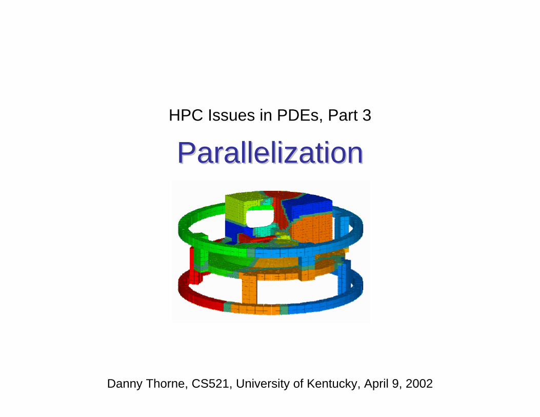
ParallelizationParallelizationHPC Issues in PDEs, Part 3

Danny Thorne, CS521, University of Kentucky, April 9, 2002

Parallel ComputationParallel Computation• Serious calculations today are mostly done on a parallel

computer.

• The domain is partitioned into subdomains that may or may not overlap slightly.

• Goal is to calculate as many things in parallel as possible even if some things have to be calculated on several processors in order to avoid communication.

• ”Communication is the Darth Vader of parallel computing.”

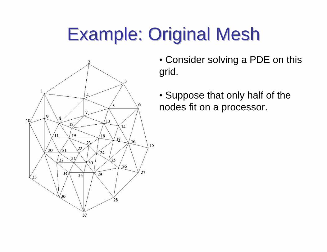
Example: Original MeshExample: Original Mesh• Consider solving a PDE on this grid.

• Suppose that only half of the nodes fit on a processor.

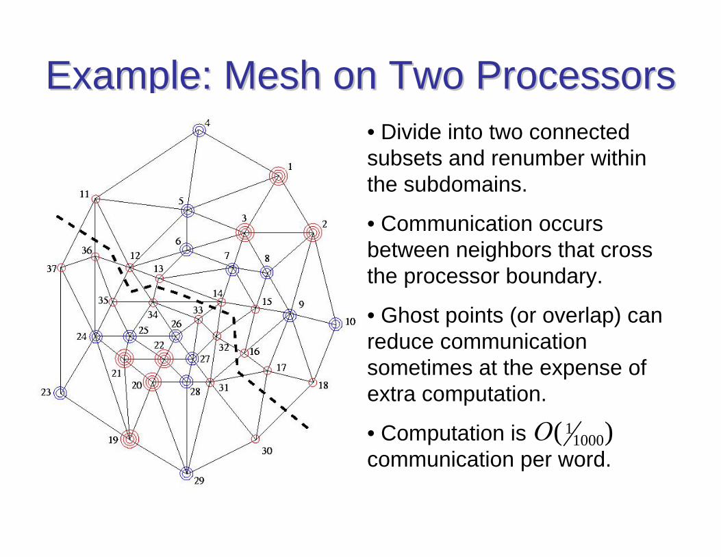
Example: Mesh on Two ProcessorsExample: Mesh on Two Processors• Divide into two connected subsets and renumber within the subdomains.

• Communication occurs between neighbors that cross the processor boundary.

• Ghost points (or overlap) can reduce communication sometimes at the expense of extra computation.

• Computation is communication per word.

)( 10001O

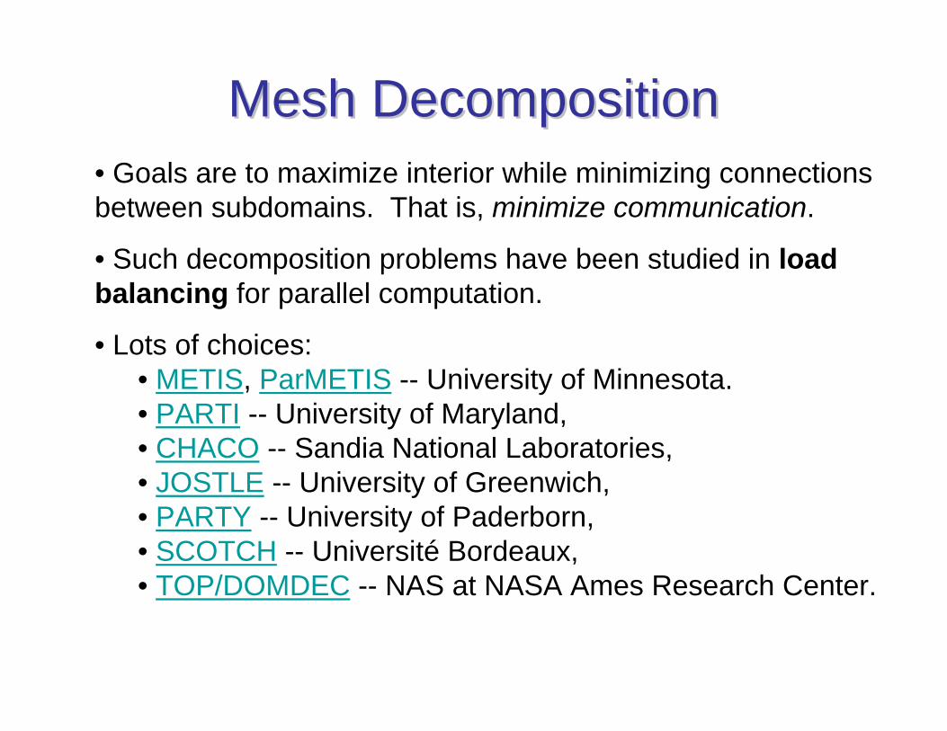
Mesh DecompositionMesh Decomposition• Goals are to maximize interior while minimizing connections between subdomains. That is, minimize communication.

• Such decomposition problems have been studied in load balancing for parallel computation.

• Lots of choices:• METIS, ParMETIS -- University of Minnesota.• PARTI -- University of Maryland,• CHACO -- Sandia National Laboratories,• JOSTLE -- University of Greenwich,• PARTY -- University of Paderborn,• SCOTCH -- Université Bordeaux,• TOP/DOMDEC -- NAS at NASA Ames Research Center.

Graph Partitioning Software• CHACO Bruce Hendrickson and Robert Leland Sandia

National Laboratories.• JOSTLE Chris Walshaw University of Greenwich. • METIS George Karypis and Vipin Kumar University of

Minnesota. • ParMETIS George Karypis, Kirk Schloegel, and Vipin Kumar

University of Minnesota. • PARTY Robert Preis and Ralf Diekmann University of

Paderborn • SCOTCH François Pellegrini Université Bordeaux • TOP/DOMDEC Horst D. Simon and Charbel Farhat NAS at

NASA Ames Research Center

http://www.erc.msstate.edu/~bilderba/research/other_sites.html

Mesh DecompositionMesh Decomposition• Quality of mesh decomposition has a highly significant effect on performance.

• Arriving at a “good” decomposition is a complex task.

• “Good” may be problem/architecture dependent.

• A wide variety of well-established methods exist.

• Several packages/libraries provide implementations of many of these methods.

• Major practical difficulty is differences in file formats.

http://www.epcc.ed.ac.uk/epcc-tec/documents/meshdecomp-slides/MeshDecomp-11.html

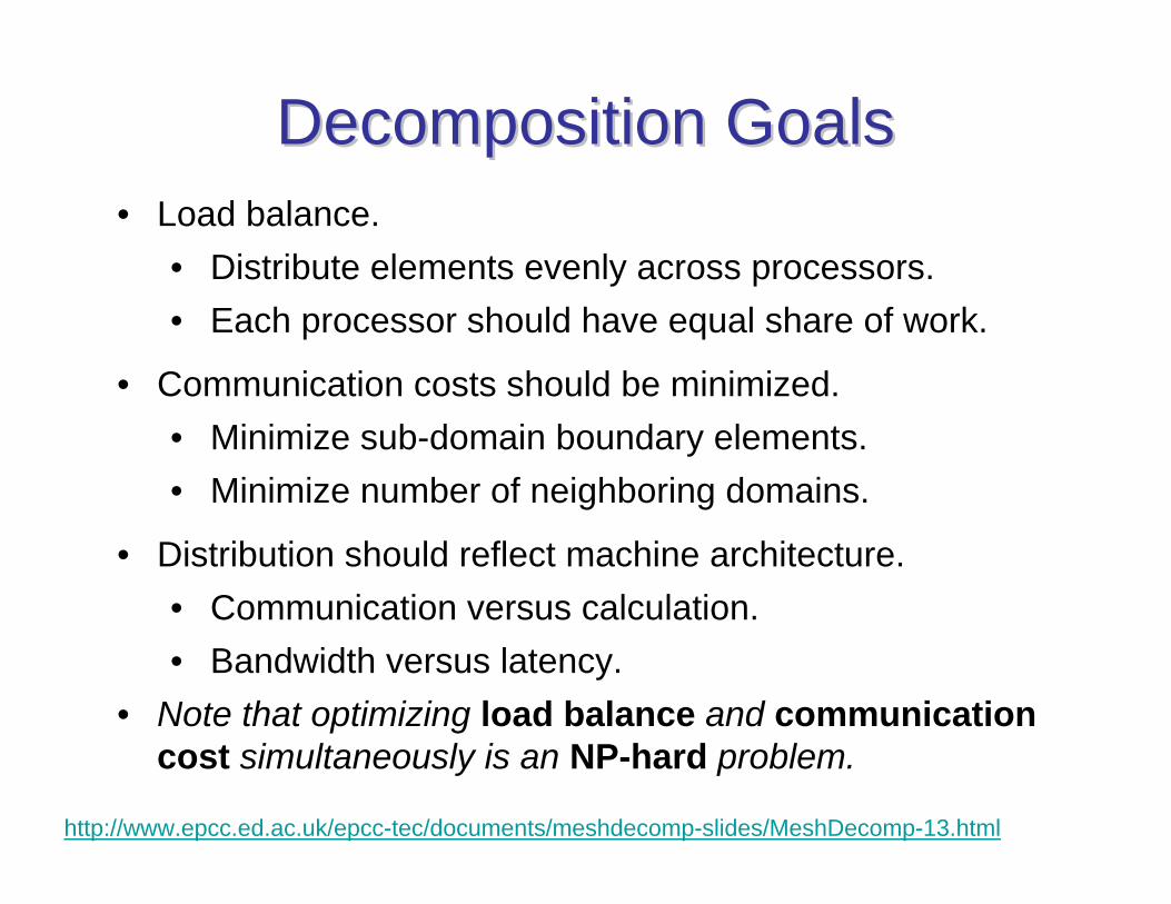
Decomposition GoalsDecomposition Goals• Load balance.

• Distribute elements evenly across processors.• Each processor should have equal share of work.

• Communication costs should be minimized. • Minimize sub-domain boundary elements.• Minimize number of neighboring domains.

• Distribution should reflect machine architecture.• Communication versus calculation.• Bandwidth versus latency.

• Note that optimizing load balance and communication cost simultaneously is an NP-hard problem.


Static Mesh versus Dynamic MeshStatic Mesh versus Dynamic Mesh• Static mesh

• Decomposition need only be carried out once.

• Static decomposition may therefore be carried out as a preprocessing step, often done in serial.

• Dynamic mesh

• Decomposition must be adapted as underlying mesh changes.

• Dynamic decomposition therefore becomes part of the calculation itself and cannot be carried out solely as a pre-processing step.


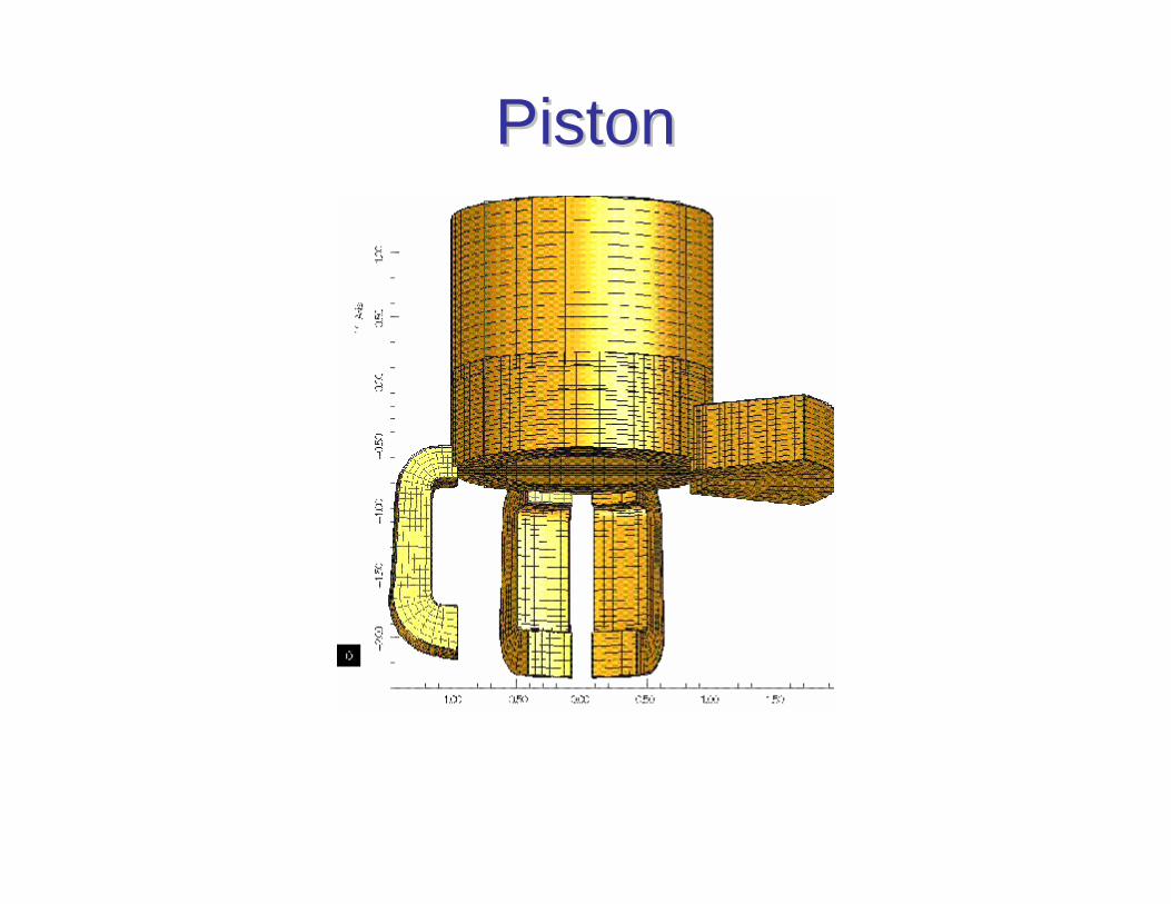
PistonPiston

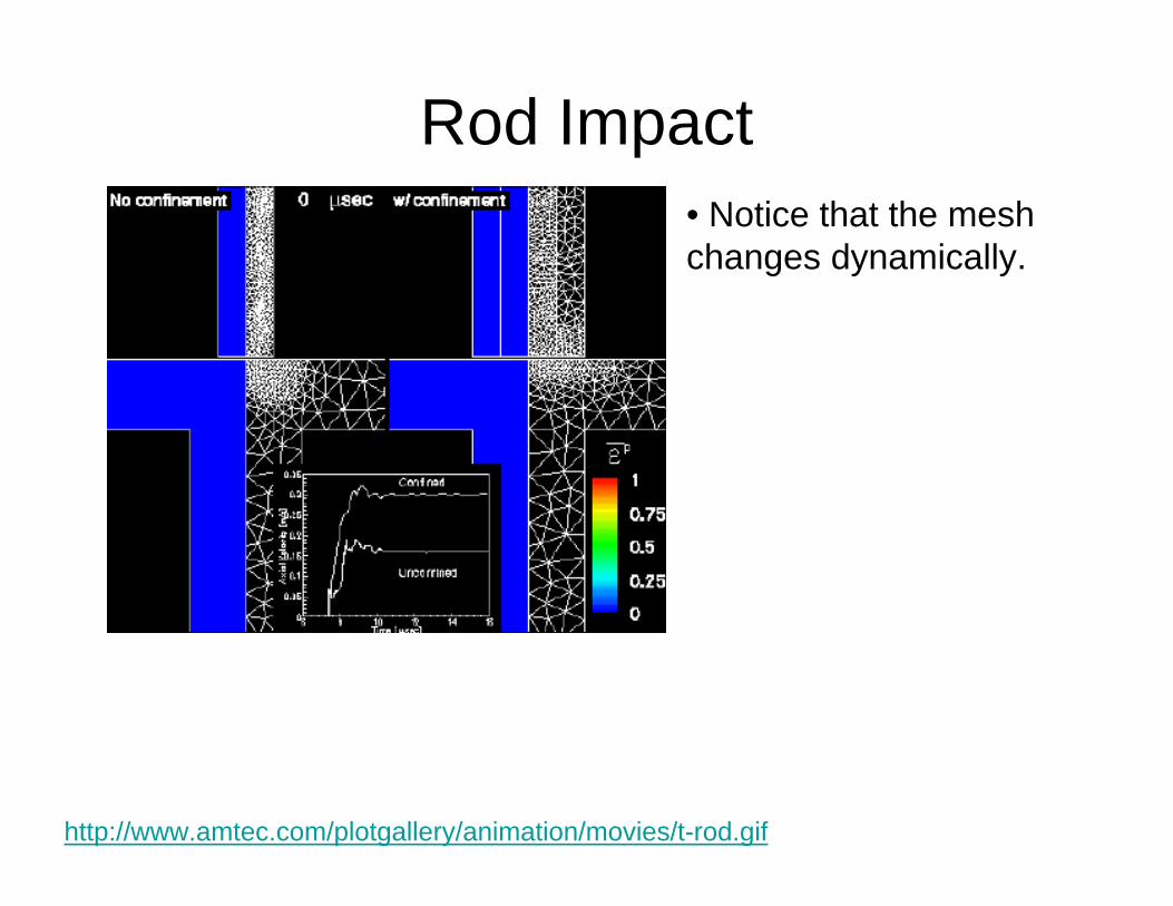
Rod Impact• Notice that the mesh changes dynamically.

http://www.amtec.com/plotgallery/animation/movies/t-rod.gif

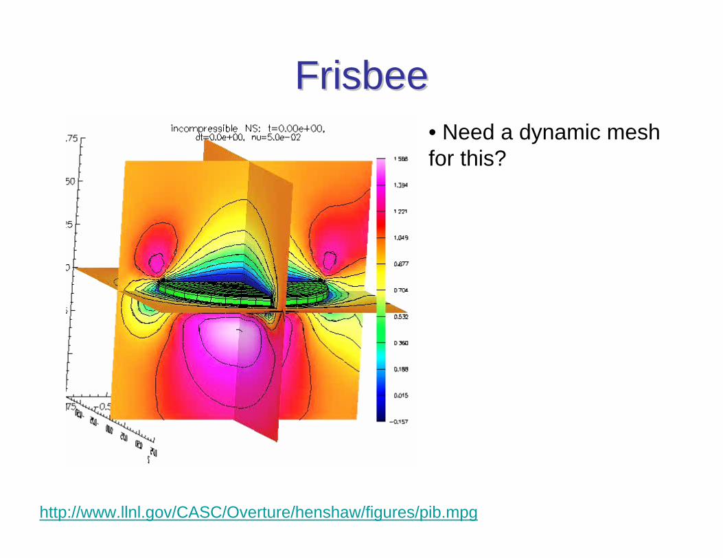
FrisbeeFrisbee

http://www.llnl.gov/CASC/Overture/henshaw/figures/pib.mpg

• Need a dynamic mesh for this?

Dynamic DecompositionDynamic Decomposition• To redistribute a mesh

• A new decomposition must be found and required changes made (shuffling of data between processors).

• The time taken may outweigh the benefit gained so an assessment of whether it is worthwhile is needed.

• The decomposition must run in parallel and be fast.

• Take into account the old decomposition.

• Make minimal changes.


Dual GraphsDual Graphs• To make a decomposition we need

• A representation of the basic entities being distributed (e.g. the elements, in the case of a FE mesh),• An idea of how communication takes place between them.

• A dual graph, based on the mesh, fills this role.• Vertices in the graph represent the entities (elements).• Edges in the graph represent communication.

• Graph depends on how data is transferred.• For finite elements it could be via nodes, edges or faces.• So a single mesh can have more than one dual graph.

• Edges (communications) or vertices (calculations) may be weighted.


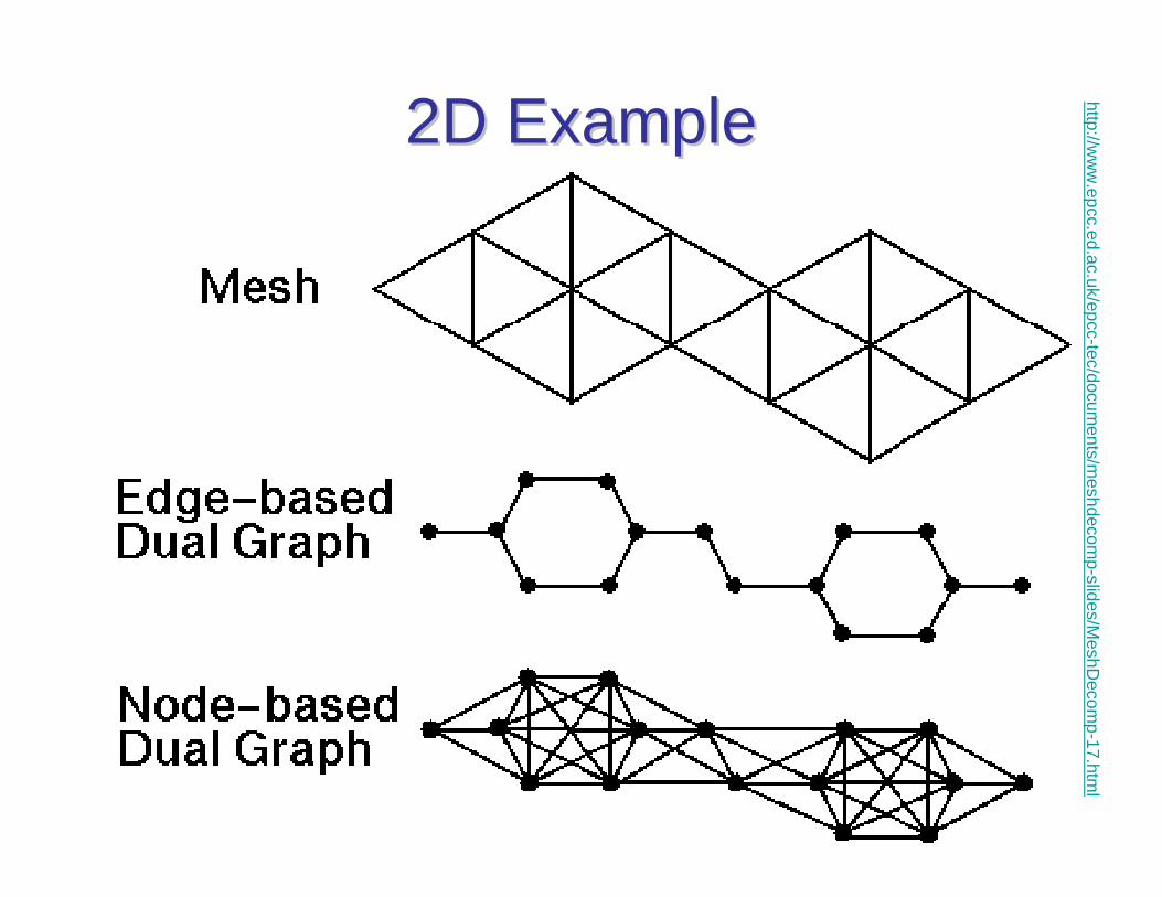
2D Example2D Example http://ww

w.epcc.ed.ac.uk/epcc-tec/docum

ents/meshdecom

p-slides/MeshD

ecomp-17.htm

l

Graph PartitioningGraph Partitioning• This problem occurs in several applications.

• VLSI circuit layout design,• Efficient orderings for parallel sparse matrix factorization,• Mesh decomposition.

• This problem has been extensively studied.• A large body of literature already exists.• Much work is still being produced in the field.


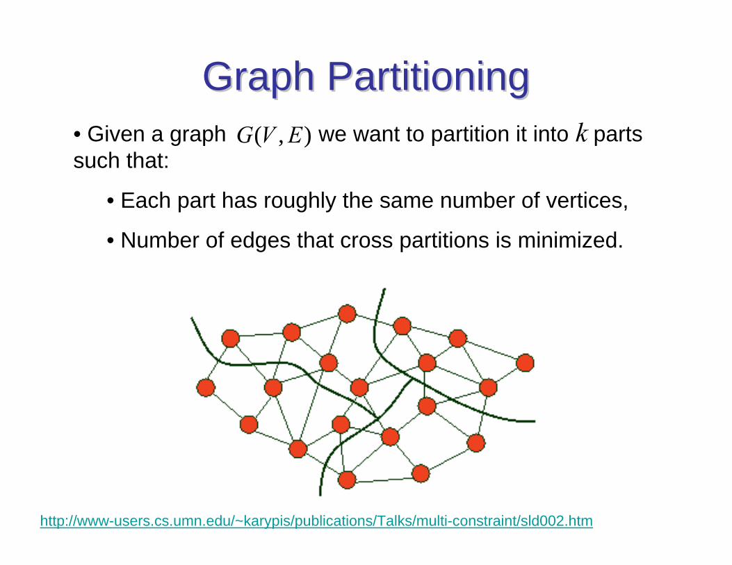
Graph PartitioningGraph Partitioning• Given a graph we want to partition it into parts such that:

• Each part has roughly the same number of vertices,

• Number of edges that cross partitions is minimized.

),( EVG k

http://www-users.cs.umn.edu/~karypis/publications/Talks/multi-constraint/sld002.htm

Mesh DecompositionMesh Decomposition• View mesh decomposition as having two aspects:

• Partitioning a graph,• Mapping the sub-domains to processors.

• Algorithms may• Address both issues, • Or simplify the problem by ignoring the latter.

• Whether this is an issue depends on target machine.• With very fast communications, e.g. the T3D, it's probably less important.• On a cluster of workstations it may be absolutely critical.


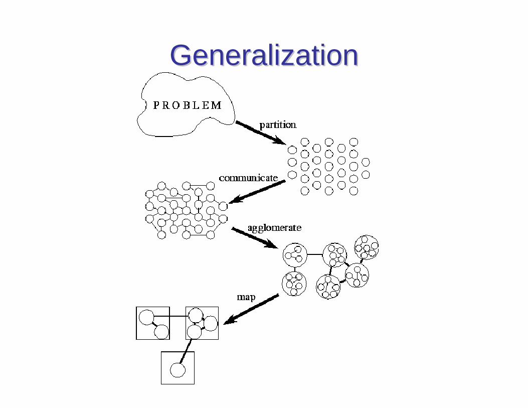
GeneralizationGeneralization

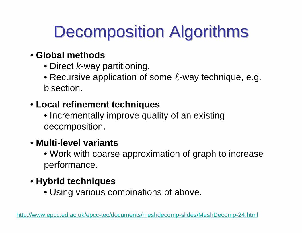
Decomposition AlgorithmsDecomposition Algorithms• Global methods

• Direct k-way partitioning.• Recursive application of some -way technique, e.g. bisection.

• Local refinement techniques• Incrementally improve quality of an existing decomposition.

• Multi-level variants• Work with coarse approximation of graph to increase performance.

• Hybrid techniques• Using various combinations of above.


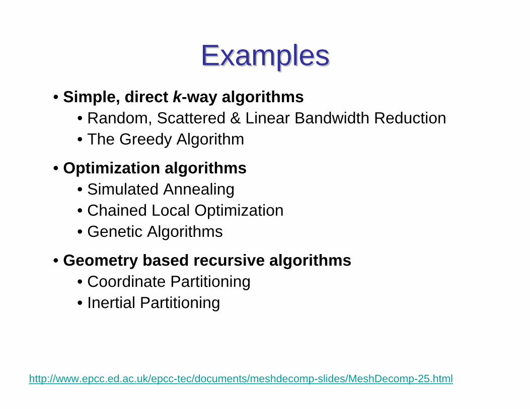
ExamplesExamples• Simple, direct k-way algorithms

• Random, Scattered & Linear Bandwidth Reduction• The Greedy Algorithm

• Optimization algorithms• Simulated Annealing• Chained Local Optimization• Genetic Algorithms

• Geometry based recursive algorithms• Coordinate Partitioning• Inertial Partitioning


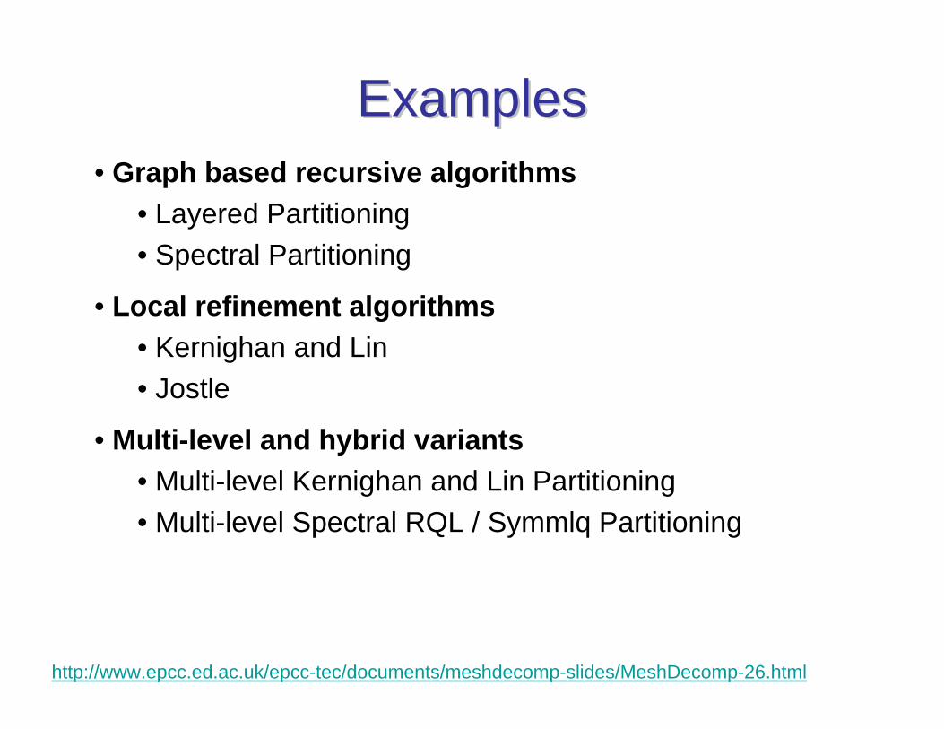
ExamplesExamples• Graph based recursive algorithms

• Layered Partitioning• Spectral Partitioning

• Local refinement algorithms• Kernighan and Lin• Jostle

• Multi-level and hybrid variants• Multi-level Kernighan and Lin Partitioning• Multi-level Spectral RQL / Symmlq Partitioning


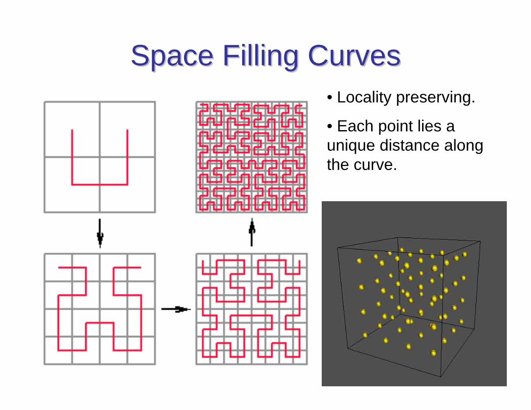
Space Filling CurvesSpace Filling Curves• Locality preserving.

• Each point lies a unique distance along the curve.

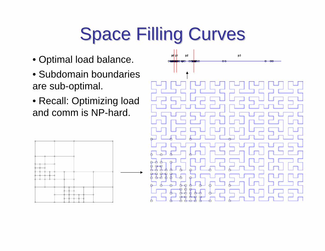
Space Filling CurvesSpace Filling Curves• Optimal load balance.• Subdomain boundaries are sub-optimal.• Recall: Optimizing load and comm is NP-hard.

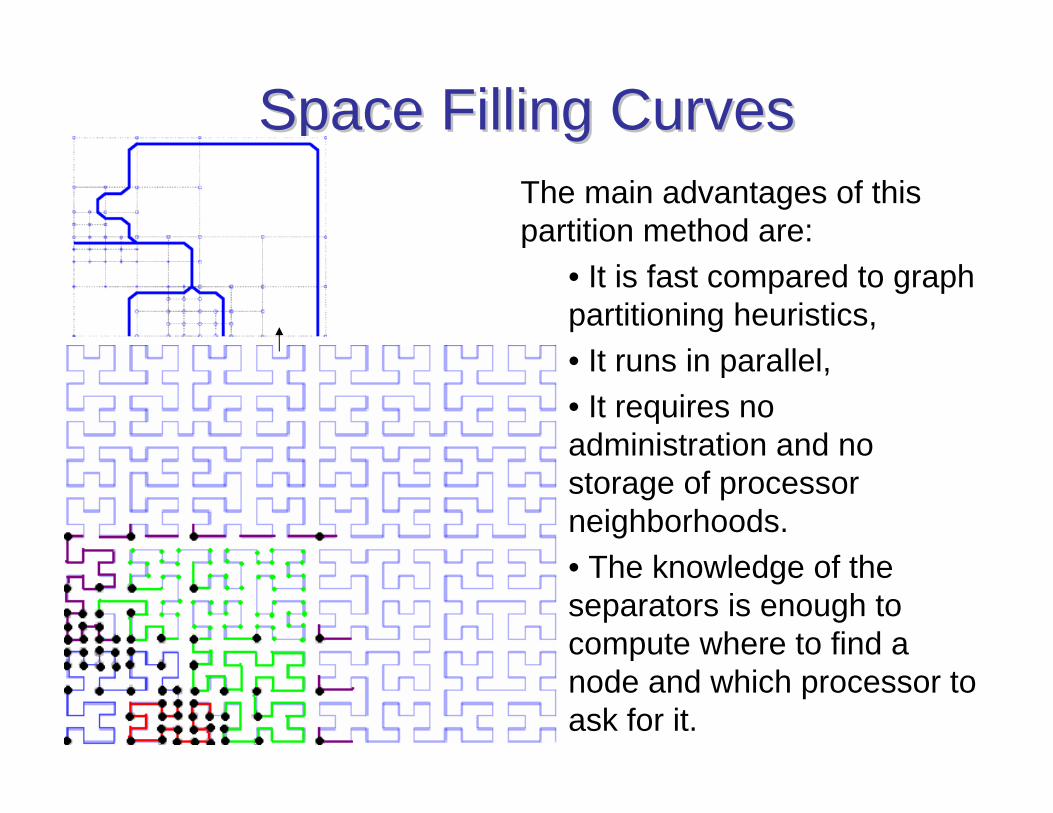
Space Filling CurvesSpace Filling CurvesThe main advantages of this partition method are:

• It is fast compared to graph partitioning heuristics,• It runs in parallel,• It requires no administration and no storage of processor neighborhoods. • The knowledge of the separators is enough to compute where to find a node and which processor to ask for it.

Parallel PDE ToolsParallel PDE Tools• Parallel ELLPACK -- Purdue University

• POOMA -- Los Alamos National Laboratory

• Overture -- Lawrence Livermore National Laboratory

• PADRE – LLNL, LANL

• PETSc -- Argonne National Laboratory

• Unstructured Grids -- University of Heidelberg

LinksLinks• A Software Framework for Easy Parallelization of PDE Solvers -- http://www.ifi.uio.no/~xingca/PCFD2000/Slides/pcfd2000/• Numerical Objects Online -- http://www.nobjects.com/Diffpack/• Xing Cai's home page at University of Oslo -- http://www.ifi.uio.no/~xingca/• Related Grid Decomposition Sites -- http://www.erc.msstate.edu/~bilderba/research/other_sites.html• Domain Decomposition Methods -- http://www.ddm.org/• People working on Domain Decomposition -- http://www.ddm.org/people.html• Unstructured Mesh Decomposition -- http://www.epcc.ed.ac.uk/epcc-tec/documents/meshdecomp-slides/• HPCI Seminar: Parallel Sparse Matrix Solvers -- http://www.epcc.ed.ac.uk/computing/research_activities/HPCI/sparse_seminar.html• METIS: Family of Multilevel Partitioning Algorithms -- http://www-users.cs.umn.edu/~karypis/metis/index.html• Multilevel Algorithms for Multi-Constraint Graph Partitioning -- http://www-users.cs.umn.edu/~karypis/publications/Talks/multi-constraint/sld001.htm• Structured Versus Unstructured Meshes -- http://www.epcc.ed.ac.uk/epcc-tec/courses/images/Meshes.gif• Domain Decomposition Methods for elliptic PDEs -- http://www.cs.purdue.edu/homes/mav/projects/dom_dec.html• Multiblock Parti library -- http://www.cs.umd.edu/projects/hpsl/compilers/base_mblock.html• Chaco: Software for Partitioning Graphs -- http://www.cs.sandia.gov/~bahendr/chaco.html• A Portable and Efficient Parallel Code for Astrophysical Fluid Dynamics -- http://astro.uchicago.edu/Computing/On_Line/cfd95/camelse.html• Links for Graph Partitioning -- http://rtm.science.unitn.it/intertools/graph-partitioning/links.html• A Multilevel Algorithm for Partitioning Graphs -- http://www.chg.ru/SC95PROC/509_BHEN/SC95.HTM• Multigrid Workbench: The Algorithm -- http://www.mgnet.org/mgnet/tutorials/xwb/mgframe.html• Domain DecompositionParallelization of Mesh Based Applications -- http://www.hlrs.de/organization/par/par_prog_ws/online/DomainDecomposition/index.htm• Parallel ELLPACK Elliptic PDE Solvers -- http://www.cs.purdue.edu/homes/markus/research/pubs/pde-solvers/paper.html• POOMA -- http://www.acl.lanl.gov/pooma/• Overture -- http://www.llnl.gov/CASC/Overture/• PADRE: A Parallel Asynchronous Data Routing Environment -- http://www.c3.lanl.gov:80/~kei/iscope97.1/iscope97.1.html• PETSc: The Portable, Extensible Toolkit for Scientific Computation -- http://www-fp.mcs.anl.gov/petsc/• UG Home Page -- http://cox.iwr.uni-heidelberg.de/~ug/• Space-filling Curves -- http://mrl.nyu.edu/~dzorin/sig99/zorin3/sld036.htm• Separate IMAGE for Basic foil 30 Two Space Filling Curves -- http://www.npac.syr.edu/users/gcf/cps615gemoct98/foilsepimagedir/030IMAGE.html• Using Space-filling Curves for Multi-dimensional Indexing -- http://www.dcs.bbk.ac.uk/~jkl/BNCOD2000/slides.html• The origins of fractals -- http://plus.maths.org/issue6/turner1/• Adaptive Parallel Multigrid Methods -- http://wissrech.iam.uni-bonn.de/research/projects/zumbusch/hash.html

Date post:	29-Aug-2019
Category:	Documents
Upload:	haquynh
View:	277 times
Download:	1 times

Partial Differential Equations - MGNetdouglas/Classes/cs521/pde/pde2004.pdf · Partial Differential...

Documents