PARTICLE FLUX TRANSFORMATION IN THE MESOPELAGIC WATER COLUMN: PROCESS ANALYSIS AND GLOBAL BALANCE A Dissertation by LIONEL GUIDI Submitted to the Office of Graduate Studies of Texas A&M University in partial fulfillment of the requirements for the degree of DOCTOR OF PHILOSOPHY May 2008 Major Subject: Oceanography
Transcript
PARTICLE FLUX TRANSFORMATION IN THE MESOPELAGIC
WATER COLUMN: PROCESS ANALYSIS AND GLOBAL
BALANCE
A Dissertation
by
LIONEL GUIDI
Submitted to the Office of Graduate Studies of Texas A&M University
in partial fulfillment of the requirements for the degree of
DOCTOR OF PHILOSOPHY
May 2008
Major Subject: Oceanography
PARTICLE FLUX TRANSFORMATION IN THE MESOPELAGIC
WATER COLUMN: PROCESS ANALYSIS AND GLOBAL
BALANCE
A Dissertation
by
LIONEL GUIDI
Submitted to the Office of Graduate Studies of Texas A&M University
in partial fulfillment of the requirements for the degree of
DOCTOR OF PHILOSOPHY
Approved by: Co-Chairs of Committee, George A. Jackson
Gabriel Gorsky Committee Members, Ellen Toby
Lars Stemmann Richard Sempéré Wilford Gardner
Head of Department, Piers Chapman
May 2008
Major Subject: Oceanography
iii
ABSTRACT
Particle Flux Transformation in the Mesopelagic Water Column: Process Analysis and
Global Balance. (May 2008)
Lionel Guidi, M.S., Université Pierre et Marie Curie (France)
Co-Chairs of Advisory Committee: Dr. George Jackson Dr. Gabriel Gorsky
Marine aggregates are an important means of carbon transfers downwards to the
deep ocean as well as an important nutritional source for benthic organism communities
that are the ultimate recipients of the flux. During these last 10 years, data on size
distribution of particulate matter have been collected in different oceanic provinces using
an Underwater Video Profiler. The cruise data include simultaneous analyses of particle
size distributions as well as additional physical and biological measurements of water
properties through the water column.
First, size distributions of large aggregates have been compared to simultaneous
measurements of particle flux observed in sediment traps. We related sediment trap
compositional data to particle size (d) distributions to estimate their vertical fluxes (F)
using simple power relationships ( )bdAF ⋅= . The spatial resolution of sedimentation
processes allowed by the use of in situ particle sizing instruments lead to a more detailed
study of the role of physical processes in vertical flux.
Second, evolution of the aggregate size distributions with depth was related to
overlying primary production and phytoplankton size-distributions on a global scale. A
new clustering technique was developed to partition the profiles of aggregate size
distributions. Six clusters were isolated. Profiles with a high proportion of large
aggregates were found in high-productivity waters while profiles with a high proportion
of small aggregates were located in low-productivity waters. The aggregate size and
mass flux in the mesopelagic layer were correlated to the nature of primary producers
iv
(micro-, nano-, picophytoplankton fractions) and to the amount of integrated chlorophyll
a in the euphotic layer using a multiple regression technique on principal components.
Finally, a mesoscale area in the North Atlantic Ocean was studied to emphasize
the importance of the physical structure of the water column on the horizontal and
vertical distribution of particulate matter. The seasonal change in the abundance of
aggregates in the upper 1000 m was consistent with changes in the composition and
intensity of the particulate flux recorded in sediment traps. In an area dominated by
eddies, surface accumulation of aggregates and export down to 1000 m occured at
mesoscale distances (<100 km).
v
ACKNOWLEDGMENTS
I would like to thank Piers Chapman, head of the Oceanography Department of
Texas A&M, Michel Glass, directeur de l’Observatoire Océanologique de Villefranche,
Louis Legendre, directeur de Laboratoire d’Océanographie de Villefranche et Louis
Prieur chef d’équipe, pour m’avoir accueilli dans leurs murs afin d’effectuer ma thèse
dans les meilleures conditions possibles between Texas A&M and Université Pierre et
Marie Curie in France.
Thanks to the members of the committee who evaluated my dissertation and for
the valuable discussions during the defense: Jean-Marc Guarini, Fauzi Mantoura,
Richard Sempéré, Ellen Toby, Wilford Gardner, Lars Stemmann, Gabriel Gorsky and
George Jackson.
Je remercie particulièrement les personnes qui m’ont suivi et encadré au cours de
ces 3 années : Lars stemmann pour tous ses conseils et sa grande patience malgré les
embûches administratives posées par les accords de cotutelle, Gaby Gorsky pour ses
idées, ses réunions du lundi, et sa perpétuelle bonne humeur et motivation me permettant
de toujours aller de l’avant, Marc Picheral pour sa rigueur et son amitié hors bureau,
Frédéric Ibanez pour ses solutions statistiques toujours très nombreuses. Finally, I would
like to thank George Jackson for involving me in this great adventure during these nine
months in Texas. Thanks for your patience, all the coffee breaks and following
discussions. You always kept me motivated even during the most doubtful period of my
dissertation.
Je tiens également à remercier toutes les personnes qui m’ont entouré au cours de
ces 3 années, m’ont permis d’expérimenter la vie à bord d’un bateau de recherche et sans
qui cette thèse aurait été un peu moins passionnante (Hervé Claustre et Antoine
Sciandra, ainsi que toutes les personnes embarquées sur BIOSOPE, Franco Decembrini
and all his team during the CIESM cruise in Italy and Dave Checkley and others during
the SCRIPPS cruise off the Californian coast). Merci aussi à tous les membres de
l’Observatoire Océanologique de Villefranche et du Oceanography Department of Texas
vi
A&M (especially the Ph.D. students), trop nombreux pour être nommés mais sans qui
ces années n’auraient pas été aussi « fructueuses ».
Finally, I am thankful to my roommates (Jake, Michael and Ryan) for teaching
me about life in Texas. Merci aussi mes colloc Français (Jon ; sans qui la soutenance
n’aurait pas eu lieu, Aurélie, Fanny, et Flo quasi colloc). Merci bien sur à mes parents et
ma sœur pour leur soutient permanent. Je terminerai en remerciant Solange qui
m’accompagne, m’épaule et me motive depuis le début de ce projet malgré toutes les
III PARTICLE SIZE DISTRIBUTION AND FLUX IN THE MESOPELAGIC: A CLOSE RELATIONSHIP............................................ 51
3.1. Introduction........................................................................................... 51 3.2. Material and methods............................................................................ 54 3.3. Results................................................................................................... 58 3.4. Discussion............................................................................................. 62 3.5. Conclusion ............................................................................................ 69
viii
Page CHAPTER
IV PRIMARY PRODUCER COMMUNITY EFFECT ON PRODUCTION AND EXPORT OF LARGE AGGREGATES: A GLOBAL ANALYSIS. .................................................................................. 71
4.1. Introduction........................................................................................... 71 4.2. Material and methods............................................................................ 73 4.3. Results................................................................................................... 81 4.4. Discussion............................................................................................. 90
V VERTICAL DISTRIBUTION OF AGGREGATES (>110 µM) AND MESOSCALE ACTIVITY IN THE NORTHEASTERN ATLANTIC: EFFECTS ON THE DEEP VERTICAL EXPORT OF SURFACE CARBON .................................................................................... 96
APPENDIX A ARTICLE A .......................................................................................... 147
APPENDIX B ARTICLE B........................................................................................... 148
APPENDIX C ARTICLE C........................................................................................... 149
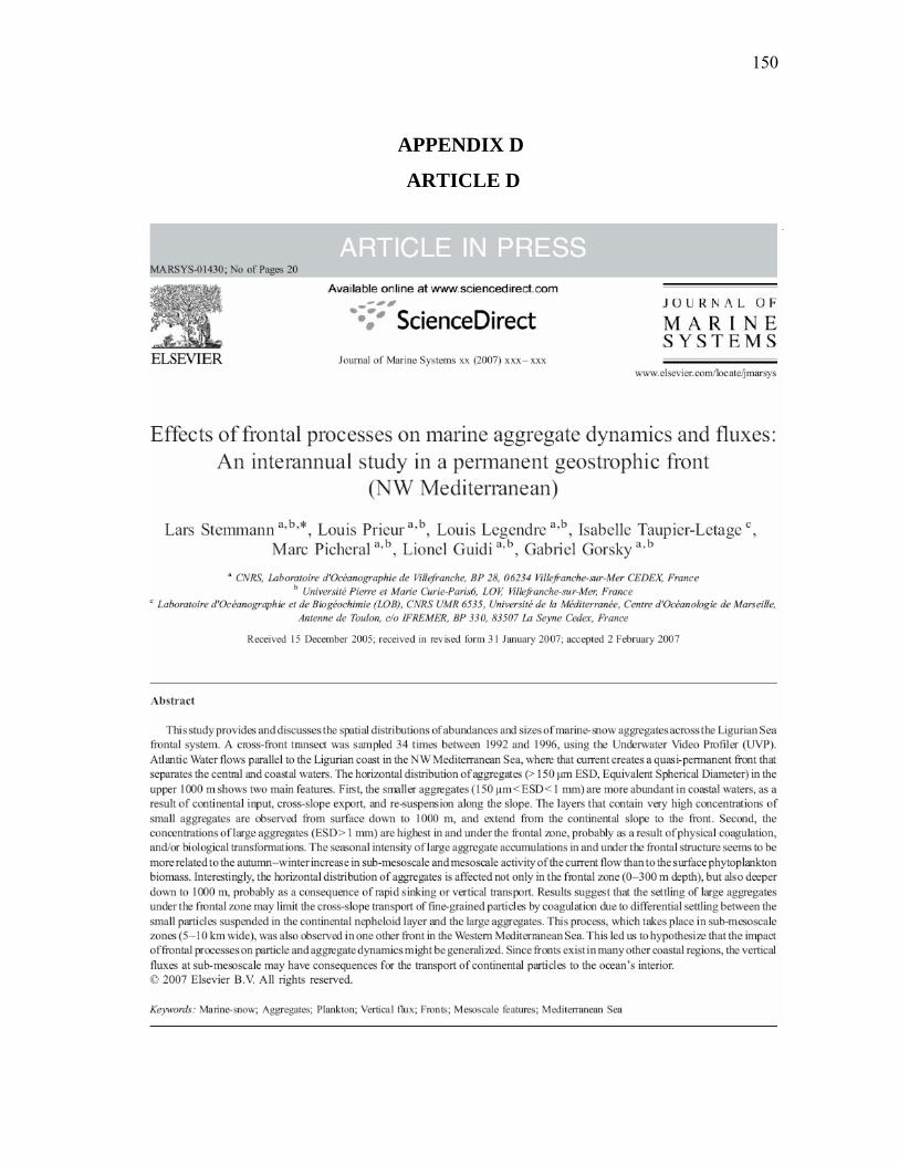
APPENDIX D ARTICLE D .......................................................................................... 150
APPENDIX E ARTICLE E ........................................................................................... 151
APPENDIX F ARTICLE F............................................................................................ 152
VITA ............................................................................................................................... 153
ix
LIST OF TABLES Page
Table 1: Summary of parameters used for the pixel to millimeter size conversion. The water volume recorded by each image and the minimum aggregate size that each UVP generation can measure is also given. ............................... 25
Table 2: Definition of the 27 aggregate size classes used in this work. ......................... 30
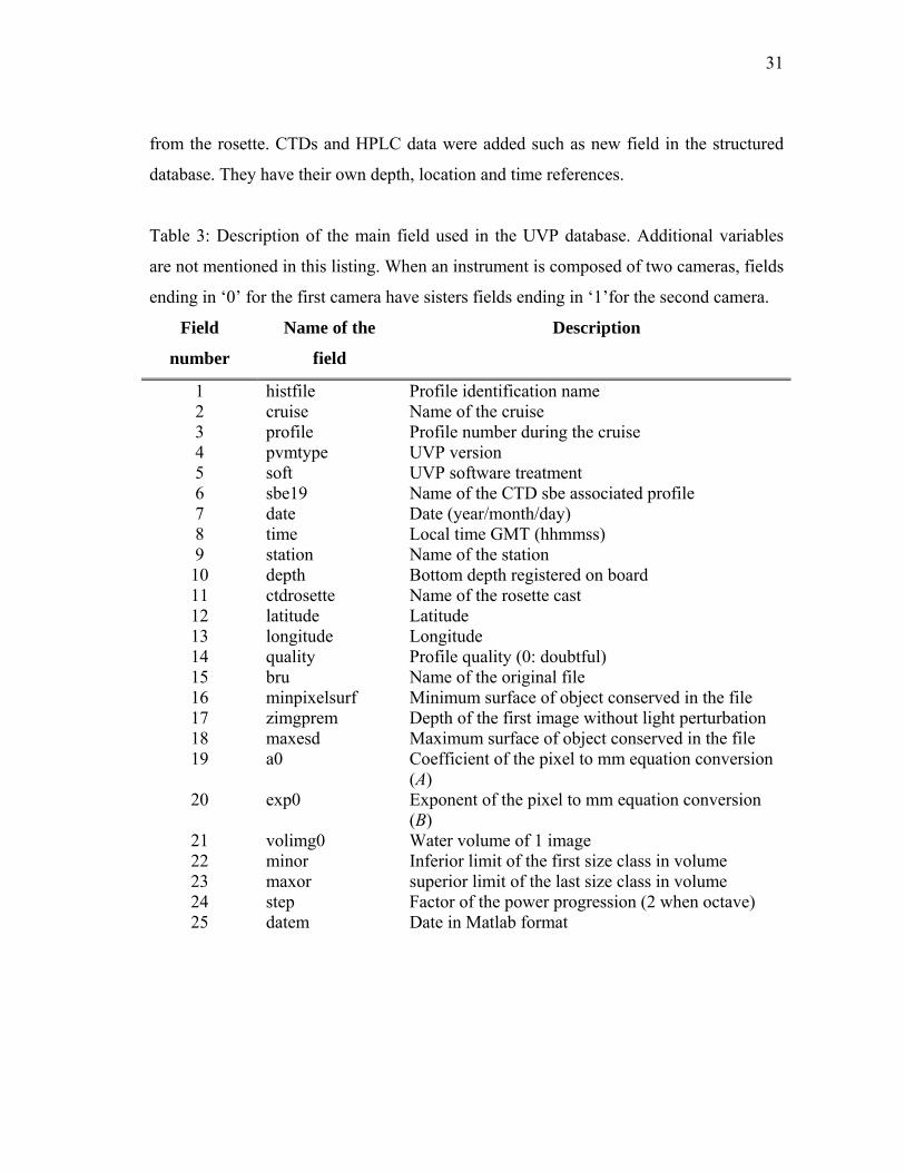
Table 3: Description of the main field used in the UVP database. Additional variables are not mentioned in this listing. When an instrument is composed of two cameras, fields ending in ‘0’ for the first camera have sisters fields ending in ‘1’for the second camera.............................................. 31
Table 4: Comparisons of the Calinski and Harabasz index and, RST method sensitivity to 4 different cluster analyses, (S) simple link, (C) complete link, (U) UPGMA and, (W) Ward’s minimum variance procedure, considering the number of groups in the datasets. The total number of tested dataset by clustering analyses and number of groups is 27. ‘-1’ and ‘-2’ denote that the method detected one or two groups in less in comparison to the true number of groups while ‘+1’,‘+2’ and ‘+3’ mean that the method identified one, two or three or more groups in more in comparison to the true number of groups ......................................................... 42
Table 5: Two examples showing the effects of outliers on Calinski and Harabasz index (C&H) and RST technique using the dataset generated by the algorithm of Milligan and Cooper (1985). The example a) is composed by 4 clusters whereas the example b is composed by 3 clusters. Both examples contain 50 observations and 10 outliers (20%) in the dataset. The real clusters of data are shown in the first part of the table and the corresponding results obtained with the C&H index and the RST are shown in the second and third part of the table, respectively. .......................... 43
Table 6: Non exhaustive literature review on the determination of the number of cluster using Fisher’s dataset. ........................................................................... 48
Table 7: List of parameters and their dimension (M for mass, L for length, T for time).................................................................................................................. 52
Table 8: Definition of the size range and volume sampled characteristics of the 3 different Underwater Video Profilers (UVP) used in this study....................... 54
Table 9: Location, position, and duration of the deployments of the sediments trap used in this study. References: A- (Guieu et al. 2005); B-(Stemmann et al. 2002); C -Miquel and Gasser, submitted.............................. 56
x
Page
Table 10: Coefficient (A) and exponent (b) and their associated standard deviation (STD) of the empirical relationship between the aggregate size and their related mass, particulate organic carbon (POC), particulate inorganic carbon (PIC) and particulate organic nitrogen (PON) fluxes determinate by minimization of the fluxes estimation by the Underwater Video Profiler (UVP) and the sediment traps measurement, n=118. .......................... 60
Table 11: Distribution of profiles within clusters for each cruise. The numbers in the C columns indicated the number of profiles that fall into the cluster......... 78
Table 12: Spearman correlation between 4 parameters of the aggregate size distribution (n=410), all correlation were significant ....................................... 81
Table 13: Phytoplankton size structure (% of fmicro, fnano, fpico) and integrated chlorophyll a content (Ba) in the Ze compared to the total aggregate flux below the euphotic layer at 400 m: F400......................................................... 86
Table 14: Components from PCA of descriptors, sorted by their decreasing r², correlation with the flux at 400m; r² values and probability (p) associated. Component selected for the PCR are in bold. Model’s coefficient and their confidence interval after the multiple regression between the 7 descriptors (fmicro, fnano, fpico,Bmicro,Bnano,Bpico,Ba) and the aggregate flux at 400m (F400) summarized in the 2 last columns..................... 90
Table 15: Cruises and UVP characteristic uses for all profiles ...................................... 100
Table 16: Spearmen correlation coefficient between integrated aggregate concentrations and integrated pigment concentrations in the 40-60 m layer. ............................................................................................................... 109
xi
LIST OF FIGURES Page
Figure 1: Biological pump and processes regulating the flux of particles in the ocean. CO2 fixed during photosynthesis by phytoplankton can be transferred below the surface mixed layer via three major processes, (1) passive sinking of particles, (2) physical mixing of particulate and dissolved organic matter, and (3) active transport by zooplankton vertical migration. The remineralization returns carbon and nutrients to dissolved forms (Figure from Buesseler et al. 2007a)...................................... 3
Figure 2: UVP video images with macrozooplankton groups; appendicularians
(App.), Thaliacae (Thal.; salp and doliolid), Fish, Haliscera spp medusa (Hal.), Solmundella bittentaculata (Sol.), Aglantha spp. (Agl.) Aeginura grimaldii (Gri.) and ‘other medusae’ (Med. ) , chaetognath (Chaet.), lobate ctenophore (Lob.), cydippid ctenophore (Cyd,), siphonophore (Siph.), crustaceans (Crust.; decapod and amphipod), single cell sarcodine grouped by four (RadioCS.), colonial radiolarians (RadioC.), colonial radiolarians with double line (RadioCD.), Phaedorian (Phaeo.), single cell sarcodine with spines (Spine.), double cell sarcodine with spines (Spine2.), spheres (Sphere.) and sarcodine with hairs (Stars.). The scale bar represents approximately 1 cm. Additional images can be viewed at http://www.obs-vlfr.fr/LOV/ZooPart/Gallery/. (Figure from Stemmann et al. Accepted) ........ 4
Figure 3: Floating sediment trap deployment during the BIOSOPE cruise in the Southeastern Pacific ....................................................................................... 18
Figure 4: Illustration of the last version of the Underwater Video Profiler................... 22
Figure 5: Example of data used for the calculation of the conversion equation from pixel to millimeter size measurement. Each color corresponds to an object type.................................................................................................. 24
Figure 6: Example of curve of light intensity registered at one point of the grid used for the calculation of the water volume sampled by one image............. 25
Figure 7: Complete set of light intensity curve obtained at every point of the grid. The greens curves correspond to the light intensity spectrum from the stroboscope 1. Reds light intensity spectrum came from stroboscope number 2. Blue curves correspond to the sum of the 2 stroboscopes. .................................................................................................. 26
xii
Page
Figure 8: Mean aggregate size distribution obtained with 4 UVP generations between 75 and 150 m. A) Combined profiles made by UVP 4a and 2c. B) Aggregate size distribution from the DYFAMED site in the Mediterranean Sea in May 1995 for UVP 2a and May 2003 for PVM 4a. C) Aggregate size distribution from the DYFAMED site from UVP 3b deployment in October 1993 and from UVP 2a in October 1993 and 1994. ............................................................................................................... 28
Figure 9: Profiles location of UVP (black circles), CTD (red dots), and pigment profiles (green squares) .................................................................................. 32
Figure 10: Schematic representation of the successive steps of the Random Simulation Test (RST).................................................................................... 37
Figure 11: Result of the Calinski and Harabasz stopping rules applied on the Iris dataset between 2 and 21 clusters solutions. .................................................. 39
Figure 12: (A) Frequencies distribution of the number of cluster for the ecological dataset of Beaugrand et al. (2002). (B) Dendrogram of calanoid copepod species resulting from the flexible hierarchical clustering method used by Beaugrand et al., (2002). Underlined taxa have indicator value inferior to 25%. Groups (at the distance cut-off level of 1.152) are indicated in pale grey. Subgroups (distance cut-off level of 0.53) are indicated in dark grey. Numbers underlined and in italic represent the number of taxa for each group. Some characteristics of each group are given in grey and italic. Underlined species are species rarely collected by the Continuous Plankton Recorder survey. The dashed grey lines are cut-off levels empirically chosen by Beaugrand et al. (2002). Dark lines are the cut-off levels determined by the Random Simulation Test (0.56 and 0.45) ..................................................................... 45
Figure 13: Location of all Underwater Video Profiler (UVP) profiles (red crosses) and associated sediment trap deployments (black stars). There were 1254 total profiles and 11 associated sediment trap locations. ...................... 55
Figure 14: Comparison of measured sediment trap mass flux with that calculated using size spectra and Alldredge and Gotschalk (1988) relationships (n=118). Symbols represent trap deployments depths: 100 m - open squares, 200m - open circles, 300m - open stars, 400m - black dots and 1000m - crosses. ............................................................................................. 58
xiii
Page
Figure 15: Measurement of the mass (A), particulate organic carbon (POC: B), particulate inorganic carbon (PIC: C) and particulate organic nitrogen (PON: D) fluxes by sediment traps, compared to the estimation of the mass, POC, PIC, PON fluxes using the UVP and the relationships between the aggregates size and the previous fluxes (cf Eq. 15,16,17 and 18) n=118. Symbols represent trap deployments depths: 100 m - open squares, 200m - open circles, 300m - open stars, 400m - black dots and 1000m - crosses................................................................................ 59
Figure 16: Ratio of estimates and measurements of the A) mass fluxes, B) POC fluxes, C) PIC fluxes, D) PON fluxes as function of the depth of sediment traps................................................................................................. 61
Figure 17: Residual error ∆F as a function of values of A, b for the mass flux Fm. The best fit values were A=109.5 and b=3.52. Darker regions represent greater values for ∆F in mg m-2 d-1. The crosses correspond to the values calculated during the jackknife error analysis. They are all located in the area where the residues are the smallest. ................................. 62
Figure 18: A) Particle settling speed function of particle diameter measured by different authors (from Stemmann et al. 2004b). Circle: (Smayda 1970), triangle: (Shanks and Trent 1980), diamond: (Carder et al. 1982), square: (Azetsu-Scott and Johnson 1992). Empirical relationships, 1—(Alldredge and Gotschalk 1988), 2—(Alldredge and Gotschalk 1989), 3—(Syvitski et al. 1995), 4—(Diercks and Asper 1997). Settling speeds calculated using the coagulation model (Stemmann et al. 2004b) with different parameter values (5—
08.0=∆ρ , D=2.33; 6— 01.0=∆ρ , D=1.79) are also reported. The regression line 7 is the settling speed predicted by Stokes Law. The dashed line 8 is the settling speed calculated in this paper. B) Typical number spectrum from the UVP database profiles. C) Normalized cumulative flux calculated on the number spectrum (B) with the mass flux relationship Eq. 20, the black line represents the 50% of the mass flux.................................................................................................................. 66
Figure 19: Sediment trap mass flux measurement below the euphotic zone in mg m-2 d-1 along 150°W (black asterisk) redrawn from (Raimbault et al. 1999) compared to estimated mass flux from aggregates size distribution along 180°W (gray bars)............................................................. 68
xiv
Page
Figure 20: Estimation of the mass flux for a radial 180°W in the Equatorial Pacific Ocean, based on the size aggregate distribution. A=109.5 and b=3.52 for the size to mass flux relationship (Table 10). The dots correspond to the sampling grid. .................................................................... 69
Figure 21: Samples location of UVP (black circles), CTD (red dots), and pigment profiles (green squares) .................................................................................. 74
Figure 22: Comparison of different measures of the number distribution: b (slope of the number distribution), d25 (Equivalent spherical diameter (ESD) relative to 25% of the cumulative volume distribution), d50 (ESD relative to 50% of the cumulative volume distribution), d75 (ESD relative to 75% of the cumulative volume distribution). An example of measurements on one distribution (A and B), the 4 measurements correspond to 1 point in C). A) Cumulative volume distribution. B) Number spectrum n from which b was calculated. C) Relationship between b and d25, d50, and d75. ...................................................................... 76
Figure 23: Slope profiles based on the particle size distribution, divided into 6 patterns. The Euclidean distance and the flexible link were used for the classification. Number of clusters were selected with the random simulation test (RST) (A to F for clusters 1 to 6)........................................... 83
Figure 24 : Location of the 6 patterns of the slope profiles based on the particle size distributions of aggregates in the water column (A to F for clusters 1 to 6).............................................................................................................. 84
Figure 25: Phytoplankton size classes related to the estimated flux at 400 m. A) Micro-phytoplankton fraction (fmicro) in color: chlorophyll a integrated over Ze (Ba) versus total flux at 400 m (F400). B) Same parameters for nano-phytoplankton (fnano) in color. C) Same parameters for pico-phytoplankton (fpico) in color.. ........................................................................ 87
Figure 26: Flux in the mesopelagic zone. A) Ternary plot of total aggregate flux at 400 m (F400) B) Ternary plot of the aggregate mass flux fraction estimated at 1000 m compared to the estimated aggregate mass flux below Ze. Both calculation are related to the phytoplankton structure in Ze (fmicro, fnano, fpico in fractions)...................................................................... 88
Figure 27: Selected components (C) of PCA for PCR. The solid line corresponds to the coefficient of determination R² of the multiple regression. The dashed line corresponds to the R² progression by successive component addition. ....................................................................................... 89
Figure 28: Flux measurement vs flux modeled by the PCR, n=193................................ 91
xvPage
Figure 29: Study area in the Northeastern Atlantic. The dashed line is the approximate location of the zone of discontinuity of the winter mixed layer associated with subduction of mode water masses. .............................. 98
Figure 30 : Sampling grid during the three POMME cruises. Locations of CTDs, shown by open circles, UVP stations by closed circles, and long stations and sediment traps by open squares. ................................................. 99
Figure 31: Geopotential anomalies at 300m calculated from hydrographic data during (A) winter, (B) spring, and (C) summer calculated from the sampling grid. The squares represent the locations of the UVP profiles. The black circles represent the positions where high stocks of aggregates were observed in the mesopelagic layer during winter and spring. These positions correspond to the locations where the 400-800 m integrated concentrations exceeded 5 times the surrounding integrated concentrations. These calculations were not performed for the summer cruise because of the lack of data deeper than 500 m. ............. 101
Figure 32: 3D maps of density field during (A) winter, (B) spring, and (C) summer and vertical sections of sea-water density in (D) winter, (E) spring, and (F) summer as inferred from all the CTDs. The MLD is marked by the black continuous line in both the section and 3D maps and the mode water is located between the 2 white continuous lines. The station numbers where the UVP was deployed are given above each section. The ship tracks are given on the maps on the left of each section. The continuous and dotted lines on each map are repeated under each section in order to help the reader to localize itself. The arrows point at the start of the track. ............................................................ 103
Figure 33: Median vertical profiles, and first and third quartiles, of aggregate mass during the three cruises: winter (n=36), spring (n=43) and summer (n=41). Note that for the summer profiles, median values deeper than 500 m were calculated using only 6 available UVP profiles.......................................................................................................... 105
Figure 34: 3D maps of seasonal changes in the vertical distribution of aggregates in (A) winter, (B) spring, and (C) summer, and vertical sections of aggregate distribution along the ship tracks in (D) winter, (E) spring, and (F) summer, in mg dry wt m-3. The station numbers where the UVP was deployed are given above each section. The color scale emphasizes variability at the lower end of the concentration range. The depth of the isomass of aggregates 8 mg m-3 is given by the white line. The ship tracks are given on the maps on the left of each section. The continuous and dotted lines on each map are repeated under each section in order to help the reader to localize itself. The arrows point at the start of the track. ..................................................................................... 107
xvi
Figure 35: Vertically integrated concentrations of aggregates as a function of vertically integrated Chl a in three phytoplankton groups during the different cruises for the 0-200 m layer. ........................................................ 108
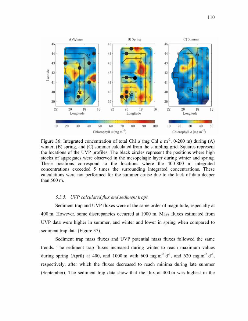
Figure 36: Integrated concentration of total Chl a (mg Chl a m-2, 0-200 m) during (A) winter, (B) spring, and (C) summer calculated from the sampling grid. Squares represent the locations of the UVP profiles. The black circles represent the positions where high stocks of aggregates were observed in the mesopelagic layer during winter and spring. These positions correspond to the locations where the 400-800 m integrated concentrations exceeded 5 times the surrounding integrated concentrations. These calculations were not performed for the summer cruise due to the lack of data deeper than 500 m. ........................................ 110
Figure 37: Figure modified from Guidi et al. (in revision). Comparison between UVP potential mass fluxes and mass fluxes from sediment traps at (A) 400 m and (B) 1000 m. Potential fluxes from UVP using Alldredge and Gotschalk (1988) in black circles and using relationship presented in chapter III in red circles. The sediment traps were corrected for trapping efficiency, which was estimated to range from 20 to 50% (Guieu et al. 2005)........................................................................................ 111
Figure 38: From Uitz et al. 2006. Phytoplankton community composition for June 2000 (SeaWiFS composite): (a–c) phytoplankton fractions (fmicro, fnano and fpico in %) within the 0–1.5 Ze layer, and (d–f) integrated contents within the same layer (Bmicro, Bnano and Bpico in mg m−2). Coastal areas (less than 200 m deep), large lakes and inland seas are represented in white...................................................................................... 123
1
CHAPTER I
1 GENERAL INTRODUCTION Understanding the effect of food web dynamics on biogeochemical cycles is the
central issue of the international IMBER (Integrated Marine Biogeochemistry and
Ecosystem Research) program. The subjects developed in this PhD dissertation are
central to this goal, dealing with the transfers of matter across oceans interfaces.
Biogeochemical processes differ among environments such as continental slopes,
regions with active convection, regions with dynamic mesoscale features enhancing
local biological production and oligotrophic central gyres. There is a general agreement
that the response of the biogeochemical cycles to environmental changes needs to be
understood better. Studies that compare processes impacting the characteristics and the
vertical transfer of particulate matter in different environments may significantly
ameliorate our knowledge on the fate of the surface biological production.
One of the results of international programs studying vertical fluxes, such as
VERTEX and Joint Global Ocean Flux Study (JGOFS), was that an average of 10% or
more of the surface oceanic production is exported below the mixed layer depth. The
main export is by large particulate matter, notably aggregates with diameters> 100 µm.
However, only 1 to 10% of this matter falls below 1000 m depth, where is isolated from
the surface for long periods (Berelson 2001; Martin et al. 1987; Suess 1980).
Marine aggregates are a key factor of the ocean’s carbon cycle at different scales.
At the macroscale, marine aggregates are an important means of transferring carbon
downwards to the deep ocean by the way of the biological pump. At the microscale, they
provide dissolved and particulate food to micro and macro-organisms living in the
aphotic layer of the ocean (Alldredge 2000; Lampitt et al. 1993b). Aggregates are an
especially important nutritional source for benthic communities that are the ultimate
recipient of the flux (Buesseler et al. 2007a; Figure 1).
This dissertation follows the style of Limnology and Oceanography.
2
The largest fraction of exported surface production is remineralized in the meso-
pelagic zone by mechanisms about which we know little (Boyd and Trull 2007;
Buesseler et al. 2007b; Stemmann et al. 2004b). Most coupled climate biogeochemical
models do not consider the interaction between dissolved matter, colloids, aggregates,
and organisms. They use empirical parameterizations which ignore the importance and
details of physical and biological processes involved in the carbon cycle. Climate
simulations are very sensitive to such parameterizations (Gehlen et al. 2006). One of the
most important parameters is particle length, which can determine settling speed. As a
result, the international modeling community is working to develop more realistic
models of sub-euphotic zone particle transformation processes. Several models of
vertical fluxes suggest that coagulation, zooplankton feeding on aggregates, and
bacterial degradation, play important roles in particle transformation and flux reduction
(Gehlen et al. 2006; Jackson 2001; Quere et al. 2005; Stemmann et al. 2004b). However
they all lack data to constrain the model structures or to adjust their parameters values.
Despite progress resulting from multiple international programs, important
questions remain.
• What are the settling velocities of in situ aggregates and how can they be
related to their sizes? Can aggregate size be related to aggregate flux?
Characteristics of surface aggregates are quite well known; however, little information is
available on the nature of deeper particles. Our best tool for collecting deep particles has
been the sediment trap, which integrates over many types and settling velocities of
particles and provides information about bulk material rather than those of individual
particles. Making it more difficult to characterize particles is that most aggregates are
fragile and difficult to sample individually.
• What mechanisms are responsible for aggregate production, transformation
and export in the water column?
Processes of aggregate production and degradation are essential to understand.
Efficiency of carbon sequestration to the deep ocean is related to these processes. Large
uncertainties on mechanisms responsible for aggregate transformation remain.
3
• What is the spatial variability of carbon flux? Does it need to be taken into
account in order to obtain more realistic estimation of carbon flux at global scale?
The global and regional variability of the carbon export to the deep ocean is not well
understood. Its importance in assessing carbon export at the global scale is not well
appreciated.
Figure 1: Biological pump and processes regulating the flux of particles in the ocean. CO2 fixed during photosynthesis by phytoplankton can be transferred below the surface mixed layer via three major processes, (1) passive sinking of particles, (2) physical mixing of particulate and dissolved organic matter, and (3) active transport by zooplankton vertical migration. The remineralization returns carbon and nutrients to dissolved forms (Figure from Buesseler et al. 2007a).
4
One way to address the problems of in situ size estimation of particles is the use
of optical methods. These methods allow a detailed description of the aggregate size
spectra but do not allow their physical sampling. Here we are using results collected
during the last two decades by an instrument built at the Laboratoire Océanologique of
Villefranche sur mer called the Underwater Video Profiler (UVP). The instrumented
platform acquired data simultaneously on physical and biological properties, particles
size and macrozooplankton distribution (Figure 2).
Figure 2: UVP video images with macrozooplankton groups; appendicularians (App.), Thaliacae (Thal.; salp and doliolid), Fish, Haliscera spp medusa (Hal.), Solmundella bittentaculata (Sol.), Aglantha spp. (Agl.) Aeginura grimaldii (Gri.) and ‘other medusae’ (Med.) , chaetognath (Chaet.), lobate ctenophore (Lob.), cydippid ctenophore (Cyd,), siphonophore (Siph.), crustaceans (Crust.; decapod and amphipod), single cell sarcodine grouped by four (RadioCS.), colonial radiolarians (RadioC.), colonial radiolarians with double line (RadioCD.), Phaedorian (Phaeo.), single cell sarcodine with spines (Spine.), double cell sarcodine with spines (Spine2.), spheres (Sphere.) and sarcodine with hairs (Stars.). The scale bar represents approximately 1 cm. Additional images can be viewed at http://www.obs-vlfr.fr/LOV/ZooPart/Gallery/. (Figure from Stemmann et al. accepted).
5
The objective of my PhD work has been to describe large aggregate size
distributions in the oceans. These distributions were used to highlight important
mechanisms at the origin of aggregate formation and export at global and regional scale.
The current knowledge on particle dynamics is synthesized into the following
paragraphs. Following the introduction, the manuscript will be divided in a
methodological chapter and three additional chapters addressing the 3 previous questions
on particles characteristics, formation and fate in the upper kilometer of the ocean. The
last chapter will present a general conclusion.
1.1. What do we know about aggregate properties?
1.1.1. Aggregate size
There are many ways to characterize particle size, ranging from wet weight to
carbon content to volume to radius. In this dissertation, size will usually refer to
diameter (d) as determined using particle images.
Particles found in oceanic ecosystems range in diameter from 1 nm (“almost
dissolved” colloids) to a few millimeters (diatom chains) or centimeters (cyanobacterial
filaments). Three size classes of organic aggregates have often been distinguished in the
past: macroscopic aggregates (d>500 µm), such as macroaggregates, marine snow, and
lake snow, microscopic aggregates (1 < d < 500 µm), also known as “microaggregates”
and submicron particles (d <1 µm; Simon et al. 2002). Macro- and microaggregates are
generally formed by phytoplankton; their sizes can depend on the trophic state of the
planktonic system, the season and the geographic region. Their compositions can vary
from being individual algal cells to being composed of multiple particles embedded in a
mucilaginous matrix (Alldredge and Silver 1988). The large size range covered by these
organic aggregates implies that many complex physical, chemical, biological and
specific microbial processes are involved in their formation and decomposition.
The aggregate size distribution is a continuum. Particle abundances in the water
column can usually be described as a function of particle diameter. This relationship is
not simple because aggregates are porous objects with porosity increasing with their size
and because they are formed from different constituents having different densities.
6
Fractal scaling has been used in order to describe these relationships (Jackson 1998; Li
and Logan 1995).
1.1.2. Mathematical description of particle size spectrum
Particle abundances as a function of size can be described using a size
distribution. If N(s) is number concentration of particles greater than a size s, then n(s)=
-dN/ds. While both describe particle distributions, the terms cumulative size distribution
and differential size distribution are used for N(s) and n(s). References to size
distribution or number size distribution here are to n(s). The number spectrum is usually
estimated as n(s) ≈(N(s)-N(s+∆s))/ ∆s, where ∆s is a small size range. Any measure of
size such as volume, diameter, or radius, can be used as the size, although the values and
units do change with the measure.
Previous research has shown that oceanic particles tend to follow a power law
distribution function over the µm to mm size range (McCave 1984; Sheldon et al. 1972).
This kind of distribution can be translated as the following mathematical equation and is
retrieved from UVP images:
( ) bdkdn ⋅= (Eq. 1)
where k and b are constants. The exponent (b) is also defined as the slope of number
spectrum when the equation 1 is log transformed. This slope is commonly used as a
descriptor of the shape of the aggregate size distribution (Brun-Cottan 1971; McCave
1975; Sheldon et al. 1972).
The information of this simple metric can be limited when the log-transformed
aggregate size distribution is not linear. The importance of large aggregates in some
systems can be missed using only the slope of a defined number spectrum. The number
spectrum can be transformed to a volumetric or a mass spectrum that emphasizes the
importance of large particles in mass distribution. Large aggregates may be negligible by
number but they can represent more than 50% of the total mass of aggregates
(Stemmann et al. submitted). Diameter is a useful particle descriptor because it can
describe multiple particle properties such as mass and settling speed or flux (Alldredge
and Gotschalk, 1988, Guidi et al in revision), rate of colonization by microbes and
7
zooplankton (Kiørboe 2001; Kiørboe et al. 2002) and coagulation rate (Jackson and
Lochmann 1992). Biogeochemical activity such as aggregate remineralization by
bacterial activity or zooplankton consumption can also be a function of the same length
(Kiorboe and Thygesen 2001; Ploug and Grossart 2000).
Diameter is an important descriptor of the system and will be the common descriptor
used in the following work.
1.1.3. Mathematical description of particle fractal dimension
The relationships between fractal geometry and the exponents for the diameter in
the power relationships between particle mass and diameter have been used to estimate
fractal dimensions (D) (Logan and Wilkinson, 1990) and the vice versa (Jackson et al.,
1997). If the particle size is given by particle diameter (d), then its mass (m) is:
(Eq. 2) Ddadm ⋅=)(
Calculated fractal dimensions for natural surface water and laboratory aggregates
have been estimated to be between 1.3 and 3.75 (Jackson et al. 1997; Jiang and Logan
1991; Li and Logan 1995). A value of 3 indicates that the density is constant with size.
Values of D >3 can arise from measurement errors or use of an inappropriate model
when analyzing observations. Surface marine snow typically has a fractal dimension (D)
between 1.3 and 2.3. Much less is known about aggregates in the midwater layers.
Fractal geometry also allows estimation of the porosity of aggregates, which is
inversely related to the fractal dimension and a function of size (Logan and Wilkinson
1990). The porosity is important in controlling the aggregate’s sinking rate, the flux of
water through the aggregate moving relative to the surrounding water, and the flux of
nutrients and substrates to and from the microorganisms colonizing the aggregate’s
surface (Alldredge and Gotschalk 1988; Logan and Hunt 1987; Ploug 2001).
8
An innovative approach based on comparison of aggregate size distribution
and flux measurement by sediment trap was developed to assess the fractal dimension
of aggregates during this work and will be exposed in Chapter III of the dissertation
(Guidi et al. in revision).
1.2. Aggregate sources
Settling material can exist as isolated source particles or incorporated in a more
complex structure termed “marine snow” (Silver et al. 1978; Suzuki and Kato, 1953). A
marine snow particle is an aggregate larger than 500 µm; marine snow is ubiquitous in
the world’s ocean. Marine snow forms a continuous rain of mostly organic detritus
falling from the upper layers of the water column to the deep ocean. Its origin is related
to the productive euphotic layer. Thus, the occurrence of marine snow changes with
seasonal fluctuations in the upper ocean. More than a conveyor of the fixed carbon from
the euphotic zone (biological pump), large aggregates play the role of small ecosystems
(Grossart and Ploug 2001; Kiørboe et al. 2002; Ploug et al. 1999; Shanks and Trent
1980; Simon et al. 2002). They provide a unique chemical environment where both
photosynthesis and microbial degradation can occur at higher level than the surrounding
water (Alldredge and Silver 1988; Davoll and Silver 1986; Silver et al. 1978). In
addition, as they transport material downward, they provide a highly rich food source for
the mesopelagic zone (Lampitt et al. 1993b; Shanks and Trent 1979; Stemmann et al.
2004a; Turley and Mackie 1994).
1.2.1. Biogenic particles
Many sediment-trap studies have revealed that zooplankton fecal matter can be
important components of rapid particulate flux in the sea. First evidence for this was the
discovery of radionuclides at Oregon State reaching the deep benthos at the mouth of the
Columbia River, below nuclear processing facilities (Pearcy and Osterberg 1968). Later
radionuclides from the Chernobyl disaster were found in zooplankton fecal pellets in
sediment traps at 200 m depth in the Mediterranean Sea. These radionuclides appeared 7
days after that the peak of radioactivity was delivered to the surface of the ocean and less
9
than 2 weeks after the explosion (Fowler et al. 1987). Fecal pellets can be a large
fraction of aggregated material falling through the mesopelagic zone. Their sizes range
from 3-50 µm when produced by protozoans to several mm when produced by large
crustaceans, gelatinous zooplankton and fish. While their sizes vary, their composition
and physical properties also differ from each other. Crustaceans generally produced
cylindrical pellets encapsulated by peritrophic membranes. These membranes are
composed of chitin that confers high resistivity to microbial degradation and biological
attacks. Consequently, these dense pellets tend to settle fast and reach the sea floor with
a composition comparable to their formation composition as long as they are not
collected by coprophagous organisms. Other fecal pellets, such as those produced by
gelatinous forms of macroplankton tend to be membrane free or the membrane may
decompose rapidely. These pellets can be dense or fluffy and much less is known about
their degradation and settling speed. This material is often sticky; increasing the
probability it will aggregate with other particles and form large amorphous settling
material (Turner 2002; Turner and Ferrante 1979).
Other sources of settling material include nonfecal pellet particles. Intact
skeletons of radiolarians, coccoliths, foraminifera and diatoms have been found in
particulate material at depth. This dense inorganic material can alter the sedimentation of
aggregates produced at the surface by increasing their settling rates and playing a ballast
role. Inorganic material as opposed to organic material is also named phytodetritus.
Phytodetritus includes large aggregates composed of a wide variety of planktonic
organic remains including diatoms, coccolithophorids, dinoflagellates, silicoflagellates,
phaeodarians, tintinnids, and foraminifers (Beaulieu 2002). A survey of benthic material
found viable cells in phytodetritus lay down on the sea bed (Lampitt 1985). This
indicates a rapid sedimentation. Diatoms are the most common species found on these
sea floor aggregates. Coccolithophorids represent the second type of phytoplankton
forming the bulk of phytodetritus.
10
1.2.2. Inorganic particles
Fine inorganic particles, such as clays, come from land and sink very slowly
through the oceanic water column (~0.5 m d-1). Concentrations of these particles vary
both temporally and spatially but have been estimated to be approximately 10 µg L-1 in
the deep ocean. Different mechanisms lead to their export to the sea floor (Lal 1980).
Large sinking aggregates can scavenge these fines particles and carried them downward
at a faster rate. These fine particles can also be incorporated into a new aggregate as part
of the feeding process of pelagic organisms.
Fine particles differ from large grain-size, sedimentary particles (coarse
sediment, sand, pebbles, etc.), which commonly settle near their production source due
their high density and size. They are more abundant near shore, in high velocity currents
and along bottom boundary interfaces. They are extremely rare in the ocean away from
submarine canyon or iceberg regions.
1.2.3. Aggregate formation
Oceanic organic aggregates are derived from free-living primary producers and
detritus in the euphotic zone of the world’s oceans (Jackson 1990; Jackson and
Lochmann 1992; Jackson et al. 2005). Processes leading to the transformation of single
cells to aggregates are both biotic and abiotic. The biotic processes include repackaging
of primary producers by zooplankton grazing activity, production of fecal pellets,
filtration, and generation of discarded tissue such as larvacean houses. The abiotic
processes are physical mechanisms that lead to the aggregation of small individual cells.
The distinction between biotic and abiotic processes as the origin of aggregate formation
is difficult because both processes can take place simultaneously.
The aggregation process by coagulation from the phytoplankton producer’s
community is the main mechanism responsible for aggregate formation in the surface
layer (Jackson and Burd 1998; Jackson et al. 2005). These large aggregates come from
complex interaction between producers, zooplankton, fishes and bacteria (Burd and
Jackson 1997; Jackson 2001). Their concentration is highly variable according to their
11
location reflecting their variable production rates in different oceanic regions (Fowler
and Knauer 1986).
Aggregate sources in the bathypelagic and mesopelagic zone may be different.
With the exception of thermal vents, particle production in these ocean domains is
primarily the result of particle loss (Jackson and Lochmann 1992) from the surface and
deep water plankton and bacteria feeding and living on surface derived organic matter.
Several studies observed a significant increase in carbon flux in the mesopelagic zone
relative to the carbon flux immediately below the euphotic zone (Karl and Knauer 1984;
Nodder 1997). It was assumed that the primary energy source for these in situ processes
was most probably due to some interaction between microbial populations and the
various dissolved and particulate organic carbon pools. Only a few studies have been
conducted concerning the role of large particle production in the mesopelagic zone.
However such particles may play a significant role in the water column concerning
carbon cycling, biology and particle transport.
Chapter IV of the dissertation will be focused on aggregate sources. Data from
high performance liquid chromatography (HPLC) have been used to describe the
producer’s community and highlight relations with mesolpelagic aggregate size
distribution and carbon flux.
1.3. Processes of export and recycling of aggregate
Many processes governed by size are involved in aggregate export and recycling.
The following part will be focused on coagulation, settling speed, zooplankton feeding
strategy, and bacterial community effects. Coagulation is underlined to highlight its
aggregate size dependency.
1.3.1. Coagulation
1.3.1.1. Theory
A brief overview of the coagulation theory and explanation of the different
equations are provided in this section. Coagulation is the process by which two particles
12
are brought into contact by physical mechanisms and join together to form a single
larger particle. The physical mechanisms include Brownian motion, shear and
differential settling. Coagulation can have a major impact in determining the particle size
distribution in the euphotic layer and may explain the rapid export of surface
phytoplankton production to the midwater region and ocean bottom. The probability of a
collision between two particles depends on the particle concentrations, sizes and masses,
while the probability that these two particles join depends on their stickiness. Studies
have shown that the stickiness can varied between 0.1 and 1 in algal cultures (Kiørboe et
al. 1990). This stickiness can be affected by the amount of mucus, like Transparent
Exopolymeric Particles (TEP), around particles and particle shape.
1.3.1.2. Coagulation model
The coagulation model simulates the particle size distribution resulting from
collision and sticking between particles over a wide range of particle size. Particle size
distributions were defined earlier. A particle size distribution in terms of particle mass m
can be related to one in terms of diameter d by using the original definition and some
calculus:
( ) ( )dmddrn
dmdd
ddN
mmNmn )(
dd
dd)( =
−=
−= (Eq. 3)
Classical rectilinear approximation of coagulation theory yield in as integro-
differential equation describing the evolution of n in a well mixed layer of thickness Z
(Jackson 1990; Jackson 2005). More refined formulations have been described but are
not presented here.
( ) ( ) ( ) (
( ) ( ) ( )
( )
)
( ) ( )mtmnZmw
mtmnmmtmn
mtmntmmnmmmt
tmn m
µ
βα
βα
+−
−
−−=
∫
∫∞
,
d,,,
d,,,2d
,d
10
11
1110
11
(Eq. 4)
where ( 1, mm )β is the coagulation kernel and provide the probability for collision
between particles with masses m and m1, α is the probability that the two particles stick
13
together or stickiness, w is the particle settling velocity, µ the particle input rate or
growth rate. In the previous equation, the four terms represents
1. The rate at which collision form new particles with mass m
2. The rate at which particle are loss from the same mass range by the coagulation
process
3. The loss rate due to particle sedimentation out of the mixed layer depth Z
4. The input term corresponding to a constant division rate of single particle.
The previous equation is expressed in terms of particle mass but the coagulation kernel
is also a function of particle radius. Hence we need a relation between the mass (m) and
the radius (r) of an aggregate. This can be described using a fractal scaling (Cf Eq. 1).
D
amr
/1
⎟⎠⎞
⎜⎝⎛= (Eq. 5)
where D is the fractal dimension and a is a constant (Logan and Wilkinson 1990)
The coagulation kernel can be written as following if the different terms (Brownian
motion, shear and differential settling) are assumed to be independent.
The Brownian motion leads to collision of particles due to particle diffusion. It is
only important for particles <1µm. The Brownian motion kernel can be mathematically
expressed:
( ) ( )( )jijfifjibr rrDDrr ++= ,,4, πβ (Eq. 7)
where the diffusion coefficient for the particle i, is: i
if vrkTDπ6, = where k is
Boltzmann’s constant, T is the absolute temperature and v the dynamic viscosity.
Particles in laminar or turbulent shear collide if the distances of their flow streamlines or
eddies are smaller than the sum of the particle radii. It is important for the collision of
particles >1 µm and is the dominant mechanism at interfaces such as at discontinuity
layers in the water column, in the bottom nepheloid layer, or at tidal currents in estuaries
and shallow seas. In pelagic systems, shear is one of the major factors controlling
aggregation (Jackson 1990). At these interfaces, the energy dissipation rates become
14
important (typically 10–7 to >10–4 m2 s–3, potentially leading to disaggregation instead of
aggregation (MacIntyre et al. 1995; Riebesell 1991; Riebesell 1992). The mathematical
expression of shear in the kernel coagulation is presented below:
( ) ( )3
34, jijish rrrr += γβ (Eq. 8)
where γ is the fluid shear rate.
The last mechanism involved in the kernel coagulation is differential settling.
Settling particles can intercept and carry more slowly sinking particles. Usually, larger,
more rapidly sinking particles scavenge smaller particles by this mechanism (Jackson
1990). The mathematical translation of this mechanism is:
( ) ( ) jijijids wwrrrr −+= 2, πβ (Eq. 9)
where wi and wj are the settling velocity of particles i and j.
vrgw i
i
21 ρ∆= where g is the gravitational acceleration, ρ∆ is the excess density,
and v is the dynamic viscosity.
We have seen that the coagulation is based on aggregate size distribution n(m) and
aggregate radius (r). Hence, data from the UVPs can be particularly useful for this
model parameterization because n(m) and r are directly extracted from each profile.
1.3.2. Settling speed
Several past studies reported particle settling speed estimations based on divers’
observations, laboratory experiments, and video measurements (Alldredge and
Gotschalk 1989; Asper 1987; Pilskaln et al. 1998; Shanks and Trent 1980; Stemmann et
al. 2002). During the last three decades, programs such as VERTEX and JGOFS had
multiple sediment trap deployments which have been used to estimate daily to weekly
aggregate settling speeds between traps at different depths and fluxes at each depth.
Despite improvement in our understanding of the processes that drive the carbon flux to
the ocean interior, uncertainties remains on spatial and temporal variations of the
15
aggregate settling speed. Particle settling depends on particle mass and a length scale.
Settling speeds in the surface layer increase with particle size and range from less than
1 m d-1 for small algae cells to several hundred m d-1 for marine snow and fecal pellet.
Many different relationships between aggregate size and settling speed have been
described (Alldredge and Gotschalk 1988; Alldredge and Gotschalk 1989; Azetsu-Scott
and Johnson 1992; Carder et al. 1982; Diercks and Asper 1997; Shanks and Trent 1980;
Smayda 1970; Stemmann et al. 2004a; Syvitski et al. 1995). The fact that no universal
relationship exists reflects the variability of aggregate properties. Indeed aggregate shape
and composition depends on the location and depth of particle production, the season,
and the surrounding water biological composition and physical characteristics. The
mineral aggregate content can also play a role on the aggregate settling speed variability.
Vertical differences in settling speed, on average increased by a factor of 2–10 between
the depth of 100 and 2000 m may result from differential mineralization (Berelson
2002).
Estimation of aggregate settling speed using aggregate size distribution and
fractal scaling will be discussed in chapter III of the dissertation.
1.3.3. Zooplankton activity
Zooplankton “function” and abundance in the water column can dramatically
change the size distribution and the composition of aggregates in the water column
(Graham et al. 2000). They may transform aggregates during their vertical migration
according to their feeding characteristics. Fragmentation has been proposed to be one of
several potentially important mechanisms by which sinking macroaggregates are lost in
ocean surface waters (Karl et al. 1988). Fragmentation can change the aggregate size
distribution, resulting in increasing the number of small aggregates and decreasing the
large ones. The change in the size distribution will potentially lead to a mean decrease of
aggregate settling speed and thus a decrease of the carbon flux from the surface.
Consequently with a mean size reduction, an increase in the remineralization could be
16
observed in the mixed layer while small aggregate residence time will increase (Dilling
and Alldredge 2000; Goldthwait et al. 2004).
Recent global biogeochemical models try to include plankton functional type in
order to better represent their actions on the apparent carbon flux decrease with depth in
the world’s oceans (Quere et al. 2005). Why should details of zooplankton feeding be
important for biogeochemical cycles? Appendicularians, for example, may be
responsible for major flux events. Their remains can be the most abundant form of
marine snow (Alldredge and Madin 1982; Hansen et al. 1996).Their discarded feeding
structures are rapidly incorporated into aggregates, significantly modifying the
downward carbon flux while they enclose rich food resources. Pteropods could have a
similar impact on the carbon flux when they renew their net feeding structures. Thus
different mechanisms, potentially essential to understanding the carbon cycle, have been
proposed according to the organisms’ feeding strategy (Jackson 1993; Jackson and
Kiørboe 2004; Stemmann et al. 2004b). Organisms can wait for the food to fall into their
net constructed below the sinking aggregates. This strategy has been adopted by
pteropods and named flux feeders (Jackson 1993). Organisms can also have active
behavior. Distinction can be made between organisms that only filter the water and those
that will actively search for aggregates. The first ones correspond to filter feeders such as
appendicularian, salps and numerous crustaceans. The second ones are plume searchers;
they seek out falling particle by sensing the hydrodynamic or chemical disturbance
caused by them. Zooplankton not only consumes particles but also produce fecal pellets
and detritus, modifying the aggregate size distribution. Consequently, their contribution
to the aggregate formation and sinking flux can be substantial (Lampitt et al. 1990;
Pomeroy and Deibel 1980; Turner 2002). Interestingly enough, these described
zooplankton functions are size spectra based (Stemmann et al. 2004b). Hence data from
the UVP can be used directly with this approach. The size-spectra could force the
biogeochemical models or be used to parameterize zooplankton functions in order to
better represent their role in the carbon export passing through aggregates (Stemmann et
al. accepted).
17
1.3.4. Microbial activity
Microorganisms can be responsible for both aggregate formation and
degradation. Aggregate formation can be mediated by the secretion of fibrillar material
leading to strengthened aggregate structure (Heissenberger et al. 1996). Bacteria are also
known to produce TEP, as are diatoms, in fairly high quantity. This transparent material
could control the formation of large amorphous aggregates due to their stickiness or
increase particle number (Engel 2000; Ploug et al. 1999). Bacterial communities also
colonize phytoplankton and may disturb their growth, mortality and secretions that are
correlated to aggregate formation (Azam 1998; Brussaard and Riegman 1998; Grossart
1999).
While microorganisms are involved in aggregate formation, they also contribute
to aggregate transformation during the settling process. Bacteria concentrations in
aggregates are generally greater by up to a factor of 1000 relative to the surrounding
water (Alldredge and Silver 1988; Davoll and Silver 1986; Silver et al. 1978; Turley and
Mackie 1994). Concentration of aggregate attached bacteria is elevated because
aggregates are rich in resources. Bacteria can metabolize and solubilize the aggregate
particulate organic matter. Both mechanisms lead to a loss of particle mass. However,
only solubilization provides food to the surrounding water, allowing aggregates to be
detected by zooplankton following their chemical plumes. Besides the loss of mass,
aggregates geometry could change while they become older. Their porosity could be
particularly affected, leading to a change in the relationship between aggregate size and
settling speed.
18
Figure 3: Floating sediment trap deployment during the BIOSOPE cruise in the Southeastern Pacific.
1.4. Sampling techniques and flux measurements
1.4.1. Sample collection
Aggregates have been collected and characterized by a variety of techniques,
including collection of individual particles sampled in situ by scuba diving. A range of
instruments, mainly based on light attenuation, have been developed in order to
determine particle size distributions. Instruments such as the Coulter Counter Multisizer
(Sheldon et al. 1972), the Elzone particle counter, and the HIAC/Roxio have been used
in order to get the size distribution of aggregates smaller that 100 µm in diameter (Li and
Logan 1995, Stemmann et al. submitted). Aggregates have also been sampled by Niskin
bottles and brought to the surface for processing on a marine vessel or at a shore-based
laboratory. However, extraction of the aggregates from bottles can disrupt them. Large
19
aggregates are extremely fragile and are easily destroyed. Deep aggregates have also
been collected by submersibles, allowing undisturbed aggregates to be brought back to
the surface for individual chemical analyses (Youngbluth et al. 1988).
Several attempts have been made to estimate distributions of large aggregates,
their chemistry and their vertical transport through the use of large volume filtration or
in situ pumps (Bishop and Edmond 1976; Buesseler 1998; Moran et al. 1999). POC
estimates from samples collected in Niskin bottles are often higher than those from in
situ pumps. Two hypotheses have been put forward to explain this discrepancy. The
“underestimation” by the pump could be explained by the higher pressure differential
across pump filters causing some material to be disrupted by the pumps and some
undetermined problems with some pump design (Gardner et al. 2003). In contrast, there
could be “overestimation’” by bottles samples caused by DOC adsorption to filters when
POC concentrations are < 2µM (Moran et al. 1999). The idea that particles may form
during bottle filtration and that “swimmers” may be caught by bottles has also been
proposed to explain concentration differences observed during the MEDFLUX
experiment (Liu et al. 2005).
During the 30 last years, moored and floating sediment traps were undoubtedly
the most deployed instruments used to evaluate particle flux by collecting sinking
material (Figure 3). Advances in understanding the ocean’s biological pump can be
partially attributed to their use. However there are three processes that can highly impact
trap measurements. The trap collection efficiency depends on how a trap interacts with
the water flowing around it and collects aggregates in a hydrodynamic environment
(Gardner 1980 a and b). Swimmers are another source of sample ‘contamination’. The
third perturbation corresponds to the possible resolubilzation or remineralization of
aggregate caught in the traps. These two last biases lead to elemental modifications of
samples, potential loss of mass or sample corruption by organisms’ molts or fecal
pellets. Finally even with a perfect sediment trap it’s hard to identify an aggregates
source in a dynamic context because of the large scale path that a particle takes to arrive
at a given location. Models have been developed in order to take into account the
20
oceanic circulation and calculate the approximate source of the aggregate rain. This
problem is know as the statistical funnel (Siegel and Armstrong 2002; Waniek et al.
2000).
Attempts to resolve these biases have been made by improving the design and
deployment of trap devices. Thus neutral buoyant sediment traps were developed in
order to decrease the hydrodynamic effect. The velocity relative to the surrounding water
of these traps is quite small (Stanley et al. 2004; Valdes and Price 2000). The particles
collected in a sediment trap occur over a range of sizes and settling rates when
suspended in the water column but lose their individuality in the sediment trap
aggregation. This loss of identity has been partially overcome by the use of a
polyacrylamide gel in the collectors, which allows the determination of size distributions
of these aggregates (Jackson et al. 2005; Kiørboe et al. 1994; Waite and Nodder 2001).
Settling velocity traps have also been developed in order to sort particles by their settling
properties. Thus caught particles are redistributed according to their settling speed
allowing chemical analyses of each size class (Peterson et al. 2005).
Development of radiometric techniques such as 234Th/238U disequilibrium to
calibrate the collection efficiency of sediment traps has been helpful in constraining flux
variability measured with traps. This is due to several factors. 238U is soluble in seawater
and behaves conservatively with salinity. Thorium strongly adsorbs onto particles.
Finally, the 234Th half-life of 24.1 days allows the study of processes occurring over a
time scale of weeks. However this measurement in the water column is very time
consuming, making it difficult to implement simultaneously wth routine sediment trap
measurements (Buesseler et al. 2007a; Buesseler et al. 2006). In addition, biases
associated with aggregate size and Thorium absorption, has been demonstrated (Burd et
al. 2007; Burd et al. 2000).
1.4.2. Optical measurements
The availability of imaging sensors and computer systems to analyze their
observations has led to the development of in situ photographic and video systems that
can be used to produce profiles of aggregate size distribution and abundance (Asper
21
1987; Davis and Pilskain 1992; Gorsky et al. 1992; Gorsky et al. 2000; Honjo et al.
1984). These instruments allow the description of aggregate size distribution at
resolution close to the resolution of physical oceanic captor. Despite their ability to
provide detailed particle size distributions with high spatial resolutions, imaging systems
cannot describe aggregates’ chemical composition without more information about the
relationship between particle size and composition (Burd et al. 2007; Burd et al. 2000).
Chapter V of the dissertation will describe a UVP application in the North
Atlantic that allowed description of mesoscale horizontal and vertical aggregate size
distribution and related carbon fluxes in a dynamic context (Guidi et al. 2007).
1.5. Instrument
The Underwater Video Profilers (UVPs) were constructed in the Laboratoire
d’Océanographie de Villefranche sur mer, France (UPMC/CNRS) with the support of
the CNRS (Centre National de la Recherche Scientifique) and the European MAST II
and III programs. The UVPs have been developed for the study of large-particle (> 60
µm) abundance and size distribution and zooplankton data from 0 to 1000 m. Different
models have been constructed since 1990 (Gorsky et al. 1992; Gorsky et al. 2000). They
were designed to minimise the disturbance of the illuminated volume in order to reduce
disruption of imaged particles. All models are autonomous and can be lowered on any
regular sea wire. The latest digital model is described here.
22
Figure 4 : Illustration of the last version of the Underwater Video Profiler.
The UVP model IV (Figure 4) is a vertically-lowered instrument mounted on a
galvanized steel frame (1.1 x 0.9 x 1.25 m). The lighting is based on two 54W Chadwick
Helmuth stroboscopes. Two mirrors spread the beams into a structured 8 cm thick slab.
The strobes are synchronized with two full frame video cameras with 12 and 8 mm C-
mount lenses. The cameras are positioned perpendicular to the light slab and they record
only particles illuminated against the dark background. The short flash duration (pulse
duration = 30 µs) allows a fast lowering speed (up to 1.5 m/s) without the deterioration
of image quality. Four 100 W spotlights can be used instead of the stroboscopes for
continuous observations of a larger but less structured water volume. In this case the
lowering speed is slower. Depth, temperature and conductivity data are acquired using a
Seabird Seacat 19 CTD, with fluorometer and nephelometer (both from Chelsea
Instruments Ltd.). The system is powered by two 24 volts batteries and is piloted by a
23
powerful computer. The data acquisition can be time or depth related and programmed
prior to the immersion. The UVP is well adapted to count and measure fragile aggregates
such as marine snow as well as delicate zooplankton.
Daylight can modify the optical properties of particles in the upper 0-60 meters.
The depth range of the affected layer depends on the characteristics of the sunlight
penetration. Therefore, data analysis starts at a depth where the measured background
value of daylight remains identical to that of night profiles or to that of deep layers, not
influenced by changing light regimes. This depth is automatically computed for each
profile using a customized algorithm.
Processing of images obtained by the UVP in the structured light beam is
performed automatically by the system during recovery using customized software. The
objects in each image are detected and enumerated. The area of every individual object
is measured in pixels. Data are stored in an ASCII file and can be combined with the
associated CTD, fluorometer and nephelometer data using Seasoft Software (Sea-Bird
Electronics Inc., Washington, USA). Vertical profiles can be printed out onboard
immediately after the recovery of the UVP.
Two calibrations steps need to be done in order to make meaningful
measurement:
• Particle sizing need to be transformed from pixel to international metric
units (meters).
• Image volume must be computed to derive quantitative particle count per
volume unit.
Explanations on these calibrations are given in the following sections.
1.5.1. Size measurement: From pixel to millimeter
Aggregate sizing is performed on images recorded by the underwater video
profilers. Hence, the size is given in number of pixels. The conversion in metric units
has been done in laboratory using different biologic objects including opaque objects
such as fecal pellets and transparent aggregates such as eggs, large aggregates (marine
snow), and appendicularian houses. Individual objects were first measured under the
24
binocular microscope and then injected in a dark test tank filled with 3 m3 filtered (20
µm) sea water. The relation between the two measurements is non-linear and follows a
power law (Figure 5).
Figure 5 : Example of data used for the calculation of the conversion equation from pixel to millimeter size measurement. Each color corresponds to an object type.
Different instrument generations have been used since the first in situ
deployment. The same calibration protocol has been applied to each system. The latest
UVP (4a) is composed of 2 cameras with different resolution in order to cover a large
size range. The following model has been used for all size conversions
BpIS SAS ⋅= (Eq. 10)
where SIS is the object surface area in millimeter square and Sp the object surface area in
pixels. The values of A and B are obtained by minimization.
25
Table 1: Summary of parameters used for the pixel to millimeter size conversion. The
water volume recorded by each image and the minimum aggregate size that each UVP
A summary of all coefficients and exponents used for different UVP generation
is given in Table 1. Finally, the object area is converted to equivalent spherical diameter
(ESD) corresponding to the diameter of the measured cross-sectional area of the object
assuming a spherical shape. Then, the ESD is used to calculate the corresponding object
solid volume (ESV).
Figure 6 : Example of curve of light intensity registered at one point of the grid used for the calculation of the water volume sampled by one image.
26
1.5.2. Volumetric issue
olumetric unit is not possible without a good estimation
of the
tensity threshold was chosen in order to get a water volume
homog
The aggregate count per v
water volume “sampled” in each image. The estimation was performed in
laboratory condition identical to those of the size calibration. The volumetric estimation
was obtained using a grid facing the camera. The light intensity was measured at each
point of the grid using a photodiode. A light intensity spectrum was obtained for each
point of the grid (Figure 6). A three dimension shape was then calculated combining
individual light intensity spectrum. Different volumes could be estimate according to a
specific light intensity.
Finally a light in
eneously lighten. For the last UVP generation (4a) the threshold was chosen at 45
(Figure 7) corresponding to a volume of 10.53 for the 8 mm and 1.25 liter for the 25 mm
camera. A summary of calculated volumes for each instrument is given in Table 1.
Figure 7 : Complete set of light intensity curve obtained at every point of the grid. The greens curves correspond to the light intensity spectrum from the stroboscope 1. Reds light intensity spectrum came from stroboscope number 2. Blue curves correspond to the sum of the 2 stroboscopes.
27
1.6. Instrument inter-calibration
cedure, 3 parameters can affect the aggregate
abunda
ere the only versions deployed simultaneously. The others
version
pared to any other UVP version; it
will be
As described in the above pro
nce and size measurement. These parameters are the coefficient A, the exponent
B of Eq.10 and the water volume illuminated for each image. Several profiles have been
done simultaneously with the 2 UVPs versions. These two UVPs were version 2c and
4a. Direct comparison of aggregate size distribution can be done using these combined
profiles. Sample Volumes, As and Bs were adjusted slightly using the Matlab function
fminsearch (The Mathworks, Inc., Natick, MA). The aim of this study was to minimize
the sum of square of the differences between the 2 UVPs aggregates size spectra. The
size range used for the inter-calibration is related to the instrument ability to detect small
and large aggregates. The extremes parts of aggregate size spectrum with marked
inflections were removed from the analysis. Values given in Table 1 are those resulting
from the minimization procedure. After this adjustment, there was little difference for
abundance and aggregate size distribution measurements measured by the different
instruments (Figure 8A).
UVP 2c and 4a w
s cannot be compared using identical profiles. However the DYFAMED station
located in the north western part of the Mediterranean Sea (Ligurian Sea) approximately
45 km south of Cape Ferrat, France, was sampled by 3 UVPs version (2a, 3b and 4a) for
the same seasons but at different years. These profiles should provide similar aggregate
size distributions when a seasonal cycle of aggregate size distribution has previously
been demonstrated (see Fig. 4 in Stemmann et al. 2002). The minimization process
presented for the comparison between UVP 2c and 4a was applied for these instruments
(4a vs 2a and 2a vs 3b). These combined profiles reveal that results from these 4
instruments can be matched up (Figure 8B and C).
Unfortunately the UVP 3a could not be com
excluded from all following analyses performed in this manuscript. Furthermore,
the minimum size detection of UVP 3a was 0.438 mm, strongly constraining any kind of
aggregate size distribution study based all the entire UVP dataset.
28
Figure 8 : Mean aggregate size distribution obtained with 4 UVP generations between 75 and 150 m. A) Combined profiles made by UVP 4a and 2c. B) Aggregate size distribution from the DYFAMED site in the Mediterranean Sea in May 1995 for UVP 2a and May 2003 for PVM 4a. C) Aggregate size distribution from the DYFAMED site from UVP 3b deployment in October 1993 and from UVP 2a in October 1993 and 1994.
29
1.7. Database organization
The inter-calibration performed, all profiles have been organized in a structured
database organized with Matlab 6.5 (The Mathworks, Inc., Natick, MA). Output from
the UVP correspond to a matrix ordered by image and object. Objects are referred to by
the number of the image and their number in each image. Aggregate profiles were
mostly associated with CTD sbe19 allowing image and depth association. When the
sbe19 was missing, the length of the sea wire was used to estimate the depth for each
image. Aggregates were then grouped by size classes and depth. At the end of the
treatment, one profile corresponded to aggregate abundance (number per liter) divided
into 27 size classes and grouped by layers of 5 meters. In other word, when a UVP
profile is made down to 1000 m deep, the resulting file corresponds to 200 rows (200*5
meters) and 27 columns; each column equal to a certain aggregate size range. In order to
have homogeneous treatment for all instruments, the smallest size class started at 0.52
µm in ESD, which is the size of one pixel of the instrument with the best resolution
(UVP 4a). The next size classes were calculated on a ESV base and follow an octave
progression (Table 2) as suggested by Jackson (1997).
30
Table 2: Definition of the 27 aggregate size classes used in this work.
Each profile is associated with metadata giving information on the data
treatment, the quality of the profiles, the parameters used for size conversions, its
location, the date of the deployment and others (Table 3). The metadata are particularly
useful for profiles post treatment.
Several other independent variables were associated with the particles profiles
during this work. These parameters correspond to phytoplankton pigments profiles form
High Performance Liquid Chromatography (HPLC) and temperature, salinity, density
and fluorometry profiles from the sbe19 (CTD deployed with the UVP) and/or CTD date
31
from the rosette. CTDs and HPLC data were added such as new field in the structured
database. They have their own depth, location and time references.
Table 3: Description of the main field used in the UVP database. Additional variables
are not mentioned in this listing. When an instrument is composed of two cameras, fields
ending in ‘0’ for the first camera have sisters fields ending in ‘1’for the second camera.
Field
number
Name of the
field
Description
1 histfile Profile identification name 2 cruise Name of the cruise 3 profile Profile number during the cruise 4 pvmtype UVP version 5 soft UVP software treatment 6 sbe19 Name of the CTD sbe associated profile 7 date Date (year/month/day) 8 time Local time GMT (hhmmss) 9 station Name of the station 10 depth Bottom depth registered on board 11 ctdrosette Name of the rosette cast 12 latitude Latitude 13 longitude Longitude 14 quality Profile quality (0: doubtful) 15 bru Name of the original file 16 minpixelsurf Minimum surface of object conserved in the file 17 zimgprem Depth of the first image without light perturbation 18 maxesd Maximum surface of object conserved in the file 19 a0 Coefficient of the pixel to mm equation conversion
(A) 20 exp0 Exponent of the pixel to mm equation conversion
(B) 21 volimg0 Water volume of 1 image 22 minor Inferior limit of the first size class in volume 23 maxor superior limit of the last size class in volume 24 step Factor of the power progression (2 when octave) 25 datem Date in Matlab format
32
Finally, 39 cruises were organized in the database, corresponding to 1300
aggregate size distribution profiles, more that 500 corresponding CTD profiles and 230
HPLC profiles, each HPLC profile corresponding to at least 25 pigments (Figure 9).
1.8. Numerical data treatment
Several methods have been used during this work and they will be described in
the followings chapters. However chapter II is dedicated to the development of an
innovative classification technique that determines the true number of clusters in a
natural ecological dataset. Common rules used to select the right number of clusters in a
classification tree are particularly sensitive to the high variability which is always
present in ecological data. This new method, called the Random Simulation Test (RST),
has been tested against computer generated data and natural ecological datasets.
Performance and weakness of RST will be discussed. This RST is applied to the
clustering of aggregate size distribution profiles.
Figure 9: Profiles location of UVP (black circles), CTD (red dots), and pigment profiles (green squares).
33
CHAPTER II
2 A NEW PROCEDURE TO OPTIMIZE THE SELECTION OF
GROUPS IN A CLASSIFICATION TREE
2.1. Introduction
Cluster analysis is a technique widely used in oceanography which is useful in
several types of exploratory pattern analysis, including data mining, document retrieval,
image segmentation, and pattern classification. It provides a powerful tool allowing
observations or descriptors to be partitioned into subsets. Many algorithms have been
proposed (see Legendre and Legendre 1998 for a review). Among them, the hierarchical
agglomerative technique maybe the one most commonly used in natural sciences. This
technique leads to a dendrogram describing the relation between objects or descriptors.
Although the hierarchy of the classification represents important information per
se for such methods, biologists and ecologists have often searched for optimal selection
of the partitioning level. The level of selection of groups is often set empirically,
combining a visual examination of the dendrogram with the knowledge of the systems or
processes under consideration. This is not an objective way to choose the partitioning
level and some algorithms have been proposed to evaluate the validity of the clusters.
Reviews of techniques can be found in Gordon (1996); Halkidi et al. (2001); Jain et al.
(1999); Lozano and Larranaga (1999). One of the most popular statistical techniques is
the k-means approach proposed by Fisher (1958). Unfortunately the method requires a
preliminary choice of the number of existing groups, which introduces some
subjectivity. A more effective procedure for the identification of the number of clusters
in a dataset is the Cubic Clustering Criterion (CCC, Sarle 1983). The index estimates the
number of clusters for methods that search to minimize the within-cluster sum of
squares, such as the Ward's minimum variance or the k-means method. Milligan and
Cooper (1985) recommended the Calinski and Harabasz index (hereafter referred as
C&H; Calinski and Harabasz 1974). For varying cluster group simulations, this index
led to better results than the CCC procedure (Milligan and Cooper 1985). However
34
despite the existence of some stopping rules, Xu and Wunsch (2005) stated that no
established method was available for determining the optimal number of clusters. This is
especially true for environmental data which often exhibit pronounced variability.
The goal of this paper is to describe a new procedure, named the Random
Simulation Test (RST), to select the optimal level of partition of a dendrogram. The
technique is derived from a method proposed by Ibanez (1973) to select the right number
of axes in principal components analysis. The method is presented and then evaluated
using three different ways. First, the procedure is evaluated on the widely used iris
dataset published by Fisher (1936). Second, the technique is applied on simulated
datasets with known number of groups using the Milligan and Cooper (1985) procedure.
Results are compared with outputs from the different cluster analyses applied on these
data and the technique is judged against the stopping rule technique proposed by
Calinski and Harabasz (1974). Third, the technique is used on a calanoid copepod
crustacean dataset analyzed by Beaugrand et al. (2002). It is argued that the technique is
well adapted to data with strong variability (a condition often encountered in biological
and ecological data) and can be applied in any science field that uses agglomerative
cluster analysis.
2.2. Procedures
2.2.1. Random and Simulation Test (RST)
The method finds its origin in a procedure proposed by Ibanez (1973) to identify
meaningful principal components. The author proposed to generate a random variable,
which was then included among descriptors to identify informative eigenvalues. The
Random Simulation Test (RST) is a modified version of this technique for the case of
the segmentation of a classification tree but including a simulation procedure. The
algorithm belongs to the group of external criteria that tests whether the objects are
randomly structured or not (Milligan 1981). The method is described for a classification
of the objects in the space of the descriptors (Q mode). However, the algorithm is usable
35
for the classification of the descriptors in the space of the observations (R mode),
providing that the distance coefficient is suitable for the data.
Let X(n,m) be a matrix with n observations in rows and m descriptors in columns.
The Random Simulation Test (RST) generates a supplementary observation we call r
(with 0< r ≤1), corresponding to m variables extracted from a uniform random
distribution. Then, this random observation r is scaled according to the range of each of
the m variables. This is accomplished by the following transformation:
Cluster 1 Cluster 2 Cluster 3 Cluster 4 Outliers (in 8 clusters) a) 1-12 13-24 25-37 + (55) 38-50 +
(58) 51,52,53,54,56,57,59,60
Cluster 1 Cluster 2 Cluster 3 Cluster 4 Outliers (in 6 clusters) b) 1-16 17-33 34-50 +
(57,58) - 51,52,53,54,55,56,59,60
The software developed by Milligan allowed the simulation of data with three
different perturbations, increasing the variability in the clusters. First, 20% and 40% of
outliers were added to the original dataset. Table 5 shows results from two examples,
first with 4 clusters and second with 3 clusters, both with 20% of outliers. The C&H
index did not isolate the outliers while the RST algorithm isolated 80% of these in
external groups and the actual groups were only slightly perturbed. It should be noted
44
that such cases with a significant amount of outliers are widely met in ecological
datasets.
For the first example with 4 clusters; clusters 1 and 2 were perfectly identified
while clusters 3, and 4, included one outlier using the RST. The same example processed
by the C&H index included 2 outliers in clusters 1 and 4 and 3 outliers in clusters 2 and
3, respectively. For the second example with 3 clusters, cluster 3 enclosed 2 outliers for
the RST instead of 4 for the C&H index while cluster 1 and 2 are correctly isolated by
RST and highly contaminated by outliers using C&H index.
Second, two levels of error-perturbed coordinates were applied to the dataset that
increased the variability intra-groups. Results showed both decrease of C&H and RST
cluster recovery about 50%. The C&H index tended to underestimate the number of
clusters (70% of the misclassified) while the RST increased the number of groups (50 %
of the misclassified) which is related to the increase of the variability of the
observations.
Finally, it is possible to generate random noisy data. Due to the algorithm
construction of C&H, clusters are always found. Indeed more than 50% of the
simulations found that there are 2 clusters in the random dataset. By contrast, the RST
found no clusters in more than 80% of datasets.
45
Figure 12: (A) Frequencies distribution of the number of cluster for the ecological dataset of Beaugrand et al. (2002). (B) Dendrogram of calanoid copepod species resulting from the flexible hierarchical clustering method used by Beaugrand et al., (2002). Underlined taxa have indicator value less than 25%. Groups (at the distance cut-off level of 1.152) are indicated in pale grey. Subgroups (distance cut-off level of 0.53) are indicated in dark grey. Numbers underlined and in italic represent the number of taxa for each group. Some characteristics of each group are given in grey and italic. Underlined species are species rarely collected by the Continuous Plankton Recorder survey. The dashed grey lines are cut-off levels empirically chosen by Beaugrand et al. (2002). Dark lines are the cut-off levels determined by the Random Simulation Test (0.56 and 0.45).
46
2.3.3. Test 3: ecological application
The histogram based on the Random Procedure Test exhibited two modes,
suggesting the presence of two optimal cut-off levels in the dendrogram (Figure 12A).
The first mode suggests the presence of 24 groups while the second mode, with the
highest amplitude, suggests 33 groups. The first level detected in our study is very close
to the partition empirically chosen by Beaugrand et al. (2002). The second mode,
identifying 33 groups, allowed the detection of finer relationships between species. New
groups were formed on the basis on subtle difference in the spatial distribution of species
at a seasonal scale. For example, group 3A was divided into two small groups,
Eucalanus crassus and Rhincalanus nasutus being rarer than the two other species. The
species Eudeuchaeta major was removed from group 9C (Figure 12B). Such species also
belongs to species rarely sampled by the continuous plankton recorder (CPR) survey.
The use of RST on data analysed by Beaugrand et al. (2002) confirmed their
choice of the partition level of the dendrogram. However another threshold was detected.
It is likely that the second threshold was influenced by the increased chance of the
random variable to be included in a group when the variable goes towards the origin of
the dendrogram. Therefore, the priority should be given to the mode that corresponds to
the highest distance in the dendrogram. This threshold corresponded well with the
selected level by Beaugrand et al. (2002). These authors selected a cut-off level of 0.53
while the procedure found two optimal levels (0.56 and 0.45). The procedure therefore
provided satisfactory results for this noisy dataset.
2.4. Discussion
A cluster analysis partitions data into a number of subsets (Everitt et al. 2001). In
the last 50 years, many different stopping rules have been proposed to determine the
number of clusters in a dataset (Gordon 1996; Milligan 1981; Podani 1998).
Unfortunately, none of them performed well in all conditions. Dubes (1993) calls this
difficulty to select a cut-off level of a dendrogram the fundamental problem of cluster
validity. Xu and Wunsch (2005) have recently listed four different approaches used
currently to identify the level of partition in a dendrogram. The visualization of dataset
47
(first approach) can be applied only for simple datasets, which can be projected onto a
plan using multivariate analyses such as Principal Components Analysis (PCA) or Multi
Dimensional Scaling (MDS). The construction of indices (stopping rules, second
approach) compare variations inter and intra clusters. Milligan and Copper (1985) tested
30 criteria and the Calinski and Harabasz index achieved the best performance for 432
simulated datasets. It is important to bear in mind that the success of an index depends
largely on the data utilized to test it. The use of a synthesis of different techniques is
recommended to get the right number of clusters (Everitt et al. 2001). The optimization
of some criterion functions under probabilistic mixture-model framework is a third
approach. Such a technique can be compared to an optimization parameter procedure
that fits a statistical model with observed data. A statistical test can help to chose among
competing cluster models objectively (Anderson and Clements 2000). A large number of
criteria have been proposed in the literature including the Akaike’s information criterion
(AIC; Akaike 1974) or the Bayesian inference criterion (BIC; Pelleg and Moore 2000;
Schwarz 1978). The use of constructive clustering algorithms (neural network) is the
fourth approach (Getz et al. 2000). This technique is flexible and the number of clusters
is dynamically adjusted (Blatt et al. 1997). However, even if the problem of the
determination of the number of cluster is avoided, the problem of variable selection
remains, influencing the number of clusters. Chon et al. (2000), analysing benthic
invertebrates, developed a model patterning the community dynamics of several species.
Input data were simply monthly changes in density and species richness. Two artificial
models were tested, the Adaptive Resonance Theory (ART) and the Kohonen network.
Species were grouped into selected taxa to reduce their number and also the noise
inherent to the series. The authors recognized that each configuration after convergence
may be different, depending upon the initial training. The main problem is to appreciate
how correctly the learning method perceives the dynamic behaviour of input data.
48
Table 6: Non exhaustive literature review on the determination of the number of cluster
using Fisher’s dataset.
Technique Number of
clusters
References
Bayesian Ying-Yang Model (BYY-HDS) 3 (Guo et al. 2002)
Bayesian Ying-Yang Model (BYY-HDS) 3 (Hu and Xu 2004)
Support Vector Machine 3 (Moguerza et al. 2002)
Akaike’s information criterion (AIC) 5 (Hu and Xu 2004)
Minimum Description Length (MDL) 2 (Hu and Xu 2004)
Consistent Akaike’s Information Criterion
(CAIC)
2 (Hu and Xu 2004)
Krzanowski and Lai (KL) 4 (Mufti et al. 2005)
Loevinger’s measures 4 (Bertrand and Mufti
2006)
Voting-k-means algorithm 2 (Fred 2001)
RST 3 This study
These studies have shown that there is still a need to improve the criteria that
enable the selection of significant clusters. The RST is a new approach of the clustering
question in the sense that the algorithm takes into account the variability of the data.
Biological and ecological datasets are very variable and previous stopping rules are very
sensitive to variability (Bertrand and Mufti 2006; Mufti et al. 2005). Cut-off level such
as the C&H index, were adapted for well partitioned data (Milligan & Copper, 1985).
Our results show that this index did not perform well when high variability was
introduced in the data (Table 5).
Table 6 provides a non exhaustive review of the number of clusters determined
by recent methods, on the well known Iris dataset. Only three of them found 3 clusters:
Our study, the Bayesian Ying-Yang Model and the vector supervised machine. The two
49
latter are learning methods whereas the RST is an unsupervised technique. The neural
networks are more flexible than stopping rules but they need learning sets. The
efficiency of the method is highly related to the quality of the learning (Chon et al.
2000). On the contrary, RST only depends on the tested dataset, which makes it a
powerful tool for data with large natural variability.
The RST can detect a dataset that cannot be partitioned. This property constitutes
an important improvement brought by our algorithm. When there is one cluster (all the
observations pulled together), the frequency distribution of the solutions is uniform and
the probability for any solution is very low, usually less than 10%. Conventional
techniques test the variability inter- and intra-clusters that obviously lead to a minimum
of two clusters (Milligan & Copper, 1985). Therefore, none only capable to cluster
highly variable data, RST can identify the data that cannot be classified, whereas other
conventional techniques would always find a number of clusters.
2.5. Comments and recommendations
The literature emphasises the existence of many criteria to determine the number
of clusters but none of them has been found perfect. RST does not derogate to the rule.
Two main limitations of the technique have been revealed in this study. First, the use of
the simple link gives unsatisfactory results in the case of the data generated by the
software of Milligan and Cooper (1985). This result can be explained by the fact that the
more we go up in the dendrogram, the greater the probability that a variable be clustered
with another by chance alone. In the case of the single link, only a small affinity with an
observation that belongs to another cluster is sufficient to stop the algorithms that
increase artificially the number of groups. Hence when observations are highly variable,
we advice to use the UPGMA (or other average clustering) for which this effect is
smaller or the complete link for which this effect is considerably reduced. Indeed the
affinity between the random observation (ε) and the other observations is tested for each
observation of the clusters. Furthermore for the UPGMA and the complete link, the later
the random observation appears in the cluster the lower is that effect. Second, when the
50
dataset is composed of only two groups, the RST tend to overestimate the number of
clusters. However the RST as been developed to cluster high variability ecological data
that usually contain more that 2 clusters. In that case it might be better to use
discriminant functions as described by Fischer (1936).
RST is highly adapted to data showing high variability, which is often the case in
biology or ecology. To our best knowledge, this technique is the only one that enables
the absence of cluster to be detected. RST might be preferentially used with average
clustering or complete clustering to partition datasets with large number of groups.
Future work may improve the technique. Two random observations, instead of one
currently, could be used for example but the time of calculation would increase by a
factor two. Despite some limitations revealed by this study, we think that our technique
represents a new way to approach the clustering question.
This methodological chapter presents the new RST algorithm that has been developed
in order to be used in the following dissertation, to cluster profiles of aggregate size
distribution on a global scale. The RST will be applied in chapter IV to facilitate the
grouping of oceanic sites having similar profiles of aggregate size distribution.
51
CHAPTER III
3 PARTICLE SIZE DISTRIBUTION AND FLUX IN THE
MESOPELAGIC: A CLOSE RELATIONSHIP
3.1. Introduction
Large aggregates, also known as marine snow, are ubiquitous in the water
column and comprise a significant fraction of particle mass and of vertical particulate
organic carbon (POC) flux. More than a conveyor of the fixed carbon from the euphotic
zone (biological pump), large aggregates play the role of small ecosystems. They
provide a unique chemical environment where both photosynthesis and microbial
degradation can occur at rates greater than in the surrounding water. In addition, by
moving material downward, they provide a rich food source for the mesopelagic zone.
Although important in the ocean, large aggregates are difficult to collect and
study because of their fragile nature. Sediment traps have been used widely to collect
settling material, to describe vertical flux and its decrease with depth, and to document
the chemical transformations of settling aggregates (Martin et al. 1987; Turley et al.
1995; Wakeham et al. 1984). The particles collected in a sediment trap occur over a
range of sizes and settling rates when suspended in the water column but lose their
individuality in the sediment trap amalgamation. This loss of identity has been partially
overcome by the use of a polyacrylamide gel in the collectors, which allows the
determination of particle size distributions of these aggregates (Jannasch et al. 1980;
Kiørboe et al. 1994; Waite and Nodder 2001). Sediment traps provide an important
sampling approach but do not provide the spatial coverage or the detailed descriptions of
particle size distributions that are useful in mechanistic descriptions of particle
dynamics.
The availability of imaging sensors and computer systems to analyze their
observations has led to the development of in situ camera systems that can be used to
produce profiles of aggregate size distribution and abundance (Asper 1987, Davis and
Pilskain 1992; Gorsky et al. 1992; Honjo et al. 1984). Despite their ability to provide
52
detailed particle size distributions with high spatial resolutions, imaging systems cannot
describe aggregate chemical composition without more information about the
relationship between particle size and composition (Burd et al. 2007).
Table 7: List of parameters and their dimension (M for mass, L for length, T for time).
Symbol Description Dimension A Constant for FE M L-2-b T-1
a Constant for m(d) (Eq. 18) M L-D
b Constant for FE - c Constant for w(d) (Eq. 19) L2-D T-1
d Particle diameter L D Fractal dimension - F Generic flux M L-2 T-1
FE Flux estimation using (A and b) M L-2 T-1
FT Sediment trap flux measurement M L-2 T-1
Fm, Fpoc, Fpic, Fpon Mass, POC, PIC and PON fluxes estimations M L-2 T-1
∆Fc Differences between sediment trap and spectral-estimated fluxes
M L-2 T-1
g Gravitational acceleration L T-2
h Coefficient to convert particle mass to particle excess of mass
-
m Particle mass M n Particle number spectrum L-4
V Volume of a particle L3
w Particle settling rate L T-1
α Constant for m(d) (Eq. 14) M L-3
β Constant for w(d) (Eq. 15) L-1 T-1
ρ Particle density M L-3
ρ0 Fluid density M L-3
∆ρ Particle excess density M L-3
υ Seawater viscosity L2 T-1
Particle concentrations are frequently presented as number spectra (Burd et al.
2000; Jackson 1990; Stemmann et al. 2004b). The size spectrum of a “population” of
particles is usually defined in terms of the number concentration of particle (∆C) in a
given small size range (∆s): n=∆C/ ∆s. The particle mass in that size range is m(s) n(s)
∆s and the mass flux spectrum is m(s) n(s) w(s) ∆s, where m(s) is the mass of an
53
individual particle and w(s) is its settling velocity. Any measure of particle size can be
used for s, although particle diameter (d) is frequently used. The total mass flux (F) is
the mass flux spectrum integrated over all particle sizes. Using diameter as a measure of
particle size, then:
(Eq. 13) ∫∞
=0
d)()()( ddwdmdnF
The mass of a spherical particle is given by
(Eq. 14) 3)( ddm α=
where α=π ρ/6 and ρ is its average density. Its settling rate can be calculated using
Stokes Law:
(Eq. 15) 2)( ddw β=
where , g is gravitational acceleration, 100 )18)(( −−= υρρρβ g 0ρ is the fluid density,
and υ is the kinematic viscosity (see Table 7 for summary of notation).
Aggregates do not have a constant density, so Eq. 14 and Eq. 15 are not useful
without more information. In fact, particle mass and settling rate are often described
using relationships of the form ydx by fitting data from observations, usually made in the
surface layer (Alldredge 1998; Alldredge and Gotschalk 1988; Ploug and Grossart
2000). This is equivalent to α and β being functions of d, not constant. Note that if both
w(d) and m(d) are given by power relationships, so is the combined quantity,
(Eq. 16) bdAmw ⋅=⋅
For the above case of constant density shown in Eq. 13, and Eq. 14, b=5.
To our knowledge, only a few studies relating aggregates size and flux have been
made for the deep ocean (Asper 1987; Ratmeyer and Wefer 1996; Walsh and Gardner
1992). In this paper, we relate sediment trap data to particle size distributions to estimate
the vertical fluxes of mass, particulate organic carbon (POC), particulate inorganic
carbon (PIC) and particulate organic nitrogen (PON). This technique allows us to
estimate particle fluxes with much greater vertical resolution than is feasible with
54
sediment traps alone. We then apply the technique to a series of profiles taken in the
equatorial Pacific.
3.2. Material and methods
3.2.1. Instrument and data
We have measured particle size distributions between the surface and 1000 m
depth throughout the ocean during the last 2 decades using three generations of the
Underwater Video Profiler (UVP). The camera in the UVP records objects illuminated in
a slab of water whose volume ranges from 0.20 to 10 L, depending on the UVP version.
An image provides information about the size and shape of particles in its field of vision
which can be used to calculate particle size distributions (Gorsky et al. 1992; Gorsky et
al. 2000). The detection limit has improved through time, with the minimum observed
particle diameter improving from 250 down to 90 µm; the effective maximum particle
size depends on the sample volume (Table 8). The UVP is lowered on a cable at a speed
chosen to avoid overlapping regions in the images (1 m s-1). The images are recorded
digitally and processed by image analysis software to yield the projected area for each
particle. The equivalent spherical diameter (ESD) of each particle is calculated assuming
that the projected shape is a circle.
Table 8: Definition of the size range and volume sampled characteristics of the 3
different Underwater Video Profilers (UVP) used in this study.
Model Size range Vol. sampled Reference UVP 2a >250 µm-1.5 mm 0.28 L (Gorsky et al., 1992) UVP 2c >150 µm-1.5 mm 0.23 L (Gorsky et al., 1992) UVP 3b >90 µm-5 mm 0.60 L (Gorsky et al., 2000) UVP 4a >90 µm-2 cm 10.5 L (Gorsky et al., 2000)
55
The instruments have been calibrated in a sea-water tank using natural particles
of different aggregate types to determine the conversion between pixel and cm
(Stemmann et al. 2002). Different generations of instruments have been deployed
together to ensure that their measurements are consistent (Guidi et al. 2007).
Figure 13: Location of all Underwater Video Profiler (UVP) profiles (red crosses) and associated sediment trap deployments (black stars). There were 1254 total profiles and 11 associated sediment trap locations.
We now have a database of particle size distributions from 1254 profiles for a
range of seasons and locations (Figure 13). In this study, we restricted the size range of
interest to 250 µm - 1.5 mm in order to use data from all UVP generations (Table 8),
although we also performed the same calculations on a subset of data with the larger size
range associated with UVP4a (90 µm-2 cm).
56
Table 9: Location, position, and duration of the deployments of the sediments trap used
in this study. References: A- (Guieu et al. 2005); B-(Stemmann et al. 2002); C -Miquel
and Gasser, submitted.
Location Station Lat. Long. Begin End Depth Ref.
North Atlantic NW 42.98 -19.07 2/21/01 2/6/02 400 A
North Atlantic NW 42.98 -19.07 2/21/01 2/6/02 1000 A
North Atlantic NE 43.83 -17.33 2/18/01 2/6/02 400 A
North Atlantic NE 43.83 -17.33 2/18/01 2/6/02 1000 A
North Atlantic SE 39.5 -17.25 2/18/01 2/6/02 400 A
North Atlantic SE 39.5 -17.25 2/18/01 2/6/02 1000 A
North Atlantic SW 39.56 -19.85 2/21/01 8/21/01 400 A
North Atlantic SW 39.56 -19.85 2/21/01 8/21/01 1000 A
Mediterranean DYFAMED 43.42 7.86 6/27/1987 - 100 B
Mediterranean DYFAMED 43.42 7.86 6/27/1987 - 200 B
Mediterranean DYFAMED 43.42 7.86 6/27/1987 - 1000 B
South Pacific Marquise Island -8.25 -141.14 10/26/04 10/29/04 100 C
South Pacific Marquise Island -8.25 -141.14 10/26/04 10/29/04 200 C
South Pacific HNLC -9 -136.53 10/31/04 11/2/04 100 C
South Pacific HNLC -9 -136.53 10/31/04 11/2/04 200 C
South Pacific Central Gyre -26.04 -114.02 11/12/04 11/16/04 200 C
South Pacific Central Gyre -26.04 -114.02 11/12/04 11/16/04 400 C
South Pacific East Gyre -31.52 -91.25 11/25/04 11/30/04 200 C
South Pacific East Gyre -31.52 -91.25 11/25/04 11/30/04 300 C
South Pacific Chilean upwelling -33.58 -73.23 12/6/04 12/8/04 100 C
South Pacific Chilean upwelling -33.58 -73.23 12/6/04 12/8/04 200 C
South Pacific Chilean upwelling -34.36 -72.26 12/9/04 12/11/04 100 C
South Pacific Chilean upwelling -34.36 -72.26 12/9/04 12/11/04 200 C
57
Some of the UVP profiles were made in conjunction with sediment trap
deployments (PPS5, Table 9). The sediment traps were of different types, both moored
(Mediterranean Sea) and drifting (Pacific and North Atlantic). Samples collected in the
traps have been analyzed total mass, organic carbon, inorganic carbon, and organic
nitrogen and the associated fluxes calculated.
UVP data collected within 0.2° latitude and longitude of a sediment trap location,
10 meters of its depth, and 5 days of its deployment were used for the comparisons. An
average aggregate size spectrum is calculated using the pertinent UVP data if more than
one profile fit the criteria. There are 118 data sets with both particle size distributions
from the UVP and sediment trap flux measurements; there are only 39 for the analysis
using the larger size range.
3.2.2. Flux estimation from aggregates size
If the size distribution and the values of A and b are known, then a mass flux can
be calculated from a size spectra using Eq. 13and Eq. 16. The fluxes calculated this way
can be compared to matching sediment trap observations. Because we did not know the
appropriate values of A and b, we used a minimization procedure to find those two
values that provided the best fit between the two fluxes – sediment trap and particle size
distribution-derived.
We used the Matlab function fminsearch (The Mathworks, Inc., Natick, MA) to
find the values of A and b that minimized the log-transformed differences ( )
between sediment trap and spectral-estimated fluxes:
cF∆
( ) ( )[ ]∑ −=∆i
iEiTc FFF 2,, loglog (Eq. 17)
where is the sediment trap flux value and the associated flux based on Eq. 13.
for the ith observation. The logarithmic transformation was used to give equal weight to
differences for small and large fluxes. Note that the sample integration is only for
particles between 250 µm - 1.5 mm, not the 0 - ∞ shown in Eq. 13.
iTF , iEF ,
We also tested the ability of a previously determined set of relationships for w
and m to match the ways of estimating fluxes. Alldredge and Gotschalk (1988)
58
calculated that their diatom aggregates in the surface waters off Santa Barbara, CA,
followed the relationships of and (in mg m125.18.8 dm ⋅= 26.050 dw ⋅= -3 and m d-1),
implying that A= 440 (in mg m-2 mm b d-1) and b= 1.385.
3.2.3. Error estimation of the parameters
The minimization procedure yields only one pair of parameter values. We used a
jackknife procedure to estimate the errors of the estimates. The minimization was
performed on 1000 subsamples one third the size of the original and composed of data
pairs selected randomly from the original data set. The results provide us with the
frequency distribution of A and b.
3.3. Results
3.3.1. Comparing size spectral flux estimates to observed fluxes
Pearson’s correlation coefficient is 0.40 between the two fluxes when Alldredge
and Gotschalk (1988) values for A and b are used. However, the particle size estimate of
flux consistently overestimates the sediment trap fluxes, with 95% of the estimates larger
than the observations (Figure 14). Furthermore the overestimation is as much as a factor
of 100 greater.
Figure 14: Comparison of measured sediment trap mass flux with that calculated using size spectra and Alldredge and Gotschalk (1988) relationships (n=118). Symbols represent trap deployments depths: 100 m - open squares, 200m - open circles, 300m - open stars, 400m - black dots and 1000m - crosses.
59
Figure 15: Measurement of the mass (A), particulate organic carbon (POC: B), particulate inorganic carbon (PIC: C) and particulate organic nitrogen (PON: D) fluxes by sediment traps, compared to the estimation of the mass, POC, PIC, PON fluxes using the UVP and the relationships between the aggregates size and the previous fluxes (cf Eq. 15,16,17 and 18) n=118. Symbols represent trap deployments depths: 100 m - open squares, 200m - open circles, 300m - open stars, 400m - black dots and 1000m - crosses.
The minimization procedure provided flux estimates which are better for mass
coefficients between the two fluxes vary from 0.57 to 0.73 for Fpic and Fpon respectively.
The values of b are quite consistent for the different fluxes, with largest differences
60
equal to 0.4 between Fm and Fpon (3.52 and 3.93). The standard deviations on the values
for b estimated using the jackknife procedure, are 0.7-0.8 (Table 10). Most of the
differences in the parameter values for the different material fluxes are for A and reflect
the material composition. The ratio Fm to Fpoc is about 10 and Fpoc to Fpon is 6.2, similar
to the Redfield ratio for C:N of 6.6 and reflecting the sediment trap measurements.
Table 10: Coefficient (A) and exponent (b) and their associated standard deviation (STD)
of the empirical relationship between the aggregate size and their related mass,
particulate organic carbon (POC), particulate inorganic carbon (PIC) and particulate
organic nitrogen (PON) fluxes determinate by minimization of the fluxes estimation by
the Underwater Video Profiler (UVP) and the sediment traps measurement, n=118.
Generic relationship: bdAF ⋅=
Fluxes Symbol A STD A b STD b R2 P
Mass Fm 109.5 32.6 3.52 0.72 0.70 <0.0001
POC Fpoc 12.5 3.40 3.81 0.70 0.73 <0.0001
PIC Fpic 3.97 1.13 3.60 0.76 0.57 <0.0001
PON Fpon 2.02 0.59 3.93 0.82 0.71 <0.0001
There appears to be little systematic difference in the relationship between
estimated and observed fluxes within the depth range of 100 and 1000 m. Even if there is
only little difference with depth, mass and PIC have similar evolution, as well as POC
and PON fluxes (Figure 16). The mass flux is highly variable and ranges from 10 mg m-2
d-1 to 1000 mg m-2 d-1.
3.3.2. Error estimation
The standard deviations of A and b from the jackknife procedure are ~ 30% and
~20% of the minimization values for all of the different fluxes (Fm, Fpoc, Fpic, and Fpon;
Table 4).
61
A map of ∆F for a range of parameter values provides a different perspective on
the sensitivity of the residual to these parameters (Figure 17). The results show a well-
defined region for the minimum. The values of A and b calculated for the 1000 sub-
samples in the jackknife procedure fall in the minimum region. They follow a normal
distribution (Kolmogorov-Smirnov test significant at the 5% level) from which the mean
and the standard deviation have been calculated (Table 10). Results for the other
relationships (Fpoc, Fpic, and Fpon) are similar but not shown.
Figure 16: Ratio of estimates and measurements of the A) mass fluxes, B) POC fluxes, C) PIC fluxes, D) PON fluxes as function of the depth of sediment traps.
62
3.4. Discussion
The flux measurements cover three orders of magnitude, a range which can hide
variations that are absolutely small but locally significant. Such variation is consistent
with fluxes measured in oligotrophic and eutrophic regions (Figure 15A). Despite the
variability of various flux measures, simple power relationships relate them to the
particle size spectra. This has several implications.
Figure 17: Residual error ∆F as a function of values of A, b for the mass flux Fm. The best fit values were A=109.5 and b=3.52. Darker regions represent greater values for ∆F in mg m-2 d-1. The crosses correspond to the values calculated during the jackknife error analysis. They are all located in the area where the residues are the smallest.
3.4.1. Estimation of the fractal dimension of the aggregates
The relationships between fractal geometry and the exponents for the diameter in
the power relationships between particle mass diameter (or settling velocity) and mass
flux have been used to estimate fractal dimensions (D) (Logan and Wilkinson 1990) and
the opposite (Jackson et al. 1997). If the particle size is given by particle diameter (d),
then its mass is:
63
(Eq. 18) Ddadm ⋅=)(
The sinking rate (w) of the same aggregate, derived from Eq. 15 and Eq. 18, is:
(Eq. 19) 1)( −⋅= Ddcdw
where 03πυρ
gahc = and h is a coefficient to convert particle mass to particle excess of
mass and for a volume (V) of a particle (Eq. 15). Hence, w·m=acd1−=∆ mVρ 2D-1, and
D=(b+1)/2 . It follows that the flux of particles within a size range of d to d+∆d is:
(Eq. 20) dnAddF D ∆=∆ −12)(
where A=a·α.
The fractal dimensions corresponding to our results are 2.26- 2.46. Fractal
dimensions of marine aggregates have been estimated to be between 1.3 and 3.75
(Jackson et al. 1997; Jiang and Logan 1991; Li and Logan 1995). Values of D>3 can
arise from measurement errors or use of an inappropriate model when analyzing
observations. The aggregate fractal dimension derived from Fm is high compared to
values of 1.125 to 1.3 reported by Alldredge (1998) for visible aggregates in a diatom-
rich upwelling system off California. Our study is focused on deeper aggregates (100 to
1000 m depth). Aggregates below the surface mixed layer have been altered as they fall.
An increase in fractal dimension with depth implies a decrease in porosity for a given
diameter. Different mechanisms can lead to such results. The physical action of the fluid
going through the aggregate as it sinks may compact them and decrease their porosity
(Logan and Kilps 1995). There are a variety of processes which consume and
redistribute matter in settling aggregates, including physical coagulation (Jackson 1990),
microbial degradation (Kiørboe 2001; Ploug and Grossart 2000), zooplankton feeding
(Graham et al. 2000; Jackson and Kiørboe 2004; Stemmann et al. 2004a), and
zooplankton fragmentation (Goldthwait et al. 2004). Biological processes mentioned
previously lead to a preferential removal of organic carbon relative to inorganic. These
happen at different rates spatially and temporally but appear to transform the aggregate
properties in a consistent way everywhere on the globe. For example, they may act to
64
decrease the median size of the aggregate and therefore decrease the related flux. Further
investigations need to be done in order to see what mechanisms impact the porosity of
the aggregates and how this porosity can change with depth.
The chemical composition and packing of the aggregates determines their mass
and settling rates. We expect aggregates having the same components to result in a
unique relationship. Only small changes have been observed between 100 and 1000 m
(Figure 16). However the mass, POC and PON ratios change with depth (Boyd et al.
1999) suggesting that most of the aggregate transformation occurs in the first 100 m of
the water column as previously shown by sediment trap data (Berelson 2001; Karl et al.
1988; Martin et al. 1987).
3.4.2. The size measurement issue
The relationships described here are based on the UVP aggregate size
measurements. Many different instruments have been used these last 20 years to describe
the abundance and the size distribution of aggregates. Instruments as different as the
Coulter Counter (Beckman Coulter, Inc, Fullerton, CA) and the UVP measure different
particle properties. The Coulter Counter measures the change in electrical resistance as a
particle passes through a small orifice which is usually assumed to be proportional to the
conserved particle volume (Jackson et al. 1995; Li and Logan 1995; McCave 1983).
Optical imaging techniques such as the UVP determine a particle’s size by measuring its
projected area on a two dimensional plane. This area corresponds to the number of pixels
that cover the image converted in metric units (Guidi et al. 2007; MacIntyre et al. 1995;
Stemmann et al. 2002). These two examples represent a small fraction of the techniques
available to obtain the size distribution of particles in the oceanic environment.
Therefore, the fact that relationships described in this article can be used with different
instruments is not obvious before a careful analysis of the instrument properties has been
done.
Multi-instrumental comparison studies are actually available. The size spectrum
and the fractal dimension of aggregates provide powerful tools to compare results from
these different instruments (Jackson et al. 1995; Jackson et al. 1997). The authors found
65
that the size spectrum calculated by different instruments can be compared after that all
measurements have been transformed to an optical diameter basis. The relationships
used here could then be applied to any kind of instrument assuming that the conversion
coefficients between instruments are correctly estimated.
3.4.3. Estimation of the settling speed of the aggregates
The settling speed is a function of aggregate diameter and fractal dimension:
υπρ0
1
3)(
−
=Dhagddw (Eq. 21)
where hg
Aa
υπρ 03= (derived from (Eq. 16, 19 and 20).
The use of Eq. 21 leads to settling rates of 1.8, 32, 248 m d-1 for particles of 100
µm, 1 mm and 5 mm (Figure 18A). These estimates are in the range of reported settling
rates for deep estuaries (Syvitski et al. 1995).
The distribution of mass flux depends on the particle size distribution as well as
the mass and settling relationships. Observations on the relative timing of sedimentation
events through the water column have allowed estimates that the particles typically settle
at 100-400 m d-1 (Berelson 2002; Fowler and Knauer 1986; Shanks 2002). More recent
measurements of settling velocity at the DYFAMED site yield a median velocity for the
flux of about 150 m d-1 (Peterson et al. 2005). Using a representative size spectrum
determined using the UVP and our relationship for w·m (Eq. 16) as a function of d, we
calculate a mean settling rate of 115 m d-1, corresponding to the fall velocity of a 2.7 mm
aggregate (Figure 18A, C). The flux was dominated by the large aggregates between 400
µm and 4 mm (Figure 18C). For the same size spectrum but with the Alldredge and
Gotschalk (1988) relationship, the mean settling rate is 35 m d-1 corresponding to a
median aggregate size of 250 µm. This flux would be dominated by aggregates smaller
than 400 µm.
66
Figure 18: A) Particle settling speed function of particle diameter measured by different authors (from Stemmann et al. 2004b). Circle: (Smayda 1970), triangle: (Shanks and Trent 1980), diamond: (Carder et al. 1982), square: (Azetsu-Scott and Johnson 1992). Empirical relationships, 1—(Alldredge and Gotschalk 1988), 2—(Alldredge and Gotschalk 1989), 3—(Syvitski et al. 1995), 4—(Diercks and Asper 1997). Settling speeds calculated using the coagulation model (Stemmann et al. 2004b) with different parameter values (5— 08.0=∆ρ , D=2.33; 6— 01.0=∆ρ , D=1.79) are also reported. The regression line 7 is the settling speed predicted by Stokes Law. The dashed line 8 is the settling speed calculated in this paper. B) Typical number spectrum from the UVP database profiles.
67
Figure 18: C) Normalized cumulative flux calculated on the number spectrum (B) with the mass flux relationship Eq. 20, the black line represents the 50% of the mass flux.
3.4.4. Using a larger size range
While the size range that we used for the size spectra covers a large range of
settling particles, it does not cover all particles. We made the previous parameter
estimation using spectra covering the limited 250 µm-1.5 mm size range. When we
applied our technique to UVP4a size spectra profiles with the expanded 100 µm to 2 cm
size range (n=200), the calculated fluxes averaged 2.3 times those calculated for the
smaller range. Most of this increase was associated with the inclusion of larger particles.
There were uncertainties in the original parameter values of 30-40%. The flux values
calculated with the larger size range are comparable to the uncertainties in fluxes
associated with the parameter ranges and the smaller particle size range. Interestingly,
when we used the Alldredge and Gotschalk (1988) relationship, the flux was greater by a
similar proportion, but most of the increase came from the greater number of small
particles. While it is clear that the parameters from m and w would change if the
minimization procedure were performed with a greater particle size range, the change is
small compared to the large range of fluxes observed and the parameter uncertainties.
68
3.4.5. Application
We have used these results to map the distribution of mass flux along 180°W in
the Equatorial Pacific using data of the Ebene cruise (Gorsky et al. 2003). Similar mass
flux below the euphotic zone have been reported along 150°W for the same period with
conventional sediment traps, bolstering the accuracy of these relationships (Figure 19).
Figure 19: Sediment trap mass flux measurement below the euphotic zone in mg m-2 d-1 along 150°W (black asterisk) redrawn from (Raimbault et al. 1999) compared to estimated mass flux from aggregates size distribution along 180°W (gray bars).
The high vertical and spatial resolution of the flux provides more information on
its spatial variability and the processes at the origin of the export than sediment traps.
The South Equatorial Current (SEC) was flowing westward at 180°, between 5°S and
4°N, and the North Equatorial Countercurrent (NECC) flowed eastward, north of 4°N.
The South Equatorial Counter Current (SECC) was 6°S (Eldin and Rodier 2003).
Subsurface flow consisted of the eastward flowing Equatorial Under-Current (EUC),
centered at the equator below 100 m. The South and North Subsurface Countercurrents
(SSCC, NSCC) also flowed eastward below 200 m south of 6°S and north of 2°N,
respectively (Figure 20). The total concentration of chlorophyll a (Tchl a), was greatest
between the equator and 5°N, averaging 0.21 µg L-1 and not exceeding 0.36 µg L-1. Tchl
a maximum were localized in the 60–100-m depth strata at the equator, 4-6°S and 5-6°N
(Brown et al. 2003). These strong features create physical gradients probably at the
69
origin of localized downward export (6°S and 5°N) of the surface production. Areas with
high mass fluxes were localized immediately below the SEC, NECC and SECC with
fluxes 3 to 5 times higher than in the surrounding water. Similar flux heterogeneity had
been observed in the North Atlantic where mesoscale eddies were recorded (Guidi et al.
2007). Large mass flux is located between 400 and 700 m depth at the equator. Increases
in particle flux with depth have been attributed to horizontal advection from boundaries
(Gardner and Richardson 1992), vertical migration, and midwater biological activities
(Karl et al. 1996). According to the physical field this flux increase could be the result of
an accumulation of the aggregates slipping along the borders of the EUC (Gorsky et al.
2003). Unfortunately the lack of biological mesopelagic data at this location precludes a
clear conclusion.
Figure 20: Estimation of the mass flux for a radial 180°W in the Equatorial Pacific Ocean, based on the size aggregate distribution. A=109.5 and b=3.52 for the size to mass flux relationship (Table 10). The dots correspond to the sampling grid.
3.5. Conclusion
The first data allowing a direct comparison between the flux measurements made
with sediment traps and the instantaneous flux estimation by a camera system are
presented in this article. We have shown that the size distribution of aggregates can be
related to the mass, POC, PIC and PON flux measurements in the mesopelagic zone. In
the future, similar procedures using aggregate size distribution, sediment trap flux
70
measurements and thorium/uranium profiles will probably increase the accuracy of the
flux estimations.
More recently, it has been shown that vertical distribution of aggregates and the
resulting carbon flux in the mesopelagic zone can be driven by the mesoscale circulation
(Guidi et al. 2007; Stemmann et al. in press). In an eddy area, only a high spatial and
temporal mapping of the flux can lead to a better understanding of the process that
regulates the carbon flux in a dynamic ocean. The development of indirect estimates of
particle flux allowed by our relationships will increase our ability to increase both
vertical and horizontal resolution of maps showing fluxes in the deep ocean.
This chapter is a key step in this dissertation. Aggregate flux and settling speed
can be estimated based on aggregate size. This relationship will be used in chapter IV
and V to estimate fluxes and correlate them to overlaying water biology or sediment
trap data at gobal (Chapter IV) and regional (Chapter V) scales.
71
CHAPTER IV
4 PRIMARY PRODUCER COMMUNITY EFFECT ON
PRODUCTION AND EXPORT OF LARGE AGGREGATES: A
GLOBAL ANALYSIS
4.1. Introduction
Processes originating carbon export to the deep ocean have been subject to
considerable attention during the last 3 decades. Organic and inorganic matter is
transported into the deep layers mainly by sinking particulate matter (Boyd and Trull
2007; Francois et al. 2002; Martin et al. 1987). Measuring size distributions of large
aggregates in the ocean interior and relating them to the biological and physical
conditions of the overlying water allows us to highlight mechanisms driving this export.
Aggregate size is an important particle property which can be modified by abiotic
mechanisms, such as physical coagulation, as well as biotic mechanisms, such as grazing
activity, fecal pellet production, filtration, and discarded products of living organisms
such as molts or larvacean houses.
Small particle size distributions (1-100 µm) have been characterized in the past
(e.g., Sheldon, 1972), while horizontal and vertical variations in size distributions of
large aggregates (>100 µm) remain poorly described, even though the larger particles are
responsible for a significant fraction of the carbon transport to the deep ocean (Gentien
et al. 1995; Lampitt et al. 1993b; Stemmann et al. 2002). The recent availability of
imaging sensors and computer systems to analyze their images has led to the
development of in situ camera systems that can be used to produce profiles of aggregate
size distribution and abundance (Asper 1987; Davis and Pilskain 1992; Gorsky et al.
1992; Honjo et al. 1984; Wlash and Gardner 1992). Observations made with these
systems suggest that a large quantity of particulate organic matter may be exported to
depth in spatially limited zones where the physical conditions allow intense small-scale
processes to occur (Guidi et al. 2007; Stemmann et al. in press). This spatially-focussed
72
export may be important for deep flux variability on small horizontal scales. However
biotic mechanisms involved in the carbon export from the surface to mid waters may
become important factors controlling the carbon flux variability at global scales.
Carbon export to the ocean floor is commonly believed to be related to new
production by phytoplankton (Eppley and Peterson 1979). Flux of the large aggregates
responsible for most of the carbon flux is usually attributed to the biggest primary
producers in the euphotic layer, particularly diatoms (Smetacek 1985). The Antarctic and
Arctic Oceans, as well as coastal upwelling regions, are good examples of places where
such is believed to occur (Huskin et al. 2004; Kiørboe et al. 1998; Nodder and Waite
2001). Production of smaller phytoplankton size classes (pico- and nano-phytoplankton)
has recently been demonstrated to contribute to the downward carbon flux by foodweb
interactions (Claustre et al. 2005; Gorsky et al. 1999; Olli et al. 2007). Oligotrophic
regions, where small cells dominate the production, contribute significantly to the global
carbon flux. In the equatorial Pacific Ocean, picoplankton can be responsible for 87% of
the particulate organic carbon (POC) export via detritus (Richardson and Jackson 2007).
The size-fraction of the producer appears to be an important factor that needs to be taken
into account in order to understand the process of atmospheric carbon sequestration in
the ocean.
In this paper, we analyzed profiles of large aggregates (>100 µm) recorded all
over the world with the Underwater Video Profiler (UVP). Different patterns of the
variation of the size distribution of the aggregates with depth were selected using the
random simulation test (RST) as a stopping rule adapted to ecological data with
important variability (Guidi et al, submitted). These patterns were used as references in
order to look at the links between phytoplankton size-fractions and the particulate matter
size and export to the deep water. These relations were explored at many locations
around the world. Using these aggregate data plus biological and physical characteristics
of the water column, different processes involved in the aggregate mass or flux
variations were investigated.
73
4.2. Material and methods
4.2.1. Particle observations
Particle size distributions have been measured between the surface and 1000 m
depth throughout the oceans during the last 2 decades using three generations of the
Underwater Video Profiler (UVP). The UVPs records images of particles illuminated in
slabs of water whose volumes ranges from 0.20 to 10 L, where the volume depends on
the UVP model used. An image can be analyzed for information about the size and
shape of objects in its field of vision, which can then be used to calculate particle size
distributions and abundances of large organisms as a function of depth (Gorsky et al.
2003; Gorsky et al. 2000). The detection limit has improved through time, with the
minimum observed particle diameter improving from 250 down to 90 µm; the effective
maximum particle size depends on the sample volume (Jackson et al. 1997; McCave
1984). The UVP is lowered on a cable at a speed chosen to avoid overlapping regions in
the images (1 m s-1). The images are recorded digitally and processed by image analysis
software to yield the projected area for each particle. The Equivalent Spherical Diameter
(ESD) of each particle is calculated assuming that the particle projected shape is a circle.
The instruments have been calibrated in a sea-water tank using natural particles of
different aggregate types to determine the conversion between pixel and metric unit
(Gorsky et al. 2000; Stemmann et al. 2002). Different generations of instruments have
been intercalibrated and the consistency of the measurements verified (Guidi et al.
2007). These profiles have been collected using the UVP in 27 different cruises in the
Pacific, Atlantic and Indian oceans and the Mediterranean Sea representing more than
1300 UVP deployments. Profiles of particulate matter size distribution have been
assembled in a database (aggregates between 90 µm and 2 cm in ESD). In this study, we
restricted the size range of interest to 250 µm - 1.5 mm in order to use data from older
UVPs models.
4.2.2. Ancillary data
During some of the UVP deployments, temperature and salinity (TS) were
measured with SeaBird CTD SBE911 and water samples were collected for pigment
74
analysis. We considered the data sets as being collected at the same location if they
were collected within 1 day in time and 0.1° latitude and longitude in space. There were
193 profiles for which there were particle size distributions, pigment data, and TS data
(Figure 21). The water characteristics have been analyzed by TS diagrams to identify
water masses.
Figure 21: Samples location of UVP (black circles), CTD (red dots), and pigment profiles (green squares).
Pigment analysis was performed on water samples using HPLC techniques
(Claustre et al. 2005). The results were used to determine the amount of chlorophyll a
(Chl a) in three phytoplankton classes: microphytoplankton (>20 µm, fucoxanthine +
butanoyloxyfucoxanthin + alloxanthin), and picophytoplankton (<2 µm, total Chl b +
zeaxanthin) using empirical equations (Claustre et al. 2005). The producer community
has been calculated using the average pigment composition in the euphotic layer (Uitz et
al. 2006).
75
Progressive integrations of vertical Chl a water column content were used to
compute the depth of the euphotic layer (Ze) through an iterative process (Morel and
Berthon 1989). Chl a can be described as a function of Ze approximated by two
successive linear segments.
for 10 m <Z893.0 Chl5.912 −⋅= aZe e <102 m, (Eq. 22)
for 102 m <Z547.0 Chl3.426 −⋅= aZe e <180 m, (Eq. 23)
When Ze becomes lower than the depth used when integrating the profile, the
process is stopped. While Chl a corresponds to discrete data, the exact Ze is determined
by interpolating every 0.1m (Morel and Maritorena 2001).
4.2.3. Treatment of aggregate size distribution
The aggregate size distributions were fit to power relationships of the form
n= a db, where n is differential size spectrum as a function of diameter (d) (e.g. Jackson
et al. 1997). The parameters a and b are estimated using a straight line fit to the log-
transformed distribution data and diameters. The exponent b is the slope of the log-
transformed distribution and can be used as a proxy of this distribution (McCave 1984).
The steeper the slope, the smaller the aggregates. For example a slope of -5 indicates the
dominance of small aggregates in the water column whereas a slope of -3 highlights the
dominance of large aggregates. The observed slope of the distribution has been
calculated on all particles grouped into 5 m bins.
All vertical profiles of slopes have been smoothed by the eigenvector filtering
method (EVF; Ibanez and Etienne 1992) in order to remove the noise associated with
small scale vertical variability. The EVF procedure corresponds to a principal
component analysis (PCA) calculated on an autocovariance matrix based on the original
profile. The first and second axes extracted from PCA represent the main modes of
variability. The smoothing window has been calculated for every profile according to its
autocorrelation function.
76
Figure 22: Comparison of different measures of the number distribution: b (slope of the number distribution), d25 (Equivalent spherical diameter (ESD) relative to 25% of the cumulative volume distribution), d50 (ESD relative to 50% of the cumulative volume distribution), d75 (ESD relative to 75% of the cumulative volume distribution). An example of measurements on one distribution (A and B), the 4 measurements correspond to 1 point in C). A) Cumulative volume distribution. B) Number spectrum n from which b was calculated. C) Relationship between b and d25, d50, and d75.
77
Because the slope only represents the linear part of the spectrum, other
parameters provide insight into its shape. For example, the integrated volume spectrum
I(d) is the amount of particle volume in particles smaller than d; it can be calculated in
terms of the number spectrum and the particle volume:
(Eq. 24) ∫=d
dddVdndI0
')'()'()(
It can be characterized in terms of the diameters at which I(d)/I(∞) is 0.25, 0.5,
and 0.75 (d25, d50, and d75; Figure 22A). Because there is a lower size limit on the data,
the integration is only approximate.
The particle size distribution has been used to estimate the vertical fluxes (F) of
aggregate mass following the simple power relationships.
(Eq. 25) 52.3
05.109. i
ii dnF ⋅= ∑
∞
=
The constants were derived by fitting sediment trap fluxes to aggregate size
distributions distributed globally (Guidi et al. in revision). While the sum should be done
on the whole particle size range (0 to ∞), the approximation was performed between 250
µm - 1.5 mm, the size range available for this study. A sensitivity analyses has been
done in order to estimate the difference between flux estimation using size range (250
µm - 1.5 mm ) and the largest size range available with last UVP model (90 µm to 2 cm).
A maximum factor of 2 had been calculated between the two flux estimations. Given
that global flux varies over 3 orders of magnitude we contend that difference of about a
factor of 2 remains a reasonable approximation.
4.2.4. Typology on vertical patterns of slopes
Profiles were selected to minimize extraneous effects on particle distributions.
Therefore, profiles going through different water masses, sampling a region with sea
floor shallower than 1300 meters, or having surface light contamination deeper than 20
m were excluded from the classification. Samples within 20 m of the surface were
removed from the analysis in order to avoid the effect of the light on the estimate. The
surviving profiles will be denoted as deep water profiles (Table 11).
78
Table 11: Distribution of profiles within clusters for each cruise. The numbers in the C
columns indicated the number of profiles that fall into the cluster.
Profiles of aggregate size distributions were partitioned by conventional clustering
techniques. The Euclidean distance coefficient was computed and the flexible link for
79
hierarchical clustering method was applied to classify the remaining 410 of over 1300
slope profiles available in the database (Lance and Williams 1967).
The next step consists of selecting the best number of clusters. This was done
using a new stopping rule, the random simulation test (RST) developed especially for
ecological data with strong variability (Guidi et al. submitted). The method generates
10,000 new slope profiles (λ) with values encompassed in the variance of the original
dataset. These λ are classified against real data. The distance for which one λ forms a
group by itself, corresponds to the distance used for cluster selection. Finally, λs
generate a frequency distribution of a possible number of groups. Number of groups
with highest frequency gives the distance that needs to be used for the groups’ selection.
These clusters have been used to characterize the phytoplankton community structure in
the euphotic layer.
4.2.5. Multidimensional analysis: the principal component regression
The classical multiple regression between a dependent variable Y and p
independent descriptors X (Y and X with the same number of observations: n) enables an
estimation of the contribution of each Xj (j=1,2...p) to the variance of Y and to develop a
forecasting model. However, the conditions of application (multiple normality, non
autocorrelation, and non linearity between descriptors) are difficult to meet
simultaneously and thus the estimation of partial correlation coefficients may be biased.
In order to avoid, at least, the collinearity of the descriptors, we applied a
principal component regression (PCR), which corresponds to a multiple regression
between Y and k (k<p) principal components of the matrix X. PCR has already been used
to make meteorological forecasts (Pottier, 1991) or to reconstruct paleoclimates
(Buckley et al, 2004).
Usually the selected k principal components are those explaining the highest
variance. However, considering the order of the variance of the successive components
does not indicate which explain most of the variance of Y (Components with low
variance may present high contribution in the multiple regression model) (Jolliffe, 1986).
Thus, how to retain the best k components?
80
Simple linear regression between Y and each component Cj (j=1,2,…,p) leads to a
square correlation r²(YCj). Since the p components Cj are orthogonal, it is easy to know
the coefficient of determination R² of the multiple regression. Taking together the first
and second component, the coefficient will be: R²(YC1.C2)=r²(YC1)+r²(YC2).
Ordering all the r²(YCj) provides knowledge of the increase of the R², listening
their successive values from the highest to the lowest. The plot between the ordered p
components and the corresponding R² indicates the goodness of the fit by multiple
regression model. The shape of the curve shows a plateau reached with k components,
where k corresponds to the optimal order of the multiple regression model
(Gnanadesikan & Kettenring 1972).
The model with k components C (i=1,2,...,k) is : i
CbYY +=ˆ (Eq. 26)
where are the predicted values, ˆ Y Y the mean of Y, and b the vector of the k partial
correlation coefficients of the multiple regression. C corresponds to the matrix of the k
components, each with mean equal to zero and variance equal to their corresponding
eigenvalues.
C is a linear combination of the reduced descriptors (x) and the eigenvector
matrix V (with p rows and k columns) extracted from the correlation matrix between the
descriptors (X) such as C = xV .
Hence the model can be expressed as function of original reduced descriptors (x): ˆ Y = Y + xVb or ˆ Y = Y + xh where h = Vb .
At this stage, the partial correlation coefficients (hi) represent the influence of
each descriptor on Y. The larger (hi) the stronger is the influence of xj on Y.
where j
jjj X
XXx
σ−
= with jX the mean of and, jX jXσ its standard deviation.
The model can be function of the original descriptors ( ) such as: Xj
(Eq. 27) XdHY +=ˆ
81
where Xhd
σ= and H = Y − X d
In order to test the normality of the residuals of the model ( YY −=ε ) the
skewness (third central moment divided by the cube of the standard deviation.and
kurtosis (fourth central moment divided by fourth power of the standard deviation)
coefficients of their distribution were calculated.
We were interested in relating the properties of the euphotic layer to the vertical
flux at 400 m (F400), as estimated from the particle size distribution. The 7 descriptors
used in this analysis were the total integrated chlorophyll a in the euphotic layer (Ba), the
fraction of micro-, nano- and pico-phytoplankton (fmicro, fnano, fpico) and the integrated
chlorophyll a in euphotic layer in each of the three phytoplankton size fractions (Bmicro,
Bnano, and Bpico). The independent variable is the log-transformed mass flux calculated
from the of aggregates distribution at 400 m (F400).
4.3. Results
4.3.1. Aggregate size distribution estimator
Table 12: Spearman correlation between 4 parameters of the aggregate size distribution
(n=410), all correlation were significant.
b d25 d50 d75
b 1
d25 0.8490 1
d50 0.7813 0.8780 1
d75 0.6082 0.7272 0.8780 1
82
The slope of the number spectrum has been compared to d25, d50 and d75 in order
to find the best estimator of the aggregate size distribution (Figure 22). The slope (b)
varied between -2 and -5. The value of d25, d50, and d75 varied between 0.24 and 0.82
mm, 0.31 and 1.21 mm and 0.45 and 1.42 mm (Figure 22C). When b increases, the 3
others parameters also increase. The Spearman correlation coefficient is largest between
b and d25, and smallest between b and d75. However, the correlation is always positive
and statistically significant between all pairs of variables (Table 12).
4.3.2. World wide aggregate size distribution with depth
The clustering of profiles is based on the slope distribution with depth and on the
absolute value of b in the mesopelagic zone. There were six different patterns identified
by the process (Figure 23). These patterns included profiles from different UVP models
intermingled. The slopes of the aggregate size distribution decrease with depth (from -2
to -4) for cluster 5 while they increase for cluster 4 (from -5 to -3.5). For clusters 1, 2, 3
and 6 the slopes are constant below 300 m. All clusters are characterized by an abrupt
change of the slopes within the surface 300 m of the water column. The mean slope for
all 410 profiles is around -4.
83
Figure 23: Slope profiles based on the particle size distribution, divided into 6 patterns. The Euclidean distance and the flexible link were used for the classification. Number of clusters were selected with the random simulation test (RST) (A to F for clusters 1 to 6).
84
Figure 24: Location of the 6 patterns of the slope profiles based on the particle size distributions of aggregates in the water column (A to F for clusters 1 to 6).
4.3.3. Results from clustering
Clusters can be grouped by the value of the slope in the mesopelagic zone
(deeper than 300 m). Profiles from clusters 1 and 2 (~29% of the profiles) have b< -4
85
and are predominantly located in low productivity waters that include the Mediterranean
Sea, the Atlantic Ocean in late summer and fall, the Indian Ocean near the Australian
western coast and the South Pacific Gyre (Figure 24, Table 11). The South Pacific Gyre
has the distinction containing the optically clearest water ever measured in the ocean
(Morel et al. 2007).
Profiles from clusters 5 and 6 (~28% of the profiles) have b> -4 and are located
mainly in more productive waters. Profiles in cluster 6 are located in upwelling zones
along the Pacific coast of Chile and along the Atlantic coast of northwest Africa (Figure
24, Table 11). Profiles from cluster 5 are located around the highly productive area of
Kerguelen Plateau in the Indian Ocean, around the Marquesas and in the minimum
oxygen zone off the Chilean coast in the Pacific Ocean. The remaining profiles of cluster
5 were located in the Mediterranean Sea and the Atlantic Ocean and were collected
mainly during spring bloom (Figure 24, Table 11). Values of b for these clusters (5 and
6) can reach -2 in deep water.
Profiles from remaining two clusters (3 and 4) are located mainly in the North
Atlantic Ocean. Profiles were collected during spring bloom conditions in dynamic
water. These regions present mesoscale circulation features such as eddies and frontal
zones. These structures had been shown to extend their influence deeper than 1000 m
(Guidi et al. 2007). For examples eddies in the North Atlantic had bases at 3000 m
(Memery et al. 2005).
4.3.4. Near surface phytoplankton size communities
The 6 clusters were described by their phytoplankton community relative to the
pigment composition and the integrated chlorophyll a content (Ba in mg m-2) in the
euphotic layer. Clusters 1, 2 and 3 have very low fractions of micro-phytoplankton
(fmicro~10-18%) and co-dominance of nano- and picophytoplankton (fnano, fpico~43% ). Ba
< 21 mg m-2, with the lowest value observed for cluster 2, Ba= 15.93 mg m-2 (± 9.49
mg m-2). Cluster 4 is distinguished by a clear nanophytoplankton dominance, with fnano =
57% ± 11%, fpico =23% and fmicro =20%. Its integrated chlorophyll a content is high
(Ba=27.74 ± 8.14 mg m–2). The Ba is low for cluster 5, 19.35 (± 6.13 mg m-2) while
identified with profiles in productive waters, is dominated by microplankton (fmicro=
65%, fnano= 16% and fpico=19). The highest Ba of 37.95 (± 12.71 mg m-2) is also found for
this last group (Table 13).
Table 13: Phytoplankton size structure (% of fmicro, fnano, fpico) and integrated chlorophyll
a content (Ba) in the Ze compared to the total aggregate flux below the euphotic layer at
400 m: F400.
fmicro(%) fnano(%) fpico(%) Integrated Chl a in Ze
(mg m-2)
F400
(mg m-2 d-1)Clusters
Mean STD Mean STD Mean STD Mean STD Mean STD
1 18 10 46 9 36 15 20.73 8.46 42.23 79.17
2 10 3 41 9 49 10 15.83 9.49 4.25 2.16
3 14 8 45 8 41 13 18.93 6.44 27.45 46.18
4 20 10 57 11 23 11 27.74 8.14 25.94 37.16
5 26 17 48 7 26 14 19.35 6.13 57.11 57.60
6 65 19 16 12 19 18 37.95 12.71 291.94 176.34
4.3.5. Mass flux and phytoplankton community structure
Flux estimates range between 1.8 and 578 mg m-2 d-1, Ba varied between 4.80 and
55 mg m-2. Ba and F at 400 m (F400) are correlated (Spearman correlation coefficient:
0.50; p<0.001). The highest mass fluxes (F400> 300 mg m-2 d-1) were associated with
profiles dominated by microphytoplankton (fmicro> 60%; Figure 25). The lowest fluxes
were associated with surface communities dominated by the picophytoplankton. Mass
fluxes were intermediate when the associated phytoplankton structure was dominated by
nanophytoplakton. These previous descriptive results were summarized on a ternary plot
where all parameters (fmicro, fnano, fpico and F400) have been displayed (Figure 26A). This
representation highlights the conclusion that mass flux increases with Ba when the fnano
and fpico decrease (Figure 25 and Figure 26A).
87
PCR analysis was used to highlight the relation between aggregate flux and the
producers’ community. The determination coefficient (r²) does not increase significantly
after the third component and p values become greater to 0.01 (Table 14). Components
1, 4 and 2 were selected for the multiple regression (Figure 27). The final model explains
68% of the aggregate flux variance at 400 m (Table 14).
Figure 25: Phytoplankton size classes related to the estimated flux at 400 m. A) Micro-phytoplankton fraction (fmicro) in color: chlorophyll a integrated over Ze (Ba) versus total flux at 400 m (F400). B) Same parameters for nano-phytoplankton (fnano) in color. C) Same parameters for pico-phytoplankton (fpico) in color.
88
The first model of the logarithm of aggregate mass flux is the following function
of the 3 previous selected components:
Log(F400) = -0.48 C1+1.45 C4+0.19C2+2.84 (Eq. 28)
A summary of coefficients and confidence intervals are given in Table 14.
The components can be translated into reduced variables, symbolized by a
straight line over the name of the variable, as follow:
Figure 26: Flux in the mesopelagic zone. A) Ternary plot of total aggregate flux at 400 m (F400) B) Ternary plot of the aggregate mass flux fraction estimated at 1000 m compared to the estimated aggregate mass flux below Ze. Both calculation are related to the phytoplankton structure in Ze (fmicro, fnano, fpico in fractions).
89
Figure 27: Selected components (C) of PCA for PCR. The solid line corresponds to the coefficient of determination R² of the multiple regression. The dashed line corresponds to the R² progression by successive component addition.
The partial correlation coefficients highlight the influence of each variable on the
aggregate mass flux. It clearly appears that fmicro and fpico are most responsible for
variations in the flux at 400 m. These two variables are followed by Bmicro and Bpico. The
integrated Chl a content in the euphotic layer (Ba) shows up at the fifth rank. Variables
with little influence on flux are Bnano and fnano.
The last step of the PCR allows the return to the root variables. The final model is
Finally, the residues distribution has been tested against a normal distribution.
The skewness equals 0.25 (p=0.076) and kurtosis coefficient equals 0.07 (p=0.42).
Residues are normally distributed validating the model.
90
Table 14: Components from PCA of descriptors, sorted by their decreasing r²,
correlation with the flux at 400m; r² values and probability (p) associated. Component
selected for the PCR are in bold. Model’s coefficient and their confidence interval after
the multiple regression between the 7 descriptors (fmicro, fnano, fpico,Bmicro,Bnano,Bpico,Ba)
and the aggregate flux at 400m (F400) summarized in the 2 last columns.
Components Correlation with the flux (r) r2 Cumulative
sum of r2
p associate
to r2Coefficient Confidence
interval
1 -0.67 0.45 0.4492 <0.001 -0.4810 -0.5398
-0.4221
4 0.43 0.18 0.6318 <0.001 1.4485 1.1705 1.7265
2 0.22 0.04 0.6786 <0.005 0.1914 0.1188 0.2639
3 -0.08 0.007 0.6855 0.26
5 -0.05 0.002 0.6875 0.53
6 -0.04 0.002 0.6893 0.56
7 -0.03 0.0009 0.6902 0.68
intercept 2.8453 2.7366 2.9540
4.4. Discussion
4.4.1. Aggregate size estimation
The slope of the aggregate size distribution is a poor descriptor when considering
mass distributions (Figure 22). However, in our case it was useful for highlighting
substantial differences among profiles (Figure 23). In some cases the slope may not be
an appropriate estimator of the distribution. If the total aggregate mass needs to be
inferred for the size distribution, the volumetric spectrum shall be used. If not, the
importance of large aggregates to the total mass could be lost (Stemmann et al,
submitted).
91
Figure 28: Flux measurement vs flux modeled by the PCR, n=193.
4.4.2. Patterns characteristics: producers linked to aggregate distribution
Previous studies reported a close relation between phytoplankton composition
and large aggregate export to the deep water. Phytoplankton, especially chain-forming
diatoms can form large aggregates with high settling speed (few 100 m d-1) yielding a
pulse of organic matter to the sea floor. These events can lead to fluffy carpets of detritic
material and living organisms already observed around the word (Beaulieu 2002;
Lampitt 1985). Several other authors have reported evidence of marine snow formation
while micro-phytoplankton (diatoms) was abundant in the surface water (Lampitt et al.
1993a; Riebesell 1991; Sarthou et al. 2005). However, to our knowledge, the aggregate
size distributions in the mesopelagic zone and the phytoplankton composition at the
surface has not previously been compared at global scale principally due to a lack of
data.
The clustering analyses partitioned the dataset in 6 groups. Clusters have been
shown to be closely related to the producer community (Figure 25 and Table 13). Slopes
of the deep aggregate size distribution were < -4 where pico- and nano-phytoplankton
dominated in the euphotic layer (cluster 1 and 2). Such phytoplankton composition is
usually characteristic of oligotrophic waters (Partensky et al. 1999). At the opposite,
clusters 5 and 6 were characterized by b > -4 in the mesopelagic zone. These slopes were
92
associated with high surface biomass (Ba > 37 mg m-2 for cluster 6) with micro-
phytoplankton dominance in the euphotic layer (Clusters 5 and 6). Profiles of cluster 3
and 4 were dominated by medium cell size (nano-phytoplankton). Several profiles of
these clusters were carried out in oceanic water associated with mesoscale eddies and
frontal zones (North Atlantic Ocean, off the western Australian coast and close to the
Liguro-Provencal Current in the Mediterranean Sea). In such areas the size structure of
phytoplankton may depend directly on hydrodynamical forces. In areas of upward
motion mean size of phytoplankton should be bigger than in areas of downward motion,
because upward motion increases the residence time of large cells in the upper layer
against sinking process (Rodriguez et al. 2001).
To summarize; a relation between the aggregate size and the phytoplankton size
structure seems to exist on a global scale. The mean aggregate size increases in the
euphotic layer and in the mesopelagic realm when the size of producers’ community
increases at the surface. The phytoplankton size-fractions, through microbial or
herbivore pathways, could lead to forecast the aggregate size distribution in the ocean
interior (Legendre and Le Fèvre 1995).
4.4.3. Hypothetic processes leading to the observed vertical aggregates size
distributions
UVPs profiles can be described by the mesopelagic slope of aggregate size
distribution and the depth evolution of this slope. Hypothese about aggregate
transformation processes can be inferred from these 2 parameters. There are a variety of
processes which consume and redistribute matter in settling aggregates, including
physical coagulation (Jackson 1990), microbial degradation (Kiørboe 2001; Ploug and
Grossart 2000), zooplankton feeding (Graham et al. 2000; Jackson and Kiørboe 2004;
Stemmann et al. 2004a), and zooplankton fragmentation (Dilling and Alldredge 2000;
Goldthwait et al. 2004). These biological processes can lead to a removal of organic
carbon relative to inorganic carbon. For example, they may act to decrease the median
size of the aggregate and therefore decrease the related carbon flux to the deep ocean. At
the opposite end, physical processes such coagulation tend to increase the mean
93
aggregate size while they settle (Jackson 1990; Kiørboe et al. 1994). Break down of
particle size can be observed when strong shear and turbulence occur in the water
column (MacIntyre et al. 1995). Clusters 1 and 5 are clearly identified by a decrease of
the medium aggregate size with depth (slope from -2 at the surface to -4 at 1000 m for
cluster 5). Processes such as microbial degradation, disaggregation and zooplankton
fragmentation could explain this observed change in particle size.
Even if a decrease of aggregate size with depth has been observed (clusters 1 and
5: 141 profiles), most of the profiles highlight an increase of size with depth (clusters 3,
4 and 6: 240 profiles). The aggregate size increase could be attributed to zooplankton
feeding and repackaging or to physical coagulation as a combination shear and
differential settling. Small differences remain between these clusters. There is a change
of the speed of the size increases with depth from cluster to cluster. The medium
aggregate size of cluster 4 gently increases until 600 m which is the depth where a
constant slope is achieved. The observed change of slope for clusters 3 and 6 are focused
in the first 300 m of the water column. This suggests that this area of the water column is
the location of intense biological and physical activity that transforms the aggregate size
distribution and furthermore the aggregate flux to the deep water. The same remark can
be made for profiles where a decrease of the mean aggregate size with depth has been
observed.
4.4.4. Fraction of surface stock exported to the mesopelagic zone
Bias may exist calculating the fraction of the surface aggregate stock exported to
the mesopelagic zone. There is a mismatch between particles observed below Ze and at
1000 m. These aggregates should spend around 7 days to settle from the surface to 1000
m deep assuming a mean settling speed of 150 m d-1 (Berelson 2002; Peterson et al.
2005). Therefore aggregates recorded at these 2 different depths are probably different.
Particle flux at 400 m normalized by the flux at the base of Ze varied between
0.01 and 0.2 (s ratio; Figure 26B). These estimations were opposed to the values of deep
aggregate flux related to the producers’ community (Figure 26A). The s ratio is low
when the flux is associated with waters dominated by micro-phytoplankton (<5 %).
94
However mesopelagic flux remains high in these regions. These observations may result
from intense remineralization just below Ze (Berelson 2001; Buesseler et al. 2007b;
Hopkinson and Vallino 2005) or aggregate accumulation on the pycnocline (Azetsu-
Scott and Johnson 1992; MacIntyre et al. 1995). For these waters, up to 99% of the
surface accumulation disapears before reaching the mesopelagic realm. Conversely,
when Ze is dominated by the pico-phytoplankton, the flux observed at 1000 m is low but
represents 20% of the flux at Ze.
Processes at the origin of these 2 different dynamics may be different. In
upwelling regions when a phytoplankton bloom occurs, zooplankton growth and grazing
can be fast, decreasing efficiently the surface phytoplankton production before it sink.
This match between phyto- and zoo-plankton intensifies the carbon recycling in the
euphotic layer (Wassmann 1998). In oligotrophic waters such as the South Pacific gyre,
aggregates are smaller than in rich waters, leading to low settling velocities. The
aggregate transformation could be dominated by bacterial degradation rather than by the
zooplankton feeding (Karl et al. 1988). The small size of the phytoplankton and constant
remineralization pressure may prevent the accumulation of large particles in Ze.
4.4.5. Implications for the carbon flux modeling
The fate of export production is commonly modelled by empirical uniform power
law functions to describe the distribution of particulate matter across the water column
(Martin et al. 1987; Suess 1980). With the exception of some synthese (Dunne et al.
2005; Lutz et al. 2002), many quantitative biogeochemical studies use the Martin power
relationship parameterizations, although they are based on data sets from a limited
geographic and depth range. The rate of flux decrease with depth has been shown to vary
within and between ocean basins (Buesseler et al. 2007b; Karl et al. 1996; Usbeck et al.
2003). Our study suggests that aggregate dynamics could follow at least 2 patterns. First,
aggregates produced in the euphotic layers dominated by micro-phytoplankton lead to
high aggregate flux in the mesopleagic zone. This flux represents only a very low
fraction of the surface aggregate flux (< 5%). Conversely, oligotrophic systems
dominated by pico-phytoplankton present low aggregate flux in the mesoplelagic zone
95
however representing up to 20% of what flux estimated below Ze. Modelers expressed
the speed at which the flux decreases with depth by the remineralization length
representing the rate at which flux decreased with depth. In this paper it has been shown
that the estimated flux at 400 m and below can be directly related to the surface
phytoplankton population. Furthermore, the fraction of the surface particle stock
reaching the mesopelagic zone has been related to the same phytoplankton population.
Then, systems dominated by pico- or micro-phytoplankton could be represented by
different values of the remineralization length in biogeochemical models. A high
remineralization length should represent a drastic decrease of the carbon flux below the
Ze while a low remineralization length should correspond to a slow decrease of the
carbon flux with depth. A regional modeling approach of the carbon cycle based on the
phytoplankton composition and aggregate size distribution is a direction that needs to be
explored if we want to better estimate the quantitative importance of the biological pump
on a global scale.
96
CHAPTER V
5 VERTICAL DISTRIBUTION OF AGGREGATES (>110 µM) AND
MESOSCALE ACTIVITY IN THE NORTHEASTERN
ATLANTIC: EFFECTS ON THE DEEP VERTICAL EXPORT OF
SURFACE CARBON
5.1. Introduction
One of the important results of the VERTEX and JGOFS programs is the
generally observed power law decrease of particle flux with depth due to midwater
biological activity (Martin et al. 1987). Aggregates collected in sediment traps at 1000 m
can come from a surface area hundreds of kilometers away (Siegel and Armstrong 2002;
Siegel and Deuser 1997; Waniek et al. 2005). However, frequent observations of deep
episodic fluxes lasting less than 1-2 weeks (Beaulieu 2002; Conte et al. 2003; Nodder
and Northcote 2001) and spatial mesoscale (<100 km) variability in the flux (Beaulieu
2002) suggest that rapid biological and physical processes may be involved in the
transfer of surface production to the deep ocean.
Oceanic areas where advection or convection of water masses take place are
subject to mesoscale changes in biogeochemical characteristics, especially in nutrient
enrichment of the upper layer (McGillicuddy and Robinson 1998; McGillicuddy et al.
1998; Zakardjian and Prieur 1998). These cause patchy distributions of phytoplankton
(Martin 2003; Rodriguez et al. 2001) and zooplankton (Abraham 1998; Boucher et al.
1987; Madin et al. 2001). Moreover, upward water motions in the ageostrophic frontal
circulation caused by mesoscale and sub-mesoscale physical structures result in
divergence, which may reduce the sinking of large phytoplankton through upwelling,
control the size structure of phytoplankton assemblages and favor the formation of
patches in the upper layer (Rodriguez et al. 2001). Hence, higher concentrations of
aggregates are expected in divergence zones, as was shown by Gorsky et al. (2002) in
the Alméria Oran frontal system. Much less is known about the horizontal and vertical
transport of suspended and sinking aggregates. Suspended aggregates could be entrained
97
or diluted by downward convection (Backhaus et al. 2003; Wehde et al. 2001). In
contrast, sinking aggregates may escape lateral dilution, and sink below the zone of
primary production yielding mesoscale zones of intense aggregate fluxes. Because
traditional sampling techniques (traps, in situ pumps in the mesopelagic layer) are not
adapted for resolving these spatial scales, the mesoscale distribution of aggregates
(Gorsky et al. 2002; Peinert and Miquel 1994) or fluxes (Gorsky et al. 2002; Peinert and
Miquel 1994) has been seldom reported, and the depth extent of these features remains
unknown.
During the POMME (Programme Ocean Multidisciplinaire Meso Echelle)
research cruises in the Northeastern Atlantic, we used a non-destructive imaging method
(Underwater Video Profiler, UVP; (Gorsky et al. 1992; Gorsky et al. 2000) to gain
information on the spatial distributions of aggregates in the mesopelagic layer, and to
assess the extent of particle source area in a highly dynamic field. The present paper
focuses on the possible origin of aggregates and the relationship between their spatial
variability and mesoscale physical features. Field sampling and mesoscale modeling
simulations have shown that the POMME area contains significant mesoscale and sub-
mesoscale features, such as filaments located at fronts between mesoscale eddies
(Memery et al. 2005; Paci et al. 2005). In this physical context, we propose here that
downward particle export in a mesoscale context is restricted to relatively small zones,
challenging the idea of a wide collection area for deep sediment traps. The global
implications of this process are discussed.
98
Figure 29: Study area in the Northeastern Atlantic. The dashed line is the approximate location of the zone of discontinuity of the winter mixed layer associated with subduction of mode water masses.
5.2. Materials and methods
5.2.1. Study area and sampling
The study area was located in the Northeastern Atlantic Ocean off the Iberian
Peninsula and Azores Islands (39 – 45°N, 15 -21°W; Figure 29). Three cruises were
conducted between February and September 2001, corresponding to three seasons: end
of winter, spring, and summer. Stations for each sampling period are shown in Figure
30. Conical sediment traps (PPS5) in time-series mode were moored over one year at 4
locations (Figure 30). Each cruise comprised two legs. Leg 1 focused on biogeochemical
parameters and the description of hydrological structures from surface down to 1000 m
using a vessel-mounted acoustic Doppler current profiler and intensive CTD
(SBE911)/UVP casts. Leg 2 focused on selected ‘long stations’, which were sampled
over 48 hours for studying various biogeochemical processes on samples collected with
a CTD-rosette, floating sediment traps and in situ pump. In this paper, we will focus
99
mainly on the results from Leg 1 of the three cruises (Table 15). Some additional data
from Leg 2 of each cruise are also presented.
Figure 30: Sampling grid during the three POMME cruises. Locations of CTDs, shown by open circles, UVP stations by closed circles, and long stations and sediment traps by open squares.
The UVP images were analyzed and treated automatically using custom-made
software. The objects in each image were identified and enumerated, and the area of
each individual object was measured. The minimum size of particles efficiently
measured by the UVP is 110 µm; therefore, this was the cutoff used for aggregates. The
resulting data were combined with the associated CTD, fluorometer and nephelometer
data. Because two types of UVP were used during the POMME cruises, we
intercalibrated the two systems. For this purpose, two vertical profiles were recorded
simultaneously at a station off the Bay of Villefranche (Northwestern Mediterranean
Sea). We found that the two systems had similar spectra for aggregates larger than
110 µm and smaller than 1 mm. To estimate the masses and fluxes of aggregates, we
converted the aggregate individual sizes to mass, and the mass to flux using empirical
equations given by Alldredge and Gotschalk (1988) and confirmed by (Alldredge 1998).
They found that, in the epipelagic zone, the mass of aggregates is a function of the
equivalent spherical diameter regardless of their origin or season of collection.
100
Therefore, we used the same algorithm to compute the mass and flux of each aggregate.
Our estimates may be in the lower range of possible values because the algorithms we
used tend to underestimate the settling speed (see Figure 2 in Stemmann et al. 2004b).
Mass and flux were summed over each 5 m interval to provide total mass and flux in 5 m
steps over the 0-1000 m water column and for all seasons.
Table 15: Cruises and UVP characteristic uses for all profiles.
Cruises Dates Profiler type Camera Min. size of
aggregate
POMME 1 31 Jan 01 - 24 Feb 01
POMME 2 23 Mar 01 - 13 Apr 01PVM 2c 24 mm 89 µm
8 mm 200 µm POMME 3 25 Aug 01 - 12 Sep 01 PVM 4
25 mm 60 µm
Using the hydrographic data from the CTD SBE911, the mixed layer depth
(MLD) was computed as the depth where water density exceeded the surface density by
0.02 kg m-3 (Claustre et al. 2005). Pigments were measured by high-pressure liquid
chromatography using water collected from Niskin bottles mounted on the rosette. These
data were used to determine the amount of chlorophyll a (Chl a) in three phytoplankton
classes, according to (Claustre et al. 2005): micro- (> 20 µm, fucoxanthine + peridinin),
alloxanthin), and picophytoplankton (<2 µm, total chlorophyll b + zeaxanthin).
Transformation from pigments to chlorophyll was done with the empirical equations
used by Claustre et al. (2005). The fluxes calculated from the UVP were compared to
those measured at 400 and 1000 m in the sediment traps at four locations (Guieu et al.
2005).
To synthesize all the information on the distribution of particulate matter (mass,
flux), phytoplankton, and physical data, we used horizontal, and vertical 2D maps. The
101
main drawback of such maps is that they mix spatial and temporal variability. One
should be aware of this when examining connections between data geographically close
to each other but separated in time. Since the ship followed different routes during the
three cruises, the coordinates (distance, depth) in the vertical maps do not necessarily
correspond to the same geographical locations.
5.3. Results
5.3.1. Hydrological context
5.3.1.1. Horizontal field
Figure 31: Geopotential anomalies at 300m calculated from hydrographic data during (A) winter, (B) spring, and (C) summer calculated from the sampling grid. The squares represent the locations of the UVP profiles. The black circles represent the positions where high stocks of aggregates were observed in the mesopelagic layer during winter and spring. These positions correspond to the locations where the 400-800 m integrated concentrations exceeded 5 times the surrounding integrated concentrations. These calculations were not performed for the summer cruise because of the lack of data deeper than 500 m.
102
Geopotential anomalies at 300 m calculated from hydrographic data (Figure 31)
illustrate the locations and sizes of the mesoscale features encountered during our study.
These geopotential anomalies have been compared with the sea surface height (SSH)
and by assimilating the SSH in a model (Paci et al., 2005). The other maps do not
challenge the general feature inferred from the hydrographic data. The ~ 55.5 km
sampling grid only allowed the description of the largest anticyclonic (A1, A2, and A5)
and cyclonic eddies (C4, and C5). Among them, some had deep roots (1000 m), and
some persisted (A1, A2, and C4) during the three cruises although all the eddies
presented a southwestward drift (Le Cann et al. 2005).
During winter (Figure 31A), the cold core cyclonic eddy C4 was centered at
42°N, 19°W (approximate core diameter 100 km). The western border of C4 was in
contact with anticyclonic eddy A5. The eastern border of C4 was in contact with
anticyclonic eddy A1 located at 43.5°N, 17.5°W. The core of eddy A1 had a diameter of
approximately 50 km. The southern border of C4 was in contact with another warm core
anticyclonic eddy A2. Its inner core was located near 40°N, 19°W, and had a 60 km
diameter. In addition, the northern and eastern borders of anticyclonic eddy A1 were in
contact with one cyclonic eddy C5, which was only partially covered by our sampling.
During the spring cruise (Figure 31B), the cyclonic eddy C4 was located around 42°N,
19.5°W. High current velocities were observed along the eastern border of C4, which are
presumed to be associated with the frontal zone, as was the case during winter. At 43°N,
18°W, the anticyclonic eddy A1 was observed with a 50 km core diameter. Anticyclonic
eddy A2 was observed around 40°N during spring. Mesoscale activity was less intense
during summer (Figure 31C) and eddies were less marked. Anticyclonic eddy A1 was
located in the north-eastern part of the study area (44°N, 18°W).
103
Figure 32: 3D maps of density field during (A) winter, (B) spring, and (C) summer and vertical sections of sea-water density in (D) winter, (E) spring, and (F) summer as inferred from all the CTDs. The MLD is marked by the black continuous line in both the section and 3D maps and the mode water is located between the 2 white continuous lines. The station numbers where the UVP was deployed are given above each section. The ship tracks are given on the maps on the left of each section. The continuous and dotted lines on each map are repeated under each section in order to help the reader to localize itself. The arrows point at the start of the track.
104
5.3.1.2. Vertical field
The frontal structure is clearly visible in the winter horizontal density field
transitions from low (<26.9) to high (>26.9) density values (Figure 32A, D). The main
frontal structure (between 41 and 42° N) was crossed on all the north-south transects
(between stations 1006 and 1008, 1024, and 1027, 1036, and 1041, 1047, and 1051,
1060, and 1063, 1068, and 1069). During spring (Figure 32B, E), the sampling grid was
modified to follow eddies, and fewer north-south transects were performed. As a
consequence, the front was clearly crossed only three times (between stations 2006, and
2009, 2025, and 2028, 2040, and 2042). During summer (Figure 32C, F), the density
front was more difficult to observe due to pronounced vertical stratification.
A clear seasonal variation was observed in surface density with the establishment
of stratification during spring (Figure 32B, E). MLD extended deeper in the northern
area during winter (143.6 ± 57 m), while in the southern area, it reached 124.1 ± 45 m
(Fernandez et al. 2005). During spring, a general decrease in MLD was observed, but
average values were slightly greater in the southern area (96.25 ± 40 m; Fernandez et al.
2005). The shallowest MLDs and the smallest difference between the northern and
southern areas were observed during summer, where the MLD varied between 27.8 ± 9
m in the south and 28.44 ± 10 m in the north.
The mode water (defined by density > 1026.95 kg m-3; Memery et al. 2005),
formed in the northern area of the sampling zone, was most evident during summer
between 200-500 m. In winter and spring, the deep boundary was observed around 400
m while the upper limit sometimes reached the surface.
5.3.2. Seasonal variability in the vertical profiles of aggregates
Median vertical distribution of the calculated masses of aggregates in the study
area is shown in Figure 33 for the three seasons. There was a consistent seasonal
variation between periods. Within one cruise, the relative variability is low: the range of
error expressed as the first and third quartile is 7 to 61 % for winter, 4 to 57 % for spring
and, 1 to 55 % for summer. The vertical means were 29, 18 and 15 %. In the 0-200 m
layer, aggregate masses were highest during spring (100–120 mg dry wt m-3) and lowest
105
during summer and winter (1-10 mg dry wt m-3). In the deeper layers, down to 1000 m,
the seasonal pattern was different with concentrations higher in spring and summer and
lowest in winter (for example at 800 m, 5-10 mg dry wt m-3 in spring, and summer, 1–5
mg dry wt m-3 in winter). During spring, a small midwater increase of aggregate
concentration was observed between 300 and 600 m. In contrast, a clear minimum was
observed between 300 and 500 m in summer.
Figure 33: Median vertical profiles, and first and third quartiles, of aggregate mass during the three cruises: winter (n=36), spring (n=43) and summer (n=41). Note that for the summer profiles, median values deeper than 500 m were calculated using only 6 available UVP profiles.
5.3.3. Temporal and spatial changes in vertical distributions of aggregates
Spatio-temporal changes in aggregates showed high variability within cruises,
although a seasonal pattern could be clearly observed (Figure 34). The highest
concentrations in the water column occurred in spring, and the lowest in winter and
summer. The timing of aggregate increase and removal can be determined by examining
the 8 mg dry wt m-3 isomass. This concentration was chosen because winter deep
mesopelagic aggregate concentrations never exceeded this value. Hence it may be
considered as the reference pre-bloom concentration. In addition, it showed less within-
cruise vertical variability than does a smaller isomass contour. If we assume that the
106
source of particles was located in the surface productive zone and that the average
concentration of aggregates in the mesopelagic layer before the start of the productive
season was < 8 mg dry wt m-3, then the deepening of this isomass from 149 (+/- 103) to
642 (+/-171) m from early February (beginning of winter, Figure 34A, D) to mid-March
(beginning of spring, Figure 34B, E) yields a bulk settling speed of roughly 10 m d-1 for
aggregates >110 µm. However, this calculation represents the settling speed of the bulk
export, and should be taken with caution because aggregate mass distributions varied
widely in space and time.
Surprisingly, we found that the mesopelagic layer was very heterogeneous, with
zones where the concentrations of aggregates remained high as deep as 1000 m in winter
(Figure 34D, stations 1011, 1024, 1028, 1044, 1055, 1069) and at least as deep as 500 m
in spring (Figure 34E, 2005, 2006, 2020, 2058, 2060, 2071, and 2080) and summer
(Figure 34F, stations 3002, 3020, 3048, 3074). In these zones, the concentrations of
aggregates and the vertical extension of homogeneous distributions from surface to
depth tended to decrease from winter to summer. In these structures, showing deep
homogeneous distributions, concentrations could be up to 5 times higher than in the
adjacent waters (see stations 1024, 1028, and 1049 during winter, Figure 34D). These
structures were generally observed on single casts (on two occasions, they were at
neighboring stations, i.e., 1044, and 1045, and 2071, 2078, and 2080), suggesting that
their maximum size was on the order of 100 km. They were located below most of the
strong horizontal density gradients that were crossed during the winter and spring cruises
(geopotential anomalies in Figure 31; see stations 1011, 1024, 1045, 1069, 2020, 2060).
However, several structures could also be observed in eddies (Figure 31; see station
2071, and 2078 in anticyclonic eddy A2).
107
Figure 34: 3D maps of seasonal changes in the vertical distribution of aggregates in (A) winter, (B) spring, and (C) summer, and vertical sections of aggregate distribution along the ship tracks in (D) winter, (E) spring, and (F) summer, in mg dry wt m-3. The station numbers where the UVP was deployed are given above each section. The color scale emphasizes variability at the lower end of the concentration range. The depth of the isomass of aggregates 8 mg m-3 is given by the white line. The ship tracks are given on the maps on the left of each section. The continuous and dotted lines on each map are repeated under each section in order to help the reader to localize itself. The arrows point at the start of the track.
108
5.3.4. Spatial distribution of phytoplankton
Figure 35: Vertically integrated concentrations of aggregates as a function of vertically integrated Chl a in three phytoplankton groups during the different cruises for the 0-200 m layer.
Vertically integrated total chlorophyll a (Chl a) for the three phytoplankton size
classes were compared to the integrated mass of aggregates in the euphotic layer. For all
phytoplankton and aggregate data, the lowest values were observed in summer, and the
highest in spring except for picophytoplankton (Figure 35). Significant correlations
between Chl a and aggregate concentrations were only observed during spring (Table
16). That correlation was driven by the correlation between aggregates and
microphytoplankton. In summer, only the microphytoplankton were correlated with
aggregates.
109
Table 16: Spearmen correlation coefficient between integrated aggregate concentrations
and integrated pigment concentrations in the 40-60 m layer.
Winter Spring Summer
Total Chl a 0.10 0.45* 0.32
Micro-phytoplankton 0.12 0.60* 0.40*
Nano-phytoplankton 0.12 0.12 0.27
Pico-phytoplankton 0.08 0.03 0.10
* : p < 0.01
Spatial distributions of phytoplankton differed between seasons but mesoscale
structures were constantly observed. The highest integrated concentrations (0-200 m) of
Chl a occurred in spring (~100 mg m-2) south of A1, and the lowest in summer in the
southern part of the studied area (<10 mg m-2) (Figure 36). During spring, the two
anticyclonic eddies (A1 and A2) had similar and high integrated Chl a concentrations,
but the mesopelagic aggregate concentrations were high under eddy A2 only (Figure
36B).
110
Figure 36: Integrated concentration of total Chl a (mg Chl a m-2, 0-200 m) during (A) winter, (B) spring, and (C) summer calculated from the sampling grid. Squares represent the locations of the UVP profiles. The black circles represent the positions where high stocks of aggregates were observed in the mesopelagic layer during winter and spring. These positions correspond to the locations where the 400-800 m integrated concentrations exceeded 5 times the surrounding integrated concentrations. These calculations were not performed for the summer cruise due to the lack of data deeper than 500 m.
5.3.5. UVP calculated flux and sediment traps
Sediment trap and UVP fluxes were of the same order of magnitude, especially at
400 m. However, some discrepancies occurred at 1000 m. Mass fluxes estimated from
UVP data were higher in summer, and winter and lower in spring when compared to
sediment trap data (Figure 37).
Sediment trap mass fluxes and UVP potential mass fluxes followed the same
trends. The sediment trap fluxes increased during winter to reach maximum values
during spring (April) at 400, and 1000 m with 600 mg m-2 d-1, and 620 mg m-2 d-1,
respectively, after which the fluxes decreased to reach minima during late summer
(September). The sediment trap data show that the flux at 400 m was highest in the
111
northeastern area (close to A1), and the flux at 1000 m was highest in the southwestern
area (close to A2) (Figure 37).
Figure 37: Figure modified from Guidi et al. (in revision). Comparison between UVP potential mass fluxes and mass fluxes from sediment traps at (A) 400 m and (B) 1000 m. Potential fluxes from UVP using Alldredge and Gotschalk (1988) in black circles and using relationship presented in chapter III in red circles. The sediment traps were corrected for trapping efficiency, which was estimated to range from 20 to 50% (Guieu et al. 2005).
5.4. Discussion
Determining the sampling strategy in biogeochemical studies is difficult because
the time needed to cover a large hydrographic grid with a ship (i.e., weeks) overlaps with
seasonal variability and horizontal patchiness. The sampling grid of POMME achieved a
compromise between small-scale structures and the mesoscale observation field. It
allowed us to sample the study area on a 55.5 km grid. Due to lack of time, the UVP
casts could not be performed at each station, so that the UVP sampling grid was not as
tight as the CTD sampling grid (see Figure 30).
112
5.4.1. Relation between aggregates and the phytoplankton community
The median vertical distribution of aggregates mass concentrations was high
throughout surface, and a quasi-exponential decrease with depth below (Figure 33).
Higher mass concentrations in the upper layers compared to the deeper layers suggest
that the surface was the source of aggregates while the deep ocean was the sink. In the
surface zone of the ocean, the original source of small particles is phytoplankton cells.
Aggregates can be formed from these initial particles either directly by physical
coagulation, when cell concentrations, stickiness, and shear rates in the ambient water
are high, or indirectly by secondary production (e.g., feces, gelatinous feeding webs, and
molts; Alldredge and Silver 1988; Jackson 1990). Therefore, one may expect a
correlation between the spatio-temporal distributions of phytoplankton and aggregates,
which also may be modulated by ambient hydrodynamics and zooplankton activity.
Because of the lack of a consistent zooplankton data set, we could only correlate the
integrated aggregates with phytoplankton stocks.
The correlation between aggregates and total Chl a is mainly driven by the
correlation between aggregates and microphytoplankton (Table 16). In summer,
aggregate concentrations were not correlated with total Chl a but with the
microphytoplankton. These results suggest that the amount of aggregates in the
epipelagic layer depended on the size structure of primary producers. This is consistent
with the common assumption that very small phytoplankton cells do not generally lead
to large aggregates (e.g., Legendre and Le Fèvre 1995), the same should be true for
nanophytoplankton. The absence of correlation between total Chl a and aggregates in
summer, despite the fact that the microphytoplankton were correlated with aggregates,
could have resulted from a low contribution to total Chl a (<10%; Claustre et al. 2005).
In spring, the doubling of their contribution (20% of total Chl a; Claustre et al. 2005)
may have triggered the formation of large aggregates.
113
5.4.2. Chronology of the accumulation and disaggregation of aggregates in the
mesopelagic zone
From the deepening of the 8 mg dry wt m-3 isomass between February and
March, we estimated a bulk settling speed of 10 m d-1 for aggregates >110 µm. This
average settling speed is consistent with previous works (reviewed in Stemmann et al.
2004), and is of the same order of magnitude as the estimates of Stemmann et al. (2002)
obtained from the chronology of aggregate export in the North western Mediterranean
Sea. However, the bulk settling speed is to be taken with caution, because it is an
average over a wide range of aggregate sizes and chemical compositions, and therefore
settling speeds. Furthermore, the observed mesoscale patterns in the mesopelagic
distributions of aggregates suggest that the settling speed varied greatly in the study area.
During the summer cruise, there were fewer aggregates in the water column than
during spring down to 700 m but not below (Figure 33). This suggests that the signature
of the spring bloom (March-April) was preserved in the deep layers late in summer
(August-September). There may be a fraction of aggregates that had a very low settling
speed. In contrast, most aggregates had disappeared from the upper mesopelagic layer
during summer. Hence, a small part of the stock of aggregates was stored for several
months in the mid-mesopelagic layer before being removed. This observation is
consistent with Gardner et al. (2000), who showed that, in the mesopelagic layer of the
Ross Sea, there were more aggregates in the late summer-autumn period than in early
spring, and that this matter may have consisted of slowly sinking aggregates that did not
reach the bottom of the mesopelagic layer until late in the season.
5.4.3. Comparisons with sediment traps
The potential fluxes calculated from the UVP data at 400 and 1000 m are of the
same order of magnitude as the estimates from sediment traps corrected for trapping
efficiency at the same depths, especially in winter, and spring (Guieu et al. 2005). The
sediment trap correction from 20 to 50% was obtained by comparing the Thorium-230
flux in the trap with the Thorium-230 production in the overlaying water column.
Moreover, the seasonal trends of UVP and trap data were similar at the two depths
114
(Figure 37). The standard deviation of the UVP flux reflects spatial and temporal
variability.
However, the UVP flux is much higher than the trap flux in summer at 1000 m,
and to a lesser extent at 400 m. If we assume that the trap corrected fluxes are correct,
the use of a constant conversion factor between aggregate size and mass may explain the
overestimation by the UVP. The constant conversion factors have been defined for
relatively fresh aggregates loaded with diatom skeletons (Alldredge and Gotschalk
1988), while the chemical properties of aggregates changed through time over the three
cruises. Indeed from spring to summer, the carbonate and opal fraction decreased (from
70 to 60% and from 15 to 10% respectively) and the organic fraction increased (from 16
to 26%), so that the ballasting effect was probably lower in summer (Guieu et al. 2005).
Therefore, similar sized aggregates must have settled more slowly in summer than in
winter-spring. This effect is not taken into account in our algorithm. Other reasons for
the disparity between calculated potential UVP flux and observed sediment trap flux can
come from differences in the quality of the material collected or recorded by the two
and good knowledge of bacterial and zooplankton community structure and depth
repartitioning could provide some answers. Long time series such as DYFAMED, HOT
or BATS stations provide extensive set of data that could be use with these modelling
approaches.
123
Figure 38: From Uitz et al. 2006. Phytoplankton community composition for June 2000 (SeaWiFS composite): (a–c) phytoplankton fractions (fmicro, fnano and fpico in %) within the 0–1.5 Ze layer, and (d–f) integrated contents within the same layer (Bmicro, Bnano and Bpico in mg m−2). Coastal areas (less than 200 m deep), large lakes and inland seas are represented in white.
124
6.2.2. Constant flux decrease with depth
Several authors have observed situations where particle flux increases with depth.
This increase can be measured when sediment traps are deployed in different water
masses. This apparent increase of carbon flux with depth has been attributed to
advection processes. Sediment trap deployment in a nepheloid layer can lead to similar
observations when strong currents carry sediment from a continental slope.
Others observation reports localized increase of carbon flux without apparent
advection (Karl and Knauer 1984; Nodder 1997). For these situations, a likely
explanation is that the increase of carbon flux is due to the mesopelagic biological
activity however leading to a mass conservation problem. Where does the carbon come
from?
UVP profiles can provide aggregate flux estimates with high vertical resolution.
In this dissertation, flux variations with depth have not been systematically studied.
However several profiles of the database present a deep increase or a deep maximum of
the particle flux. Chapter III, Figure 20, is a good example of flux increase in the
mesopelagic zone at latitude 0° and 6°S around 500 m. In this REGION, THE flux
increase was attributed to AN accumulation caused by oceanic circulation. What is the
impact of such increase on the mesopelagic communities? These locals increase of flux
could lead to intense biological activity and formation of new fresh aggregates. Future
studies could be focused on these specific profiles in order to identify reasons of this
deep maximum. What processes could lead to increase the carbon flux with depth? What
is the impact of such increase for the mesopelagic microbial, zooplankton and fish
communities? Is this phenomenon local or global? Several ways can be explore to
answer these questions. Long time series with sediment trap could be use to measure
mesopelagic flux increase and analyse environmental available data. However chance to
identify these events are low with discrete data. Development of platforms with sediment
trap coupled to UVP could provide unique valuable data extremely useful to answer to
previous questions.
125
6.2.3. Carbon flux and spatial heterogeneity
Oceanic mesoscale structures, such as frontal zones and eddies, have been shown
to drive the aggregate export from the euphotic to the mesopelagic zone over relatively
short horizontal scales (<100 km). The Ebene cruise data from the Equatorial Pacific
have been used in chapter III to highlight horizontal and vertical variation of flux related
to mesoscale oceanic circulation. Previous study had described this mesoscale particle
distribution driven by physics, but data were still too sparse to understand the
mechanisms (Walsh et al. 1997) and to assess if it was a general pattern in the different
oceans. Chapter IV was also a very good example of flux spatially constrain by oceanic
circulation in the North Atlantic. In the Mediterranean Sea, the horizontal scale of flux
variations is even shorter (around 10 km). Our study has shown that deep mesoscale
particle distribution associated to frontal systems and eddies are commonly found in the
oceans. What is the implication of these structures for fluxes at the global scale? What is
the error mad by global biogeochemical models missing these mesocale flux variations?
Is a regional modelling approach needed for realistic global carbon flux estimates?
Carbon flux heterogeneity may have implications for feeding by mesopelagic
organisms. Carbon flux localized in a spatially limited area could enrich the deep water
in fresh material produced at the surface. Deep water enrichment could generate patches
of zooplankton feeding on settling particles. How does this localized export modify the
deep living organism distributions? How important are these fluxes to sustain deep life?
The structured and homogenized database of aggregate size distribution and
biological and physical parameters of the upper 1000 m of the water column built during
my research project led to original results on the carbon export at global and regional
scale. We especially have shown how useful the aggregate size distribution is to
independently estimate flux (chapter III), to probe biological (chapter IV) and
hydrodynamic (chapter V) processes at the origin of spatial flux variability. Aggregate
size distribution seems to be a key parameter that needs to be retrieved on larger scale in
the future in order to better understand the carbon cycle at global and/or regional scale.
126
REFERENCES Abraham, E. R. 1998. The generation of plankton patchiness by turbulent stirring.
Nature 391: 577-580.
Akaike, H. 1974. New look at statistical-model identification. IEEE T. Automat. Contr.
19: 716-723.
Alldredge, A. 1998. The carbon, nitrogen and mass content of marine snow as a function
of aggregate size. Deep-Sea Res. I 45: 529-541.
Alldredge, A. L. 2000. Interstitial dissolved organic carbon (DOC) concentrations within
sinking marine aggregates and their potential contribution to carbon flux.
Limnol. Oceanogr. 45: 1245-1253.
Alldredge, A. L., and C. Gotschalk. 1988. In situ settling behavior of marine snow.
Limnol. Oceanogr. 33: 339-351.
Alldredge, A. L., and C. C. Gotschalk. 1989. Direct observations of the mass
flocculation of diatom blooms: Characteristics, settling velocities and formation
of diatom aggregates. Deep-Sea Res. 36: 159-171.
Alldredge, A. L., and L. P. Madin. 1982. Pelagic tunicates: Unique herbivores in the
marine plankton. Bioscience 32: 655-663.
Alldredge, A. L., and M. W. Silver. 1988. Characteristics, dynamics and significance of
marine snow. Prog. Oceanogr. 20: 41-82.
Allen, J. T., D. A. Smeed, J. Tintore, and S. Ruiz. 2001. Mesoscale subduction at the
Almeria-oran front - part I: Ageostrophic flow. J. Mar. Syst. 30: 263-285.
Anderson, M. J., and A. Clements. 2000. Resolving environmental disputes: A statistical
method for choosing among competing cluster models. Ecol. Appl. 10: 1341-
1355.
Asper, V. L. 1987. Measuring the flux and sinking speed of marine snow aggregates.
Deep-Sea Res. I 34: 1-17.
Azam, F. 1998. Microbial control of oceanic carbon flux: The plot thickens. Science
280: 694-696.
127
Azetsu-Scott, K., and B. D. Johnson. 1992. Measuring physical characteristics of
particles: A new method of simultaneous measurement for size, settling velocity
and density of constituent matter. Deep-Sea Res. I 39: 1057-1066.
Backhaus, J. O., E. N. Hegseth, H. Wehde, X. Irigoien, K. Hatten, and K. Logemann.
2003. Convection and primary production in winter. Mar. Ecol. Prog. Ser. 251:
1-14.
Beaulieu, S. E. 2002. Accumulation and fate of phytodetritus on the sea floor. Oceanogr.
Mar. Biol. 40: 171-232.
Berelson, W. M. 2001. The flux of particulate organic carbon into the ocean interior: A
comparison of four U.S. JGOFS regional studies. Oceanography 14: 59-67.
Berelson, W. M. 2002. Particle settling rates increase with depth in the ocean. Deep-Sea
Res. II 49: 237-251.
Bertrand, P., and G. B. Mufti. 2006. Loevinger's measures of rule quality for assessing
cluster stability. Comput. Stati. Data An. 50: 992-1015.
Bishop, J. K. B., and J. M. Edmond. 1976. A new large volume filtration system for the
sampling of oceanic particulate matter. J. Mar. Res. 34: 181-198.
Blatt, M., S. Wiseman, and E. Domany. 1997. Data clustering using a model granular
magnet. Neural Comput. 9: 1805-1842.
Boucher, J., F. Ibanez, and L. Prieur. 1987. Daily and seasonal variations in the spatial
distribution of zooplankton populations in relation to the physical structure in the
Ligurian Sea front. J. Mar. Res. 45: 133-173.
Boyd, P. W., N. D. Sherry, J. A. Berges, J. K. B. Bishop, S. E. Calvert, M. A. Charette,
S. J. Giovannoni, R. Goldblatt, P. J. Harrison, S. B. Moran, S. Roy, M. Soon, and
S. Strom. 1999. Transformations of biogenic particulates from the pelagic to the
deep ocean realm. Deep-Sea Res. II 46: 2761-2792.
Boyd, P. W., and T. W. Trull. 2007. Understanding the export of biogenic particles in
oceanic waters: Is there consensus? Prog. Oceanogr. 72: 276-312.
Brown, S. L., M. R. Landry, J. Neveux, and C. Dupouy. 2003. Microbial community
abundance and biomass along a 180 degrees transect in the equatorial pacific
128
during an El Nino-southern oscillation cold phase. J. Geophys. Res-Oceans. 108:
doi:10.1029/2001JC000817.
Brun-Cottan, J. C. 1971. Study of the particle size distribution as measured with a
Coulter counter Cah. Oceanogr. 23: 193-205.
Brussaard, C. P. D., and R. Riegman. 1998. Influence of bacteria on phytoplankton cell
mortality with phosphorus or nitrogen as the algal-growth-limiting nutrient.
Aquat. Microb. Ecol. 14: 271-280.
Buckley B.M, R. Wilson, P.E. Kelly, D.W. Larson, and E.R. Cook 2004. Inferred
summer precipitations for southern Ontario back to AD610, as recommended
from the ring width of Thuja occidentalis. Can. J. Forest Res. 34: 2541-2553.
Buesseler, K. O. 1998. The decoupling of production and particulate export in the
Walsh, I. D., W. D. Gardner, M. J. Richardson, S. P. Chung, C. A. Plattner, and V. L.
Asper. 1997. Particle dynamics as controlled by the flow field of the eastern
equatorial pacific. Deep-Sea Res. II. 44: 2025-2047.
Waniek, J. J., W. Koeve, and R. D. Prien. 2000. Trajectories of sinking particles and the
catchment areas above sediment traps in the northeast atlantic. J. Mar. Res. 58:
983-1006.
Waniek, J. J., D. E. Schulz-Bull, T. Blanz, R. D. Prien, A. Oschlies, and T. J. Muller.
2005. Interannual variability of deep water particle flux in relation to production
and lateral sources in the Northeast Atlantic. Deep-Sea Res. I 52: 33-50.
Wassmann, P. 1998. Retention versus export food chains: Processes controlling sinking
loss from marine pelagic systems. Hydrobiologia 363: 29-57.
Wehde, H., J. O. Backhaus, and E. N. Hegseth. 2001. The influence of oceanic
convection in primary production. Ecol. Model. 138: 115-126.
Williams, R. G., and M. J. Follows. 1998. Oceanography - eddies make ocean deserts
bloom. Nature 394: 228-229.
Xu, R., and D. Wunsch. 2005. Survey of clustering algorithms. IEEE T. Neural Networ.
16: 645-678.
Youngbluth, M. J., P. Kremer, T. G. Bailey, and C. A. Jacoby. 1988. Chemical
composition, metabolic rates and feeding behavior of the midwater ctenophore
bathocyroe fosteri. Mar. Biol. 98: 87-94.
Zakardjian, B., and L. Prieur. 1998. Biological and chemical signs of upward motions in
permanent geostrophic fronts of the western Mediterranean. J. Geophys. Res-
Oceans. 103: 27849-27866.
147
APPENDIX A
ARTICLE A
148
APPENDIX B
ARTICLE B
Particle size distribution and flux in the mesopelagic:
a close relationship.
Lionel Guidi1, George A. Jackson2, Lars Stemmann3, Juan Carlos Miquel4, Marc Picheral5, Gabriel Gorsky5
1-Department of Oceanography, Texas A&M University, College Station, TX 77843, USA and Université Pierre et Marie Curie-Paris6, Laboratoire d'Océanographie de Villefranche, 06230 Villefranche-sur-Mer, France ; CNRS, Laboratoire d'Océanographie de Villefranche, 06230 Villefranche-sur-Mer, France. To
whom correspondence should be addressed*. 2-Department of Oceanography, Texas A&M University, College Station, TX 77843.
3-Université Pierre et Marie Curie-Paris6, Laboratoire d'Océanographie de Villefranche, 06230 Villefranche-sur-Mer, France ; CNRS, Laboratoire d'Océanographie de Villefranche, 06230 Villefranche-
sur-Mer, France. 4-Marine Environment Laboratory, International Atomic Energy Agency, 4 Quai Antoine 1er, MC98000
Monaco. 5- CNRS, Laboratoire d'Océanographie de Villefranche, 06230 Villefranche-sur-Mer, France; Université Pierre et Marie Curie-Paris6, Laboratoire d'Océanographie de Villefranche, 06230 Villefranche-sur-Mer,
France Abstract Large aggregates commonly named “marine snow” are difficult to collect and
study because of their fragile nature but they comprise the largest fraction of vertical carbon flux in the ocean. Developments in imaging sensors and computer systems have facilitated the development of in situ image acquisition systems that can be used to produce profiles of aggregate size distribution and abundance. However, it is difficult to collect information on the different properties of particles, such as their composition, from in situ images. In this paper, we relate sediment trap data to particle size (d) distributions to estimate the vertical fluxes (F) of mass, particulate organic carbon (POC), particulate inorganic carbon (PIC) and particulate organic nitrogen (PON) using simple power relationships ( ). Mean aggregate fractal dimension of 2.1 and a size-dependent settling speed are determined from the flux estimations. We have used these relationships to map the distribution of mass flux along 180°W in the Equatorial Pacific. Similar mass fluxes below the euphotic zone have been reported along 150°W for the same period with conventional sediment traps, supporting the accuracy of these relationships. The high spatial resolution of sedimentation processes studied in situ with the Underwater Video Profiler allowed to undertake a detailed study of the role of physical processes in vertical fluxes.
bdAF ⋅=
Submitted to: Deep-Sea Research Part I
149
APPENDIX C
ARTICLE C
A new procedure to optimize the selection of groups in a classification tree: Applications for ecological data
1- Université Pierre et Marie Curie-Paris6, Laboratoire d'Océanographie de Villefranche, 06230
Villefranche-sur-Mer, France ; CNRS, Laboratoire d'Océanographie de Villefranche, 06230 Villefranche-sur-Mer, France and Department of Oceanography, Texas A&M University, College Station, TX 77843,
USA. Email: [email protected]. to whom correspondence should be addressed.
2- Université Pierre et Marie Curie-Paris6, Laboratoire d'Océanographie de Villefranche, 06230 Villefranche-sur-Mer, France ; CNRS, Laboratoire d'Océanographie de Villefranche, 06230 Villefranche-
3- CNRS, UMR 8013 ELICO, Université de Lille 1, 28 avenue Foch, BP 80, 62930 Wimereux, France. Email: [email protected]
Abstract Agglomerative cluster analyses encompass many techniques, which have been
widely used in different fields of science. However in biology and ecology, the datasets are generally highly variable, which increase the difficulty to identify statistically relevant number of clusters. We developed a new algorithm, which aims to identify statistically the optimal level of partition in a classification tree using a generated random observation or variable. The Random Simulation Test (RST) is evaluated against (1) the well-known Iris dataset (Fisher 1936), (2) predetermined clustered data generated automatically by the procedure of (Milligan and Cooper 1985) and finally (3) applied on real ecological data analyzed in Beaugrand et al. (2002). The RST performed generally well on simulated data and especially when the datasets were highly variable. Submitted to: Ecology
a-Université Pierre et Marie Curie-Paris6, UMR 7093, Villefranche sur Mer, F-06234 France; Laboratoire d'Océanographie de Villefranche (LOV), Observatoire Océanologique, BP 28, 06234 Villefranche sur mer
Cedex, France. b-Laboratoire d'Océanographie de Villefranche (LOV), BP 28, 06234 Villefranche sur mer Cedex, France. c-School of Environmental Systems Engineering, The University of Western Australia, Western Australi
d-Department of Biology, University of Bergen, PO Box 7800, N-5020 Bergen, Norway e-Harbor Branch Oceanographic Institution, 5600 US. 1, North, Fort Pierce, FL 34946, USA
Abstract Mesopelagic gelatinous zooplankton fauna are insufficiently known due to inapt
and infrequent sampling, but may have important trophic roles. In situ imaging systems and undersea vehicles have been used to investigate their diversity, distribution and abundance. The use of different platforms, however, restricts the comparison of data from different regions. Since 2001, the Underwater Video Profiler (UVP) has been deployed during 12 cruises in six oceanic regimes (Mediterranean Sea, North Atlantic shelves, Mid-Atlantic ridge, tropical Pacific Ocean, eastern Indian Ocean, and sub-Antarctic Ocean) to determine the vertical distribution of organisms in the uppermost 1000 m. A total of 9 oceanic provinces were identified based on the hydrological properties of the water column. Twenty-one morphotypes have been recognized: sarcodines (8 groups), ctenophores (2 groups), siphonophores, medusae (5 groups), crustaceans, chaetognaths, appendicularians, salps, and fishes. The similarity in the morphotype assemblages of zooplankton was significantly higher within regions than between regions in most cases. The regions correspond to nine of the biogeochemical provinces defined by Longhurst (1998), suggesting that the spatial structuring of the mesopelagic is similar to that of the epipelagic. These results suggest that the vertical export of particles from the surface ocean can be the link between the epi- and mesopelagic zones. Submitted to: ICES Journal of Marine Science