34
Introduction Background Invariant Mass Distributions Decay Angles References Relativistically Boosted Psi and B Meson Decays Drew Silcock University of Bristol Wednesday 23 rd October, 2013
| Date post: | 09-Aug-2015 |
| Category: |
Documents |
| Upload: | drew-silcock |
| View: | 17 times |
| Download: | 0 times |

Introduction Background Invariant Mass Distributions Decay Angles References
Relativistically Boosted Psi and B MesonDecays
Drew Silcock
University of Bristol
Wednesday 23rd October, 2013

Introduction Background Invariant Mass Distributions Decay Angles References
Outline
Introduction
BackgroundPurposeROOT
Invariant Mass DistributionsTwo body ψ(3770)→ D0D0
Three body B+ → D0D0K+
Four body D0→ K+K−K−π+
Decay Anglesψ(3770)→ D0D0
B → (ψ(3770)→ D0D0)K
References
Introduction Background Invariant Mass Distributions Decay Angles References
Introduction
● Aim of project is to examine the product particles of variousmeson decays, in particular B , D and ψ(3770) meson decays.
● The invariant mass distributions of the product particles areexamined in three decays:
▶ Two body ψ(3770)→ D0D0
▶ Three body B+ → D0D0K+
▶ Four body D0→ K+K−K−π+
● The decay angles of the resultant particles are then examinedin the lab frame in the following decays:
▶ ψ(3770)→ D0D0
▶ B → (ψ(3770)→ D0D0)K

Introduction Background Invariant Mass Distributions Decay Angles References
Purpose
● ψ(3770) decays are interesting because in a ψ(3770) decay,the D0 and D0 are produced in a quantum correlated state.
● This quantum correlation allows better access to D0 strongphase information (the phases introduced by the strong force).D0 phase information is critical information that allows us toaccurately measure CP violation in beauty decays (B → D K ,a big part of Bristol’s LHCb programme).
● The amount of CP violation that occurs in such processes isimportant because CP violation helps to explainmatter-antimatter asymmetry (i.e. why is the universe full ofmatter and not anti-matter?).
Introduction Background Invariant Mass Distributions Decay Angles References
Purpose
● But at present the amount of CP violation measured to occurdoes not account for the asymmetry that we see; there simplyis not enough CP violation to justify the amount of asymmetrywe see.
● Interestingly, ψ(3770) decays can also be used to measuresymmetry violations in the charm system, thanks to thequantum correlations in the decay.
● Analysis of the amount of CP violation in both beauty andcharm could lead to a better explanation of matter-antimatterasymmetry, or to the discovery of New Physics™.

Introduction Background Invariant Mass Distributions Decay Angles References
ROOT
● The ROOT C++ libraries were used to simulate and analyse thedecay events.
● In particular the TGenPhaseSpace class was used to generateMonte Carlo (MC) phase space for n-body decays of constantcross-section as per Frederick James’ 1968 paper, Monte CarloPhase Space.
● The GetDecay() method, inheriting from TGenPhaseSpace,generates Lorentz vectors for the decay products given.
Introduction Background Invariant Mass Distributions Decay Angles References
Code
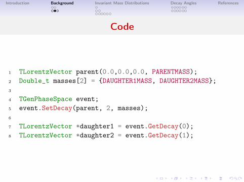
1 TLorentzVector parent(0.0,0.0,0.0, PARENTMASS);2 Double_t masses[2] = {DAUGHTER1MASS, DAUGHTER2MASS};3
4 TGenPhaseSpace event;5 event.SetDecay(parent, 2, masses);6
7 TLorentzVector *daughter1 = event.GetDecay(0);8 TLorentzVector *daughter2 = event.GetDecay(1);

Introduction Background Invariant Mass Distributions Decay Angles References
Code
This example code demonstrates the basic method; once you startlooking at longer decay chains and relativistically boosting andanalyzing them, it gets a lot more complicated! (And uglier...)
Introduction Background Invariant Mass Distributions Decay Angles References
Invariant Mass Distributions
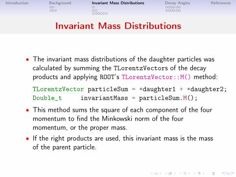
● The invariant mass distributions of the daughter particles wascalculated by summing the TLorentzVectors of the decayproducts and applying ROOT’s TLorentzVector::M() method:
TLorentzVector particleSum = *daughter1 + *daughter2;Double_t invariantMass = particleSum.M();
● This method sums the square of each component of the fourmomentum to find the Minkowski norm of the fourmomentum, or the proper mass.
● If the right products are used, this invariant mass is the massof the parent particle.

Introduction Background Invariant Mass Distributions Decay Angles References
Invariant Mass Distributions
The equations determining this in natural units (c = 1) are:
P =
⎛
⎜⎜⎜
⎝
P0
P1
P2
P3
⎞
⎟⎟⎟
⎠
=
⎛
⎜⎜⎜
⎝
Epxpypz
⎞
⎟⎟⎟
⎠
(1)
∥P∥2 = PµPµ = PµηµνPν = E 2− ∣p∣2 = m2 (2)
where ηµν is the Minkowski metric, here defined as:
ηµν =
⎛
⎜⎜⎜
⎝
1 0 0 00 −1 0 00 0 −1 00 0 0 −1
⎞
⎟⎟⎟
⎠
(3)

Introduction Background Invariant Mass Distributions Decay Angles References
Two body ψ(3770)→ D0D0
Invariant mass distribution of the D0 and D0 matches exactly withthe mass of the parent particle:
]2
) [GeV/c0
D0
m(D
3 3.1 3.2 3.3 3.4 3.5 3.6 3.7 3.8 3.9 40
20
40
60
80
100
310×
(3770) Meson Decayψ(3770) Meson Decayψ
Entries 100000
Mean 3.77
RMS 4.948e06
(3770) Meson Decayψ
Introduction Background Invariant Mass Distributions Decay Angles References
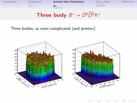
Three body B+→ D0D0K+
Three bodies, so more complicated (and prettier):
]2)2
) [(GeV/c
+K0
(D2m5
67
89
1011
12
]2)
2
) [(GeV/c
+K0D(
2m
56
78
910
1112
0
5
10
15
20
25
30
35
]2)2
) [(GeV/c
0D0
(D2m
1214
1618
2022
24
]2)
2
) [(GeV/c
+K0(D
2m
56
78
910
1112
0
10
20
30
40
50
60

Introduction Background Invariant Mass Distributions Decay Angles References
Three body B+→ D0D0K+
● A three body decay has a two-dimensional phase space, so thisis best visualised as a density plot of the invariant massdistributions of combinations of two of the particles.
● They are not unique and can be inferred from one another dueto momentum conservation laws.
● If there were no intermediate resonances in the decay, thisshould decay roughly uniformly throughout the phase space,meaning given if this MC were repeated an infinite number oftimes, the distribution would be approximately flat-topped.Considering the finite number of iterations made, this isn’tbad!
● An example of an intermediate resonance in this decay that weare very interested in is B → ψ(3770)K , which is notsimulated here but which we will look at later.

Introduction Background Invariant Mass Distributions Decay Angles References
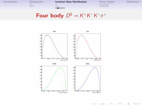
Four body D0→ K+K−K−π+
● Also looked at phase space for uniform four body decays.● These produce five dimensional phase space, which is hard tovisualise. I’ve just projected these onto axes to turn them into1D projections which can easily be plotted and understood.
● (If you want to know more about visualising multi-dimensionalphase spaces, talk to Dan Saunders.)
Introduction Background Invariant Mass Distributions Decay Angles References
Four body D0→ K+K−K−π+
]2 m(K K) [GeV/c1 1.05 1.1 1.15 1.2 1.25
0
50
100
150
200
250
300
350
400
K KK K
]2) [GeV/cπ m(K 0.65 0.7 0.75 0.8 0.85 0.9
0
50
100
150
200
250
300
350
400
πK πK
]2 m(K K K) [GeV/c1.5 1.55 1.6 1.65 1.7
0
50
100
150
200
250
300
350
400
K K KK K K
]2) [GeV/cπ m(K K 1.15 1.2 1.25 1.3 1.35
0
50
100
150
200
250
300
350
400
πK K πK K

Introduction Background Invariant Mass Distributions Decay Angles References
Four body D0→ K+K−K−π+
● If I had simulated intermediate resonances in the decay wewould see rich strong phase information arising from theinterference between these decays.
● If you’re interested in this, the structure of such decays using“Dalitz Plot Analysis” has been done by Bristol’s particlephysics team for D0
→ KKππ deacys, and Jack Benton is nowdoing a Dalitz plot analysis of D → ππππ decays.
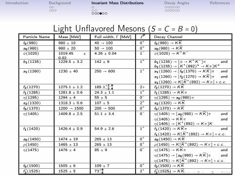
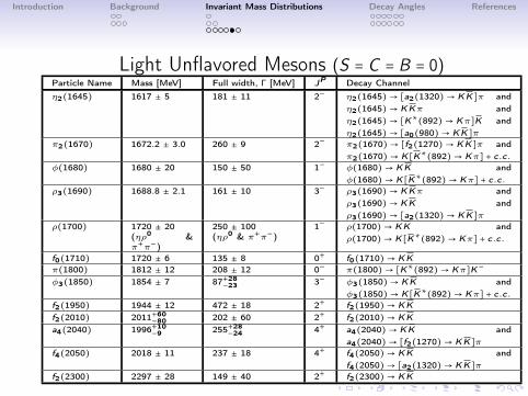
● The D0→ K+K−K−π+ decay strong phase information has
never been observed! For interest, I tabulated the possibleintermediate resonances:
Introduction Background Invariant Mass Distributions Decay Angles References
Light Unflavored Mesons (S = C = B = 0)Particle Name Mass [MeV] Full width, Γ [MeV] JP Decay Channelf0(980) 980 ± 10 40 → 100 0+ f0(980)→ KKa0(980) 980 ± 20 50 → 100 0+ a0(980)→ KKφ(1020) 1019.45 ±
0.024.26 ± 0.04 1− φ(1020)→ K+K−
b1(1235) 1229.5 ± 3.2 142 ± 9 1+ b1(1235)→ [φ→ K+K−]π and
b1(1235)→ [K∗(892)± → Kπ]K±
a1(1260) 1230 ± 40 250 → 600 1+ a1(1260)→ [f0(1370)→ KK]π anda1(1260)→ [f2(1270)→ KK]π anda1(1260)→ K[K∗
(892)→ Kπ] + c.c.f2(1270) 1275.1 ± 1.2 185.1+2.9
−2.4 2+ f2(1270)→ KKf1(1285) 1281.8 ± 0.6 24.3 ± 1.1 1+ f1(1285)→ KKπη(1295) 1294 ± 4 55 ± 5 0− η(1295)→ a0(980)πa2(1320) 1318.3 ± 0.6 107 ± 5 2+ a2(1320)→ KKf0(1370) 1200 → 1500 200 → 500 0+ f0(1370)→ KKη(1405) 1409.8 ± 2.5 51.1 ± 3.4 0− η(1405)→ [a0(980)→ KK]π and
η(1405)→ KKπ andη(1405)→ [K∗
(892)→ Kπ]Kf1(1420) 1426.4 ± 0.9 54.9 ± 2.6 1+ f1(1420)→ KKπ and
f1(1420)→ K[K∗(892)→ Kπ] + c.c.
a0(1450) 1474 ± 19 265 ± 13 0+ a0(1450)→ KKρ(1450) 1465 ± 13 265 ± 13 0+ ρ(1450)→ K[K∗
(892)→ Kπ] + c.c.η(1475) 1476 ± 4 85 ± 9 0− η(1475)→ KKπ and
η(1475)→ [a0(980)→ KK]π andη(1475)→ K[K∗
(892)→ Kπ] + c.c.f0(1500) 1505 ± 6 109 ± 7 0+ f0(1500)→ KKf ′2(1525) 1525 ± 5 73+6
−5 2+ f ′2(1525)→ KK
Introduction Background Invariant Mass Distributions Decay Angles References
Light Unflavored Mesons (S = C = B = 0)Particle Name Mass [MeV] Full width, Γ [MeV] JP Decay Channelη2(1645) 1617 ± 5 181 ± 11 2− η2(1645)→ [a2(1320)→ KK]π and
η2(1645)→ KKπ andη2(1645)→ [K∗
(892)→ Kπ]K andη2(1645)→ [a0(980)→ KK]π
π2(1670) 1672.2 ± 3.0 260 ± 9 2− π2(1670)→ [f2(1270)→ KK]π andπ2(1670)→ K[K∗
(892)→ Kπ] + c.c.φ(1680) 1680 ± 20 150 ± 50 1− φ(1680)→ KK and
φ(1680)→ K[K∗(892)→ Kπ] + c.c.
ρ3(1690) 1688.8 ± 2.1 161 ± 10 3− ρ3(1690)→ KKπ andρ3(1690)→ KK andρ3(1690)→ [a2(1320)→ KK]π
ρ(1700) 1720 ± 20(ηρ0 &π+π−)
250 ± 100(ηρ0 & π+π−)
1− ρ(1700)→ KK andρ(1700)→ K[K∗
(892)→ Kπ] + c.c.
f0(1710) 1720 ± 6 135 ± 8 0+ f0(1710)→ KKπ(1800) 1812 ± 12 208 ± 12 0− π(1800)→ [K∗
(892)→ Kπ]K−
φ3(1850) 1854 ± 7 87+28−23 3− φ3(1850)→ KK and
φ3(1850)→ K[K∗(892)→ Kπ] + c.c.
f2(1950) 1944 ± 12 472 ± 18 2+ f2(1950)→ KKf2(2010) 2011+60
−80 202 ± 60 2+ f2(2010)→ KKa4(2040) 1996+10
−9 255+28−24 4+ a4(2040)→ KK and
a4(2040)→ [f2(1270)→ KK]π
f4(2050) 2018 ± 11 237 ± 18 4+ f4(2050)→ KK andf4(2050)→ [a2(1320)→ KK]π
f2(2300) 2297 ± 28 149 ± 40 2+ f2(2300)→ KK

Introduction Background Invariant Mass Distributions Decay Angles References
Strange Mesons (S = ±1,C = B = 0)Particle Name Mass [MeV] Full width, Γ [MeV] JP Decay ChannelK∗
(892) 895.5 ± 0.8 46.2 ± 1.3 1−
K∗(892)→ KπK∗
(892)± 891.66 ± 0.26 50.8 ± 0.9 1−
K∗(892)0 895.94 ± 0.22 48.7 ± 0.8 1−
K1(1270) 1272 ± 7 90 ± 20 1+ K1(1270)→ K[f0(1370)→ KK]
K1(1400) 1403 ± 7 174 ± 13 1+ K1(1400)→ K[f0(1370)→ KK]
K∗(1410) 1414 ± 15 232 ± 21 1− K∗
(1410)→ KπK∗
0 (1430) 1425 ± 50 270 ± 80 0+ K∗
0 (1430)→ KπK∗
2 (1430)± 1425.6 ± 1.5 98.5 ± 2.7 2+ K∗
2 (1430)→ KπK∗
2 (1430)0 1432.4 ± 1.3 109 ± 5 2+
K∗(1680) 1717 ± 27 322 ± 110 1− K∗
(1680)→ KπK2(1770) 1773 ± 8 186 ± 14 2− K2(1770)→ K[f2(1270→ KK] and
K2(1770)→ K[φ→ K+K−]
K∗
3 (1780) 1776 ± 7 159 ± 21 3− K∗
3 (1780)→ KπK2(1820) 1816 ± 13 276 ± 35 2− K2(1820)→ K[f2(1270)→ KK]
K∗
4 (2045) 1045 ± 9 198 ± 30 4+ K∗
4 (2045)→ Kπ
Introduction Background Invariant Mass Distributions Decay Angles References
Decay Angles
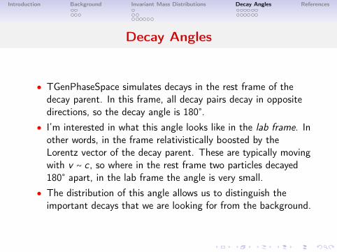
● TGenPhaseSpace simulates decays in the rest frame of thedecay parent. In this frame, all decay pairs decay in oppositedirections, so the decay angle is 180°.
● I’m interested in what this angle looks like in the lab frame. Inother words, in the frame relativistically boosted by theLorentz vector of the decay parent. These are typically movingwith v ∼ c , so where in the rest frame two particles decayed180° apart, in the lab frame the angle is very small.
● The distribution of this angle allows us to distinguish theimportant decays that we are looking for from the background.

Introduction Background Invariant Mass Distributions Decay Angles References
Decay Angles
Daughter 1
Daughter 2
α = 180° Daughter 1
Daughter 2
v ∼ c α ≃ 0 − 5°v = 0
Parent
Parent
Rest Frame Lab Frame
Introduction Background Invariant Mass Distributions Decay Angles References
ψ(3770)→ D0D0
● Before the decay angle in the lab frame can be calculated, firstyou need the Lorentz vector of the parent ψ(3770).
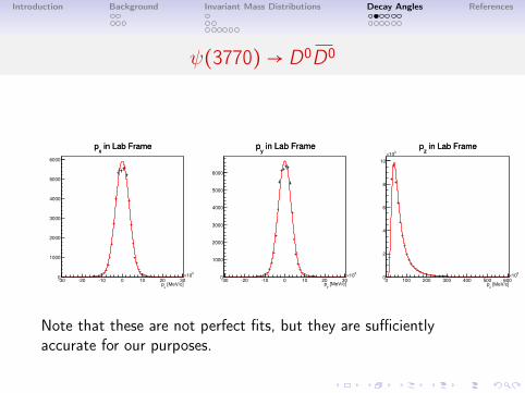
● To this end, momentum component distributions wereobtained from a LHCb Monte Carlo simulation.
● These momentum component distributions were fitted tomathematical functions.
● The MC simulation of the ψ(3770)→ D0D0 decay was thenrepeated a large number of times and each time the products’4-momenta were boosted by a random vector fitting themomentum distributions from the mathematical fit to the MCsimulation.
Introduction Background Invariant Mass Distributions Decay Angles References
ψ(3770)→ D0D0
[MeV/c]x
p30 20 10 0 10 20 30
310×0
1000
2000
3000
4000
5000
6000
in Lab Framex
p in Lab Framex
p
[MeV/c]y
p30 20 10 0 10 20 30
310×0
1000
2000
3000
4000
5000
6000
in Lab Framey
p in Lab Framey
p
[MeV/c]z
p0 100 200 300 400 500 600
310×0
2
4
6
8
10
310×
in Lab Framez
p in Lab Framez
p
Note that these are not perfect fits, but they are sufficientlyaccurate for our purposes.

Introduction Background Invariant Mass Distributions Decay Angles References
ψ(3770)→ D0D0
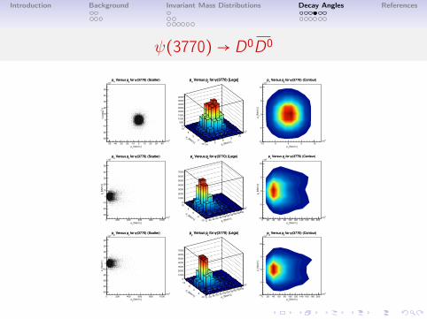
● Need to confirm independence of px , py and pz in order to usethem independently for TGenPhaseSpace simulation.
● Correlation factors between components calculated andtabulated:
px py pzpx 1 0.00640212 0.0150375py 0.00640212 1 0.0167604pz 0.0150375 0.0167604 1
● Following plots visualise this independence:
Introduction Background Invariant Mass Distributions Decay Angles References
ψ(3770)→ D0D0
[MeV/c]x
p
50 40 30 20 10 0 10 20 30 40
310×
[MeV
/c]
y p
30
20
10
0
10
20
30
40
50
310×
(3770) (Scatter)ψ for y
Versus px
p (3770) (Scatter)ψ for y
Versus px
p
[MeV/c]
x p105
05
10
310×
[MeV/c]
y
p
10
5
0
5
10
0
500
1000
1500
2000
2500
3000
3500
4000
(3770) [Lego]ψ for y
Versus px
p (3770) [Lego]ψ for y
Versus px
p
[MeV/c]x
p
10 5 0 5 10
310×
[M
eV
/c]
y p
10
5
0
5
10
310×
(3770) (Contour)ψ for y
Versus px
p (3770) (Contour)ψ for y
Versus px
p
[MeV/c]x
p
0 200 400 600 800 1000
310×
[M
eV
/c]
z p
30
20
10
0
10
20
30
40
50
310×
(3770) (Scatter)ψ for z
Versus px
p (3770) (Scatter)ψ for z
Versus px
p
[MeV/c]
x p0 20 40 60 80100120140160180200
310×
[MeV/c]
z
p
10
5
0
5
10
0
1000
2000
3000
4000
5000
6000
7000
(3770) (Lego)ψ for z
Versus px
p (3770) (Lego)ψ for z
Versus px
p
[MeV/c]x
p
0 20 40 60 80 100 120 140 160 180 200
310×
[M
eV
/c]
z p
10
5
0
5
10
310×
(3770) (Contour)ψ for z
Versus px
p (3770) (Contour)ψ for z
Versus px
p
[MeV/c]y
p
0 200 400 600 800 1000
310×
[M
eV
/c]
z p
50
40
30
20
10
0
10
20
30
40
310×
(3770) (Scatter)ψ for z
Versus py
p (3770) (Scatter)ψ for z
Versus py
p
[MeV/c]
y p0 20 40 60 80100120140160180200
310×
[MeV/c]
z
p
10
5
0
5
10
0
1000
2000
3000
4000
5000
6000
7000
(3770) (Lego)ψ for z
Versus py
p (3770) (Lego)ψ for z
Versus py
p
[MeV/c]y
p
0 20 40 60 80 100 120 140 160 180 200
310×
[M
eV
/c]
z p
10
5
0
5
10
310×
(3770) (Contour)ψ for z
Versus py
p (3770) (Contour)ψ for z
Versus py
p
Introduction Background Invariant Mass Distributions Decay Angles References
ψ(3770)→ D0D0
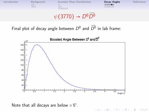
Final plot of decay angle between D0 and D0 in lab frame:
]° Angle [ 0 0.5 1 1.5 2 2.5 3 3.5 4 4.5 5
0
20
40
60
80
100
120
140
160
180
310×
0D and 0Boosted Angle Between D
0D and 0Boosted Angle Between D
Note that all decays are below ≃ 5°.

Introduction Background Invariant Mass Distributions Decay Angles References
ψ(3770)→ D0D0
● Importance of this graph is that the decay angle is highlypeaked around ∼ 0.5°
● This makes it very useful for distinguishing this interestingdecay channel from the uninteresting background, whichshould not be peaked but more evenly angularly distributed(although it may have some angular dependence).
Introduction Background Invariant Mass Distributions Decay Angles References
B → (ψ(3770)→ D0D0)K
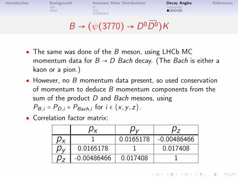
● The same was done of the B meson, using LHCb MCmomentum data for B → D Bach decay. (The Bach is either akaon or a pion.)
● However, no B momentum data present, so used conservationof momentum to deduce B momentum components from thesum of the product D and Bach mesons, usingPB,i = PD,i + PBach,i for i ∈ {x , y , z}.
● Correlation factor matrix:
px py pzpx 1 0.0165178 -0.00486466py 0.0165178 1 0.017408pz -0.00486466 0.017408 1

Introduction Background Invariant Mass Distributions Decay Angles References
B → (ψ(3770)→ D0D0)K
(MeV/c)y
p30 20 10 0 10 20 30 40
310×
x p
50
40
30
20
10
0
10
20
30
40
310×
for B (Scatter)y
Versus px
p for B (Scatter)y
Versus px
p
(MeV/c)
y p
30 2010 0
10 20 3040
310×x
p
5040
3020
100
1020
3040
0
20
40
60
80
100
for B (Lego)y
Versus px
p for B (Lego)y
Versus px
p
(MeV/c)y
p30 20 10 0 10 20 30 40
310×
x p
50
40
30
20
10
0
10
20
30
40
310×
for B (Contour)y
Versus px
p for B (Contour)y
Versus px
p
(MeV/c)z
p0 0.2 0.4 0.6 0.8 1
610×
x p
50
40
30
20
10
0
10
20
30
40
310×
for B (Scatter)z
Versus px
p for B (Scatter)z
Versus px
p
(MeV/c)
z p
00.2
0.40.6
0.81
610×x
p
5040
3020
100
1020
3040
0
20
40
60
80
100
120
140
160
180
200
for B (Lego)z
Versus px
p for B (Lego)z
Versus px
p
(MeV/c)z
p0 0.2 0.4 0.6 0.8 1
610×
x p
50
40
30
20
10
0
10
20
30
40
310×
for B (Contour)z
Versus px
p for B (Contour)z
Versus px
p
(MeV/c)z
p0 0.2 0.4 0.6 0.8 1
610×
y p
30
20
10
0
10
20
30
40
310×
for B (Scatter)z
Versus py
p for B (Scatter)z
Versus py
p
(MeV/c)
z p
00.2
0.40.6
0.81
610×y
p
3020
100
1020
3040
0
20
40
60
80
100
120
140
160
for B (Lego)z
Versus py
p for B (Lego)z
Versus py
p
(MeV/c)z
p0 0.2 0.4 0.6 0.8 1
610×
y p
30
20
10
0
10
20
30
40
310×
for B (Contour)z
Versus py
p for B (Contour)z
Versus py
p

Introduction Background Invariant Mass Distributions Decay Angles References
B → (ψ(3770)→ D0D0)K
(MeV/c)x
p50 40 30 20 10 0 10 20 30 40
310×0
50
100
150
200
250
300
350
400
450
500x
B Meson px
B Meson p
(MeV/c)y
p30 20 10 0 10 20 30 40
310×0
50
100
150
200
250
300
350
400y
B Meson py
B Meson p
(MeV/c)z
p0 0.2 0.4 0.6 0.8 1
610×0
100
200
300
400
500
600
700
zB Meson p
zB Meson p

Introduction Background Invariant Mass Distributions Decay Angles References
B → (ψ(3770)→ D0D0)K
Final decay angle graphs:
In rest frame of parent B :
]° Angle [ 179 179.2179.4179.6179.8 180 180.2180.4180.6180.8 1810
2
4
6
8
10
610×
(3770) and KψNonBoosted Angle Between (3770) and KψNonBoosted Angle Between
]° Angle [ 0 10 20 30 40 50
0
0.5
1
1.5
2
2.5
610×
0D and
0NonBoosted Angle Between D
0D and
0NonBoosted Angle Between D
Introduction Background Invariant Mass Distributions Decay Angles References
B → (ψ(3770)→ D0D0)K
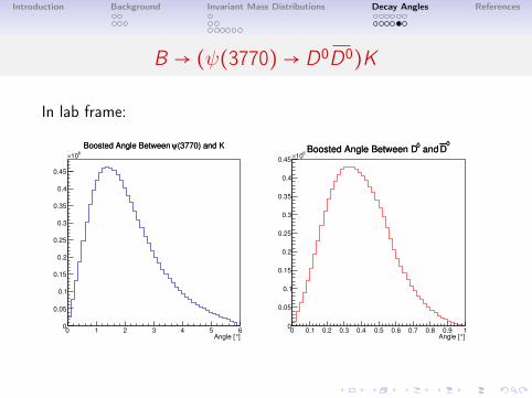
In lab frame:
]° Angle [ 0 1 2 3 4 5 6
0
0.05
0.1
0.15
0.2
0.25
0.3
0.35
0.4
0.45
610×
(3770) and KψBoosted Angle Between (3770) and KψBoosted Angle Between
]° Angle [ 0 0.1 0.2 0.3 0.4 0.5 0.6 0.7 0.8 0.9 1
0
0.05
0.1
0.15
0.2
0.25
0.3
0.35
0.4
0.456
10×
0D and
0Boosted Angle Between D
0D and
0Boosted Angle Between D

Introduction Background Invariant Mass Distributions Decay Angles References
B → (ψ(3770)→ D0D0)K
● Once again, we find that the decay angle is sharply peakedaround ≃ 1.5° for the ψ(3770) −K angle and ≃ 0.4° for theD0
−D0 angle.● This is good, because it means that the decay angle canaccurately be used to distinguish this interesting decay from allthe uninteresting background decays going on.
● This allows us to isolate more ψ(3770) decays for symmetryviolation studies.

Introduction Background Invariant Mass Distributions Decay Angles References
References
● http://root.cern.ch/root/html/TGenPhaseSpace.html
● http://cds.cern.ch/record/275743


