Abstract In this paper, we present a particle swarm optimizer (PSO) to solve the variableweighting problem in projected clustering of high-dimensional data. Many subspace clus-tering algorithms fail to yield good cluster quality because they do not employ an efficientsearch strategy. In this paper, we are interested in soft projected clustering. We design asuitable k-means objective weighting function, in which a change of variable weights isexponentially reflected. We also transform the original constrained variable weighting prob-lem into a problem with bound constraints, using a normalized representation of variableweights, and we utilize a particle swarm optimizer to minimize the objective function inorder to search for global optima to the variable weighting problem in clustering. Our ex-perimental results on both synthetic and real data show that the proposed algorithm greatlyimproves cluster quality. In addition, the results of the new algorithm are much less depen-dent on the initial cluster centroids. In an application to text clustering, we show that thealgorithm can be easily adapted to other similarity measures, such as the extended Jaccardcoefficient for text data, and can be very effective.
Keywords High-dimensional data · Projected clustering · Variable weighting · Particleswarm optimization · Text clustering
1 Introduction
Clustering high-dimensional data is a common task in various data mining applications.Text clustering is a typical example. In text mining, a text dataset is viewed as a matrix,
Editors: D. Martens, B. Baesens, and T. Fawcett.
Y. Lu (�) · S. WangDepartment of Computer Science, University of Sherbrooke, 2500 Boul. de l’Universite, Sherbrooke,Quebec, J1K 2R1, Canadae-mail: [email protected]
Y. Lu · S. Li · C. ZhouDepartment of Cognitive Science, Xiamen University, Xiamen, 361005, China
where a row represents a document and a column represents a unique term. The number ofdimensions is represented by the number of unique terms, which is usually in the thousands.Another application where high-dimensional data occurs is insurance company customerprediction. It is important to separate customers into groups to help companies predict whowould be interested in buying an insurance policy (van der Putten and Someren 2000). Manyother applications, such as bankruptcy prediction, web mining, protein function prediction,etc., present similar data analysis problems.
Clustering high-dimensional data is a difficult task because clusters of high-dimensionaldata are usually embedded in lower-dimensional subspaces. Traditional clustering algo-rithms struggle with high-dimensional data because the quality of results deteriorates dueto the curse of dimensionality. As the number of dimensions increases, data becomes verysparse and distance measures in the whole dimension space become meaningless. In fact,some dimensions may be irrelevant or redundant for clusters and different sets of dimen-sions may be relevant for different clusters. Thus, clusters should often be searched for insubspaces of dimensions rather than the whole dimension space.
According to the definition of the problem, the approaches to identify clusters on suchdatasets are categorized into three types (Kriegel et al. 2009). The first, subspace clustering,aims to identify clusters in all subspaces of the entire feature space (see for instance Agrawalet al. 2005; Goil et al. 1999; Moise and Sander 2008). The second, projected clustering,aims to partition the dataset into disjoint clusters (see for instance Procopiuc et al. 2002;Woo et al. 2004). The third type, hybrid clustering, includes algorithms that fall into neitherof the first two types (see for instance Elke et al. 2008; Moise et al. 2008). The performanceof many subspace/projected clustering algorithms drops quickly with the size of the sub-spaces in which the clusters are found (Parsons et al. 2004). Also, many of them requiredomain knowledge provided by the user to help select and tune their settings, such as themaximum distance between dimensional values (Procopiuc et al. 2002), the threshold of in-put parameters (Elke et al. 2008; Moise et al. 2008) and the density (Agrawal et al. 2005;Goil et al. 1999; Moise and Sander 2008), which are difficult to set.
Recently, soft projected clustering, a special case of projected clustering, has been de-veloped to identify clusters by assigning an optimal variable weight vector to each cluster(Domeniconi et al. 2007; Huang et al. 2005; Jing et al. 2007). Each of these algorithms min-imizes a k-means like objective function iteratively. Although the cluster membership of anobject is calculated in the whole variable space, the similarity between each pair of objectsis based on weighted variable differences. The variable weights transform the Euclidean dis-tance used in conventional k-means algorithm so that the associated cluster is reshaped intoa dense hypersphere and can be separated from other clusters. Soft projected clustering al-gorithms are driven by evaluation criteria and search strategies. Consequently, how to definethe objective function and how to efficiently determine the optimal variable weighting arethe two most important issues in soft projected clustering.
In this paper, we propose a particle swarm optimizer to obtain optimal variable weights insoft projected clustering of high-dimensional data. Good clustering quality is very dependenton a suitable objective function and an efficient search strategy. Our new soft projected clus-tering algorithm employs a special k-means objective weighting function, which takes thesum of the within-cluster distances of each cluster along relevant dimensions preferentiallyto irrelevant ones. If a variable is considered insignificant and assigned a small weight, thecorresponding distance along this dimension will thus tend to be zero because the weightsare handled exponentially. As a result, the function is more sensitive to changes in variableweights. In order to precisely measure the contribution of each dimension to each cluster,we assign a weight to each dimension in each cluster, following Domeniconi et al. (2007),Jing et al. (2007).
Mach Learn (2011) 82: 43–70 45
The new algorithm also utilizes a normalized representation of variable weights in theobjective function and transforms the constrained search space for the variable weightingproblem in soft projected clustering into a redundant closed space, which greatly facilitatesthe search process. Instead of employing local search strategies, the new algorithm makesfull use of a particle swarm optimizer to minimize the given objective function. It is simpleto implement and the results are much less sensitive to the initial cluster centroids thanthose of other soft projected clustering algorithms. Experimental results on both syntheticdatasets from a data generator and real datasets from the UCI database show that it cangreatly improve cluster quality.
The rest of the paper is organized as follows. Section 2 reviews some previous relatedwork on the variable weighting problem in soft projected clustering, explains the rationalebehind using PSO for this problem and introduces the principle of PSO. Section 3 utilizes aparticle swarm optimizer to assign the optimal variable weight vector for each cluster in softprojected clustering. Simulations on synthetic data are given in Section 4, which contains thedescription of synthetic datasets with different characteristics, the experimental setting forthe PSO, and experimental results. In Section 5, experimental results on three real datasetsare presented. An application of our new soft projected clustering algorithm to handle theproblem of text clustering is given in Section 6. Section 7 draws conclusions and givesdirections for future work.
2 Previous work
2.1 Soft projected clustering
Assuming that the number of clusters k is given and that all of the variables for the datasetsare comparable, soft projected clustering algorithms (Domeniconi et al. 2007; Huang et al.2005; Jing et al. 2007) have been designed to discover clusters in the full dimensional space,by assigning a weight to each dimension for each cluster. The variable weighting problemis an important issue in data mining (Makarenkov and Legendre 2001). Usually, variablesthat correlate strongly with a cluster obtain large weights, which mean that these variablescontribute strongly to the identification of data objects in the cluster. Irrelevant variables ina cluster obtain small weights. Thus, the computation of the membership of a data objectin a cluster depends on the variable weights and the cluster centroids. The most relevantvariables for each cluster can often be identified by the weights after clustering.
The performance of soft projected clustering largely depends on the use of a suitableobjective function and an efficient search strategy. The objective function determines thequality of the partitioning, and the search strategy has an impact on whether the optimumof the objective function can be reached. Recently, several soft projected clustering algo-rithms have been proposed to perform the task of projected clustering and to select relevantvariables for clustering.
Domeniconi et al. proposed the LAC algorithm, which determines the clusters by mini-mizing the following objective function (Domeniconi et al. 2007):
F(w) =k∑
l=1
m∑
j=1
(wl,j · Xl,j + h · wl,j · logwl,j ), Xl,j =∑n
i=1 ui,l · (xi,j − zl,j )2
∑n
i=1 ui,l
, (1)
s.t.
{∑m
j=1 wl,j = 1, 0 ≤ wl,j ≤ 1, 1 ≤ l ≤ k,
∑k
l=1 ui,l = 1, ui,l ∈ {0,1}, 1 ≤ i ≤ n,(2)
46 Mach Learn (2011) 82: 43–70
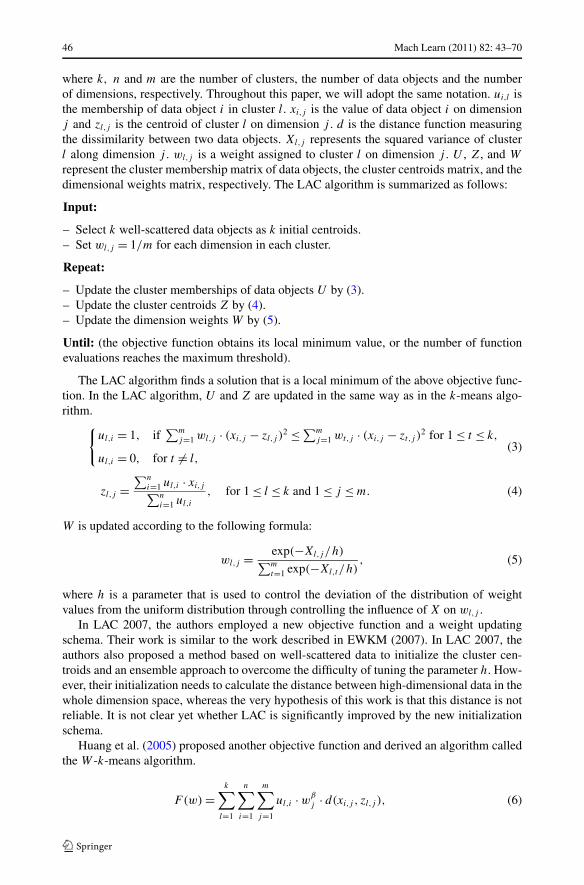
where k, n and m are the number of clusters, the number of data objects and the numberof dimensions, respectively. Throughout this paper, we will adopt the same notation. ui,l isthe membership of data object i in cluster l. xi,j is the value of data object i on dimensionj and zl,j is the centroid of cluster l on dimension j . d is the distance function measuringthe dissimilarity between two data objects. Xl,j represents the squared variance of clusterl along dimension j . wl,j is a weight assigned to cluster l on dimension j . U , Z, and W
represent the cluster membership matrix of data objects, the cluster centroids matrix, and thedimensional weights matrix, respectively. The LAC algorithm is summarized as follows:
Input:
– Select k well-scattered data objects as k initial centroids.– Set wl,j = 1/m for each dimension in each cluster.
Repeat:
– Update the cluster memberships of data objects U by (3).– Update the cluster centroids Z by (4).– Update the dimension weights W by (5).
Until: (the objective function obtains its local minimum value, or the number of functionevaluations reaches the maximum threshold).
The LAC algorithm finds a solution that is a local minimum of the above objective func-tion. In the LAC algorithm, U and Z are updated in the same way as in the k-means algo-rithm.
{ul,i = 1, if
∑m
j=1 wl,j · (xi,j − zl,j )2 ≤ ∑m
j=1 wt,j · (xi,j − zt,j )2 for 1 ≤ t ≤ k,
ul,i = 0, for t �= l,(3)
zl,j =∑n
i=1 ul,i · xi,j∑n
i=1 ul,i
, for 1 ≤ l ≤ k and 1 ≤ j ≤ m. (4)
W is updated according to the following formula:
wl,j = exp(−Xl,j /h)∑m
t=1 exp(−Xl,t /h), (5)
where h is a parameter that is used to control the deviation of the distribution of weightvalues from the uniform distribution through controlling the influence of X on wl,j .
In LAC 2007, the authors employed a new objective function and a weight updatingschema. Their work is similar to the work described in EWKM (2007). In LAC 2007, theauthors also proposed a method based on well-scattered data to initialize the cluster cen-troids and an ensemble approach to overcome the difficulty of tuning the parameter h. How-ever, their initialization needs to calculate the distance between high-dimensional data in thewhole dimension space, whereas the very hypothesis of this work is that this distance is notreliable. It is not clear yet whether LAC is significantly improved by the new initializationschema.
Huang et al. (2005) proposed another objective function and derived an algorithm calledthe W -k-means algorithm.
F(w) =k∑
l=1
n∑
i=1
m∑
j=1
ul,i · wβ
j · d(xi,j , zl,j ), (6)
Mach Learn (2011) 82: 43–70 47
s.t.
{∑m
j=1 wj = 1, 0 ≤ wj ≤ 1, 1 ≤ l ≤ k,
∑k
l=1 ui,l = 1, ui,l ∈ {0,1}, 1 ≤ i ≤ n.(7)
Here, β is a parameter greater than 1. The objective function is designed to measure the sumof the within-cluster distances along variable subspaces rather than over the entire variable(dimension) space. The variable weights in the W -k-means need to meet the equality con-straints, which are similar to those of (2) in LAC. The formula for updating the weights isdifferent and is written as follows:
wj =⎧⎨
⎩
0, if Dj = 0,
1∑m
t=1[ DjDt
]1/(β−1), Dj = ∑k
l=1
∑n
i=1 ui,l · d(xi,j , zl,j ),(8)
where the weight wj for the j -th dimension is inversely proportional to the sum of all thewithin-cluster distances along dimension j . A large weight value corresponds to a small sumof within-cluster distances in a dimension, indicating that the dimension is more importantin forming the clusters.
The W -k-means algorithm is a direct extension of the k-means algorithm. The W -k-means assigns a weight to each variable and seeks to minimize the sum of all the within-cluster distances in the same subset of variables. Furthermore, updating of variable weightsis dependent on the value of the parameter β . In addition, the W -k-means algorithm doesnot utilize an efficient search strategy. Consequently, it has difficulty to correctly discoverclusters embedded in different subsets of variables. Because it assigns a unique weight toeach variable for all the clusters, the W -k-means algorithm is not appropriate in the mostcases of high-dimensional data where each cluster has its own relevant subset of variables.
To improve the W -k-means algorithm, Jing et al. (2007) proposed the entropy weightingk-means algorithm (EWKM), which assigns one weight to each variable for each cluster andemploys a similar iterative process to that used by the W -k-means algorithm. The objectivefunction in the EWKM algorithm takes both the within-cluster dispersion and the weightentropy into consideration. The function is described as follows:
F(w) =k∑
l=1
[n∑
i=1
m∑
j=1
ui,l · wl,j · (xi,j − zl,j )2 + γ ·
m∑
j=1
wl,j · logwl,j
], (9)
s.t.
{∑m
j=1 wl,j = 1, 0 ≤ wl,j ≤ 1, 1 ≤ l ≤ k,
∑k
l=1 ui,l = 1, ui,l ∈ {0,1}, 1 ≤ i ≤ n.(10)
The constraints in (10) of the above function are identical to those in the LAC algorithm.The formula for updating the weights is written as follows:
wl,j = exp(−Dl,j /γ )∑m
t=1 exp(−Dl,t /γ ), Dl,j =
n∑
i=1
ui,l · (xi,j − zl,j )2.
The objective (9) depends heavily on the value of parameter γ . If γ is too small, theentropy section has little effect on the function. On the other hand, if γ is too big, theentropy section could have too strong an effect on the function. The value of γ is empiricallydetermined and application-specific.
48 Mach Learn (2011) 82: 43–70
The computational complexity of LAC, the W -k-means and EWKM is O(mnkT ), whereT is the total number of iterations and m, n, k are the number of dimensions, the numberof data objects and the number of clusters, respectively. Their computational complexityis low and increases linearly as the number of dimensions, the number of data objects orthe number of clusters increases. Thus, these three principal algorithms for soft projectedclustering scale well with the data size. They can converge to a local minimal solution aftera finite number of iterations. However, since LAC, the W -k-means and EWKM all stem fromthe k-means algorithm, they share some common problems. First, the constrained objectivefunctions they provide have their drawbacks, which have been described above. Second, thecluster quality they yield is highly sensitive to the initial cluster centroids (see experiments).All the three algorithms employ local search strategies to optimize their objective functionswith constraints. The local search strategies provide good convergence speed to the iterativeprocess but do not guarantee good clustering quality because of local optimality.
2.2 Rationale for using PSO for the variable weighting problem
Basically, the variable weighting problem in soft projected clustering is a continuous non-linear optimization problem with many equality constraints. It is a difficult problem, andhas been researched for decades in the optimization field. Computational intelligence-basedtechniques, such as the genetic algorithm (GA), particle swarm optimization (PSO) and antcolony optimization (ACO), have been widely used to solve the problem.
GA is a heuristic search technique used in computing to find exact or approximate so-lutions to optimization problems. Genetic algorithms are a particular class of evolutionarycomputation that use techniques inspired by evolutionary biology, such as inheritance, mu-tation, selection, and crossover. In GA, the individuals of the population are usually repre-sented by candidate solutions to an optimization problem. The population starts from ran-domly generated individuals and evolves towards better solutions over generations. In eachgeneration, the fitness of every individual is evaluated; multiple individuals are selectedfrom the current population based on their fitness, and recombined and mutated to forma new population. The population iterates until the algorithm terminates, by which time asatisfactory solution may be reached.
ACO is a swarm intelligence technique introduced by Marco Dorigo in 1992. It is a prob-abilistic technique for solving computational problems which can be reduced to finding goodpaths through graphs. In ACO, ants initially wander randomly and, upon finding food, returnto the colony while laying down pheromone trails. Other ants follow the trail, returning andreinforcing it if they find food. However, the pheromone trail starts to evaporate over time,lest the paths found by the first ants should tend to be excessively attractive to the followingones. A short path gets marched over comparatively faster, and thus the pheromone densityremains high as it is laid on the path as fast as it can evaporate. Thus, when one ant finds agood (i.e., short) path from the colony to a food source, other ants are more likely to followthat path, and positive feedback eventually results in all the ants following a single path.
PSO is another swarm intelligence technique, first developed by James Kennedy andRussell C. Eberhart in 1995. It was inspired by the social behavior of bird flocking andfish schooling. PSO simulates social behavior. In PSO, each solution to a given problem isregarded as a particle in the search space. Each particle has a position (usually a solution tothe problem) and a velocity. The positions are evaluated by a user-defined fitness function.At each iteration, the velocities of the particles are adjusted according to the historical bestpositions of the population. The particles fly towards better regions through their own effortand in cooperation with other particles. Naturally, the population evolves to an optimal ornear-optimal solution.
Mach Learn (2011) 82: 43–70 49
PSO can generate a high-quality solution within an acceptable calculation time and a sta-ble convergence characteristic in many problems where most other methods fail to converge.It can thus be effectively applied to various optimization problems. A number of papers havebeen published in the past few years that focus on the applications of PSO, such as neuralnetwork training (Bergh and Engelbecht 2000), power and voltage control (Yoshida et al.2000), task assignment (Salman et al. 2003), single machine total weighted tardiness prob-lems (Tasgetiren et al. 2004) and automated drilling (Onwubolu and Clerc 2004). Moreover,PSO has some advantages over other similar computational intelligence-based techniquessuch as GA and ACO for solving the variable weighting problem for high-dimensional clus-tering. For instance:
(1) PSO is easier to implement and more computationally efficient than GA and ACO.There are fewer parameters to adjust. PSO only deals with two simple arithmetic oper-ations (addition and multiplication), while GA needs to handle more complex selectionand mutation operators.
(2) In PSO, every particle remembers its own historic best position, while every ant in ACOneeds to track down a series of its own previous positions and individuals in GA haveno memory at all. Therefore, a particle in PSO requires less time to calculate its fitnessvalue than an ant in ACO due to the simpler memory mechanism, while sharing thestrong memory capability of the ant at the same time. PSO has a more effective memorycapability than GA.
(3) PSO is more efficient in preserving population diversity to avoid the premature conver-gence problem. In PSO, all the particles improve themselves using their own previousbest positions and are improved by other particles’ previous best position by cooperat-ing with each other. In GA, there is “survival of the fittest”. The worst individuals arediscarded and only the good ones survive. ACO easily loses population diversity be-cause ants are attracted by the largest pheromone trail and there is no direct cooperationamong ants.
(4) PSO has been found to be robust, especially in solving continuous nonlinear optimiza-tion problems, while GA and ACO are good choices for constrained discrete optimiza-tion problems. ACO has an advantage over other evolutionary approaches when thegraph may change dynamically, and can be run continuously and adapt to changes inreal time.
Since the PSO method is an excellent optimization methodology for solving complexparameter estimation problems, we have developed a PSO-based algorithm for computingthe optimal variable weights in soft projected clustering.
2.3 PSO
In PSO, each solution is regarded as a particle in the search space. Each particle has aposition (usually a solution to the problem) and a velocity. The particles fly through thesearch space through their own effort and in cooperation with other particles.
The velocity and position updates of the ith particle are as follows:
where Xi is the position of the ith particle, Vi presents its velocity and pBesti is its personalbest position yielding the best function value for it. gBest is the global best position discov-ered by the whole swarm. λ is the inertia weight used to balance the global and local searchcapabilities. c1 and c2 are the acceleration constants, which represent the weights pullingeach particle toward the pbest and gbest positions, respectively. r1 and r2 are two randomnumbers uniformly distributed in the range [0,1].
The original PSO algorithm was later modified by the researchers in order to improve itsperformance. Comprehensive Learning Particle Swarm Optimizer (CLPSO), which is one ofthe well-known modifications of PSO, was proposed by Liang (2006) to efficiently optimizemultimodal functions. The following velocity update was employed in CLPSO:
where Cpbesti is a comprehensive learning result from the personal best positions of someparticles. CLPSO achieves good diversity and effectively solves the premature convergenceproblem in PSO. The CLPSO algorithm for a minimum optimization problem is summarizedas follows:
Initialization:
– Randomly initialize the position and velocity swarms, X and V .– Evaluate the fitness of X by the objective function.– Record the personal best position swarm pBest and the global best position gBest.
Repeat:
– Produce CpBest from pBest for each particle.– Update V and X by (13) and (12), respectively.– Update pBest and gBest.
Until: (the objective function reaches a global minimum value, or the number of functionevaluations reaches the maximum threshold).
3 PSO for variable weighting
In this section, we proposed a PSO-based algorithm, called PSOVW, to solve the variableweighting problem in soft projected clustering of high-dimensional data. We begin by show-ing how the problem of minimization of a special k-means function with equality constraintscan be transformed into a nonlinear optimization problem with bound constraints, using anormalized representation of variable weights in the objective function, and how a particleswarm optimizer can be used to control the search progress. We then give a detailed de-scription of our PSOVW algorithm, which minimizes the transformed problem. Finally, wediscuss the computational complexity of the proposed algorithm.
3.1 PSO for variable weighting (PSOVW)
Our particle swarm optimizer for the variable weighting problem in soft projected clustering,termed PSOVW, performs on two main swarms of variable weights, the position swarm W
and the personal best position swarm of variable weights pBest. The position swarm is the
Mach Learn (2011) 82: 43–70 51
foundation of the search in the variable weights space, so the evolution of the position swarmpays more attention to global search, while the personal best position swarm tracks the fittestpositions, in order to accelerate the convergence. In addition, it facilitates cooperation amongthe previous best positions in order to maintain the swarm diversity.
The objective function
We minimize the following objective function in PSOVW:
F(W) =k∑
l=1
n∑
i=1
m∑
j=1
ul,i ·(
wl,j∑m
j=1 wl,j
)β
· d(xi,j , zl,j ), (14)
s.t.
{0 ≤ wl,j ≤ 1,∑k
l=1 ui,l = 1, ui,l ∈ {0,1}, 1 ≤ i ≤ n.(15)
Actually, the objective function in (14) is a generalization of some existing objective func-tions. If β = 0, (14) is similar to the objective function used in the k-means. They differsolely in the representation of variable weights and the constraints. If β = 1, (14) is alsosimilar to the first section of the objective function in EWKM, differing only in the rep-resentation of variable weights and the constraints. If wl,j = wj , ∀l, (14) is similar to theobjective function in the W -k-means, which assigns a single variable weight vector, substi-tuting different vectors for clusters. Again, the difference is in the representation of variableweights and the constraints.
In PSOVW, β is a user-defined parameter. PSOVW works with all non-negative valuesof β . In practice, we suggest setting β to a large value (empirically around 8). A large valueof β makes the objective function more sensitive to changes in weight values. It tends tomagnify the influence of those variables with large weights on the within-cluster variance,allowing them to play a strong role in discriminating between relevant and irrelevant vari-ables (dimensions). On the other hand, in contrast to LAC and EWKM algorithms in whichthe variable weight matrix W is part of the solution to the objective function and must meetthe equality constraints, a normalized matrix W is employed in the objective function inPSOVW. Although the normalized representation in the constrained objective function (14)is redundant, the constraints can be loosened without affecting the final solution. As a result,the initialization and search processes only need to deal with bound constraints instead ofmany more complicated equality constraints. PSOVW includes three parts.
Initialization
In the PSOVW algorithm, we initialize three swarms.
– The position swarm W of variable weights are set to random numbers uniformly distrib-uted in a certain range R.
– The velocity swarm V of variable weights are set to random numbers uniformly distrib-uted in the range [−maxv,maxv]. Here, maxv means the maximum flying velocity ofparticles and maxv = 0.25 ∗ R.
– The swarm Z of cluster centroids are k different data objects randomly chosen out of allthe data objects.
In all three swarms, an individual is the k ∗ m matrix. Actually, only the velocity swarmV is an extra swarm not included in k-means-type soft projected clustering algorithms.
52 Mach Learn (2011) 82: 43–70
Update of cluster centroids and partitioning of data objects
Given the variable weight matrix and the cluster centroids, the cluster membership of eachdata object is calculated by the following formula.
⎧⎪⎪⎨
⎪⎪⎩
ul,i = 1, if∑m
j=1(wl,j∑m
j=1 wl,j)β · d(zl,j , xi,j ) ≤ ∑m
j=1(wq,j∑m
j=1 wq,j)β · d(zt,j , xi,j )
for 1 ≤ q ≤ k,
ul,i = 0, for q �= l.
(16)
Once the cluster membership is obtained, the cluster centroids are updated by
zl,j =(
n∑
i=1
ul,i · xi,j
)/(n∑
i=1
ul,i
), for 1 ≤ l ≤ k and 1 ≤ j ≤ m. (17)
In our implementation, if an empty cluster results from the membership update by for-mula (16), we randomly select a data object out of the dataset to reinitialize the centroidof the cluster.
Crossover learning
Given a value for β , two extra swarms are kept to guide all the particles’ movement inthe search space. One is the personal best position swarm of variable weights pBest, whichkeeps the best position of the weight matrix W ; i.e., pBest will be replaced by W if F(W) <
F(pBest). The other is the crossover best position swarm of variable weights CpBest, whichguides particles to move towards better regions (Liang et al. 2006). CpBest is obtained bya crossover operation between its own pBest and one of the other best personal positions inthe swarm, represented here by s_pBest.
The tournament mechanism is employed to select s_pBest, with the consideration thata particle learns from a good exemplar. First, two individuals, pBest1 and pBest2, are ran-domly selected. Then their objective function values are compared: s_pBest = pBest1 ifF(pBest1) < F(pBest2), s_pBest = pBest2 otherwise. The crossover is done as follows.Each element at a position of CpBest is assigned the value either from s_pBest or from pBestat the corresponding position. This assignment is made randomly according to a user-definedprobability value Pc (see the section Synthetic Data Simulations for further discussion). If,despite the random assignment process, all the elements of CpBest take values from its ownpBest, one element of CpBest will be randomly selected and its value will be replaced bythe value of the corresponding position from s_pBest.
The PSOVW algorithm can be summarized as follows:
Initialization:
– Randomly initialize the position swarm W in the range of [0,1] and the velocity swarmV in the range of [−mv,mv], where mv = 0.25 ∗ (1 − 0). Randomly select a set of k dataobjects out of the dataset as a set of k cluster centroids in the cluster centroid swarm.
– Partition the data objects by the formula (16).– For each position W ,
If W lies in the range [0,1],Evaluate the fitness function value F(W) of W by the formula (14).Record the swarm pBest and the best position gBest.
Mach Learn (2011) 82: 43–70 53
Otherwise,W is neglected.
End
Repeat:
– For each position W ,Produce CpBest from the swarm pBests.Update V and W by (13) and (12), respectively.If W lies in the range [0,1],
Evaluate its fitness by (14).Update the position’s pBest and gBest.
Otherwise,W is neglected.
End.
Until: (the objective function reaches a global minimum value, or the number of functionevaluations reaches the maximum threshold).
3.2 Computational complexity
The computational complexity can be analyzed as follows. In the PSOVW algorithm, theCpBest, position and velocity of a particle are k ∗ m matrices. In the main loop procedure,after initialization of the position and velocity, generating CpBest and updating position andvelocity need O(mk) operations for each particle. Given the weight matrix W and the clus-ter centroids matrix Z, the complexity for partitioning the data objects is O(mnk) for eachparticle. The complexity for updating cluster centers is O(mk) for each particle. Assumingthat the PSOVW algorithm needs T iterations to converge, the total computational complex-ity of the PSOVW algorithm is O(smnkT ). The swarm size s is usually a constant set by theuser. So, the computational complexity still increases linearly as the number of dimensions,the number of objects or the number of clusters increases.
4 Synthetic data simulations
A comprehensive performance study was conducted to evaluate the performance of PSOVWon high-dimensional synthetic datasets as well as on real datasets. Three of the most widelyused soft projected clustering algorithms, LAC (Domeniconi et al. 2007), the W -k-means(Huang et al. 2005) and EWKM (Jing et al. 2007), were chosen for comparison, as well asthe basic k-means.1 The goal of the experiments was to assess the accuracy and efficiency ofPSOVW. We compared the clustering accuracy of the five algorithms, examined the varianceof the cluster results and measured the running time spent by these five algorithms. Theseexperiments provide information on how well and how fast each algorithm is able to retrieveknown clusters in subspaces of very high-dimensional datasets, under various conditionsof cluster overlapping, and how sensitive each algorithm is to the initial centroids. In thissection, we describe the synthetic datasets and the results.
1The k-means is included in order to show that projected clustering algorithms are necessary on high-dimensional data sets.
54 Mach Learn (2011) 82: 43–70
4.1 Synthetic datasets
We generated high-dimensional datasets with clusters embedded in different subspaces us-ing a data generator, derived from the generation algorithm in Jing (2007) (see Appendixfor the algorithm). In order to better measure the difficulties of the generated datasets, weexplicitly controlled three parameters in the generator. Here we assume that the (sub)spaceof a cluster consists of its relevant dimensions.
Parameter 1 The subspace ratio, ε, of a cluster, as defined in Jing et al. (2007), is theaverage ratio of the dimension of the subspace to that of the whole space. ε ∈ [0,1]. It is setto 0.375 in our experiments.
Parameter 2 The (relevant) dimension overlap ratio, ρ, of a cluster, also defined in Jing etal. (2007), is the ratio of the dimension of the overlapping subspace, which also belongs toanother cluster, to the dimension of its own subspace. ρ ∈ [0,1]. For example, the subspaceof cluster A is {1, 6, 7, 11, 16, 19, 20, 21}, while that of cluster B in the same dataset is{1, 3, 6, 7, 8, 11, 12, 15, 16}. The dimension size of the subspace of cluster A is 8. Theoverlapping subspace of A and B is {1, 6, 7, 11, 16} and its size is 5. The dimension overlapratio of cluster A with respect to cluster B is ρ = 0.625. For a given ρ, each generatedcluster is guaranteed to have a dimension overlap ratio ρ with at least one other cluster.In other words, the dimension overlap ratio of a generated cluster w.r.t. any other generatedcluster could be either greater or smaller than ρ. Nevertheless, the dimension overlap ratio isstill a good indicator of the overlapping of relevant dimensions between clusters in a dataset.
Parameter 3 The data overlap ratio, α, is a special case of the overlapping rate conceptthat we previously proposed in Aitnouri et al. (2000) and Bouguessa et al. (2006). In Ait-nouri et al. (2000) and Bouguessa et al. (2006), the overlapping rate between two Gaussianclusters was defined as the ratio of the minimum of the mixture pdf (probability distributionfunction) on the ridge curve linking the centers of two clusters to the height of the lowerpeak of the pdf. It has been shown that this overlapping rate is a better indicator of theseparability between two clusters than the conventional concept of overlapping rate basedon “Bayesian classification error”. In the one-dimensional case, if the variance of the twoclusters is fixed, then the overlap rate is completely determined by the distance between thetwo centroids. In our data generation procedure, the data overlap ratio α is such a parameterthat controls the distance between the centroid of the cluster currently being generated andthe centroid of the cluster generated in the previous step on each of the overlapped relevantdimensions.
Three groups of synthetic datasets were generated. They differ in the number of dimen-sions, which are 100, 1000 and 2000. In these synthetic datasets, different clusters havetheir own relevant dimensions, which can overlap. The data values are normally distributedon each relevant dimension of each cluster, the corresponding mean is specified in the range[0,100] and the corresponding variance is set to 1. Random positive numbers are on theirrelevant dimensions and random values are uniformly distributed in the range [0,10]. Wegenerated a total of 36 synthetic datasets with different values of ρ and different values ofα, with ρ taking a value from the set {0.2,0.5,0.8} and α taking a value from another set{0.2,0.5,1,2}. In general, the larger the value of ρ and the smaller the value of α, the morecomplicated (in terms of dimension overlapping and data overlapping in common relevantdimensions) the synthetic datasets are. The subspace ratio ε is set to 0.375. For each group
Mach Learn (2011) 82: 43–70 55
of data, there are 12 datasets, each of which has 500 data objects, 10 clusters and 50 dataobjects in a cluster.
The Matlab coding for generating the three groups of datasets and the C++ coding forthe implementation of these five clustering algorithms can be obtained from the authors.
4.2 Parameter settings for algorithms
The Euclidean distance is used to measure the dissimilarity between two data objects forsynthetic and real datasets. Here, we set β = 8. The maximum number of function evalua-tions is set to 500 over all synthetic datasets in PSOVW and 100 in the other four algorithms.Given an objective function, LAC, the W -k-means and EWKM quickly converge to localoptima after a few iterations, while PSOVW needs more iterations to get to its best optima.There are four additional parameters in PSOVW that need to be specified. These are theswarm size s, the inertia weight λ, the acceleration constant c1 and the learning probabil-ity Pc . Actually, these four extra parameters have been fully studied in the particle swarmoptimization field and we set the parameters in PSOVW to the values used in Liang et al.(2006). s is set to 10. α is linearly decreased from 0.9 to 0.7 during the iterative procedure,and c1 is set to 1.49445. In order to obtain good population diversity, particles in PSOVWare required to have different exploration and exploitation ability. So, Pc is empirically setto Pc(i) = 0.5∗ ef (i)−ef (1)
ef (s)−ef (1) , where f (i) = 5∗ is−1 for each particle. The values of the learning
probability Pc in PSOVW range from 0.05 to 0.5, as for CLPSO (Liang et al. 2006). Theparameter γ in EWKM is set to 1. We also set the parameter β in the W -k-means to 8 as theauthors did in their paper (Huang et al. 2005).
4.3 Results for synthetic data
To test the clustering performance of PSOVW, we first present the average clustering accu-racy of the five algorithms (k-means, LAC, W -k-means, EWKM and PSOVW). Then weemploy the PSO method with different functions on several selected synthetic datasets andreport the clustering results yielded by them. This provides further evidence for the superioreffectiveness of PSOVW in clustering high-dimensional data. Finally, we examine the av-erage clustering accuracy, the variance of the clustering results and the running time of thefive algorithms on synthetic datasets, and make an extensive comparison between them. Theclustering accuracy is calculated as follows:
Clustering Accuracy =k∑
l=1
nl/n,
where nl is the number of data objects that are correctly identified in the genuine cluster l
and n is the number of data objects in the dataset. The clustering accuracy is the percentageof the data objects that are correctly recovered by an algorithm.
In order to compare the clustering performance of PSOVW with those of the k-means,LAC,2 the W -k-means and EWKM, we ran these five algorithms on datasets from eachgroup. Since PSOVW was randomly initialized and the other algorithms are sensitive to the
2Since it is difficult to simulate the function combining different weighting vectors in the latest LAC algorithm(Domeniconi et al. 2007), we tested its performance with the values from 1 to 11 for the parameter 1/h, asthe authors did in Domeniconi et al. (2007), and report the best clustering accuracy on each trial.
56 Mach Learn (2011) 82: 43–70
Table 1 Average clustering accuracy of PSOVW, k-means, W -k-means, EWKM and LAC over 20 trials oneach dataset with 100 dimensions
ρ \ α 0.2 0.5 1 2 Algorithms
0.2 82.76 91.16 92.56 91.68 PSOVW
69.68 65.00 68.16 61.20 EWKM
68.44 72.00 69.68 78.24 W -k-means
68.12 64.48 69.04 65.08 LAC
52.88 42.04 50.40 46.60 k-means
0.5 83.12 85.96 86.40 89.40 PSOVW
66.28 61.24 59.56 68.88 EWKM
62.84 70.24 75.49 76.82 W -k-means
69.48 66.88 63.16 60.24 LAC
39.56 43.36 36.55 39.24 k-means
0.8 80.24 83.80 83.68 83.92 PSOVW
65.76 71.00 61.80 56.64 EWKM
72.24 76.96 77.64 83.40 W -k-means
61.56 58.24 69.76 62.80 LAC
35.20 33.56 35.28 36.48 k-means
Table 2 Average clustering accuracy of PSOVW, k-means, W -k-means, EWKM and LAC over 20 trials oneach dataset with 1000 dimensions
ρ \ α 0.2 0.5 1 2 Algorithms
0.2 84.32 92.36 90.60 91.16 PSOVW
55.12 63.72 62.52 54.80 EWKM
60.28 68.56 82.16 69.12 W -k-means
66.80 65.52 65.00 68.12 LAC
30.56 36.88 23.16 36.68 k-means
0.5 83.92 87.84 90.84 89.24 PSOVW
66.68 64.80 72.96 57.28 EWKM
72.68 67.48 74.08 76.44 W -k-means
56.04 73.88 68.52 61.72 LAC
28.32 34.56 25.20 35.48 k-means
0.8 80.36 86.12 88.84 84.68 PSOVW
64.36 63.72 68.24 52.84 EWKM
77.52 73.12 75.00 80.12 W -k-means
57.20 60.92 58.12 53.56 LAC
26.44 25.44 21.00 28.80 k-means
initial cluster centroids to a certain degree, we ran each algorithm, including PSOVW, for20 trials on each dataset. The average clustering accuracy achieved by each algorithm isrecorded in Tables 1, 2 and 3.
Mach Learn (2011) 82: 43–70 57
Table 3 The average clustering accuracy of PSOVW, k-means, W -k-means, EWKM and LAC over 20 trialson each dataset with 2000 dimensions
ρ \ α 0.2 0.5 1 2 Algorithms
0.2 82.87 85.01 87.01 90.84 PSOVW
58.40 66.56 61.44 60.82 EWKM
69.01 65.64 70.15 64.76 W -k-means
61.81 62.36 60.64 69.70 LAC
42.56 36.33 38.49 43.22 k-means
0.5 82.53 86.47 86.72 87.76 PSOVW
68.09 65.84 64.64 71.22 EWKM
67.84 73.80 68.95 68.04 W -k-means
61.36 60.56 65.52 61.10 LAC
34.15 25.15 27.56 31.68 k-means
0.8 82.72 82.80 85.62 85.06 PSOVW
64.64 65.40 65.50 72.04 EWKM
74.00 66.76 73.16 74.24 W -k-means
65.52 67.46 64.64 68.72 LAC
28.65 28.31 27.41 24.82 k-means
A number of observations can be made by analyzing the results in Tables 1, 2 and 3.First, PSOVW seems to perform much better than the other algorithms tested on the threegroups of generated datasets. In fact, it surpasses the W -k-means, EWKM and LAC as wellas the k-means on all 36 synthetic datasets. On the other hand, there is a clear trend in theperformance of PSOVW that coincides with variations in the complexity of the datasets.Here, the performance of PSOVW increases with the data overlap ratio α and decreaseswith the dimension overlap ratio ρ (with a few minor exceptions). This was to be expected,as the clusters are more separated with large α and share more common relevant dimensionswith larger ρ.
Second, the W -k-means performs the next best on 27 of the 36 datasets. In general, theclustering performance of the W -k-means increases with α and ρ. From the tables, we cansee that it achieves better accuracy than LAC, EWKM and the k-means on the datasets withlarge values of α. There is also a clear trend for improved performance of the W -k-meanswith larger values of ρ. In fact, since it assigns one weight to each dimension for all theclusters, it is naturally more appropriate for datasets with clusters sharing a large number ofrelevant dimensions, while a large ρ indicates that the subspaces for clusters tend to overlapgreatly.
Third, from the experimental results reported in these three tables, we can see no cleartrend in the performances of LAC and EWKM. Both algorithms assign one weight to eachdimension of each cluster as in PSOVW, but perform poorly compared to PSOVW andthe W -k-means. In the initial papers (Huang et al. 2005; Jing et al. 2007) where these twoalgorithms were proposed, they are evaluated on datasets with relatively low dimensionality.The parameters, γ and h, in the entropy section of the objective functions of EWKM andLAC are application-specific. It is possible that the poor performances of LAC and EWKMare due in part to our failure to find optimal values for these parameters. However, we alsobelieve that the iterative schemes in these algorithms tend to converge quickly to low-qualitylocal minima, and even more so in high-dimensional case, as with the challenging datasets
58 Mach Learn (2011) 82: 43–70
used in this work. The fact that the obtained accuracy measure seems to be random withthese two algorithms is a good indicator of the inefficiency of their search algorithms. Thispoint is further validated in our experiments using PSO with different objective functions(see results reported below).
Finally, the clustering accuracy achieved by the k-means drops quickly as the dimensionoverlap ρ increases. The k-means performs the worst on all the synthetic datasets. Whilethis is not surprising, as it was not designed to deal with high-dimensional datasets, thek-means nevertheless exhibits a certain similarity to PSOVW in that it tends to perform well(or better) with large values of α and poorly (or worse) with large values of ρ. This partiallyconfirms our assessment regarding the variations in the complexity of the data used.
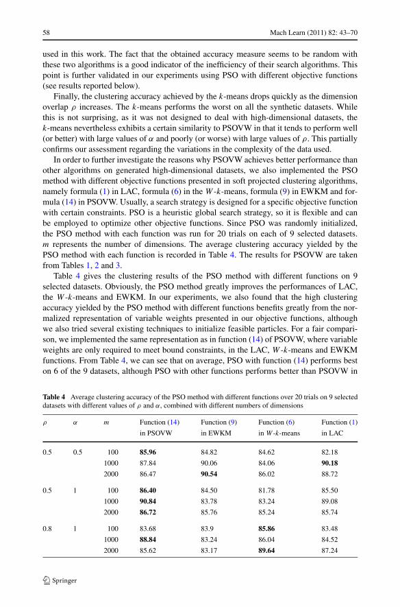
In order to further investigate the reasons why PSOVW achieves better performance thanother algorithms on generated high-dimensional datasets, we also implemented the PSOmethod with different objective functions presented in soft projected clustering algorithms,namely formula (1) in LAC, formula (6) in the W -k-means, formula (9) in EWKM and for-mula (14) in PSOVW. Usually, a search strategy is designed for a specific objective functionwith certain constraints. PSO is a heuristic global search strategy, so it is flexible and canbe employed to optimize other objective functions. Since PSO was randomly initialized,the PSO method with each function was run for 20 trials on each of 9 selected datasets.m represents the number of dimensions. The average clustering accuracy yielded by thePSO method with each function is recorded in Table 4. The results for PSOVW are takenfrom Tables 1, 2 and 3.
Table 4 gives the clustering results of the PSO method with different functions on 9selected datasets. Obviously, the PSO method greatly improves the performances of LAC,the W -k-means and EWKM. In our experiments, we also found that the high clusteringaccuracy yielded by the PSO method with different functions benefits greatly from the nor-malized representation of variable weights presented in our objective functions, althoughwe also tried several existing techniques to initialize feasible particles. For a fair compari-son, we implemented the same representation as in function (14) of PSOVW, where variableweights are only required to meet bound constraints, in the LAC, W -k-means and EWKMfunctions. From Table 4, we can see that on average, PSO with function (14) performs beston 6 of the 9 datasets, although PSO with other functions performs better than PSOVW in
Table 4 Average clustering accuracy of the PSO method with different functions over 20 trials on 9 selecteddatasets with different values of ρ and α, combined with different numbers of dimensions
ρ α m Function (14) Function (9) Function (6) Function (1)
in PSOVW in EWKM in W -k-means in LAC
0.5 0.5 100 85.96 84.82 84.62 82.18
1000 87.84 90.06 84.06 90.18
2000 86.47 90.54 86.02 88.72
0.5 1 100 86.40 84.50 81.78 85.50
1000 90.84 83.78 83.24 89.08
2000 86.72 85.76 85.24 85.74
0.8 1 100 83.68 83.9 85.86 83.48
1000 88.84 83.24 86.04 84.52
2000 85.62 83.17 89.64 87.24
Mach Learn (2011) 82: 43–70 59
some cases. The fact that function (6) is less efficient than functions (1), (9) and (14) is un-derstandable because it uses one weight per dimension; nevertheless, it performs better thanothers on the datasets with large dimension overlap ratios.
The results reported in Tables 1, 2, 3 and 4 suggest that the good performance of PSOVWis due to the PSO method as well as to the normalized representation and the bound con-straints on variable weights in our improved objective function.
In order to see how sensitive the clustering results of these five algorithms are to theinitial cluster centroids, we also examined the variance of 20 clustering results yielded byeach algorithm on each dataset. From Fig. 1, it can be readily seen that PSOVW yields theleast variance in clustering accuracy on most of the datasets. The k-means achieves lowervariance in clustering accuracy than PSOVW on some datasets with 10 clusters, because theclustering accuracy yielded by the k-means on these datasets is always very low. The otherthree soft projected clustering algorithms occasionally work well, achieving low variancein clustering accuracy on some datasets, but their variance is often high. What’s more, itis difficult to tell for which kind of datasets they are less sensitive to the initial centroids.From the three graphs in Fig. 1, we conclude that PSOVW is far less sensitive to the initialcentroids than the other four algorithms.
From Table 5, it is clear that the k-means runs faster than the other four soft projectedclustering algorithms. Although LAC, EWKM and the W -k-means all extend the k-meansclustering process by adding an additional step in each iteration to compute variable weightsfor each cluster, LAC and EWKM are much faster algorithms than the W -k-means ondatasets. The W -k-means required more time to identify clusters, because its objective func-tion involves a much more complicated computation due to the high exponent. Based on thecomputational complexities of the various algorithms and the maximum number of functionevaluations set in each algorithm, PSOVW was supposed to need 5 ∼ 50 times the runningtime the W -k-means requires. In fact, it required only slightly around 4, 2 and 2 times therunning time that the W -k-means spent on the datasets with 100, 1000 and 2000 dimensions,respectively. This is because the update of weights is simpler in PSOVW than in the otherthree soft projected clustering algorithms and particles are evaluated only if they are in thefeasible bound space. We thus conclude that the much more complicated search strategy ofPSOVW allows it to achieve the best clustering accuracy, at an acceptable cost in terms ofrunning time.
Since PSOVW uses more resources than LAC, EWKM and the W -k-means, to ensure avery fair comparison of PSOVW with these three soft projected clustering algorithms, we in-dependently ran LAC, EWKM and the W -k-means multiple times on each dataset and com-pared the best result out of the iterative trials with that of PSOVW. Here, we did not comparePSOVW with k-means, because k-means always works badly on these datasets. Accordingto the average running time of each algorithm reported in Table 5, we ran PSOVW once oneach of the nine datasets. On the datasets with 100, 1000 and 2000 dimensions, LAC andEWKM were run 6, 3 and 3 times respectively and W -k-means was run 4, 2 and 2 timesrespectively. The experimental results in Table 6 still show that PSOVW surpasses the otherthree algorithms on each dataset except on two datasets. This is because particles in PSOVWdo not work independently but cooperate with each other in order to move to better regions.The quality of the clustering is of prime importance and therefore the time taken to obtainit is at most secondary in many clustering applications. To sum up, the much more com-plicated search strategy allows PSOVW to achieve the best clustering accuracy, at a cost oflonger running time, but the running time is acceptable.
60 Mach Learn (2011) 82: 43–70
Fig. 1 Average clustering accuracy and corresponding variance of PSOVW, k-means, W -k-means, EWKMand LAC on each dataset. The horizontal axis represents the 12 datasets in numerical order from 1 to 12 foreach group. The vertical axis represents the variance of 20 clustering accuracies yielded by each algorithmon each dataset
Table 5 Average running time of PSOVW vs. k-means, LAC, W -k-means, and EWKM on the datasets, withvarying m. All times are in seconds
Datasets Running Time (s)
m k-means EWKM LAC W -k-means PSOVW
100 0.42 6.64 7.28 11.95 38.86
1000 3.83 66.17 72.357 119.09 186.572
2000 6.67 131.9 144.51 238.21 310.85
5 Test on real data
5.1 Real-life datasets
A comprehensive performance study was conducted to evaluate our method on real datasets.For the experiments described in this section, we chose three real datasets: the glass identifi-cation dataset (Evett and Spiehler 1987), the Wisconsin breast cancer dataset (Mangasarian
Mach Learn (2011) 82: 43–70 61
Table 6 The comparison of the result of PSOVW once vs. the best result of LAC, EWKM and the W -k-means multiple independent trials on 9 selected datasets with different values of ρ and α, combined withdifferent number of dimensions
ρ α m Algorithms
EWKM LAC W -k-means PSOVW
0.5 0.5 100 75.8 71.2 71.8 89
1000 88.2 71 85.8 84
2000 74.2 67.6 75 85.6
0.5 1 100 82.8 78.2 86.6 89.2
1000 68.8 71.2 74.4 86.4
2000 71 75.4 72.6 88.6
0.8 1 100 82.4 83 86.8 85.4
1000 69.8 77.4 72.4 85
2000 74.2 73 86.0 86.2
and Wolberg 1990) and the insurance company dataset (van der Putten and Someren 2000),which were obtained from the UCI database.3 The glass identification dataset consists of214 instances. Each record has nine numerical variables. The records are classified into twoclasses: 163 window glass instances and 51 non-window glass instances. Wisconsin breastcancer data has 569 instances with 30 continuous variables. Each record is labeled as be-nign or malignant. The dataset contains 357 benign records and 212 malignant records. Theinsurance company dataset has 4000 instances. Each record has 85 numerical variables con-taining information on customers of an insurance company. A classification label indicatingwhether the customer is or is not an insurance policy purchaser is provided with each record.The numbers of purchasers and non-purchasers are 3762 and 238, respectively.
5.2 Results for real data
To study the effect of the initial cluster centroids, we ran each algorithm ten times on eachdataset. Figure 2 presents the average clustering accuracy and the corresponding varianceof each algorithm on each real dataset. The horizontal axis represents real datasets. In theleft graph, the vertical axis represents the average value of the clustering accuracy for eachdataset, and in the right graph it represents the variance of the clustering quality.
From Fig. 2, we can see that PSOVW outperforms the other algorithms. The averageclustering accuracy achieved by PSOVW is high on each dataset, while the correspondingvariance is very low. PSOVW is a random swarm intelligent algorithm; however, its out-puts are very stable. In our experiments, we also observed that other algorithms can achievegood clustering accuracy on the first two datasets on some runs. However, the performancesof LAC and EWKM are very unstable on the glass and breast cancer datasets and the per-formances of the k-means and W -k-means are unstable on the glass dataset. Their aver-age clustering accuracy is not good, because their iterative procedures are derived from thek-means and are very sensitive to the initial cluster centroids. To sum up, PSOVW showsmore capability to cluster these datasets and is more stable than other algorithms.
Fig. 2 Average clustering accuracy and the log variance of the clustering accuracy for each algorithm oneach real-life dataset
6 PSOVW application in text clustering
6.1 Modifications of PSOVW
To further demonstrate the efficiency of PSOVW on real data, we apply it to the problem oftext clustering, called Text Clustering via Particle Swarm Optimization (TCPSO). To extendPSOVW to text clustering, a few modifications to the algorithm are necessary. In particular,we have adopted the conventional tf-idf to represent a text document, and make use of theextended Jaccard coefficient, rather than the Euclidean distance, to measure the similaritybetween two text documents. Throughout this section, we will use the symbols n, m and k
to denote the number of text documents, the number of terms and the number of clusters,respectively. We will use the symbol L to denote the text set, L1,L2, . . . ,Lk to denote eachone of the k categories, and n1, n2, . . . , nk to denote the sizes of the corresponding clusters.
In TCPSO, each document is considered as a vector in the term-space. We used thetf-idf term weighting model (Salton and Buckley 1988), in which each document can berepresented as
[tf1 · log(n/df1), tf2 · log(n/df2), . . . , tfm · log(n/dfm)],where tfi is the frequency of the ith term in the document and dfi is the number of doc-uments that contain the ith term. The extended Jaccard coefficient (Pang-ning et al. 2006)used to measure the similarity between two documents is defined by the following equation:
similarity(x, z) = x · z‖x‖2 + ‖z‖2 − x · z ,
where x represents one document vector, z represents its cluster centroid vector and thesymbol ‘·’ represents the inner product of two vectors. This measure becomes one if twodocuments are identical, and zero if there is nothing in common between them (i.e., thevectors are orthogonal to each other).
Based on the extended Jaccard coefficient, the weighted similarity between two text doc-uments can be represented as follows:
where w is the weight vector for the corresponding cluster whose centroid is z.
Mach Learn (2011) 82: 43–70 63
Therefore, the objective function in TCPSO serves to maximize the overall similarity ofdocuments in a cluster and can be modified as follows:
maxF(W) =k∑
l=1
n∑
i=1
(ul,i · (wβ · x) · (wβ · z)
‖wβ · x‖2 + ‖wβ · z‖2 − (wβ · x) · (wβ · z))
,
where u is the cluster membership of the text document x.
6.2 Text datasets
To demonstrate the effectiveness of TCPSO in text clustering, we first extract four differentstructured datasets from 20 newsgroups.4 The vocabulary, the documents and their corre-sponding key terms as well as the dataset are available in http://people.csail.mit.edu/jrennie/20Newsgroups/. We used the processed version of the 20 news-by-date dataset, which iseasy to read into Matlab, as a matrix. We also selected four large text datasets from theCLUTO clustering toolkit.5 For all datasets, the common words were eliminated using stop-list and all the words were stemmed using Porter’s suffix-stripping algorithm (Porter 1980).Moreover, any terms that occur in fewer than two documents were removed.
We chose three famous clustering algorithms (Bisection k-means, Agglomeration andGraph) and one soft projected clustering algorithm (EWKM) for comparison with TCPSO.For soft projected clustering algorithms, the similarity between two documents is measuredby the extended Jaccard coefficient, while the cosine function is used for the other algo-rithms, namely Bisection k-means, Agglomeration, Graph-based and k-means. The secondgroup of text datasets as well as the three clustering algorithms, Bisection k-means, Ag-glomeration and Graph, can be downloaded from the website of CLUTO.
Table 7 presents four different structured text datasets extracted from 20 newsgroups.Each dataset consists of 2 or 4 categories. ni is the number of documents randomly selectedfrom each category. m and k represent the number of terms and the number of categories,respectively. The categories in datasets 2 and 4 are very closely related to each other, i.e.,the relevant dimensions of different categories overlap considerably, while the categories indatasets 1 and 3 are highly unrelated, i.e., different categories do not share many relevantdimensions. Dataset 2 contains different numbers of documents in each category.
Table 8 summarizes the characteristics of four large text datasets from CLUTO. To en-sure diversity in the datasets, we selected them from different sources. n, m and k arethe number of documents, the number of terms and the number of categories, respec-tively.
Text datasets tr41 & tr45 are derived from TREC collections (TREC 1999). The cate-gories correspond to the documents relevant to particular queries. Text datasets wap & k1bare from the webACE project (Boley et al. 1999; Han et al. 1998), where each documentcorresponds to a web page listed in the subject hierarchy of Yahoo.
6.3 Experimental metrics
The quality of a clustering solution is determined by three different metrics that examinethe class labels of the documents assigned to each cluster. In the following definitions, we
Table 7 The four text datasetsextracted from 20 newsgroups Dataset Source Category ni m k
1 comp.graphics 100 341 2
alt.atheism 100
2 talk.politics.mideast 100 690 2
talk.politics.misc 80
3 comp.graphics 100 434 4
rec.sport.hockey 100
sci.crypt 100
talk.religion.misc 100
4 alt.atheism 100 387 4
rec.sport.baseball 100
talk.politics.guns 100
talk.politics.misc 100
Table 8 The four large textdatasets selected from CLUTO Datasets Source n m k
5: tr41 TREC 878 7454 10
6: tr45 TREC 927 10128 7
7: wap webACE 1560 8460 20
8: k1b webACE 2340 13879 6
Table 9 Experimental metrics
FScore∑k
r=1nrn · max1≤i≤k
2·R(Lr ,Si )·P(Lr ,Si )R(Lr ,Si )+P(Lr ,Si )
, R(Lr ,Si ) = nrinr
,P (Lr , Si ) = nri/mi
Entropy∑k
i=1min · (− 1
log k· ∑k
r=1nrini
· log nrimi
)
assume that a dataset with k categories is grouped into k clusters and n is the total number ofdocuments in the dataset. Given a particular category Lr of size nr and a particular cluster Si
of size mi,nri denotes the number of documents belonging to category Lr that are assignedto cluster Si . Table 9 presents the two evaluation metrics used in this paper.
The first metric is the FScore (Zhao and Karypis 2001), which measures the degree towhich each cluster contains documents from the original category. In the FScore function,R is the recall value and P is the precision value defined for category Lr and cluster Si . Thesecond metric is the Entropy (Zhou et al. 2006), which examines how the documents in allcategories are distributed within each cluster. In general, FScore ranks the clustering qualityfrom zero (worst) to one (best), while Entropy measures from one (worst) to zero (best).The FScore value will be one when every category has a corresponding cluster containingthe same set of documents. The Entropy value will be zero when every cluster contains onlydocuments from a single category.
Mach Learn (2011) 82: 43–70 65
6.4 Experimental results
Evaluations on text datasets 1–4
Our first set of experiments focused on evaluating the average quality of the clustering so-lutions produced by the various algorithms and the influence of text dataset characteristics,such as the number of clusters and the relatedness of clusters, on algorithms. On each small-scale structured text dataset built from 20 newsgroups, we ran the above algorithms 10 times.The average FScore and Entropy values are shown in the following bar graphs. The resultsof the average FScore values for the six algorithms on datasets 1–4 are shown in the leftgraph of Fig. 3, while a similar comparison based on the Entropy measure is presented inthe right graph.
A number of observations can be made by analyzing the results in Fig. 3. First, TCPSO,Bisection k-means and Graph-based yield clustering solutions that are consistently betterthan those obtained by the other algorithms in all experiments on text datasets 1–4. This istrue whether the clustering quality is evaluated using the FScore or the Entropy measure.These three algorithms produced solutions that are about 5–40% better in terms of FScoreand around 5–60% better in terms of Entropy.
Second, TCPSO yielded the best solutions irrespective of the number of clusters, the re-latedness of clusters and the measure used to evaluate the clustering quality. Over the first setof experiments, the solutions achieved by TCPSO are always the best. On average, TCPSOoutperforms the next best algorithm, Graph-based, by around 3–9% in terms of FScore and9–21% in terms of Entropy. In general, it achieves higher FScore values and lower Entropyvalues than the other algorithms. The results in the FScore graph are in agreement with thosein the Entropy graph. Both of them show that it greatly surpasses other algorithms for textclustering.
In general, the performances of TCPSO, Graph-based and Bisection k-means deteriorateon text datasets where categories are highly related. In such documents, each category has asubset of words and two categories share many of the same words. Basically, the probabilityof finding the true centroid for a document varies from one dataset to another, but it decreasesas category relatedness increases. Thus, we would expect that a document can often fail toyield the right centroid regardless of the metric used.
Third, except for the Entropy measure on text datasets 1 and 4, Graph-based performs thenext best for both FScore and Entropy. Bisection k-means also performs quite well when the
Fig. 3 FScore and Entropy values of each algorithm on datasets 1–4
66 Mach Learn (2011) 82: 43–70
categories in datasets are highly unrelated. EWKM always performs in the middle range, dueto its employment of the local search strategy. The solutions yielded by the k-means fluctuatein all experiments. Agglomeration performs the worst of the six algorithms, yielding smallFScore and large Entropy values on all datasets. This means the number of documents fromeach cluster yielded by Agglomeration is thus more balanced in one genuine category andas a result, the number of documents that are correctly identified by Agglomeration in thegenuine category is very low.
Evaluations on text datasets 5–8
To further investigate the behavior of TCPSO, we performed a second series of experi-ments, focused on evaluating the comprehensive performance of each algorithm on largetext datasets. Each algorithm was independently run 10 times on each of datasets 5–8. Theaverage FScore values for the six algorithms on datasets 1–4 are shown in the left graph ofFig. 4, while a similar comparison based on the Entropy measure is presented in the rightgraph.
Looking at the two graphs of Fig. 4 and comparing the performance of each algorithmon datasets 5–8, we can see that TCPSO outperformed all other algorithms, on average,although Graph-based and Bisection k-means are very close. Graph-based and Bisectionk-means are respectively worse than TCPSO in terms of FScore by 1–11% and 6–10%,on average, while they yield similar Entropy values to TCPSO. That means each categoryof documents is mainly distributed within its dominant cluster and TCPSO recovers moredocuments of each cluster primarily from their original categories.
Although Graph-based and Bisection k-means performed quite well on the datasets tr41and k1b, their performances deteriorate sharply on the datasets tr45 & wap, where there isconsiderable overlap between the key words of different categories, such as the categoriescable and television, multimedia and media etc. They failed to perform well on such datasets,while TCPSO still achieved relatively high FScore values because it indentifies clustersembedded in subspaces by iteratively assigning an optimal feature weight vector to eachcluster. The other three algorithms occasionally work well, achieving FScore values above0.8 on the dataset k1b, whose categories (business, politics, sports etc.) are highly unrelated,but the FScore values are relatively low on other datasets. Moreover, their correspondingEntropy values are very high, which means each category of documents is more evenlydistributed within all the clusters.
Fig. 4 Average FScore and Entropy values of each algorithm on datasets 5–8
Mach Learn (2011) 82: 43–70 67
7 Conclusions
In response to the needs arising from the emergence of high-dimensional datasets in datamining applications and the low cluster quality of projected clustering algorithms, this pa-per proposed a particle swarm optimizer for the variable weighting problem, called PSOVW.The selection of the objective function and the search strategy is very important in soft pro-jected clustering algorithms. PSOVW employs a k-means weighting function, which calcu-lates the sum of the within-cluster distance for each cluster along relevant dimensions pref-erentially to irrelevant ones. It also proposes a normalized representation of variable weightsin the objective function, which greatly facilities the search process. Finally, the new algo-rithm makes use of particle swarm optimization to get near-optimal variable weights for thegiven objective function. Although PSOVW runs more slowly than other algorithms, its defi-ciency in running time is acceptable. Experimental results on synthetic and real-life datasets,including an application to document clustering, show that it can greatly improve clusteringaccuracy for high-dimensional data and is much less sensitive to the initial cluster centroids.Moreover, the application to text clustering shows that the effectiveness of PSOVW is notconfined to Euclidean distance. The reason is that the weights are only affected by the valuesof the objective function and weight updating in PSOVW is independent of the similaritymeasure. Other similarity measures can thus be used for different applications: the extendedJaccard coefficient for text data, for instance.
Two issues need to be addressed by the PSOVW algorithm. PSOVW is still not ableto recover the relevant dimensions totally. In fact, none of the tested algorithms, includ-ing PSOVW, consistently identify the relevant dimensions to achieve their final cluster-ing results; i.e., some irrelevant dimensions may have high weights while some relevantdimensions may have low weights. The dimensionality of the datasets and the numberof relevant dimensions for each cluster are extremely high compared to the number ofdata points, resulting in very sparse datasets. This might be the main reason why thesealgorithms fail to recover all the relevant dimensions. Further investigations are needed.The other major issue in PSOVW is that usually the structure of the data is completelyunknown in real-world data mining applications and it is thus very difficult to providethe number of clusters k. Although a number of different approaches for determiningthe number of clusters automatically have been proposed (Tibshirani and Walther 2000;Handl and Knowles 2004), no reliable method exists to date, especially for high-dimensionalclustering. In the Ph.D. work of the first author, Yanping (2009), the PSOVW has beenextended to deal also with the problem of automatically determining the number of clus-ters k.
Acknowledgements We are thankful to Prof. Suganthan for providing the Matlab coding of CLPSO. Wethank Tengke Xiong and Yassine Parakh Ousman for their help with the DiSH and HARP algorithms. Wealso thank the anonymous reviewers for their constructive comments on our manuscript.
Appendix
The algorithm for generating a synthetic dataset is derived from but not identical to the onepresented in Jing et al. (2007).
– Specify the number of clusters k, the number of dimensions m and the number of ob-jects n. Set three parameters, ε,ρ and α.
68 Mach Learn (2011) 82: 43–70
– // Determine relevant dimensions for each cluster.// Determine the number of relevant dimensions ml for each cluster.For each cluster l,
Assign a random number ml ∈ [2,m], where∑
ml = ε ∗ k ∗ m.
For each cluster l,If l == 1,
Randomly choose m1 relevant dimensions for C1.Otherwise,
Randomly choose ρ ∗ml relevant dimensions from the relevant dimensions of Cl−1.Randomly choose (1 − ρ) ∗ ml relevant dimensions from the other dimensions.
End.
– //Generate the mean u and the variance σ for each relevant dimension of each cluster.σ = 1;For each cluster l,
If the relevant dimension j is not a common relevant dimension of clusters Cl andCl−1,
Randomly set ul,j in [0,100].Otherwise,
If (ul−1,j + α ∗ σ) > 100,ul,j = ul−1,j − α ∗ σ .
Otherwise,ul,j = ul−1,j + α ∗ σ .
End.End.
– //Generate data points for each cluster.For each cluster l,
//Specify the number of points nl .nl = n/k;For each dimension j ,
If j is a relevant dimension of Cl,
Produce the data points with a normal distribution, N(ul,j , σ ).Otherwise,
Uniformly produce the data points in [0,10].End.
References
Agrawal, R., Gehrke, J., Gunopulos, D., & Raghavan, P. (2005). Automatic subspace clustering of high di-mensional data. Data Mining and Knowledge Discovery, 11(1), 5–33.
Aitnouri, E., Wang, S., & Ziou, D. (2000). On comparison of clustering techniques for histogram pdf estima-tion. Pattern Recognition and Image Analysis, 10(2), 206–217.
Boley, D., Gini, M., et al. (1999). Document categorization and query generation on the world wild web usingWebACE. AI Review, 11, 365–391.
Bouguessa, M., Wang, S., & Sun, H. (2006). An objective approach to cluster validation. Pattern RecognitionLetters, 27(13), 1419–1430.
Domeniconi, C., Gunopulos, D., Ma, S., Yan, B., Al-Razgan, M., & Papadopoulos, D. (2007). Locally adap-tive metrics for clustering high dimensional data. Data Mining and Knowledge Discovery Journal, 14,63–97.
Mach Learn (2011) 82: 43–70 69
Eberhart, R. C., & Kennedy, J. (1995). A new optimizer using particle swarm theory. In Proc. 6th interna-tional symposium on micromachine and human science, Japan (pp. 39–43).
Elke, A., Christian, B., et al. (2008). Detection and visualization of subspace cluster hierarchies. In LNCS(Vol. 4443, pp. 152–163). Berlin: Springer.
Evett, I. W., & Spiehler, E. J. (1987). Rule induction in forensic science. Central Research Establishment.Home Office Forensic Science Service, Aldermaston, Reading, Berkshire RG7 4PN.
Goil, G. S., Nagesh, H., & Choudhary, A. (1999). Mafia: Efficient and scalable subspace clustering for verylarge data sets. Technical Report CPDC-TR-9906-010, Northwestern University.
Han, E. H., Boley, D., et al. (1998). WebACE: A web agent for document categorization and exploration. InProc. of 2nd international conf. on autonomous agents.
Handl, J., & Knowles, J. (2004). Multiobjective clustering with automatic determination of the number ofclusters. Technical Report, UMIST, Department of Chemistry.
Huang, J. Z., Ng, M. K., Rong, H., & Li, Z. (2005). Automated dimension weighting in k-means type clus-tering. IEEE Transactions on Pattern Analysis and Machine Intelligence, 27(5), 1–12.
Jing, L., Ng, M. K., & Huang, J. Z. (2007). An entropy weighting k-means algorithm for subspace clusteringof high-dimensional sparse data. IEEE Transactions on Knowledge and Data Engineering, 19(8), 1026–1041.
Kriegel, H.-P., Kroger, P., & Zimek, A. (2009). Clustering high-dimensional data: A survey on subspace clus-tering, pattern-based clustering, and correlation clustering. ACM Transactions on Knowledge DiscoveryData, 3(1), Article 1.
Liang, J. J., Qin, A. K., Suganthan, P. N., & Baskar, S. (2006). Comprehensive learning particle swarmoptimizer for global optimization of multimodal functions. IEEE Transactions on Evolutionary Compu-tation, 10(3), 281–295.
Lu, Y. (2009). Particle swarm optimizer: applications in high-dimensional data clustering. Ph.D. Disserta-tion, University of Sherbrooke, Department of Computer Science.
Makarenkov, V., & Legendre, P. (2001). Optimal variable weighting for ultrametric and additive trees andk-means partitioning: Methods and software. Journal of Classification, 18(2), 245–271.
Mangasarian, O. L., & Wolberg, W. H. (1990). Breast cancer diagnosis via linear programming. SIAM News,23(5), 1–18.
Moise, G., & Sander, J. (2008). Finding non-redundant, statistically significant regions in high dimensionaldata: A novel approach to projected and subspace clustering. In Proc. of the 14th ACM SIGKDD inter-national conference on knowledge discovery and data mining (pp. 533–541).
Moise, G., Sander, J., & Ester, M. (2008). Robust projected clustering. Knowledge and Information Systems,14(3), 273–298.
Onwubolu, G. C., & Clerc, M. (2004). Optimal operating path for automated drilling operations by a newheuristic approach using particle swarm optimization. International Journal of Production Research,42(3), 473–491.
Pang-ning, T., Michael, S., & Vipin, K. (2006). Introduction to data mining (p. 77). Upper Saddle River:Pearson Education.
Parsons, L., Haque, E., & Liu, H. (2004). Subspace clustering for high dimensional data: A review. SIGKDDExplorations Newsletter, 6, 90–105.
Porter, M. F. (1980). An algorithm for suffix stripping. Program, 14(3), 130–137.Procopiuc, C. M., Jones, M., Agarwal, P. K., & Murali, T. M. (2002). A Monte Carlo algorithm for fast pro-
jective clustering. In Proc. of ACM SIGMOD international conference on management of data (pp. 418–427).
Salman, A., Ahmad, I., & Al-Madani, S. (2003). Particle swarm optimization for task assignment problem.Microprocessors and Microsystems, 26(8), 363–371.
Salton, G., & Buckley, C. (1988). Term-weighting approaches in automatic text retrieval. InformationProcessing & Management, 24(5), 513–523.
Tasgetiren, M. F., Sevkli, M., Liang, Y.-C., & Gencyilmaz, G. (2004). Particle swarm optimization algorithmfor single machine total weighted tardiness problem. In Proc. of the 2004 congress on evolutionarycomputation (CEC’04), Portland, Oregon (pp. 1412–1419).
TREC (1999). Text retrieval conference, http://trec.nist.gov/.Tibshirani, R., Walther, G., et al. (2000). Estimating the number of clusters in a dataset via the Gap Statistic.
Technical Report, Stanford Univeristy.Van den Bergh, F., & Engelbecht, A. P. (2000). Cooperative learning in neural networks using particle swarm
optimizers. South African Computer Journal, 26, 84–90.van der Putten, P., & van Someren, M. (Eds.) (2000). CoIL challenge 2000: the insurance company case.
Published by Sentient Machine Research, Amsterdam. Technical Report.Woo, K.-G., Lee, J.-H., Kim, M.-H., & Lee, Y.-J. (2004). FINDIT: A fast and intelligent subspace clustering
algorithm using dimension voting. Information and Software Technology, 46(4), 255–271.
Yoshida, H., Kawata, K., Fukuyama, Y., & Nakanishi, Y. (2000). A particle swarm optimization for reac-tive power and voltage control considering voltage security assessment. IEEE Transactions on PowerSystems, 15(4), 1232–1239.
Zhao, Y., & Karypis, G. (2001). Criterion functions for document clustering: Experiments and analysis.Technical Report, CS Dept., Univ. of Minnesota.
Zhou, X., Hu, X., Zhang, X., Lin, X., & Song, I.-Y. (2006). Context-sensitive semantic smoothing for thelanguage modeling approach to genomic IR. In SIGIR’06.