24
Particle Systems 1 Adapted from: E. Angel and D. Shreiner: Interactive Computer Graphics 6E © Addison-Wesley 2012
| Date post: | 19-Dec-2015 |
| Category: |
Documents |
| Upload: | loreen-mills |
| View: | 215 times |
| Download: | 0 times |
Particle Systems
1Adapted from: E. Angel and D. Shreiner: Interactive Computer Graphics 6E © Addison-Wesley 2012

2
Particle Systems
• loosely defined modeling, or rendering, or animation
• key criteria collection of particles random element controls attributes
• position, velocity (speed and direction), color, lifetime, age, shape, size, transparency
• predefined stochastic limits: bounds, variance, type of distribution
3E. Angel and D. Shreiner: Interactive Computer Graphics 6E © Addison-Wesley 2012
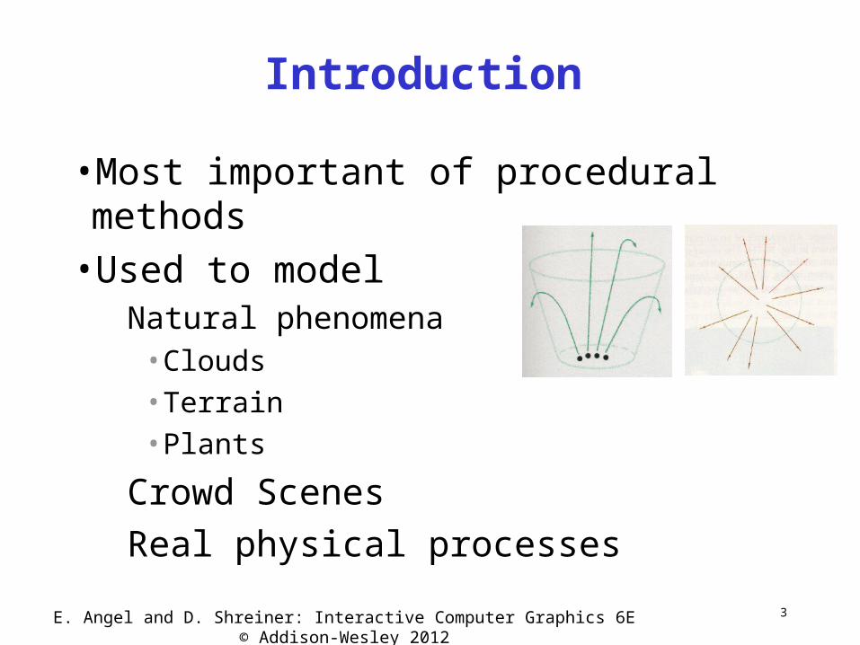
Introduction
•Most important of procedural methods•Used to model
Natural phenomena• Clouds• Terrain• Plants
Crowd Scenes
Real physical processes

4
Particle Systems Demos
•general particle systems http://www.wondertouch.com
•boids: bird-like objects http://www.red3d.com/cwr/boids/
5
Particle Life Cycle
• generation randomly within “fuzzy” location
initial attribute values: random or fixed
• dynamics attributes of each particle may vary over time
• color darker as particle cools off after explosion
can also depend on other attributes• position: previous particle position + velocity + time
• death age and lifetime for each particle (in frames)
or if out of bounds, too dark to see, etc
6
Particle System Rendering
•expensive to render thousands of particles•simplify: avoid hidden surface calculations
each particle has small graphical primitive (blob)
pixel color: sum of all particles mapping to it
• some effects easy temporal anti-aliasing (motion blur)
• normally expensive: supersampling over time• position, velocity known for each particle• just render as streak
7E. Angel and D. Shreiner: Interactive Computer Graphics 6E © Addison-Wesley 2012
Newtonian Particle
•Particle system is a set of particles•Each particle is an ideal point mass•Six degrees of freedom
Position
Velocity
•Each particle obeys Newtons’ law
f = ma

8E. Angel and D. Shreiner: Interactive Computer Graphics 6E © Addison-Wesley 2012
Particle Equations
pi = (xi, yi zi)
vi = dpi /dt = pi‘ = (dxi /dt, dyi /dt , zi /dt)
m vi‘= fi
Hard part is defining force vector

9E. Angel and D. Shreiner: Interactive Computer Graphics 6E © Addison-Wesley 2012
Force Vector
• Independent Particles Gravity
Wind forces
O(n) calulation
•Coupled Particles O(n) Meshes
Spring-Mass Systems
•Coupled Particles O(n2) Attractive and repulsive forces

10E. Angel and D. Shreiner: Interactive Computer Graphics 6E © Addison-Wesley 2012
Solution of Particle Systems
float time, delta state[6n], force[3n];state = initial_state();for(time = t0; time<final_time, time+=delta) {force = force_function(state, time);state = ode(force, state, time, delta);render(state, time)}

11E. Angel and D. Shreiner: Interactive Computer Graphics 6E © Addison-Wesley 2012
Simple Forces
•Consider force on particle i
fi = fi(pi, vi)
•Gravity fi = g
gi = (0, -g, 0)
•Wind forces•Drag
pi(t0), vi(t0)

12E. Angel and D. Shreiner: Interactive Computer Graphics 6E © Addison-Wesley 2012
Meshes
•Connect each particle to its closest neighbors
O(n) force calculation
•Use spring-mass system

13E. Angel and D. Shreiner: Interactive Computer Graphics 6E © Addison-Wesley 2012
Spring Forces
•Assume each particle has unit mass and is connected to its neighbor(s) by a spring
•Hooke’s law: force proportional to distance (d = ||p – q||) between the points

14E. Angel and D. Shreiner: Interactive Computer Graphics 6E © Addison-Wesley 2012
Hooke’s Law
•Let s be the distance when there is no force
f = -ks(|d| - s) d/|d|
ks is the spring constant
d/|d| is a unit vector pointed from p to q•Each interior point in mesh has four forces applied to it

15E. Angel and D. Shreiner: Interactive Computer Graphics 6E © Addison-Wesley 2012
Spring Damping
•A pure spring-mass will oscillate forever•Must add a damping term
f = -(ks(|d| - s) + kd d·d/|d|)d/|d|
•Must project velocity
·

16E. Angel and D. Shreiner: Interactive Computer Graphics 6E © Addison-Wesley 2012
Attraction and Repulsion
• Inverse square law
f = -krd/|d|3
•General case requires O(n2) calculation• In most problems, the drop off is such that not many particles contribute to the forces on any given particle
•Sorting problem: is it O(n log n)?
17E. Angel and D. Shreiner: Interactive Computer Graphics 6E © Addison-Wesley 2012
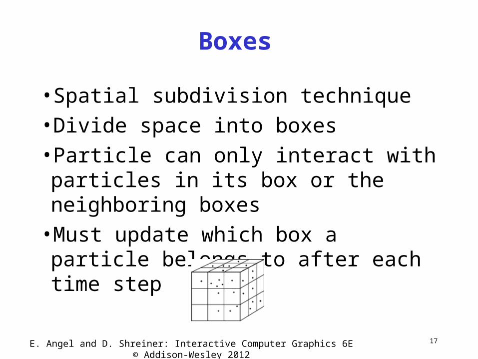
Boxes
•Spatial subdivision technique•Divide space into boxes•Particle can only interact with particles in its box or the neighboring boxes
•Must update which box a particle belongs to after each time step
18E. Angel and D. Shreiner: Interactive Computer Graphics 6E © Addison-Wesley 2012
Particle Field Calculations
•Consider simple gravity•We don’t compute forces due to sun, moon, and other large bodies
•Rather we use the gravitational field•Usually we can group particles into equivalent point masses

19E. Angel and D. Shreiner: Interactive Computer Graphics 6E © Addison-Wesley 2012
Solution of ODEs
•Particle system has 6n ordinary differential equations
•Write set as du/dt = g(u,t)
•Solve by approximations using Taylor’s Thm

20E. Angel and D. Shreiner: Interactive Computer Graphics 6E © Addison-Wesley 2012
Euler’s Method
u(t + h) ≈ u(t) + h du/dt = u(t) + hg(u, t)
Per step error is O(h2)
Require one force evaluation per time step
Problem is numerical instability
depends on step size
21E. Angel and D. Shreiner: Interactive Computer Graphics 6E © Addison-Wesley 2012
Improved Euler
u(t + h) ≈ u(t) + h/2(g(u, t) + g(u, t+h))
Per step error is O(h3)
Also allows for larger step sizes
But requires two function evaluations per step
Also known as Runge-Kutta method of order 2
22E. Angel and D. Shreiner: Interactive Computer Graphics 6E © Addison-Wesley 2012
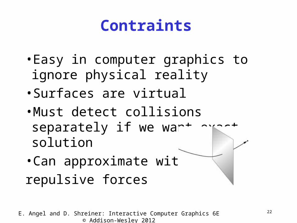
Contraints
•Easy in computer graphics to ignore physical reality
•Surfaces are virtual•Must detect collisions separately if we want exact solution
•Can approximate with
repulsive forces

23E. Angel and D. Shreiner: Interactive Computer Graphics 6E © Addison-Wesley 2012
Collisions
Once we detect a collision, we can calculate new path
Use coefficient of resititution
Reflect vertical component
May have to use partial time step

24E. Angel and D. Shreiner: Interactive Computer Graphics 6E © Addison-Wesley 2012
Contact Forces


