60
Particles
| Date post: | 17-Sep-2018 |
| Category: |
Documents |
| Upload: | truongminh |
| View: | 216 times |
| Download: | 0 times |

Particles

Simulation Homework
• Build a particle system based either on F=ma or procedural simulation
– Examples: Smoke, Fire, Water, Wind, Leaves, Cloth, Magnets, Flocks, Fish, Insects, Crowds, etc.
• Simulate a rigid body
– Examples: Angry birds, Bodies tumbling, bouncing, moving around in a room and colliding, Explosions & Fracture, Drop the camera, Etc…
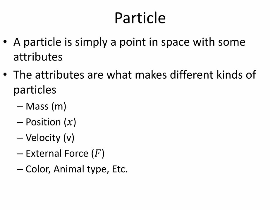
Particle
• A particle is simply a point in space with some attributes
• The attributes are what makes different kinds of particles
– Mass (m)
– Position (𝑥)
– Velocity (v)
– External Force (𝐹)
– Color, Animal type, Etc.
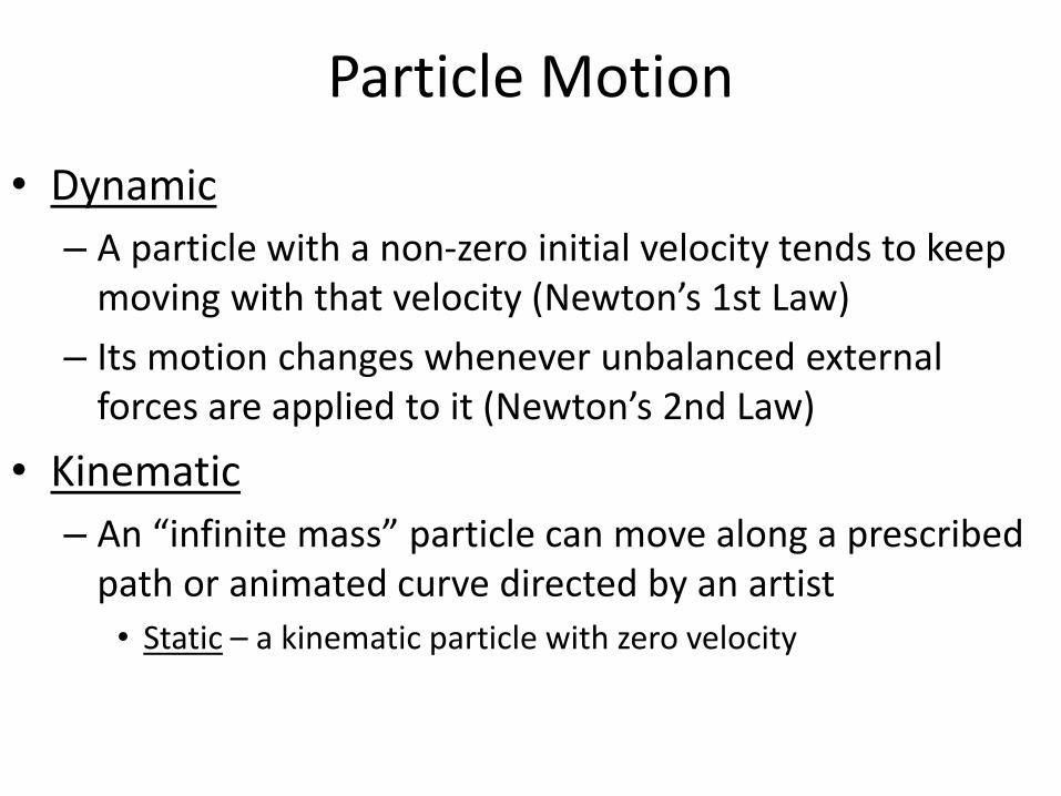
Particle Motion
• Dynamic
– A particle with a non-zero initial velocity tends to keep moving with that velocity (Newton’s 1st Law)
– Its motion changes whenever unbalanced external forces are applied to it (Newton’s 2nd Law)
• Kinematic
– An “infinite mass” particle can move along a prescribed path or animated curve directed by an artist
• Static – a kinematic particle with zero velocity

Dynamics

Newton’s Second Law
• The net force on an object is equal to the rate of change of its linear momentum P=mv
𝐹 =𝑑𝑃
𝑑𝑡=𝑑(𝑚𝑣)
𝑑𝑡= 𝑚𝑎
• The last equality holds if the object has constant mass
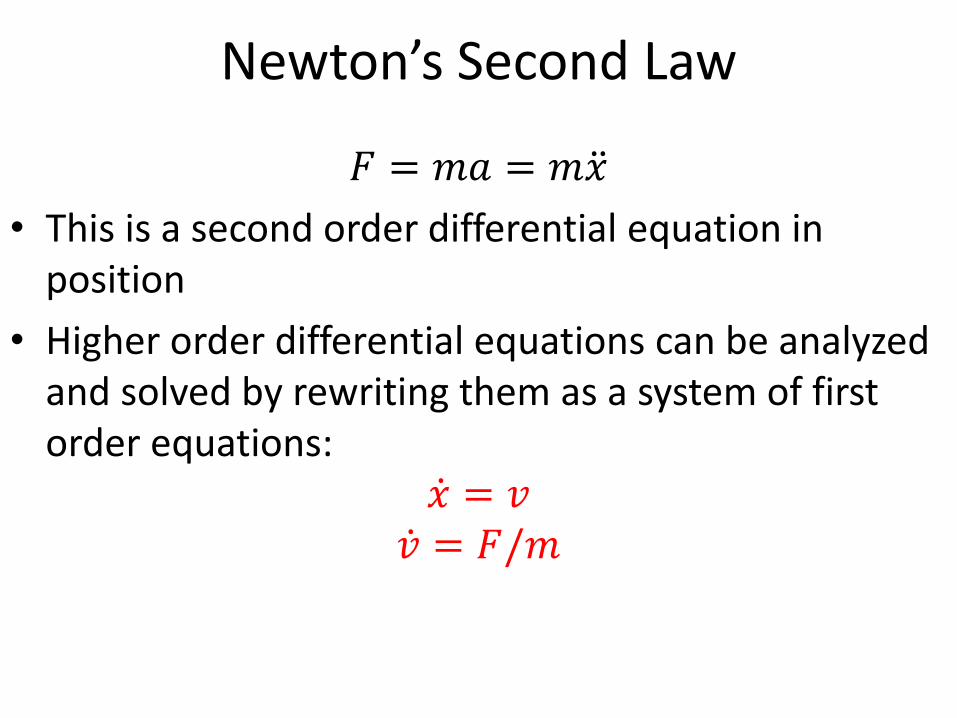
Newton’s Second Law
𝐹 = 𝑚𝑎 = 𝑚 ሷ𝑥
• This is a second order differential equation in position
• Higher order differential equations can be analyzed and solved by rewriting them as a system of first order equations:
ሶ𝑥 = 𝑣ሶ𝑣 = 𝐹/𝑚

Forces
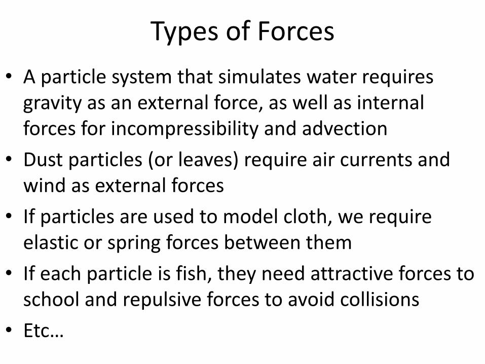
Types of Forces
• A particle system that simulates water requires gravity as an external force, as well as internal forces for incompressibility and advection
• Dust particles (or leaves) require air currents and wind as external forces
• If particles are used to model cloth, we require elastic or spring forces between them
• If each particle is fish, they need attractive forces to school and repulsive forces to avoid collisions
• Etc…
Types of forces
• Constant forces (e.g. gravity)
• Time dependent forces (e.g. wind)
• Position dependent forces (e.g. force fields, spatially varying wind)
• Velocity dependent forces (e.g. drag, friction)
• Position & Velocity dependent forces (e.g. springs)

Gravity• 𝐹𝑔𝑟𝑎𝑣 = −𝑚𝑔
• 𝑔 = 9.8 𝑚/𝑠2 is a constant
• 𝑚 is the mass of the body/particle
• Simple ballistic motion…

Wind
• Position and time dependent force
• 𝑓𝑤𝑖𝑛𝑑 = 𝑓( Ԧ𝑥, 𝑡)
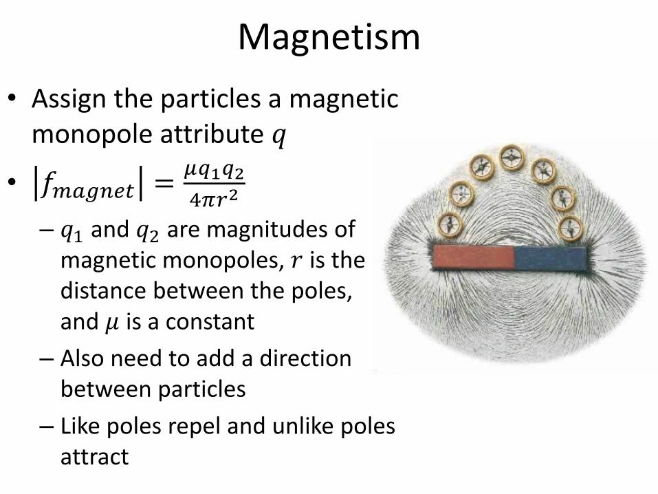
Magnetism
• Assign the particles a magnetic monopole attribute 𝑞
• 𝑓𝑚𝑎𝑔𝑛𝑒𝑡 =𝜇𝑞1𝑞2
4𝜋𝑟2
– 𝑞1 and 𝑞2 are magnitudes of magnetic monopoles, 𝑟 is the distance between the poles, and 𝜇 is a constant
– Also need to add a direction between particles
– Like poles repel and unlike poles attract
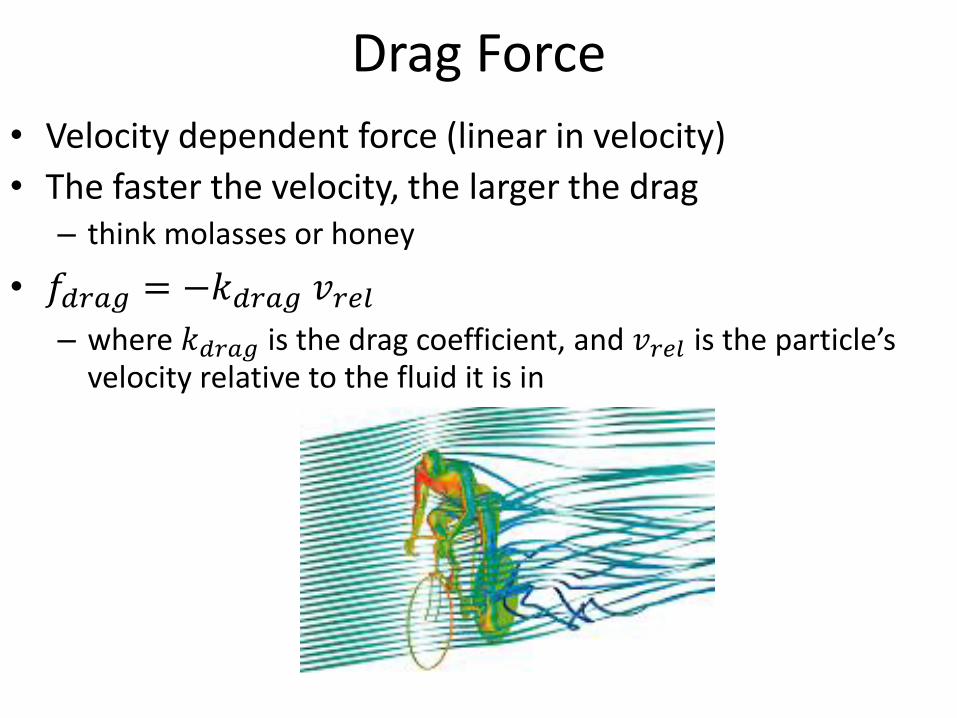
Drag Force
• Velocity dependent force (linear in velocity)
• The faster the velocity, the larger the drag– think molasses or honey
• 𝑓𝑑𝑟𝑎𝑔 = −𝑘𝑑𝑟𝑎𝑔 𝑣𝑟𝑒𝑙– where 𝑘𝑑𝑟𝑎𝑔 is the drag coefficient, and 𝑣𝑟𝑒𝑙 is the particle’s
velocity relative to the fluid it is in
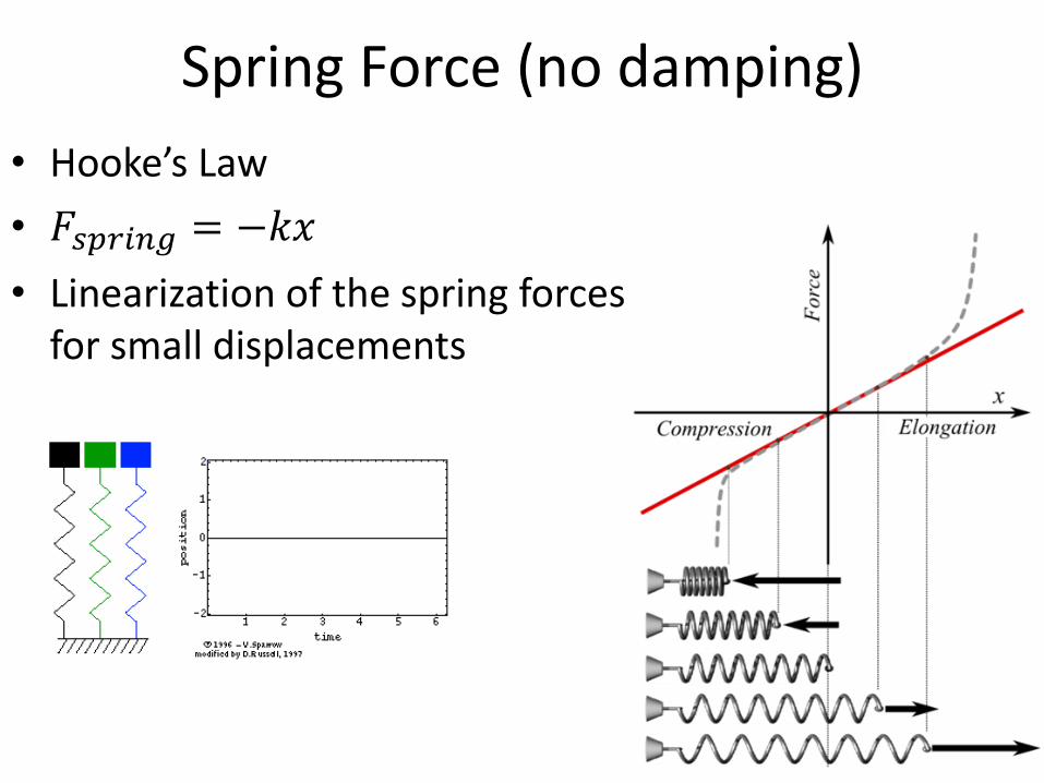
Spring Force (no damping)
• Hooke’s Law
• 𝐹𝑠𝑝𝑟𝑖𝑛𝑔 = −𝑘𝑥
• Linearization of the spring forces for small displacements

Spring Force (with damping)
• 𝐹𝑠𝑝𝑟𝑖𝑛𝑔 = −𝑘𝑥 − 𝑘𝑑 ሶ𝑥
• Adds an exponential decay to the amplitude of oscillation
• It is a good practice to add some damping to physical systems to keep them form going unstable
– and for realism

Question #1
LONG FORM:• Briefly discuss various types of forces that can be
used in video game simulations • Answer short form question below
SHORT FORM:• Can you think of a use for forces in your video
game? Briefly explain• (Notice I’m starting to assume you have a video
game idea. Do you? ☺)

Collision Detection
Collisions
• As particles move around under the influence of gravity, drag, and other forces, how do they interact with other objects?
• This is where collisions come into play
• How do we detect collisions?
– Check to see if a particle is inside some object
Example: Plane
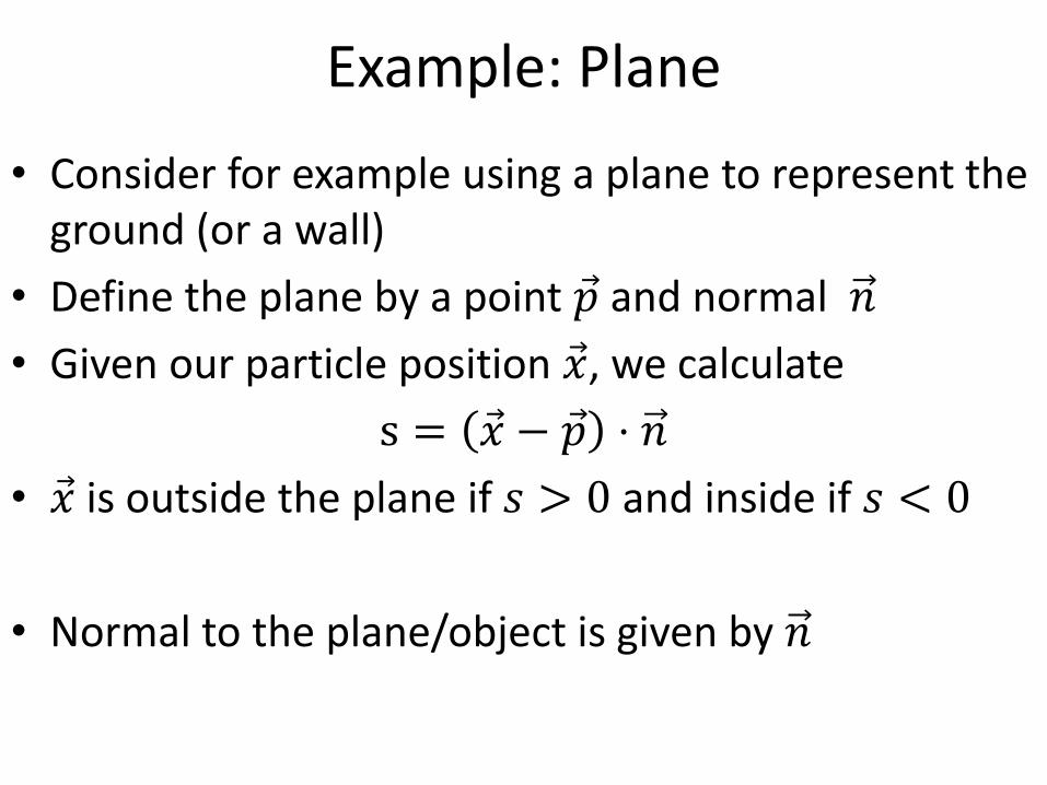
• Consider for example using a plane to represent the ground (or a wall)
• Define the plane by a point Ԧ𝑝 and normal 𝑛
• Given our particle position Ԧ𝑥, we calculate
s = Ԧ𝑥 − Ԧ𝑝 ⋅ 𝑛
• Ԧ𝑥 is outside the plane if 𝑠 > 0 and inside if 𝑠 < 0
• Normal to the plane/object is given by 𝑛

Example: Box
• Use a plane for each of the six faces of the box
• If the particle is inside all 6 faces, it is inside the box
• To find the normal, one has to identify the closest of the 6 planes
• This is given by the value of 𝑠 closest to zero
• Can be used for other convex polyhedra as well

Example: Sphere
• Define a sphere with a center Ԧ𝑐 and a radius r
• Given a point Ԧ𝑞, calculate 𝑠 = Ԧ𝑞 − Ԧ𝑐 − 𝑟.
• Ԧ𝑞 is outside the sphere if 𝑠 > 0 and inside if 𝑠 < 0
• Normal at the point is ( Ԧ𝑞 − Ԧ𝑐)/ Ԧ𝑞 − Ԧ𝑐

Collision Response
Collision Response
• Do something to take the bodies from a “colliding state” to a “non-colliding state”
• What properties should a good response algorithm have?
– Remove interpenetrations
– Conserve linear and angular momentum
– Have the correct relative velocities based on the material properties of the colliding bodies
– Should look plausible!
Collision Response (Notation Key)
• 𝑐𝑅 is the coefficient of restitution• 0 is completely inelastic; objects stick together
• 1 is completely elastic; objects bounce without losing any kinetic energy
• Between 0 and 1 means some energy is lost due to deformation, damage, sound, heat, etc.
• 𝑚𝑎 is the mass of the first object
• 𝑚𝑏 is the mass of the second object
• 𝑢𝑎 is the velocity of the first object before impact
• 𝑢𝑏 is the velocity of the second object before impact
• 𝑣𝑎 is the velocity of the first object after impact
• 𝑣𝑏 is the velocity of the second object after impact

Collision Response (Formulas)
𝑐𝑅 = −𝑣𝑏 − 𝑣𝑎𝑢𝑏 − 𝑢𝑎
(definition)
𝑚𝑎𝑢𝑎 +𝑚𝑏𝑢𝑏 = 𝑚𝑎𝑣𝑎 +𝑚𝑏𝑣𝑏 (momentum conservation)
• Two equations in two unknowns, solve…
• 𝑣𝑎 =𝑚𝑎 𝑢𝑎 +𝑚𝑏 𝑢𝑏 −𝑚𝑏 𝑐𝑅 𝑢𝑎−𝑢𝑏
𝑚𝑎+𝑚𝑏
• 𝑣𝑏 =𝑚𝑎 𝑢𝑎 +𝑚𝑏 𝑢𝑏 −𝑚𝑎 𝑐𝑅 𝑢𝑏−𝑢𝑎
𝑚𝑎+𝑚𝑏
• We can also look at this in terms of an impulse. The impulse required to change the velocity of object a is
𝑗 = 𝑚𝑎(𝑣𝑎 − 𝑢𝑎)
• An equal and opposite impulse is applied to object b

If one object is infinitely heavy…
• Useful for kinematic objects (stationary or moving)
• Make 𝑚𝑏 infinite
• 𝑣𝑏 = 𝑢𝑏 (doesn’t change)
• 𝑣𝑎 =𝑚𝑏 𝑢𝑏 −𝑚𝑏 𝐶𝑅 𝑢𝑎−𝑢𝑏
𝑚𝑏= 𝑢𝑏 − 𝑐𝑅 𝑢𝑎 − 𝑢𝑏
• If 𝑢𝑏 = 0 (stationary object, e.g. ground plane), then this further simplifies to 𝑣𝑎 = −𝑐𝑅𝑢𝑎
Collisions in 3D

Higher Spatial Dimensions
• The prior equations describe collision in 1D only
• In 3D, they describe the collision in the normal direction, i.e. on the components of velocity (dot product-ed) into the normal direction
• The tangential components of the velocity do not change, unless there is collisional friction
• Since most surfaces can be locally approximated as being planar, let’s consider point plane collisions….

Point-Plane Collision Response
𝑉
𝑃
𝑁
𝑉𝑁 = 𝑉 ⋅ 𝑁 𝑁
𝑉𝑇 = 𝑉 − 𝑉𝑁
𝑉𝑁
𝑉𝑇
• Collision only affects the normal component of velocity
• As such, split the velocity into a normal and tangent component:
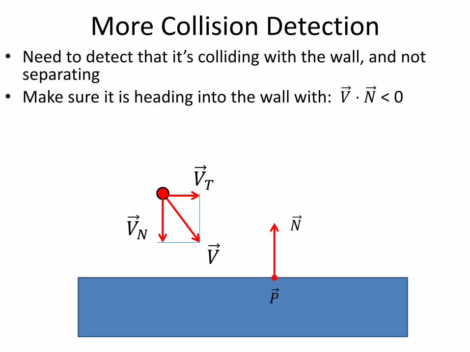
More Collision Detection• Need to detect that it’s colliding with the wall, and not
separating• Make sure it is heading into the wall with: 𝑉 ⋅ 𝑁 < 0
𝑃
𝑁𝑉𝑁
𝑉𝑇
𝑉

Collision Response• Adjust the normal velocity of the particle to account for
the collision
• Leave the tangential velocity unchanged
• Probably also want to adjust the position of the particle to move it to the surface of the object (if it is inside)
𝑉
𝑉𝑁
𝑉𝑇
𝑉′
−𝑐𝑅𝑉𝑁
𝑉𝑇
𝑉′ = 𝑉𝑇 − 𝑐𝑅𝑉𝑁

Friction• Let 𝑗𝑛 be the collision impulse in the normal direction
• The new tangential velocity is 𝑉𝑇′ = 𝑉𝑇 −
𝜇 Ԧ𝑗𝑛 𝑉𝑇
𝑚 𝑉𝑇, where 𝜇 is
the coefficient of kinetic friction:
• The clamping ensures that friction slows a particle down without changing its direction
• Static friction can be modeled by first applying this formula with the (typically larger) static friction coefficient– If the max clamps to 0, static friction stopped the object from
moving
– If not, then recompute the formula with the smaller kinetic friction coefficient
𝑉′ = 𝑚𝑎𝑥 0, 1 −𝜇 Ԧ𝑗𝑛𝑚 𝑉𝑇
𝑉𝑇 − 𝑐𝑅𝑉𝑁

Question #2
LONG FORM:• Briefly discuss implementing collisions• Answer short form question below
SHORT FORM:• Can you think of a good use for collisions in your
video game? Briefly explain

ODEs

Ordinary Differential Equations (ODEs)
• An ODE is an equation containing a function of one independent variable t and its derivatives:
𝑓 𝑡, 𝑦, 𝑦′, 𝑦′′, … = 0
• First order ODE’s have at most one derivative:
𝑓 𝑡, 𝑦, 𝑦′ = 0
• If we can isolate the derivative term, we call it an explicit ODE (otherwise its implicit):
𝑦′ = 𝑓(𝑡, 𝑦)

• Model problem
• linear ODE 𝑦′ = 𝜆𝑦– solution is 𝑦 = 𝑦𝑜𝑒
𝜆(𝑡−𝑡0)
– 3 kinds of solutions
• 𝜆 > 0 ill-posed (a)
• 𝜆 = 0 mildly ill-posed (b)
• 𝜆 < 0 well-posed (c)
• Ill-posed problems can not (should not) be solved (with any reasonable assurances) on the computer
Well-Posed vs. Ill-Posed ODEs
(a)
(b)
(c)

Well-Posed vs. Ill-Posed ODEs
• Scalar ODE 𝑦′ = 𝑓(𝑡, 𝑦)
– Derivatives 𝑑𝑓
𝑑𝑦= 𝜆 must be negative (or ≤ 0 for mild
well-posedness) for all values of t and y we are concerned with
• Systems of ODEs Ԧ𝑦′ = 𝑓(𝑡, Ԧ𝑦)
– All eigenvalues of the Jacobian matrix J =𝑑 Ԧ𝑓
𝑑𝑦must be
negative (or ≤ 0) for all t and Ԧ𝑦 we are concerned with
• Poor choices of the forces in F=ma can lead to ill-posed problems!
Numerical Methods for ODEs
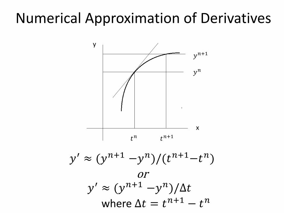
Numerical Approximation of Derivatives
𝑦′ ≈ (𝑦𝑛+1 −𝑦𝑛)/(𝑡𝑛+1−𝑡𝑛)
or𝑦′ ≈ (𝑦𝑛+1 −𝑦𝑛)/Δ𝑡
where Δ𝑡 = 𝑡𝑛+1 − 𝑡𝑛
𝑦𝑛
𝑦𝑛+1
𝑡𝑛 𝑡𝑛+1x
y
Time discretization
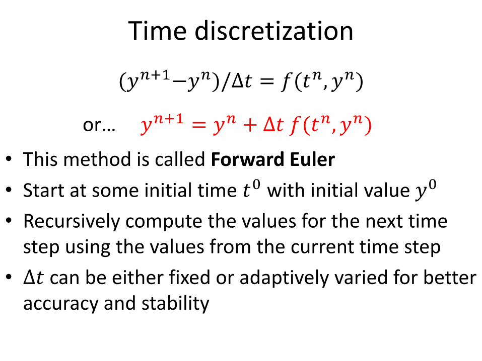
(𝑦𝑛+1−𝑦𝑛)/Δ𝑡 = 𝑓(𝑡𝑛, 𝑦𝑛)
or… 𝑦𝑛+1 = 𝑦𝑛 + Δ𝑡 𝑓(𝑡𝑛, 𝑦𝑛)
• This method is called Forward Euler
• Start at some initial time 𝑡0 with initial value 𝑦0
• Recursively compute the values for the next time step using the values from the current time step
• Δ𝑡 can be either fixed or adaptively varied for better accuracy and stability

Example
Forward Euler: Stability
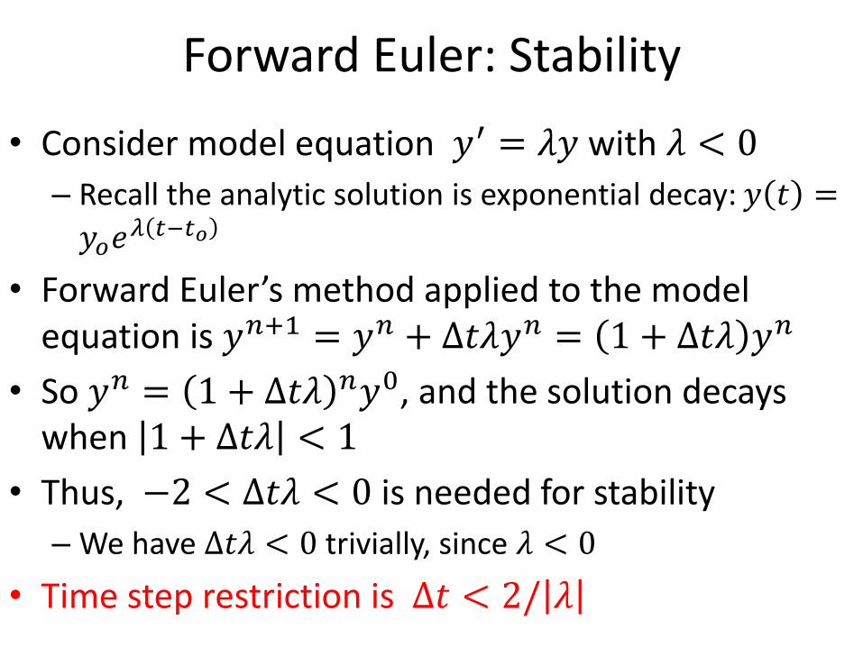
• Consider model equation 𝑦′ = 𝜆𝑦 with 𝜆 < 0
– Recall the analytic solution is exponential decay: 𝑦 𝑡 =
𝑦𝑜𝑒𝜆 𝑡−𝑡𝑜
• Forward Euler’s method applied to the model equation is 𝑦𝑛+1 = 𝑦𝑛 + Δ𝑡𝜆𝑦𝑛 = 1 + Δ𝑡𝜆 𝑦𝑛
• So 𝑦𝑛 = 1 + Δ𝑡𝜆 𝑛𝑦0, and the solution decays when 1 + Δ𝑡𝜆 < 1
• Thus, −2 < Δ𝑡𝜆 < 0 is needed for stability
– We have Δ𝑡𝜆 < 0 trivially, since 𝜆 < 0
• Time step restriction is Δ𝑡 < 2/ 𝜆
Forward Euler: Accuracy
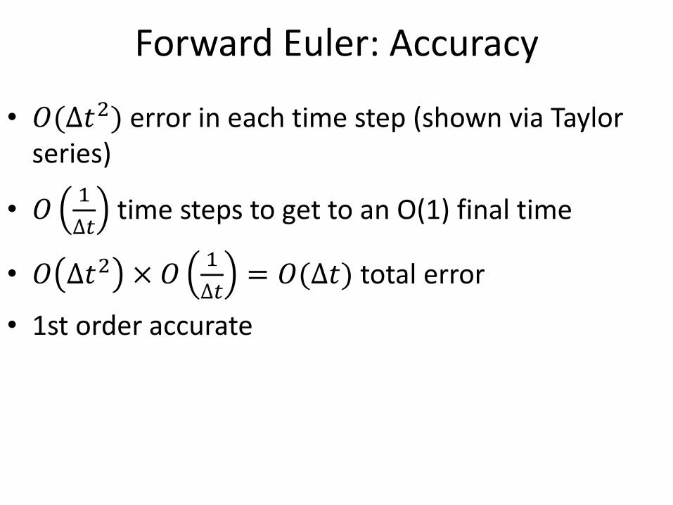
• 𝑂(Δ𝑡2) error in each time step (shown via Taylor series)
• 𝑂1
Δ𝑡time steps to get to an O(1) final time
• 𝑂 Δ𝑡2 × 𝑂1
Δ𝑡= 𝑂(Δ𝑡) total error
• 1st order accurate

MoreNumerical Methods
for ODEs
Runge-Kutta Schemes
• Runge-Kutta (R.K.) builds on Forward Euler (F.E.)
• Achieves better accuracy by predicting solutions using F.E.
– and then uses averaging to get new solutions
• Different prediction and averaging schemes give rise to different R.K. schemes
• 1st order (accurate) R.K. is same as F.E.
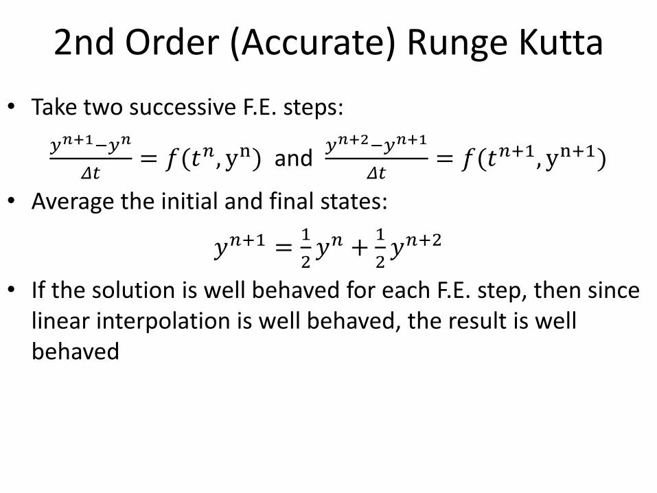
2nd Order (Accurate) Runge Kutta
• Take two successive F.E. steps:
𝑦𝑛+1−𝑦𝑛
𝛥𝑡= 𝑓(𝑡𝑛, yn) and
𝑦𝑛+2−𝑦𝑛+1
𝛥𝑡= 𝑓(𝑡𝑛+1, yn+1)
• Average the initial and final states:
𝑦𝑛+1 =1
2𝑦𝑛 +
1
2𝑦𝑛+2
• If the solution is well behaved for each F.E. step, then since linear interpolation is well behaved, the result is well behaved
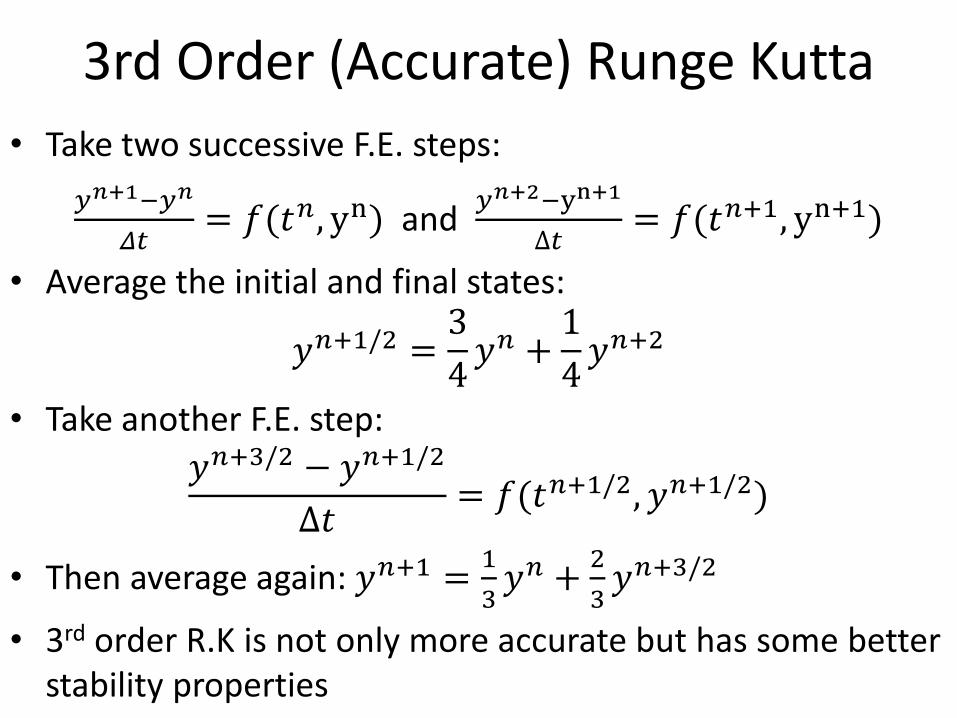
3rd Order (Accurate) Runge Kutta
• Take two successive F.E. steps:
𝑦𝑛+1−𝑦𝑛
𝛥𝑡= 𝑓(𝑡𝑛, yn) and
𝑦𝑛+2−yn+1
Δ𝑡= 𝑓(𝑡𝑛+1, yn+1)
• Average the initial and final states:
𝑦𝑛+1/2 =3
4𝑦𝑛 +
1
4𝑦𝑛+2
• Take another F.E. step:
𝑦𝑛+3/2 − 𝑦𝑛+1/2
Δ𝑡= 𝑓(𝑡𝑛+1/2, 𝑦𝑛+1/2)
• Then average again: 𝑦𝑛+1 =1
3𝑦𝑛 +
2
3𝑦𝑛+3/2
• 3rd order R.K is not only more accurate but has some better stability properties

Even More Numerical Methods
for ODEs

Backward Euler
𝑦𝑛+1 = 𝑦𝑛 + Δ𝑡 𝑓(𝑡𝑛+1, 𝑦𝑛+1)
• Equation is implicit in 𝑦𝑛+1, so generally need to solve a nonlinear equation to find 𝑦𝑛+1
• Newton iteration…. linearize, solve, linearize, solve, etc.
• Some applications (that allow for larger errors) only use one linearize and solve cycle
• Sometimes 𝑓 is already linear in 𝑦
• Accuracy – 1st order (same as forward Euler)
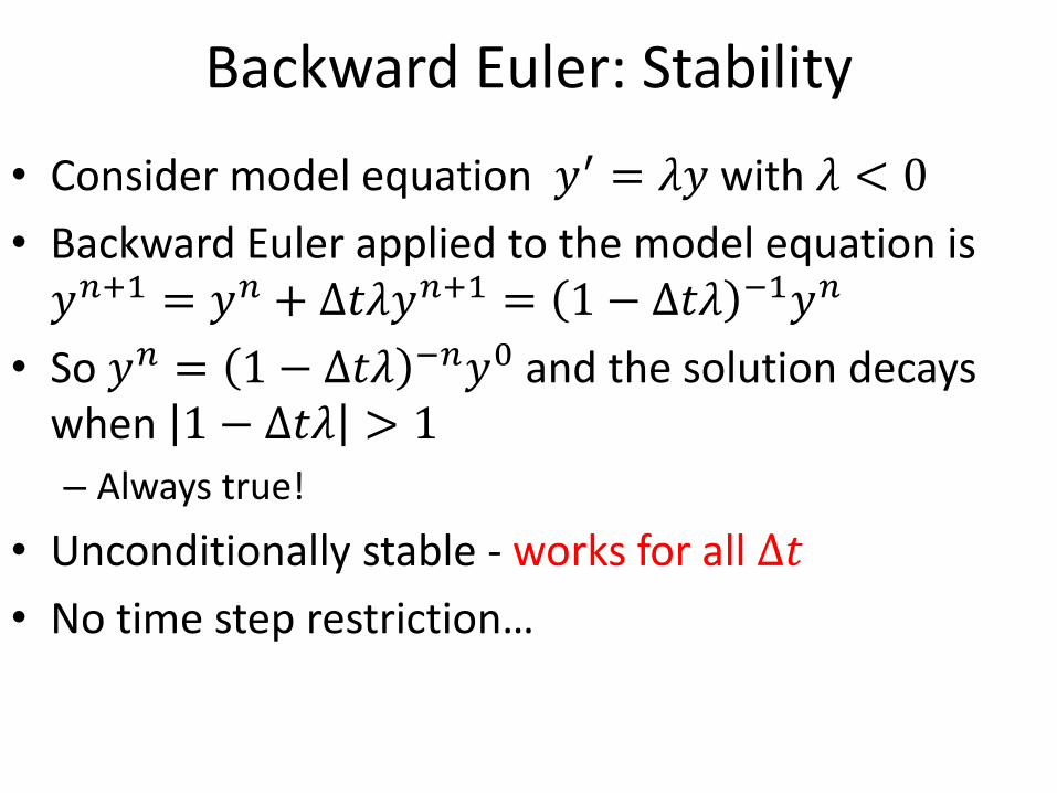
Backward Euler: Stability
• Consider model equation 𝑦′ = 𝜆𝑦 with 𝜆 < 0
• Backward Euler applied to the model equation is𝑦𝑛+1 = 𝑦𝑛 + Δ𝑡𝜆𝑦𝑛+1 = 1 − Δ𝑡𝜆 −1𝑦𝑛
• So 𝑦𝑛 = 1 − Δ𝑡𝜆 −𝑛𝑦0 and the solution decays when 1 − Δ𝑡𝜆 > 1
– Always true!
• Unconditionally stable - works for all Δ𝑡
• No time step restriction…

Backward Euler vs. Forward Euler
• Backward Euler (B.E.) is unconditionally stable
– i.e. one can take very large time steps, whereas Forward Euler (F.E.) requires smaller time steps
• B.E. might excessively damp out the solution, whereas F.E. might blow up (i.e., NaNs)
• Each B.E. time step may be much harder to solve than a F.E. time step
– B.E. is more theoretically challenging and uses more CPU time
• Not always clear which is better…
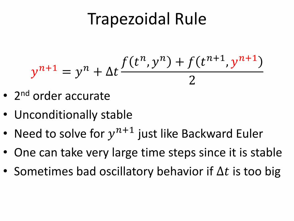
Trapezoidal Rule
𝑦𝑛+1 = 𝑦𝑛 + Δ𝑡𝑓 𝑡𝑛, 𝑦𝑛 + 𝑓 𝑡𝑛+1, 𝑦𝑛+1
2• 2nd order accurate
• Unconditionally stable
• Need to solve for 𝑦𝑛+1 just like Backward Euler
• One can take very large time steps since it is stable
• Sometimes bad oscillatory behavior if Δ𝑡 is too big

The BestNumerical Methods….

Back to our problem…
ሶ𝑥 = 𝑣ሶ𝑣 = 𝐹/𝑚
• We can solve for velocity at one accuracy level lower than for positions (a multivalue method)
• Treating it as a standard system is overkill
• E.g., standard constant acceleration equations
• Ԧ𝑥𝑛+1 = Ԧ𝑥𝑛 + Δ𝑡 Ԧ𝑣𝑛 +Δ𝑡2
2Ԧ𝑎𝑛 piecewise quadratic
position
• Ԧ𝑣𝑛+1 = Ԧ𝑣𝑛 + Δ𝑡 Ԧ𝑎𝑛 piecewise linear velocity
• Ԧ𝑎𝑛+1 = Ԧ𝑎𝑛 piecewise constant acceleration (constant from time n to just before time n+1)
Newmark Methods
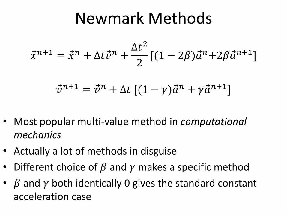
Ԧ𝑥𝑛+1 = Ԧ𝑥𝑛 + Δ𝑡 Ԧ𝑣𝑛 +Δ𝑡2
2[(1 − 2𝛽) Ԧ𝑎𝑛+2𝛽 Ԧ𝑎𝑛+1]
Ԧ𝑣𝑛+1 = Ԧ𝑣𝑛 + Δ𝑡 [(1 − 𝛾) Ԧ𝑎𝑛 + 𝛾 Ԧ𝑎𝑛+1]
• Most popular multi-value method in computational mechanics
• Actually a lot of methods in disguise
• Different choice of 𝛽 and 𝛾 makes a specific method
• 𝛽 and 𝛾 both identically 0 gives the standard constant acceleration case
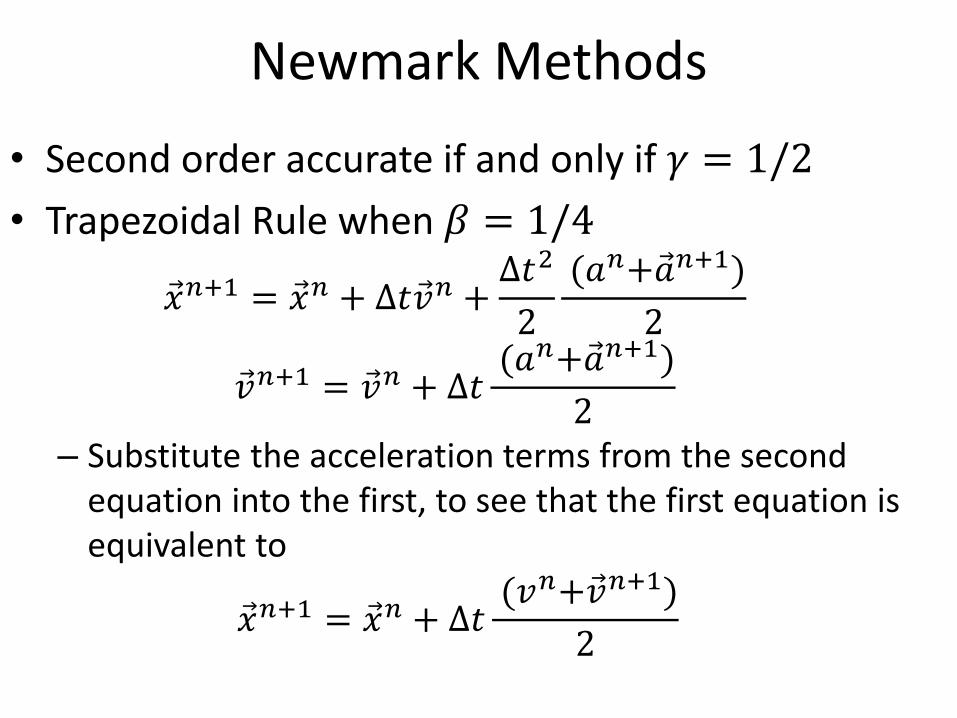
Newmark Methods
• Second order accurate if and only if 𝛾 = 1/2
• Trapezoidal Rule when 𝛽 = 1/4
Ԧ𝑥𝑛+1 = Ԧ𝑥𝑛 + Δ𝑡 Ԧ𝑣𝑛 +Δ𝑡2
2
(𝑎𝑛+Ԧ𝑎𝑛+1)
2
Ԧ𝑣𝑛+1 = Ԧ𝑣𝑛 + Δ𝑡(𝑎𝑛+Ԧ𝑎𝑛+1)
2– Substitute the acceleration terms from the second
equation into the first, to see that the first equation is equivalent to
Ԧ𝑥𝑛+1 = Ԧ𝑥𝑛 + Δ𝑡(𝑣𝑛+Ԧ𝑣𝑛+1)
2

A Newmark Method…
1. Ԧ𝑣𝑛+1/2 = Ԧ𝑣𝑛 +Δ𝑡
2Ԧ𝑎(𝑡𝑛, Ԧ𝑥𝑛, Ԧ𝑣𝑛+1/2)
2. Modify Ԧ𝑣𝑛+1/2 in some cases, e.g. collisions
3. Ԧ𝑥𝑛+1 = Ԧ𝑥𝑛 + Δ𝑡 Ԧ𝑣𝑛+1/2
4. Ԧ𝑣𝑛+1 = Ԧ𝑣𝑛+1/2 +Δ𝑡
2Ԧ𝑎 𝑡𝑛+1, Ԧ𝑥𝑛+1, Ԧ𝑣𝑛+1
5. Modify Ԧ𝑣𝑛+1 in some cases, e.g. collisions

Implicit Solve
• Steps 1 and 4 are implicit in Ԧ𝑣𝑛+1/2 and Ԧ𝑣𝑛+1
respectively
• Typically the equations are linear in v, so we onlyneed to solve a single matrix system
• The matrix is generally symmetric positive definite (SPD) and we can use fast solvers such as conjugate gradients (CG) for solving the system
• Note that in the first step we are using Ԧ𝑥𝑛 instead of Ԧ𝑥𝑛+1/2
– The equations are typically highly nonlinear in x

Question #3
LONG FORM:• Tell me everything about…. Nvm, have a nice day!
SHORT FORM:• ☺


