1

Vivek Varadarajan and Jeffrey KrolikDuke University

Department of Electrical and Computer EngineeringDurham, NC 27708, USA

Sponsored by ONR Code 321 under the Uncertainty DRI

Acoustical Society of America Meeting Fall 2005

Passive Sonar Detection Performance Prediction of a Moving Source in an Uncertain

Environment

2

Sonar Detection in an Uncertain Environment

OBJECTIVE: To nowcast passive sonar detection performance using a moving source of opportunity in an uncertain channel and noise field.

BACKGROUND:

• Estimation of array gain (AG) and transmission loss (TL) is critical to predicting detection performance.

• Performance prediction typically performed using environmental measurements and acoustic models to predict TL and AG.

• A source-of-opportunity (SO) can also be used to estimate AG and TL but multipathpropagation and source motion complicates this measurement because of the resulting space-time signal wavefront fluctuations.

• Nowcasting performance using a SO can be used to validate model-based performance prediction.

• In this work, a moving SO is used to nowcast detection performance when both the ocean environment and noise covariance are uncertain.

3

Detection Performance Characterization

• Detection performance characterized by receiver operating characteristic (ROC) as a function of output SNR, time-bandwidth product, noise training data, and degree of signal wavefront uncertainty.

• The sonar equation summarizes the ROC as the output SNR (i.e. detection threshold, DT) needed to achieve a specific probability of detection (PD) and false alarm (PFA).

• A more complete description is given by PD vs. SNR for fixed PFA which, in principle, can be mapped to PD vs. Range.

• Accurate performance nowcastingstarts with being able to predict the output SNR from a hypothesized target.

Example PD vs. SNR for PFA=0.1

This curve bounded by optimal detectorsmatched to degree of environmental uncertainty

4

Estimating Output Signal-to-Noise Ratio

• In an uncertain waveguide, the M-sensor passive detection problem is given by:

• Output SNR is defined by where is the unknown covariance matrix of the zero-mean Gaussian noise.

• Equivalently, in terms of the sonar equation, SNR = SL – TL + AG – NL.

• Prediction of output SNR requires knowledge of the signal wavefront, noise covariance, and source level, all of which uncertain.

• Estimates of the unknown Gaussian noise covariance can, in principle, be obtained from neighboring times/frequencies/bearings. Target source level can be hypothesized based on a priori knowledge.

• But TL and AG must be estimated from models and/or sources of opportunity.

2 1H HSNR s a U R Uaη

−=

( )γ θθ φ φ

θ γ

− −= =sin sin

s

where [ ( )] ( ) ,[ ( , )] ( ) , are

unknown amplitudes, , , are source bearing, range, depth, and is array tilt.

l s l sjk md jk rs ml l m s s l l s l s n

s s

U z e a r z z k r e s

r z

η θ η= +=o 1H ( )H : versus : n n n s nn x s U ax

η η η= ( )Hn nR E

5

• Transmission loss can be determined by taking the ratio of the signal power of the beamformer output in the SO direction to the source level.

• Sounds simple. But what’s the signal wavefront?

• Assuming SO emits a set of narrowband components, we estimate SO wavefrontat each tonal by computing the dominant eigenvector of the data covariance with maximum projection onto hypothesized SO wavefront (e.g. plane-wave in SO direction).

• The maximum averaging time available to form a nearly rank-one signal covariance matrix is limited by how long the SO remains within a single beam.

• Using the estimated signal wavefront, , the beamformer output may be used to obtain an instantaneous signal power estimate for snapshot n and frequency bin k:

where is the assumed known SO source level and e.g.

• But is this estimate of TL statistically stable?

Estimating TL from a Source of Opportunity

ˆsv

( )22

ˆˆ( , ) ( , ) ,sk SO v k kTL n w n x nω σ ω ω+=

2SOσ

1 1ˆ ˆˆ ˆ ˆ ˆ( , )sv k s s sw n R v v R vη ηω − + −=

6

Short-Time Transmission Loss Fluctuations

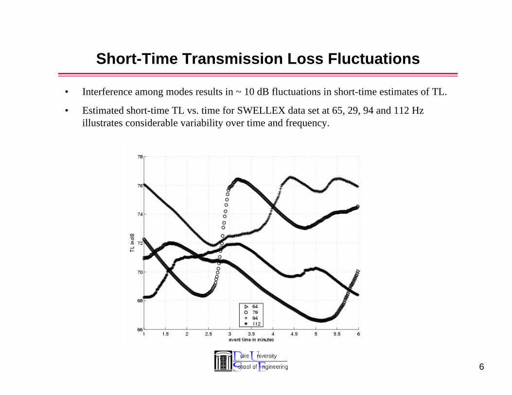
• Interference among modes results in ~ 10 dB fluctuations in short-time estimates of TL.

• Estimated short-time TL vs. time for SWELLEX data set at 65, 29, 94 and 112 Hz illustrates considerable variability over time and frequency.

7

Obtaining Statistically Stable TL and AG Estimates

2max ( ) s m n s

rtv k k vδ πδ = =

−

2

max m nk k r

πδω

ω ω

=∂ ∂⎛ ⎞−⎜ ⎟∂ ∂⎝ ⎠

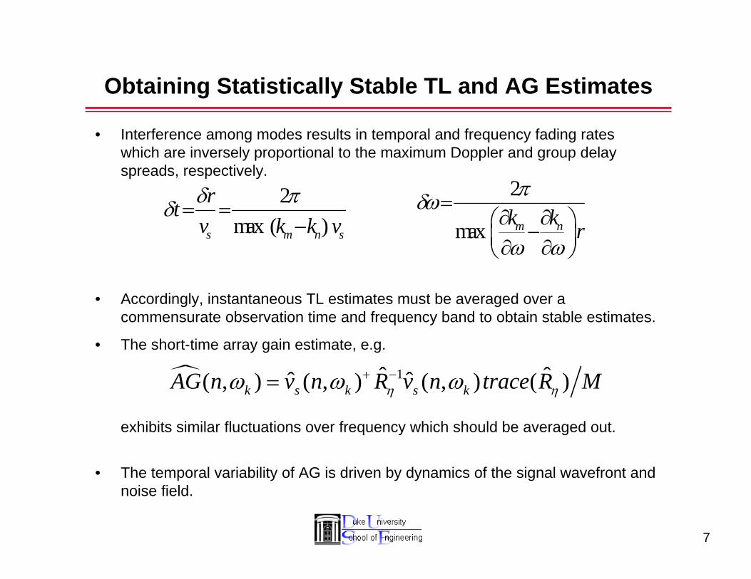
• Interference among modes results in temporal and frequency fading rates which are inversely proportional to the maximum Doppler and group delay spreads, respectively.

• Accordingly, instantaneous TL estimates must be averaged over a commensurate observation time and frequency band to obtain stable estimates.

• The short-time array gain estimate, e.g.

exhibits similar fluctuations over frequency which should be averaged out.

• The temporal variability of AG is driven by dynamics of the signal wavefront and noise field.

1ˆ ˆˆ ˆ( , ) ( , ) ( , ) ( )k s k s kAG n v n R v n trace R Mη ηω ω ω+ −=

8

Adaptive Multi-rank CFAR Detection

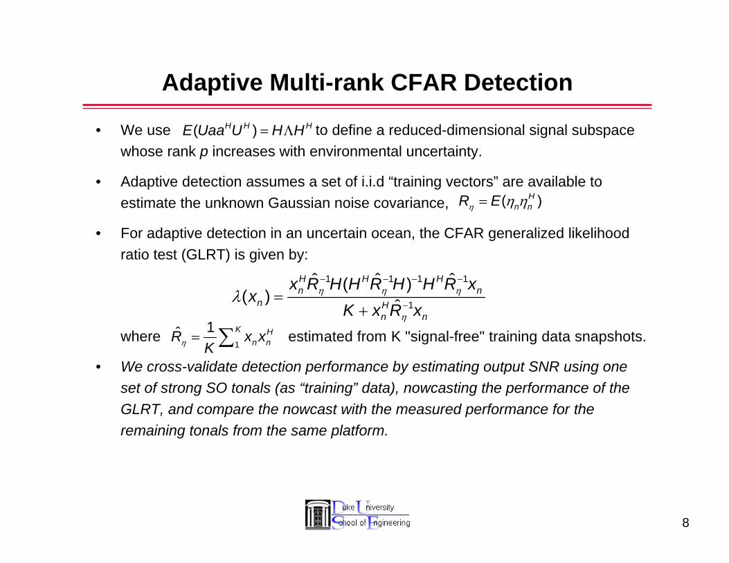
• We use to define a reduced-dimensional signal subspace whose rank p increases with environmental uncertainty.

• Adaptive detection assumes a set of i.i.d “training vectors” are available to estimate the unknown Gaussian noise covariance,

• For adaptive detection in an uncertain ocean, the CFAR generalized likelihood ratio test (GLRT) is given by:

where

• We cross-validate detection performance by estimating output SNR using one set of strong SO tonals (as “training” data), nowcasting the performance of the GLRT, and compare the nowcast with the measured performance for the remaining tonals from the same platform.

= Λ( )H H HE Uaa U H H

η η η= ( )Hn nR E

1 1 1 1

1

ˆ ˆ ˆ( )( ) ˆ

H H Hn n

n Hn n

x R H H R H H R xx

K x R xη η η

η

λ− − − −

−=

+

1

1ˆ estimated from K "signal-free" training data snapshots.K Hn nR x x

Kη = ∑

9

Analytic Probability of Detection vs. Output SNR

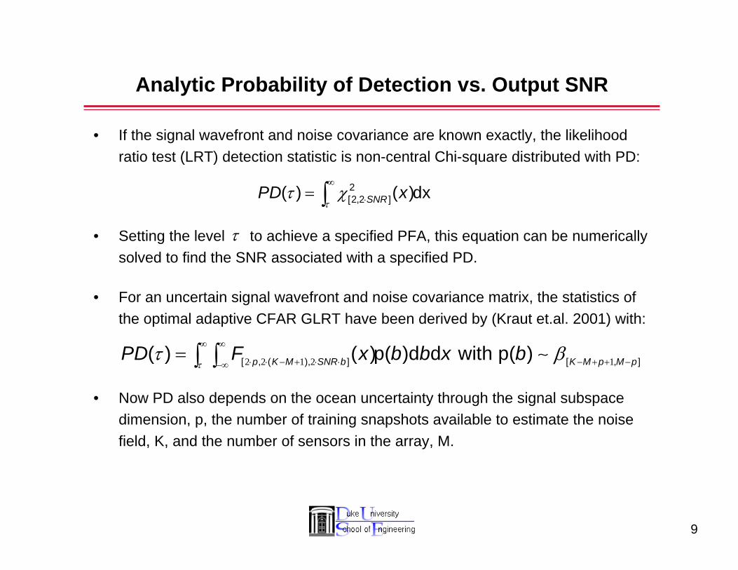
• If the signal wavefront and noise covariance are known exactly, the likelihood ratio test (LRT) detection statistic is non-central Chi-square distributed with PD:

• Setting the level to achieve a specified PFA, this equation can be numerically solved to find the SNR associated with a specified PD.

• For an uncertain signal wavefront and noise covariance matrix, the statistics of the optimal adaptive CFAR GLRT have been derived by (Kraut et.al. 2001) with:

• Now PD also depends on the ocean uncertainty through the signal subspace dimension, p, the number of training snapshots available to estimate the noise field, K, and the number of sensors in the array, M.

2 2 1 2 1[ , ( ), ] [ , ]( ) ( )p( )d d with p( )p K M SNR b K M p M pPD F x b b x bτ

τ β∞ ∞

⋅ ⋅ − + ⋅ ⋅ − + + −−∞= ∫ ∫ ∼

2[2,2 ]( ) ( )dxSNRPD x

ττ χ

∞

⋅= ∫τ

10

Cross-Validating Nowcast Performance with Real Data

• Block diagram of cross-validation procedure involving training and test tones from source of opportunity.

Estimate TLand AG

Source Levels

SO TrainingTone Snapshots

Estimate OutputSNR of Test

Tones

NumericallyCompute ROC’s

vs. SNR, K, p

K Noise-OnlySnapshots

Estimate NoiseCovariance

Adaptive GLRTDetector

SO TestSnapshots

Estimate ROC’sfrom Test Data

Compare

11

Detection Nowcasting with SWellEx-96 Data

• The SWellEx-96 Experiment was conducted between May 10 and 18, 1996, approximately 12 km from the tip of Point Loma near San Diego, California.

• The source of opportunity was a towed source at a depth of 54 meter,and transmitted a set of tones at different power levels and frequencies as below

49 64 79 94 112 130 148 166 201 235 283 338 388 <-- 158 dB52 67 82 97 115 133 151 169 204 238 286 341 391 <-- 132 dB55 70 85 100 118 136 154 172 207 241 289 344 394 <-- 128 dB58 73 88 103 121 139 157 175 210 244 292 347 397 <-- 124 dB61 76 91 106 124 142 160 178 213 247 295 350 400 <-- 120 dB.

• A horizontal array, which is approximately linear, and of length 240 meter was used to collect the data. The number of elements in the array i.e. M is 27. .

• The Kraken normal mode program was used to compute an estimate of the integration time and bandwidth needed to average the fluctuations in the transmission loss and array gain.

• Transmission loss and array gain are computed for each frequency and time, using tones at the power level of 158 dB.

• The transmission loss and array gain are averaged over a band .

• Transmission loss is further averaged over the integration time

25Hzδω >

30sec.tδ >

12

Swell-Ex 96 S5 Event Bearing Time Record

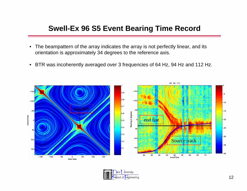
• The beampattern of the array indicates the array is not perfectly linear, and its orientation is approximately 34 degrees to the reference axis.

• BTR was incoherently averaged over 3 frequencies of 64 Hz, 94 Hz and 112 Hz.

end fire

Source track

end fire

13

Ambient Noise Power Variability

• The input noise power variation over time is shown below. Noise frequencies were 5 Hz apart, on either side of the 4 different signal frequencies, i.e 64 Hz, 79 Hz, 94 Hz, 112 Hz.128 snapshots with 50 % over lap was used to compute the noise correlation matrix.

14

Estimated Output SNR and Probability of Detection

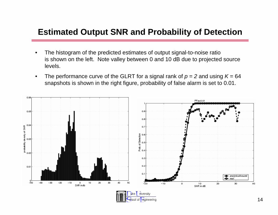
• The histogram of the predicted estimates of output signal-to-noise ratiois shown on the left. Note valley between 0 and 10 dB due to projected source levels.

• The performance curve of the GLRT for a signal rank of p = 2 and using K = 64 snapshots is shown in the right figure, probability of false alarm is set to 0.01.

15

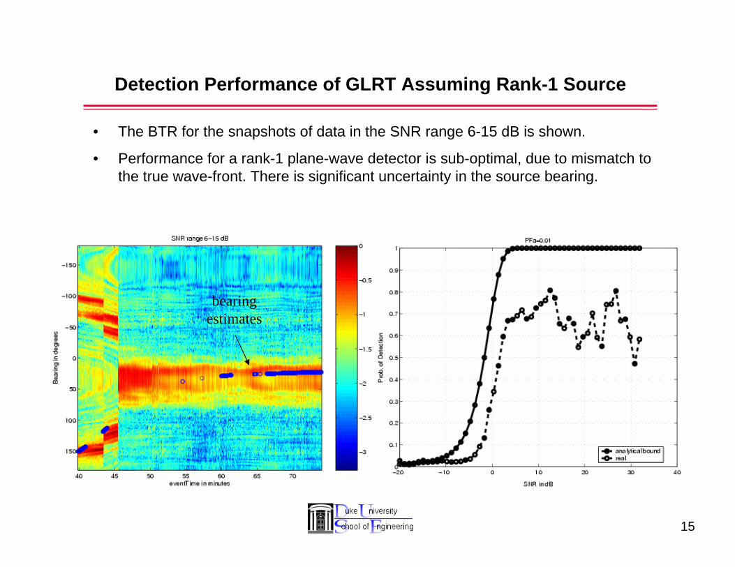
Detection Performance of GLRT Assuming Rank-1 Source

• The BTR for the snapshots of data in the SNR range 6-15 dB is shown.

• Performance for a rank-1 plane-wave detector is sub-optimal, due to mismatch to the true wave-front. There is significant uncertainty in the source bearing.

bearing estimates

16

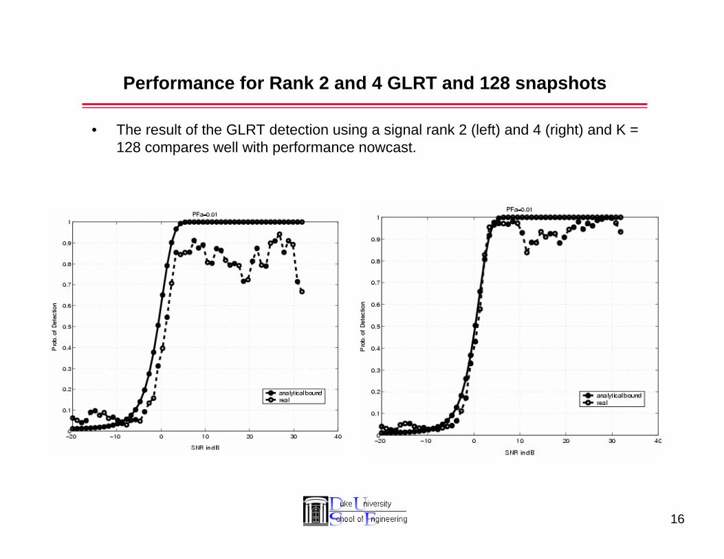
Performance for Rank 2 and 4 GLRT and 128 snapshots

• The result of the GLRT detection using a signal rank 2 (left) and 4 (right) and K = 128 compares well with performance nowcast.

17

Conclusions

• Nowcasts of detection performance using sources-of-opportunity could facilitate in situ validation environmental model-based performance predictions.

• Estimates of transmission loss (TL) and array gain (AG) from a source of opportunity can be used to predict output SNR for a target of interest.

• Statistically stable TL and AG estimates achieved by using eigenvector-based signal wavefront estimates and averaging over time-frequency fluctuations induced by differential multipath Doppler and delay spread.

• Given predicted output SNR, signal rank (p), and noise training data support (K) quasi-analytic calculation of ROC can be rapidly computed for adaptive multi-rank CFAR GLRT detector.

• We have cross-validated nowcasts of detection performance using training tones to predict TL and AG and test tones to form the GLRT detection statistic from a moving source.

• Results with SWELLEX-96 data show excellent agreement with nowcastassuming appropriate signal rank and noise covariance sample support.