Computational Discovery of Scientific Models: Guiding Search with Knowledge and Data. Pat Langley Department of Computer Science University of Auckland Private Bag 92019 Auckland 1142 NZ. - PowerPoint PPT Presentation
Thanks to K. Arrigo, G. Bradshaw, S. Borrett, W. Bridewell, S. Dzeroski, H. Simon, L. Todorovski, and J. Zytkow for their contributions to this research, which was partly funded by NSF Grant No. IIS-0326059 and ONR Grant No. Pat Langley Department of Computer Science University of Auckland Private Bag 92019 Auckland 1142 NZ Computational Discovery of Scientific Models: Guiding Search with Knowledge and Data
Transcript
Thanks to K. Arrigo, G. Bradshaw, S. Borrett, W. Bridewell, S. Dzeroski, H. Simon, L. Todorovski, and J. Zytkow for their contributions to this research, which was partlyfunded by NSF Grant No. IIS-0326059 and ONR Grant No. N00014-11-1-0107.
Pat Langley
Department of Computer ScienceUniversity of Auckland
Private Bag 92019Auckland 1142 NZ
Computational Discovery of Scientific Models: Guiding Search with Knowledge and Data
The Scientific Enterprise
Systematic collection and analysis of observations
Formal statement of theories, laws, and models
Use of the latter to explain and predict the former
Use of observations to evaluate theorized structures
Science is a unique collection of activities distinguished by some distinctive characteristics:
Moreover, science can apply these ideas to any area of enquiry, in principle even to science itself.
Philosophy of Science
character of scientific observations and experiments
structure of scientific theories, laws, and models
nature of scientific explanations and predictions
evaluation of scientific theories, models, and laws
One discipline – philosophy of science – has studied science itself since the 19th Century, including the:
However, philosophers of science have typically avoided one important topic: scientific discovery.
Philosophers largely ignored scientific discovery, believing it to be immune to logical analysis. Popper (1934) wrote:
The initial stage, the act of conceiving or inventing a theory, seems to me neither to call for logical analysis nor to be susceptible of it … My view may be expressed by saying that every discovery contains an ‘irrational element’, or ‘a creative intuition’…
He was not alone in this view. Hempel and many others believed discovery was inherently irrational and beyond understanding.
However, advances made by two fields – cognitive psychology and artificial intelligence – in the 1950s suggested otherwise.
Mystical Views of Scientific Discovery
Scientific Discovery as Problem Solving
Search through a space of connected problem states
Generated from earlier states by mental operators
Guided by heuristics that keep the search tractable
Simon (1966) offered another view – that scientific discovery is a variety of problem solving that involves:
Heuristic search had been implicated in many cases of human problem solving, such as proving theorems and playing chess.
This idea offered a powerful new approach to understanding the rational character of scientific discovery.
But it also suggested ways to automate this mysterious process.
Heuristic Search in a Problem Space
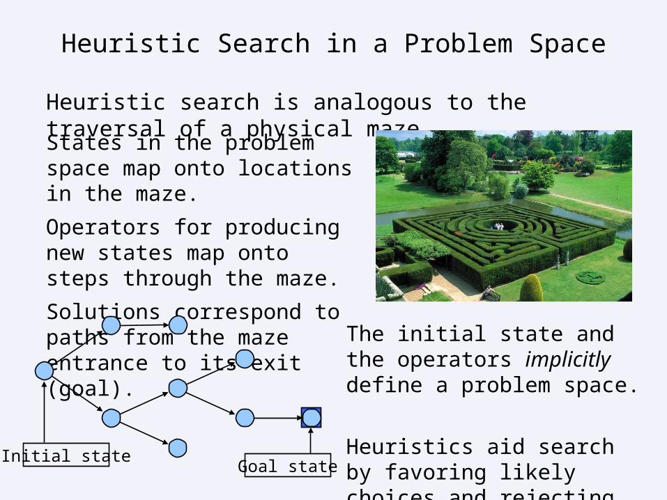
Heuristic search is analogous to the traversal of a physical maze.
The initial state and the operators implicitly define a problem space.
Heuristics aid search by favoring likely choices and rejecting others to make solution finding tractable.
States in the problem space map onto locations in the maze.
Operators for producing new states map onto steps through the maze.
Solutions correspond to paths from the maze entrance to its exit (goal).
Initial stateGoal state
An Early Response
Carried out search in a problem space of theoretical terms;
Using operators that combined old terms into new ones;
Guided by heuristics that noted regularities in data; and
Applied these recursively to formulate higher-level relations.
For my CMU dissertation research, I adapted Simon’s ideas on scientific discovery, developing a computer program that:
The result was Bacon, an early AI system that rediscovered laws from the history of physics and chemistry.
I named the system after Sir Francis Bacon because it adopted a data-driven approach to discovery.
Bacon on Kepler’s Third Law
D
ABC
d/pp
16.69
1.773.577.16
1.48
3.202.431.96
d2/p
36.46
18.1521.0427.40
d3/p2
53.89
58.1551.0653.61
moon d
24.67
5.678.67
14.00
The Bacon system carried out heuristic search, through a space of numeric terms, looking for constants and linear relations.
This table shows its progression from the distance and period of Jupiter’s moons to a term with nearly constant value.
Bacon on the Ideal Gas Law
Bacon rediscovered the ideal gas law, PV = aNT + bN, in three stages, each at a different level of description.
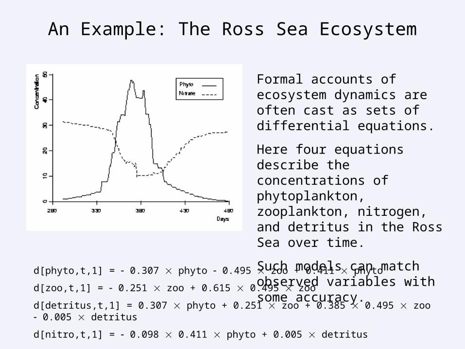
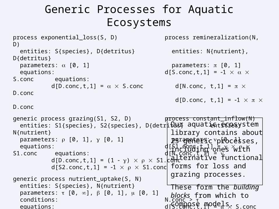
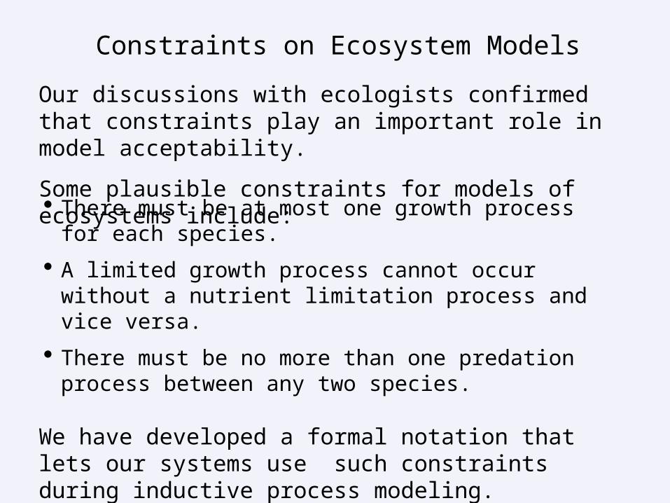
As phytoplankton uptakes nitrogen, its concentration increases and the nitrogen decreases. This continues until the nitrogen is exhausted, which leads to a phytoplankton die off. This produces detritus, which gradually remineralizes to replenish nitrogen. Zooplankton grazes on phytoplankton, which slows the latter’s increase and also produces detritus.
As phytoplankton uptakes nitrogen, its concentration increases and the nitrogen decreases. This continues until the nitrogen is exhausted, which leads to a phytoplankton die off. This produces detritus, which gradually remineralizes to replenish nitrogen. Zooplankton grazes on phytoplankton, which slows the latter’s increase and also produces detritus.
As phytoplankton uptakes nitrogen, its concentration increases and the nitrogen decreases. This continues until the nitrogen is exhausted, which leads to a phytoplankton die off. This produces detritus, which gradually remineralizes to replenish nitrogen. Zooplankton grazes on phytoplankton, which slows the latter’s increase and also produces detritus.
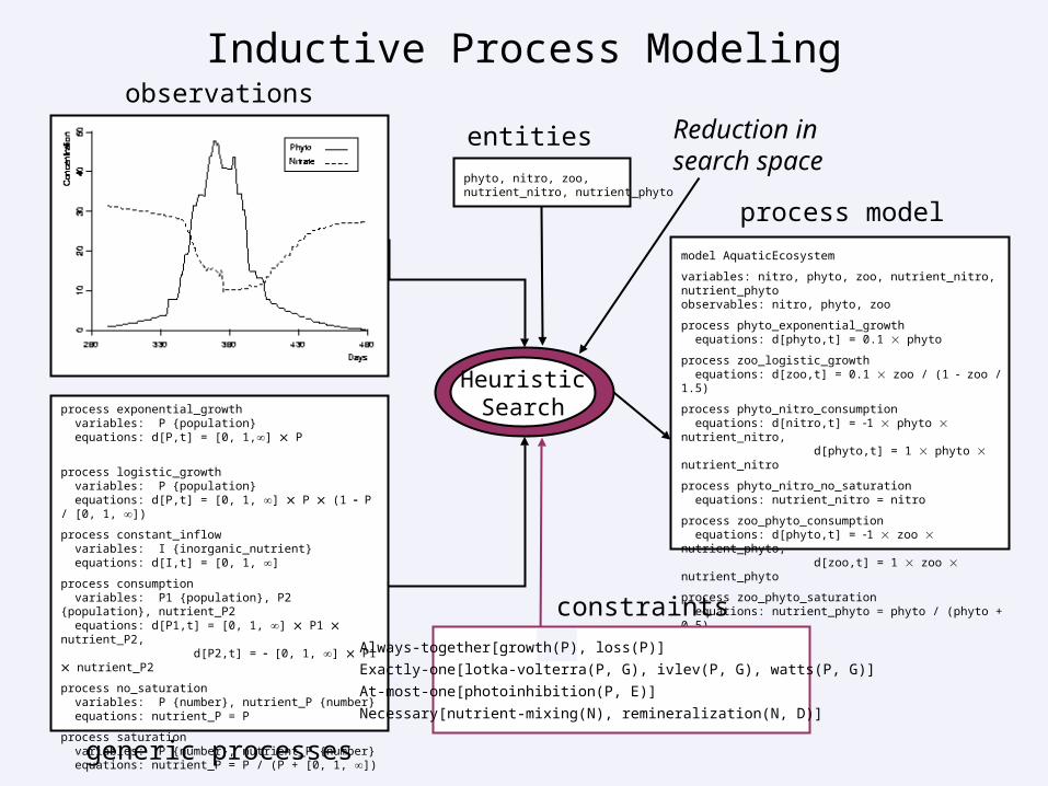
Encodes modular constraints on process combinations
Uses these constraints to eliminate unacceptable models
Reduces search through the model space, which
Leads to far more efficient model construction
Produces little or no increase in generalization error
Improves the comprehensibility of generated models
Our extended framework for the discovery of process models:
The resulting systems are more robust in their ability to induce process models (Bridewell & Langley, TopiCS, 2010).
Discovering Constraints
Uses inductive process modeling to generate a set of models;
Separates these into accurate and inaccurate model structures;
Describes each model structure in terms of relational literals;
Learns relational rules that can distinguish the two classes;
Transforms the rules into constraints on model structures; and
Uses these constraints to guide search on future modeling tasks.
In other recent work (Todorovski et al., AAAI-2012), we have developed a system that:
Experiments suggests this produces a tenfold speedup on novel modeling tasks with little or no loss in accuracy.
Directions for Future Research
apply approach to new data sets (oceanography, physiology)
develop more efficient methods for fitting model parameters
extend the framework to partial differential equation models
design mechanisms for inducing new generic processes
handle discovery of complex models with many variables
embed these abilities in a PROMETHEUS-like environment
Despite the progress to date, we need further work in order to:
Together, these will make constraint-guided inductive process modeling a more robust approach to scientific explanation.
Summary Remarks
Incorporates a formalism that is familiar to many scientists
Utilizes two kinds of background knowledge about the domain
Produces meaningful results from moderate amounts of data
Generates models that explain, not just describe, observations
Closes the loop between using and learning process constraints
Inductive process modeling is a novel and promising approach to discovering scientific models that:
Although work on this topic has focused on ecological modeling, the key ideas extend to other domains.
For more information, see http://www.isle.org/process/ .
eScience and Discovery Informatics
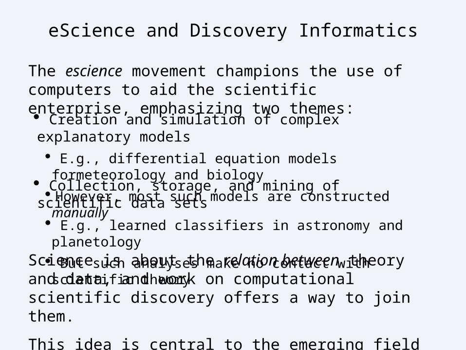
Creation and simulation of complex explanatory models E.g., differential equation models formeteorology and biology
However, most such models are constructed manually
The escience movement champions the use of computers to aid the scientific enterprise, emphasizing two themes:
Science is about the relation between theory and data, and work on computational scientific discovery offers a way to join them.
This idea is central to the emerging field of discovery informatics.
Collection, storage, and mining of scientific data sets
E.g., learned classifiers in astronomy and planetology
But such analyses make no contact with scientific theory
Big Data and Scientific Discovery
Scaling to large and heterogeneous data sets
Scaling to large and complex scientific models
Scaling to large spaces of candidate models
Digital collection and storage have led to rapid growth of data in many areas.
The big data movement seeks to capitalize on this content, but, in science at least, must address three distinct issues:
Handling large data sets has been widely studied and poses the fewest challenges.
We need more work on the last two issues, for which the methods of computational scientific discovery are well suited.
Concluding Remarks
Scientific discovery does not involve any mystical or irrational elements; we can study and even partially automate it.
Our explanation of this fascinating set of processes relies on:
Carrying out search through a space of laws or models;
Utilizing operators for generating structures and parameters;
Guiding search by data and by knowledge about the domain.
Work in this framework discovers laws and models stated in the formalisms and concepts familiar to scientists.
This paradigm has already started to aid the scientific enterprise, and its importance will only grow with time.
Publications on Computational Scientific Discovery
Bridewell, W., & Langley, P. (2010). Two kinds of knowledge in scientific discovery. Topics in Cognitive Science, 2, 36–52.
Bridewell, W., Langley, P., Todorovski, L., & Dzeroski, S. (2008). Inductive process modeling. Machine Learning, 71, 1-32.
Bridewell, W., Sanchez, J. N., Langley, P., & Billman, D. (2006). An interactive environment for the modeling and discovery of scientific knowledge. International Journal of Human-Computer Studies, 64, 1099-1114.
Dzeroski, S., Langley, P., & Todorovski, L. (2007). Computational discovery of scientific knowledge. In S. Dzeroski & L. Todorovski (Eds.), Computational discovery of communicable scientific knowledge. Berlin: Springer.
Langley, P. (2000). The computational support of scientific discovery. International Journal of Human-Computer Studies, 53, 393–410.
Langley, P., Simon, H. A., Bradshaw, G. L., & Zytkow, J. M. (1987). Scientific discovery: Computational explorations of the creative processes. Cambridge, MA: MIT Press.
Langley, P., & Zytkow, J. M. (1989). Data-driven approaches to empirical discovery. Arti-ficial Intelligence, 40, 283–312.
Todorovski, L., Bridewell, W., & Langley, P. (2012). Discovering constraints for inductive process modeling. Proceedings of the Twenty-Sixth AAAI Conference on Artificial Intelligence. Toronto: AAAI Press.
In Memoriam
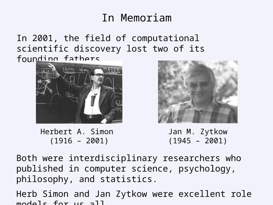
Herbert A. Simon (1916 – 2001)
In 2001, the field of computational scientific discovery lost two of its founding fathers.
Both were interdisciplinary researchers who published in computer science, psychology, philosophy, and statistics.
Herb Simon and Jan Zytkow were excellent role models for us all.