HAL Id: hal-00733789 https://hal.archives-ouvertes.fr/hal-00733789 Submitted on 22 Jan 2013 HAL is a multi-disciplinary open access archive for the deposit and dissemination of sci- entific research documents, whether they are pub- lished or not. The documents may come from teaching and research institutions in France or abroad, or from public or private research centers. L’archive ouverte pluridisciplinaire HAL, est destinée au dépôt et à la diffusion de documents scientifiques de niveau recherche, publiés ou non, émanant des établissements d’enseignement et de recherche français ou étrangers, des laboratoires publics ou privés. Path-Following Algorithms and Experiments for an Unmanned Surface Vehicle Marco Bibuli, Gabriele Bruzzone, Massimo Caccia, Lionel Lapierre To cite this version: Marco Bibuli, Gabriele Bruzzone, Massimo Caccia, Lionel Lapierre. Path-Following Algorithms and Experiments for an Unmanned Surface Vehicle. Journal of Field Robotics, Wiley, 2009, 26, pp.669-688. 10.1002/rob.20303. hal-00733789
Transcript
HAL Id: hal-00733789https://hal.archives-ouvertes.fr/hal-00733789
Submitted on 22 Jan 2013
HAL is a multi-disciplinary open accessarchive for the deposit and dissemination of sci-entific research documents, whether they are pub-lished or not. The documents may come fromteaching and research institutions in France orabroad, or from public or private research centers.
L’archive ouverte pluridisciplinaire HAL, estdestinée au dépôt et à la diffusion de documentsscientifiques de niveau recherche, publiés ou non,émanant des établissements d’enseignement et derecherche français ou étrangers, des laboratoirespublics ou privés.
Path-Following Algorithms and Experiments for anUnmanned Surface Vehicle
Marco Bibuli, Gabriele Bruzzone, Massimo Caccia, Lionel Lapierre
To cite this version:Marco Bibuli, Gabriele Bruzzone, Massimo Caccia, Lionel Lapierre. Path-Following Algorithms andExperiments for an Unmanned Surface Vehicle. Journal of Field Robotics, Wiley, 2009, 26, pp.669-688.�10.1002/rob.20303�. �hal-00733789�
This paper addresses the problem of path-following in two-dimensional space for
underactuated unmanned surface vehicles (USVs), defining a set of guidance laws
at kinematic level. The proposed nonlinear Lyapunov-based control law yields con-
vergence of the path following error coordinates to zero. Furthermore, the introduc-
tion of a virtual controlled degree of freedom for the target to be followed on the
path removes singularity behaviors present in other guidance algorithms proposed
in the literature. Some heuristic approaches are then proposed to face the problem
of speed of advance adaptation based on path curvature measurement and steering
action prediction. Finally a set of experimental results of all the proposed guidance
laws, carried out with the Charlie USV, demonstrate the feasibility of the proposed
approach and the performance improvements, in terms of precision in following
the reference path and transient reduction, obtained introducing speed adaptation
heuristics.
1 Introduction
In the last fifteen years a large number of Unmanned Surface Vehicles (USVs) have been developed
for a large set of applications such as environmental monitoring and sampling, coastal protection,
bathymetric surveys, support for Autonomous Underwater Vehicles (AUVs) operations.
Some examples are given by the family of USVs at the MIT AUV Lab (Manley et al., 2000) (Ben-
jamin and Curcio, 2004); the flotilla of autonomous marine vehicles, such as Delfim and Caravela,
at the Lisbon IST-ISR Dynamical System and Ocean Robotics Laboratory (Pascoal and et al.,
2000) (Alves et al., 1999); the Charlie USV originally developed by CNR-ISSIA Genova for sea
surface microlayer sampling and then applied to restricted water operations (Caccia et al., 2007);
the ROAZ autonomous surface vehicles developed by the Instituto Superior de Engenharia do
Porto also devoted to search and rescue support (Martins et al., 2006); and the catamaran Springer
developed by the Plymouth University to monitor and track water pollution (Xu et al., 2006).
On the military side, the project SWIMS, i.e. shallow water influence mine sweeping system,
by QinetiQ Ltd successfully demonstrated a conversion kit able to convert standard RIBs (rigid
inflatable boats) in remotely controlled ones, during the second Gulf War (Cornfield and Young,
2006). After that, research mainly focuses on the development and integration of sensors for over-
the-water obstacle detection and avoidance. Examples are given by the testbed developed at SSC
San Diego (Ebken et al., 2005), based on the Bombardier SeaDoo Challenger 2000, and the Israeli
Protector USV (Pro, ), equipped with radar and advanced electro-optical devices.
For major details about USV technology, the reader can refer to (Caccia, 2006) and (Manley, 2008).
In this context, the existing prototype USVs, typically not equipped with side thrusters and thus
under-actuated, are required to perform tasks which need increasing manoeuvring accuracy, mov-
ing, for instance, from the goal of executing an integral sampling in a relatively large area to the
aim of reconstructing a very precise bathymetry of a littoral zone.
Generally speaking, the problems related to motion control of UMVs are classified in the literature
into three basic groups:
• point stabilization: the goal is to stabilize the vehicle zeroing the position and orientation
error with respect to a given target point, with a desired orientation. The goal cannot be
achieved with smooth or continuous state-feedback control laws, when the vehicle has
nonholonomic constraints; in this case, approaches like smooth time-varying control laws
and discontinuous and hybrid feedback laws have been proposed;
• trajectory tracking: the vehicle is required to track a time-parameterized reference. For
fully actuated system, the problem can be solved with advanced nonlinear control laws; in
the case of under-actuated vehicles, that is, the vehicle has less degrees of freedom than
state variables to be tracked, the problem is still a very active topic of research;
• path following: the vehicle is required to converge to and follow a path, without any tem-
poral specification. The assumption made in this case is that the vehicle’s forward speed
tracks a desired speed profile, while the controller acts on the vehicle orientation to drive it
to the path. This typically allows a smoother convergence to the desired path with respect
to the trajectory tracking controllers, less likely pushing to saturation the control signals
(Encarnacao and Pascoal, 2001).
Since the requirement of following desired paths with great accuracy with a speed profile specified
by the end-user is sufficient for many applications, the problem of path-following, i.e. steering a
vehicle to converge to and follow a predefined path in the plane, is addressed in this paper.
The path-following problem, originally addressed in the literature in the case of wheeled robots,
consists in defining, computing and reducing to zero the distance between the vehicle and the
path as well as the angle between the vector representing the vessel speed and the tangent to the
desired path. In the case of unmanned marine vehicles, a solution based on gain-scheduling control
theory and the linearization of a generalized error vector about trimming paths has been proposed
in (Pascoal et al., 2006) and implemented and run on the Delfim Autonomous Surface Craft. After
that, research focused on the development of nonlinear control design methods able to guarantee
global, and not only local, stability as in the above-mentioned approach.
In particular, research in this direction has been guided by the key idea of controlling the rate
of progression of a ”virtual target”, also named rabbit, that has to be tracked, thus bypassing
the problem of singularities, that can arise when the target is defined as the simple projection of
the real vehicle on the path. The original formulation for wheeled ground robots can be found in
(Lapierre et al., 2003), while its application to autonomous underwater vehicles (AUVs), combined
with backstepping control design methodologies, is presented in (Lapierre and Soetanto, 2006). A
preliminary experimental validation for USVs has been presented in (Bibuli et al., 2007). On
the other hand, the approach introduced in (Indiveri et al., 2007), and experimentally validated
with a testbed USV in (Bibuli et al., 2008), explicitly addressed the underactuation of the vehicle
already when defining the error variable to be globally and robustly stabilized to zero. Anyway,
path follower performances can be enhanced by using preview controller design techniques as
introduced in (Gomes et al., 2006). The role of the guidance system, computing all the reference
signals needed to make the physical system autonomous, as well as the need of developing the
guidance theory at the kinematic level in order to make it as general as possible, are discussed in
(Breivik and Fossen, 2004). That work proposes a parameter adaptation technique to introduce
integral action for environmental disturbance compensation.
According to the requirement of designing a generic path-following system, the application to
a small autonomous catamaran, the Charlie USV, will be discussed in the sequel, pointing out
the integration with the vehicle navigation and control system and the design and implementation
of heuristics able to increase performances on the basis of experimental results. In particular, a
kinematic guidance law, generating a proper yaw-rate reference signal to drive the vehicle above
the path, is combined with an already implemented PI-type velocity control level. On the other
hand, some heuristic laws are introduced to face the problem of surge speed adaptation in function
of the path curvature and steering action prediction. The surge speed reference value is modulated
in a range of preset values in order to speed up the convergence to the required heading and to
maintain the vehicle on the path when the path curvature increases.
The paper is organized as it follows: in section 2 the vehicle kinematics is described, both in
free space and referred to the path-following task. A brief overview of an operational model of the
Charlie USV dynamics is presented too. Section 3 discusses the proposed path-following guidance
algorithms together its relations with the system navigation, guidance and control architecture, and
basic implementation issues. A couple of heuristic speed adaptation laws able to increase system
performance are introduced too. The Charlie USV is presented in section 4, while experimental
results are reported and discussed in section 5.
2 Modeling
2.1 General kinematics
Assuming that the vessel motion is restricted to the horizontal plane, i.e. neglecting pitch and
roll, two reference frames are considered: an inertial, earth-fixed frame < e >, where position and
orientation [x y z]T of the vessel are usually expressed, and a body-fixed frame < b >, where surge
and sway velocities ([u v]T absolute, [ur vr]T with respect to the water), yaw rate r and forces and
moments [X Y N ]T are represented.
Denoting with [xC yC ]T the sea current, supposed to be irrotational and constant, i.e. xC = yC = 0,
the vehicle kinematics is usually modelled with the following equations, which are expressed in
the earth-fixed frame:
x = ur cos ψ − vr sin ψ + xC
y = ur sin ψ + vr cos ψ + yC
ψ = r(1)
Assuming that the vessel is moving at constant surge with respect to the water with negligible
sway, i.e. vr = 0 and ur = vr=0 , as in the case of the Charlie USV, the kinematic model (1) can
be rewritten in terms of the total velocity as it follows:
x = U cos ψe
y = U sin ψe
ψe = r[
u2r
U2 + ur
U2 (xC cos ψ + yC sin ψ)]
= r η(t)
where
U =√
x2 + y2
ψe = arctany
x
denote the module and orientation of the vehicle speed in the earth-fixed reference frame < e >.
It is worth noting that the rotation rate of the vehicle speed orientation in the frame < e > is
function of a time variable parameter η(t), inducted by sea currents, as shown by the 3rd equation
of (2).
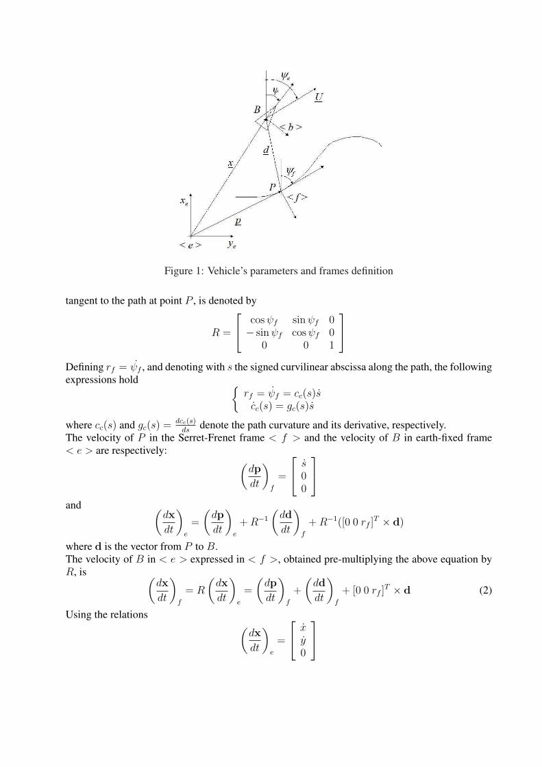
A graphical representation of the nomenclature of the USV kinematics is given in Figure 1, where
variables describing the path-following problem are pointed out too.
2.2 Path-following kinematics
Given the path to be followed by the vehicle, a Serret-Frenet frame < f > that moves along the
path is defined. Such frame is usually called virtual target vehicle and it should be tracked by the
real vehicle. With reference to Figure 1, P is an arbitrary point on the path, < f > is the Serret-
Frenet frame associated to that point and p = [xP yP ]T is the position vector of the point P with
reference to the earth fixed frame < e >. The point B, attached to the vehicle body, can either be
expressed as x = [x y 0]T in < e > or as [s1 y1 0]T in < f >.
The rotation matrix from < e > to < f >, parameterized locally by the angle ψf , which is the
Figure 1: Vehicle’s parameters and frames definition
tangent to the path at point P , is denoted by
R =
cos ψf sin ψf 0− sin ψf cos ψf 0
0 0 1
Defining rf = ψf , and denoting with s the signed curvilinear abscissa along the path, the following
expressions hold{
rf = ψf = cc(s)scc(s) = gc(s)s
where cc(s) and gc(s) = dcc(s)ds
denote the path curvature and its derivative, respectively.
The velocity of P in the Serret-Frenet frame < f > and the velocity of B in earth-fixed frame
< e > are respectively:(
dp
dt
)
f
=
s00
and(
dx
dt
)
e
=
(
dp
dt
)
e
+ R−1
(
dd
dt
)
f
+ R−1([0 0 rf ]T × d)
where d is the vector from P to B.
The velocity of B in < e > expressed in < f >, obtained pre-multiplying the above equation by
R, is(
dx
dt
)
f
= R
(
dx
dt
)
e
=
(
dp
dt
)
f
+
(
dd
dt
)
f
+ [0 0 rf ]T × d (2)
Using the relations(
dx
dt
)
e
=
xy0
(
dd
dt
)
f
=
s1
y1
0
and
[0 0 rf ]T × d =
00
cc(s)s
×
s1
y1
0
=
−cc(s)sy1
cc(s)ss1
0
equation (2) can be rewritten as
R
xy0
=
s(1 − cc(s)y1) + s1
y1 + cc(s)ss1
0
Solving for s1 and y1 yields
s1 =[
cos ψf sin ψf
]
[
xy
]
− s (1 − ccy1)
y1 =[
− sin ψf cos ψf
]
[
xy
]
− ccss1
(3)
Finally, replacing the top two equations of (2) in (3) and introducing the variable β = ψe − ψf
gives the ’kinematic’ model of the vehicle in (s, y) coordinates as
s1 = −s (1 − ccy1) + U cos βy1 = −ccss1 + U sin β
β = re − ccs
where re = ψe = rη(t).
2.3 Dynamics
As mentioned in section 1, the work presented in this paper focuses on the design of a path-
following guidance law at kinematic level, while the generated reference yaw rate is tracked by a
low-level dedicated controller already present on the testbed USV. In particular, the Charlie USV
is equipped with model-based linear and angular velocity controllers, as well as motion estimators.
Thus, a brief discussion of the adopted model of the vehicle dynamics is reported in the following.
For a detailed discussion of the assumptions and experimental results, which led to the definition
of a practical model1 for the Charlie USV dynamics, the reader can refer to (Caccia et al., 2008b).
In particular, since the vessel speed with respect to the water is about proportional to the propeller
revolution rate, experiments carried out with the Charlie USV revealed the impossibility to observe
both these quantities, as well as sway dynamics, using measurements only from onboard GPS and
compass. Thus, sway speed can be neglected and the dynamics can be reduced to:
muur = kuur + ku2ru2
r + kn2δ2n2δ2 + n2 (4)
Irr = krr + kr|r|r|r| + kn2n2 + n2δ (5)
1practical stands for consistent, from the point of view of degree of accuracy, quality in terms of noise and sampling rate of themeasurements
where n is the propeller revolution rate, δ is the rudder angle, mu and Ir are the normalised inertia
terms, ku, ku2r, kr and kr|r| are the drag coefficients, kn2δ2 represents the resistance due to the rudder
and k2n takes into account the vessel longitudinal asymmetries.
Since, as discussed above, in equation (5), the steering torque n2δ has been identified as function
of the propeller revolution rate instead of the advance speed, the rudder action is neglected when
the vehicle is still moving while n is zero. Thus, it is worth noting that the field of validity of the
proposed model of vehicle dynamics is for n > n > 0. As remarked in section 3.3, this forces a
minimum USV speed for guaranteeing manoeuvring capabilities.
3 Guidance and control
3.1 Navigation, guidance and control architecture
A dual-loop hierarchical guidance and control architecture decoupling kinematics and dynamics
is adopted. In the proposed control scheme, the external guidance loop performs position control
generating suitable velocity references according to the desired task, i.e. path-following in this
case. The dynamic controllers have to ensure that the actual rotational and linear speed of the ve-
hicle track the references with sufficient precision to guarantee the overall stability of the system.
Although a rigorous demonstration of system stability is not given, the design of guidance task
functions at the kinematic level is usually very simple as well as the tuning of the kinematic and
dynamic controller parameters on the basis of empirical considerations as discussed in (Caccia,
2007) and (Caccia et al., 2008a).
Figure 2: Dual-loop navigation, guidance and control architecture
As shown in Figure 2, this architecture implements different motion task functions keeping un-
changed the vehicle control and navigation system. In the case of the Charlie USV, a navigation
system relying on model based extended Kalman filters estimates the vessel position x, orienta-
tion and speed x, as well sea current velocity xC , in the earth-fixed frame < e > and surge uand yaw rate r in the body-fixed frame < b >. PI-type linear and angular velocity controllers
are designed following a gain scheduling approach in order to guarantee a specific behaviour, in
terms of closed-loop characteristic equations. A detailed discussion of the Charlie USV navigation
and control system can be found in (Caccia et al., 2008a). Here, it is sufficient to point out that
the kinematic path-following guidance law, computed as discussed in section 3.2, feeds a lower
level PI-type yaw-rate dynamic controller. Although the proof of stability of the overall dual-loop
control scheme is not considered in this paper, the kinematic controller parameters are assumed
to be set such that the rate of change of r∗ is slow enough to be perfectly tracked by the dynamic
controller.
3.2 Kinematic controller design
Usually, the solution to the path-following problem is based on the zeroing of the distances between
the vehicle and a point P on the path, and the angle β between the vehicle’s total velocity vector Uand the tangent to the path at P . With respect to classical approaches in which P is the closest point
on the path, the key idea proposed in this paper is to consider the target point, with its associated
Serret-Frenet frame < f >, moving along the path according to a defined control law, obtaining in
this way an extra controller design parameter.
As discussed in (Lapierre and Soetanto, 2006), the demonstration of stability of the proposed
controller is essentially based on the application of the Barbalat’s lemma and LaSalle’s theorem.
Since the application of LaSalles theorem is restricted to autonomous systems, in the examined
case the fact that the desired forward velocity is a constant allows the system to be considered as
autonomous. In the following, a trace of the main steps in designing the Lyapunov based controller
is given. For a rigorous proof the reader can refer to (Lapierre and Soetanto, 2006).
At first a desired approach angle ϕ is defined as a function of the distance of the USV from the
tangent line to the path in the point P , i.e. y1 in the Serret-Frenet frame < f >. The function ϕ(y1)has to satisfy the constraints ‖ϕ(y1)‖ < π/2, y1ϕ(y1) ≤ 0 and ϕ(0) = 0, stating that the vehicle
heads for the desired path and remains over it once reached.
For instance, the following hyperbolic tangent shaped function, parameterized by kϕ > 0 and
0 < ψa < π/2, with its saturation properties satisfies the above mentioned requirements:
ϕ(y1) = −ψa tanh(kϕy1) (6)
Then, the vehicle approach angle β is imposed to track the desired one ϕ by considering the
candidate Lyapunov function
V =1
2(β − ϕ)2
Its time derivative
V = (β − ϕ)(β − ϕ) = (rη(t) − ccs − ϕ) (β − ϕ)
is negative-semidefinite, V = −k1(β − ϕ)2, when choosing the control law
r∗ =1
η(t)[ϕ − k1(β − ϕ) + cc(s)s] (7)
where k1 ≥ 0.
Since V is lower bounded and V is uniformly continuous, Barbalat’s lemma leads to the conclusion
that limt→+∞ V = 0.
Moreover, the proposed control law makes variables β, s1 and y1 bounded and approaching to the
set E, defined by V =0. The motion of the feedback control system, restricted to E can be studied
considering the Lyapunov function
VE =1
2(s2
1 + y21)
Computing its time derivative
VE = (Ucosβ − s) s1 + Uy1sinβ
it is worth noting that the speed s of the target Serret-Frenet < f > constitutes an additional degree
of freedom that can be controlled in order to guarantee the convergence of the vehicle at the desired
path. In particular, considering that, in the set E, β = ϕ(y1) and that y1sinϕ(y1) ≤ 0 for the choice
of ϕ(y1), the control law
s∗ = U cos β + k2s1 (8)
with k2 > 0 guarantees VE ≤ 0. Since VE is bounded, for Barbalat’s Lemma limt→+∞ VE = 0,
which in turn implies that all trajectories in E satisfy limt→+∞ s1 = 0 and limt→+∞ y1 = 0. Thus
the asymptotically convergence to zero of the variables β, s1 and y1 is guaranteed.
The controller exposed in equation (7) with the virtual target equation of motion (8) has been
implemented on the Charlie USV’s architecture. Experimental results are reported in section 5.
The advantage of the proposed controller are summarised as it follows.
• The nonlinear approach angle ϕ, see equation (6), originally introduced by C. Samson
(Micaelli and Samson, 1993) allows for driving the incidence angle of the robot with respect
to path. Indeed when y1 is high, the desired incidence is ±ψa, i.e. ±π2, that is the vehicle’s
orientation is driven perpendicularly to the path tangent. As y1 reduces, the incidence also
reduces, and vanishes to zero as y1 is zero, i.e. when the vehicle is on the path.
• The virtual target principle, denoted as s, introduces an extra (and virtual) degree of free-
dom to the system. Controlling the virtual target as expressed in equation (8) removes the
classic singularity of the path-following problem exposed in (Micaelli and Samson, 1993).
Indeed, the consideration of the closest point on the path as the target to be tracked by the
vehicle imposes a severe limitation in the domain of attraction of the control. The virtual
target allows for enlarging this domain of attraction to the whole space, thus removing
singularity.
3.2.1 Implementation issues
• Sea current compensation
As discussed in (Caccia et al., 2008a), where the case of straight line following has been
addressed, lateral sea currents are naturally compensated by guidance laws generating a
reference yaw rate as a function only of the range from the target path and its first deriva-
tive. Indeed, thanks to an integrator embedded in the kinematics of the linearized physical
system around the equilibrium point, the vehicle naturally heads in such a way of following
the desired line while compensating lateral sea current. This property, which guarantees lo-
cal stability, is not valid when the reference yaw rate is somehow computed as a function
of a desired heading angle. In this case, the presence of neglected constant sea current
disturbances yields to a steady state error in the range from the desired path.
Since the measurement of sea current is not always available onboard small USVs, and its
estimate can be very imprecise or noisy, operating conditions can require the adoption of
guidance laws neglecting this class of disturbances. How neglecting sea current affects the
proposed path-following guidance law is discussed in the following.
In the equation (7) the term η(t) =[
u2r
U2 + ur
U2 (xc cos ψ + yc sin ψ)]
can be unknown, or
roughly estimated. Anyway, adding some practical constraints the multiplicative noise
term could be neglected. Indeed, considering the typical operative conditions in which the
vehicle surge with respect to the water is higher than the sea current√
x2C + y2
C < ur
the noise function η(t) is always positive and never reaches the zero value.
So, assuming η(t) = 1, i.e. neglecting sea currents, and rewriting the guidance law for r as
r∗ = ϕ − k1(β − ϕ) + cc(s)s
the derivation of V yields:
V = −k1η(t)(β − ϕ)2 + (η − 1)(ϕ + ccs)(β − ϕ)
that is negative outside of the interval limited by zero andη(t)−1k1η(t)
(ϕ + ccs), that defines a
tube around the path that the system is guaranteed to reach.
• Behaviour at path beginning and end
The desired path has typically a beginning and an end, i.e. is typically defined for con-
strained values of the curvilinear abscissa. Thus, the evolution of s according to (8) has to
be constrained in the interval s ∈ [0 sMAX ]. In particular, forcing s to 0 or sMAX when its
evolution would lead it outside of the desired interval is equivalent to force the vehicle to
follow the tangent to the path in its beginning or end point respectively. From a practical
point of view, this is usually not dangerous when the vehicle approaches the path starting
point along its tangent. On the other hand, a vehicle which tries to move along the path
tangent after its end can be very dangerous. So, safety manoeuvres, e.g. rotating at constant
yaw rate, have to be executed when the vehicle reaches the end of the path, i.e. s∗ = sMAX .
• Generic path software representation
The issue of generic representation of paths in the software implementation has been ad-
dressed too. Although only explicit representations through mathematical functions can
guarantee exact computation of the path properties for every value of the curvilinear ab-
scissa s, from the point of view of software implementation such an approach would limit
the possible paths to a set of classes of functions known by the system. Thus, a generic
path is represented as a sequence of points, discretised for s = s0 , . . . , sN = sMAX ,
with the corresponding tangent vector and curvature. For intermediate values of s, the path
parameters are linearly interpolated: p(s) = p(si) +p(si+1)−p(si)
si+1−si(s− si) for s ∈ (si , si+1)
where p can represent the path point coordinates, tangent vector components or curvature.
3.3 Heuristic speed adaptation
The above discussed guidance law drives an ideal vessel with no leeway with respect to the water
over a desired path. Indeed, the actual testbed USV is characterized by physical limitations on the
maximum yaw rate and unmodeled sway with respect to the water. The result is that the vehicle,
when working at constant surge, can execute large U-turns for heading the path or sliding away
from the path when executing sharp curves.
The proposed solution to this issue arises from human common behavior when driving a vehicle:
while approaching a curve or when tricky manoeuvres are needed, advance speed is reduced with
respect to the desired one u∗ established by the human operator or mission controller.
Assuming that the vehicle speed is within a minimum Umin, needed to allow manoeuvring capa-
bilities (see section 2.3 for details), and a maximum Umax, a heuristic law has been introduced in
the global regulation schema to improve the guidance and control system performances.
From this concept arises the equations that model such a behavior; first, an adaption for the maxi-
mum surge speed is computed in function of the actual yaw rate requested by the controller:
u∗1MAX
=Umax − Umin
2+
Umax − Umin
2
[
cos
(
πr∗
rsat
)]
(9)
where Umax, Umin and rsat are parameters of the adaptation law. This reduces surge speed when
the vehicle orientation is far from the required heading in order to speed up the convergence to
the desired approach angle. Thus, a second adapted maximum reference surge speed is computed
on the basis of a prediction of the maximum curvature of the path inside a predefined prediction
horizon:
u∗2MAX
= Umin + (Umax − Umin)[
1 − tanh2 (kucmax)]
(10)
where ku is a free parameter and cmax is the maximum value of cc(s), with s in [s; s + h], h is the
prediction horizon. This helps the vehicle to maintain its position above high curvature segments
of the path. Finally, the adapted maximum reference surge speed is computed as the minimum
between u∗1MAX
and u∗2MAX
:
u∗MAX = min
(
u∗1MAX
, u∗2MAX
)
and the adapted reference surge is
u∗ = min (u∗, u∗MAX)
The reader should note that the expression (9) contains the control input r∗, thus introducing a
coupling between the yaw and surge control inputs. The authors are aware of the algebraic loop
introduced by this method. Nevertheless, note that this coupling will induce a reduced surge ve-
locity. The improvement of this method is clearly exposed in section 5, where experimental results
validated the proposed approach.
4 Charlie USV
The Charlie USV (see Figure 3) is a small catamaran-like shaped prototype vehicle, originally
developed and exploited, during the XIX Italian expedition to Antarctica in 2003-’04, by the CNR-
ISSIA for the sampling of the sea surface microlayer and immediate subsurface for the study of
the sea-air interaction (Caccia et al., 2005). Charlie is 2.40 m long, 1.70 m wide and weighs
about 300 Kg in air. The propulsion system of the vehicle is composed by a couple of DC motors
(300 W @ 48 V), with a set of servo-amplifiers which provide a proportional-integral-differential
(PID) control of the propeller revolution rates. In the current release, the vehicle is equipped
with a rudder-based steering system, where two rigidly connected rudders, positioned behind the
thrusters, are actuated by a brushless DC motor. The navigation instrumentation set is constituted
by a GPS Ashtech GG24C integrated with a KVH Azimuth Gyrotrac able to compute the True
North. Electrical power supply is provided by four 12 V @ 40 Ah lead batteries integrated with
four 32 W triple junction flexible solar panels. The on-board real-time control system, developed
in C++, is based on GNU/Linux and run on a Single Board Computer (SBC), which supports
serial and Ethernet communications and PC-104 modules for digital and analog I/O (Bruzzone
et al., 2008). An overview of the Charlie project, including a detailed description of the vehicle
and a summary of its applications, can be found in (Caccia et al., 2007). Nominal values for
Figure 3: The Charlie USV
the parameters of the Charlie USV dynamics, as modelled in equations 4 and 5, can be found in
(Caccia et al., 2008b).
5 Experimental results
Experimental tests have been carried out in the Genova Pra harbor (see Figure 4, a calm water
channel devoted to rowing races; the site is usually beaten by a 20-30 knots wind. Results obtained
during a preliminary session of trials, carried out in December 2006, are reported and discussed in
(Bibuli et al., 2007), where the integration with backstepping techniques for handling the vehicle
dynamics has been considered too. The tests discussed in the following have been performed on
December 22nd 2008 in no wind conditions and on March xxth 2009 in bla bla conditions. Field
Figure 4: Genova Pra test site (Google Earth view)
trials had two basic goals: i) proving the practical validity of the proposed theoretical guidance laws
(7) and (8); ii) evaluating the benfits given by heuristic speed adaptation. A set of metrics have
been defined for measuring the main performance criterium, i.e. the capability of the vehicle of
following the desired path: the area between the actual and the reference path measures the integral
performance along the path, the bla bla. In this context, the kinematic guidance algorithm, with
different approach angles, has been tested without speed adaptation and with the guidance law
integrated with the speed adaptation heuristic, accomplishing dynamic control with the Charlie
USV standard PI gain-scheduling yaw-rate controller. The vehicle navigation system consisted of
conventional extended and linear time-varying Kalman filters processing GPS and compass mea-
surements. Experimental identification of the vehicle dynamics allowed the open-loop estimate of
its surge speed with respect to the water, on the basis of the normalised propeller revolution rate
and rudder deflection by online integrating equation (4). This operation is equivalent to implement
a kind of virtual velocity sensor consisting of an open-loop model-based predictor in the manner
presented in (Caccia and Veruggio, 1999). For a detailed discussion of the Charlie USV navigation
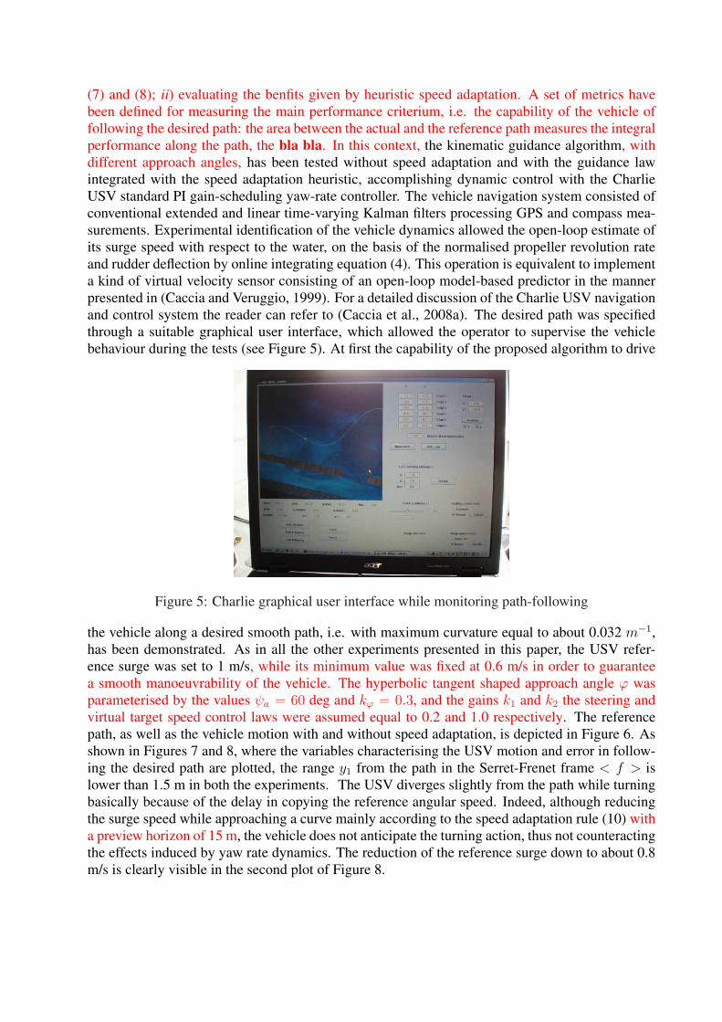
and control system the reader can refer to (Caccia et al., 2008a). The desired path was specified
through a suitable graphical user interface, which allowed the operator to supervise the vehicle
behaviour during the tests (see Figure 5). At first the capability of the proposed algorithm to drive
Figure 5: Charlie graphical user interface while monitoring path-following
the vehicle along a desired smooth path, i.e. with maximum curvature equal to about 0.032 m−1,
has been demonstrated. As in all the other experiments presented in this paper, the USV refer-
ence surge was set to 1 m/s, while its minimum value was fixed at 0.6 m/s in order to guarantee
a smooth manoeuvrability of the vehicle. The hyperbolic tangent shaped approach angle ϕ was
parameterised by the values ψa = 60 deg and kϕ = 0.3, and the gains k1 and k2 the steering and
virtual target speed control laws were assumed equal to 0.2 and 1.0 respectively. The reference
path, as well as the vehicle motion with and without speed adaptation, is depicted in Figure 6. As
shown in Figures 7 and 8, where the variables characterising the USV motion and error in follow-
ing the desired path are plotted, the range y1 from the path in the Serret-Frenet frame < f > is
lower than 1.5 m in both the experiments. The USV diverges slightly from the path while turning
basically because of the delay in copying the reference angular speed. Indeed, although reducing
the surge speed while approaching a curve mainly according to the speed adaptation rule (10) with
a preview horizon of 15 m, the vehicle does not anticipate the turning action, thus not counteracting
the effects induced by yaw rate dynamics. The reduction of the reference surge down to about 0.8
m/s is clearly visible in the second plot of Figure 8.
−300 −280 −260 −240 −220 −200 −180 −160
−80
−60
−40
−20
0
20
Charlie USV Path−Following 22/12/2008: smooth path, max(c)=0.032 m−1
x [m
]
y [m]
reference pathpath without speed adaptationpath with speed adaptation
Figure 6: Path-Following: smooth path. Charlie USV estimated and desired path.
On the other hand, the model-based tuning of the yaw rate controller (Caccia et al., 2008a) allows
a quite smooth action of the rudder actuator minimising the mechanical stress of the system.
The benefits given by speed adaptation while following high curvature paths and inverting the
motion direction are pointed out by the second set of manoeuvres where the USV is requested to
follow curves of similar shape of the previous one, but with a maximum curvature of 0.063 m−1.
The two paths were shifted in the x-y plane due to the traffic conditions inside the regatta field
where trials were performed. In this case, as clearly visible in Figure 9, the reduction of speed
while approaching a curve, given by the speed adaptation rule (10), keeps the vehicle closer to the
desired path moving along high curvature bents. Moreover, when reducing its surge while turning
according to the speed adaptation rule (9), the vehicle executes U-turns in a smaller area recovering
the desired path without remarkable overshoots induced by the combination of its constrained yaw
rate and high reference surge speed.
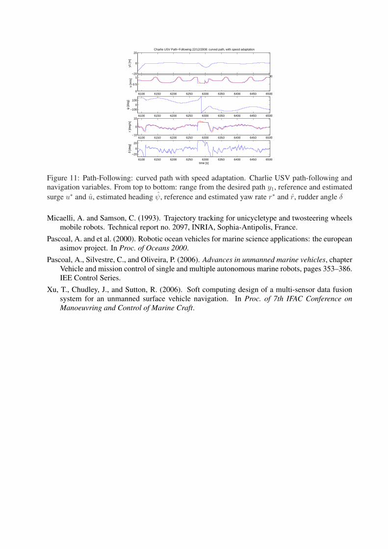
Figures 10 and 11, where the guidance and navigation variables of the USV are plotted, pro-
vide some quantitative measurements of the benefits obtained by heuristically adapting the vehicle
speed. The adaptation of the surge speed down to 0.6 m/s reduces the range y1 from the path in the
Serret-Frenet frame < f > to about 1.2 m with respect to more than 2 m when no speed adaptation
rule is applied. In addition, the overshoot when re-tracking the desired path in the opposite direc-
tion decreases from more than 7 m to about 1 m, while the approximate diameter of the U-turn
decreases from about 20 m to less than 8 m. It is worth noting that the apparent higher use of
the rudder when speed adaptation is applied is due by the fact that, according to the USV yaw
dynamics (5), at lower surge, i.e. at lower propeller revolution rate n, higher rudder angles are
required for obtaining the same yaw rate.
The benefits given by adapting the surge speed in function of the actual yaw rate requested by the
controller are pointed out when the Charlie USV followed a straight line in alternate directions as
shown in Figures 12 and 13. In particular, the reduction of the USV surge speed with its yaw rate
according to equation (9) dramatically restricts the circle-like path drawn by the vehicle while ex-
ecuting a U-turn. Indeed, with a default reference surge of 1 m/s, Charlie followed a path of about
22.5 m of diameter when no speed adaptation was applied, which reduced to about 10 m in the
case of heuristic adaptation of the reference surge. The overshoot and oscillations, once reached
4560 4580 4600 4620 4640 4660 4680 4700−5
0
5Charlie USV Path−Following 22/12/2008: smooth path, no speed adaptation
y1 [m
]
4560 4580 4600 4620 4640 4660 4680 47000
0.5
1
u [m
/s]
4560 4580 4600 4620 4640 4660 4680 4700
−100
0
100
ψ [d
eg]
4560 4580 4600 4620 4640 4660 4680 4700−10
0
10
r [d
eg/s
]
4560 4580 4600 4620 4640 4660 4680 4700
−20
0
20
δ [d
eg]
time [s]
Figure 7: Path-Following: smooth path without speed adaptation. Charlie USV path-following and
navigation variables. From top to bottom: range from the desired path y1, reference and estimated
surge u∗ and u, estimated heading ψ, reference and estimated yaw rate r∗ and r, rudder angle δ
the target path, reduced in a similar way. Moreover, the proposed guidance law demonstrated its
capability in managing inversions of direction in following a line without any singularity.
6 Conclusions
In this paper the problem of path-following in two-dimensional space for under-actuated unmanned
surface vehicles has been handled through the definition of a nonlinear Lyapunov-based guidance
law, yielding convergence of the path following error coordinates to zero. Singularities of the algo-
rithm are removed thanks to the introduction of the target dynamic. The proposed solution, which
generates reference surge and yaw rate, has been integrated with the control system of an exist-
ing USV managing its dynamics in a conventional nested-loop architecture. Although a rigorous
demonstration of system stability is not given, the design of the path-following guidance task at
the kinematic level has been validated in extended field trials carried out with the Charlie USV,
developed by CNR-ISSIA and employed as a testbed for the evaluation of numerous guidance and
control techniques (Caccia et al., 2007).
Moreover, experimental results confirmed the expected improvements of the tracking response
of the proposed technique obtained with the integration of the guidance law with some heuristic
approaches, facing the problem of speed of advance adaptation based on path curvature measure-
ment and steering action prediction. Although these heuristic approaches introduce an algebraic
loop through a coupling between the yaw and surge control inputs, dramatic benefits in terms of
tracking precision and execution of human-like manoeuvres have been verified experimentally.
Although experimental results show a manoeuvering precision of the order of a few tenths of
centimeters, which is generically satisfactory for underactuated marine systems, a metric-based
comparison with other guidance laws for path-following proposed in the literature would allow a
quantitative evaluation of system performances. The implementation and integration in the vehicle
control system of a set of path-following controllers, as well as the execution of comparative trials
for straight line and generic path following, is part of the Charlie USV basic research plan.
4980 5000 5020 5040 5060 5080 5100 5120−5
0
5Charlie USV Path−Following 22/12/2008: curved path, with speed adaptation
y1 [m
]
4980 5000 5020 5040 5060 5080 5100 51200
0.5
1
u [m
/s]
4980 5000 5020 5040 5060 5080 5100 5120
−100
0
100
ψ [d
eg]
4980 5000 5020 5040 5060 5080 5100 5120−10
0
10
r [d
eg/s
]
4980 5000 5020 5040 5060 5080 5100 5120
−20
0
20
δ [d
eg]
time [s]
Figure 8: Path-Following: smooth path with speed adaptation. Charlie USV path-following and
navigation variables. From top to bottom: range from the desired path y1, reference and estimated
surge u∗ and u, estimated heading ψ, reference and estimated yaw rate r∗ and r, rudder angle δ
Moreover, future works head towards the mathematical formalization of the heuristic laws and the
demonstration of stability of the nested loop guidance and control system.
7 Acknowledgments
This work has been funded by the common research project ”Sensor-based guidance and control of
autonomous marine vehicles: path-following and obstacle avoidance” between CNR-ISSIA Gen-
ova, Italy, and CNRS-LIRMM Montpellier, France, for the years 2006-2007, and by PRAI-FESR
within the project: ”Coastal and harbor underwater anti-intrusion system” for the years 2005-2007.
The authors wish to thank Giorgio Bruzzone and Edoardo Spirandelli for their fundamental sup-
port in developing, maintaining and operating the Charlie USV. Special thanks to the members of
A.D.P.S. Pra Sapello for their kind support to sea trials.