PATHS, TREES, AND THE COMPUTATIONAL STRENGTH
OF SOME RAMSEY-TYPE THEOREMS
A Dissertation
Submitted to the Graduate School
of the University of Notre Dame
in Partial Fulfillment of the Requirements
for the Degree of
Doctor of Philosophy
by
Stephen Flood
Peter Cholak, Director
Graduate Program in Mathematics
Notre Dame, Indiana
May 2012
PATHS, TREES, AND THE COMPUTATIONAL STRENGTH
OF SOME RAMSEY-TYPE THEOREMS
Abstract
by
Stephen Flood
An industry has arisen dedicated to the study of the interplay between com-
binatorial principles and computational strength. In particular, much work has
been done on theorems similar to Ramsey’s Theorem and to Weak Konig’s Lemma.
We study two related principles, which are interesting both for their combinatorial
form and for their computational content.
We begin by studying the computational strength of a version of Ramsey’s
Theorem that combines features of finite and infinite Ramsey theory. Paul Erdos
and Fred Galvin proved that for each coloring f , there is an infinite set that is
“packed together” which is given “a small number” of colors by f . We show
that this theorem is close in computational strength to standard Ramsey’s Theo-
rem, giving arithmetical bounds for solutions to computable instances. In reverse
mathematics, we show that that this Packed Ramsey’s Theorem is equivalent to
Ramsey’s Theorem for exponents n 6= 2. When n = 2, we show that it implies
Ramsey’s Theorem, and that it does not imply ACA0.
We next introduce a new combinatorial principle, called RKL, which combines
features of Weak Konig’s Lemma and Ramsey’s Theorem. We show that this
principle is strictly weaker than both WKL0 and RT22, and that it is strictly stronger
Stephen Flood
than RCA0. We also consider two generalizations of this principle. We obtain the
surprising result that these stronger principles are closer in strength to RT22 than
they are to WKL0.
CONTENTS
FIGURES . . . . . . . . . . . . . . . . . . . . . . . . . . . . . . . . . . . . iv
ACKNOWLEDGMENTS . . . . . . . . . . . . . . . . . . . . . . . . . . . v
CHAPTER 1: INTRODUCTION AND BACKGROUND . . . . . . . . . . 11.1 Introduction . . . . . . . . . . . . . . . . . . . . . . . . . . . . . . 11.2 Reverse mathematics . . . . . . . . . . . . . . . . . . . . . . . . . 2
1.2.1 Second order arithmetic . . . . . . . . . . . . . . . . . . . 21.2.2 The base system RCA0 . . . . . . . . . . . . . . . . . . . . 41.2.3 Proofs over RCA0 . . . . . . . . . . . . . . . . . . . . . . . 61.2.4 Subsystems of second order arithmetic . . . . . . . . . . . 71.2.5 First-order subsystems of second order arithmetic . . . . . 9
1.3 Computability theory . . . . . . . . . . . . . . . . . . . . . . . . . 101.3.1 Computability theory and trees . . . . . . . . . . . . . . . 101.3.2 Computability theory and Ramsey’s Theorem . . . . . . . 13
CHAPTER 2: A PACKED RAMSEY’S THEOREM AND COMPUTABIL-ITY THEORY . . . . . . . . . . . . . . . . . . . . . . . . . . . . . . . 172.1 Introduction . . . . . . . . . . . . . . . . . . . . . . . . . . . . . . 17
2.1.1 Summary of results . . . . . . . . . . . . . . . . . . . . . . 212.1.2 Outline . . . . . . . . . . . . . . . . . . . . . . . . . . . . 222.1.3 A proof of PRT1
k . . . . . . . . . . . . . . . . . . . . . . . 232.2 A tree proof of PRT2
k . . . . . . . . . . . . . . . . . . . . . . . . . 252.2.1 Outline . . . . . . . . . . . . . . . . . . . . . . . . . . . . 262.2.2 Largeness for exponent 2 . . . . . . . . . . . . . . . . . . . 262.2.3 The construction . . . . . . . . . . . . . . . . . . . . . . . 28
2.3 A low2 proof of PRT2k . . . . . . . . . . . . . . . . . . . . . . . . . 31
2.3.1 The strategy . . . . . . . . . . . . . . . . . . . . . . . . . . 322.3.2 Conditions . . . . . . . . . . . . . . . . . . . . . . . . . . . 332.3.2.1 Pre-conditions . . . . . . . . . . . . . . . . . . . . . . . 342.3.2.2 The tree . . . . . . . . . . . . . . . . . . . . . . . . . . . 35
ii
2.3.3 The module for even stages . . . . . . . . . . . . . . . . . 352.3.3.1 Forcing divergence . . . . . . . . . . . . . . . . . . . . . 362.3.3.2 Forcing convergence . . . . . . . . . . . . . . . . . . . . 362.3.4 The module for odd stages . . . . . . . . . . . . . . . . . . 372.3.5 Putting it all together . . . . . . . . . . . . . . . . . . . . 38
2.4 Tools for proving PRTnk . . . . . . . . . . . . . . . . . . . . . . . . 392.4.1 Trees and colorings of n-tuples . . . . . . . . . . . . . . . . 392.4.2 Largeness for exponent n . . . . . . . . . . . . . . . . . . . 402.4.2.1 Motivation . . . . . . . . . . . . . . . . . . . . . . . . . 402.4.2.2 Definitions and lemmas . . . . . . . . . . . . . . . . . . 40
2.5 A tree proof of PRTnk . . . . . . . . . . . . . . . . . . . . . . . . . 442.5.1 The strategy . . . . . . . . . . . . . . . . . . . . . . . . . . 452.5.2 Obtaining the helper colorings . . . . . . . . . . . . . . . . 472.5.3 Selecting a sequence of blocks . . . . . . . . . . . . . . . . 512.5.4 Putting it all together . . . . . . . . . . . . . . . . . . . . 52
2.6 Lower bounds and reversals . . . . . . . . . . . . . . . . . . . . . 532.6.1 Sharpness of number of colors . . . . . . . . . . . . . . . . 532.6.2 Using PRTn to prove RTn over RCA0 . . . . . . . . . . . . 552.6.3 Σ0
n sets and PRTnk . . . . . . . . . . . . . . . . . . . . . . . 57
CHAPTER 3: REVERSE MATHEMATICS AND A RAMSEY-TYPE KONIG’SLEMMA . . . . . . . . . . . . . . . . . . . . . . . . . . . . . . . . . . . 583.1 Introduction . . . . . . . . . . . . . . . . . . . . . . . . . . . . . . 58
3.1.1 Working in second order arithmetic . . . . . . . . . . . . . 593.2 Reverse mathematics of RKL . . . . . . . . . . . . . . . . . . . . . 603.3 Trees generated by sets of strings . . . . . . . . . . . . . . . . . . 633.4 Arithmetically-definable trees . . . . . . . . . . . . . . . . . . . . 67
3.4.1 Subsets, co-subsets, and trees . . . . . . . . . . . . . . . . 68
BIBLIOGRAPHY . . . . . . . . . . . . . . . . . . . . . . . . . . . . . . . 72
iii
FIGURES
1.1 The big 5 subsystems and RT22. . . . . . . . . . . . . . . . . . . . 16
2.1 A is packed for φ. . . . . . . . . . . . . . . . . . . . . . . . . . . . 19
3.1 The reverse mathematical strength of RKL. . . . . . . . . . . . . . 70
3.2 The reverse mathematical strength of RKL and PRT. . . . . . . . 71
iv
ACKNOWLEDGMENTS
First and foremost, I would like to thank my advisor Peter Cholak for his
patience, guidance, and constant exhortations to prove theorems.
I would like to give special thanks to Francis Su, Kevin O’Neill, and Rosalie
Carlson. Their enthusiasm and creativity has been an inspiration.
I also thank the many logicians who have aided and encouraged this work.
Above all, Damir Dzhafarov has helped focus my questions and given many useful
suggestions. His feedback on my papers has greatly improved them. Wei Wang
also gave helpful feedback and some very useful suggestions at an early stage of
my work on PRT2k. Keita Yokoyama generously allowed me to include his proof
of Theorem 3.3.9 in my paper on RKL. And throughout the past five years,
my office-mates Christopher Porter, Joshua Cole, Sean Walsh, Logan Axon, and
Quinn Culver have consistently expressed their interest and encouragement.
I thank the University of Notre Dame for their many efforts to build a campus
and academic community that embraces the whole person. I also thank the NSF
for providing partial support for this research through EMSW21-RTG 0353748,
0739007, and 0838506.
And finally, I would like to express my deep gratitude to my family, friends,
and church family. They have walked with me through every stage of this journey.
v
CHAPTER 1
INTRODUCTION AND BACKGROUND
1.1 Introduction
We study the interplay between combinatorics and computation. Together,
computability theory and reverse mathematics provide a robust set of tools for
studying the “computational strength” of theorems in infinite combinatorics. Two
of these theorems have particularly interesting computational strength: Ramsey’s
Theorem and Weak Konig’s Lemma.
Weak Konig’s Lemma is the statement “every infinite binary tree has an infinite
path.” Weak Konig’s Lemma is essentially the statement “2N is compact,” and
is equivalent in reverse mathematics to many theorems about compactness (see
[22]). In computability theory, the Low Basis Theorem of [18] says that every
computable infinite binary tree has a low infinite path.
Ramsey’s Theorem is a generalization of the pigeonhole principle. The infinite
form of Ramsey’s Theorem says that for any coloring f of n element subsets of
N with k colors, there is an infinite set which is given a single color by f . The
computational strength of this theorem has been studied extensively, particularly
in [1, 2, 16, 19, 21]. 1
By studying variants of Ramsey’s Theorem and Weak Konig’s Lemma, we can
deepen our understanding of the relationship between specific combinatorial fea-
1The previous two paragraphs appear in [10] in a slightly modified form.
1
tures and computational strength. We begin in Chapter 2 by studying a theorem
of Erdos and Galvin that blends features of finite and infinite Ramsey’s Theorem.
We continue in Chapter 3 by studying a new combinatorial principle that blends
features of Ramsey’s Theorem and Weak Konig’s Lemma.
We will present the motivation, combinatorial background, and a detailed sum-
mary of results at the beginning of each chapter. In the remainder of this chapter,
we will give background on the two notions of “computational strength” that we
study: computability theory and reverse mathematics. In Section 1.2, we discuss
reverse mathematics. Chapter 3 will make frequent use of the material discussed
in Section 1.2.2. In Section 1.3, we discuss two aspects of computability theory.
Section 1.3.1 surveys some results on the computational complexity of trees, which
we will be used during the proofs of Chapter 2. We close in Section 1.3.2 by sur-
veying some major results concerning the strength of infinite Ramsey’s Theorem.
1.2 Reverse mathematics
The standard introduction to, and reference for, reverse mathematics is [22].
Our goal here to highlight the connections between reverse mathematics and com-
putability theory. A key intuition of reverse mathematics is that the statement “T1
implies T2 over RCA0” essentially means that “T2 is proved using T1, computable
constructions, and computable verifications.” We will return to this intuition with
greater detail in Section 1.2.3.
1.2.1 Second order arithmetic
In reverse mathematics, we formalize theorems of different areas of mathemat-
ics using a single language: second-order arithmetic. Because it is arithmetic, we
2
have symbols for 0, 1,+,×, and <. Because it is second order, we can use two
sorts of variables: one for natural numbers and one for sets of natural numbers.
We also use the symbol ∈, and we have equality for number variables.
A model of this language has the form M = (N, S(M), 0, 1,+,×, <). Here N
denotes the first order part of M (the collection of numbers which exist in the
model), and S(M) denotes the second order part (the collection of sets which
exist in the model). A model of second order arithmetic is often abbreviated
M = (N, S(M)).
Note that in reverse mathematics, N refers to the first order part of some
(often unspecified, possibly non-standard) model of arithmetic. We will write ω
to refer to the first order part of the true natural numbers, when it is important
to distinguish between the two.
We also include (in our language) additional symbols for set parameters and
number parameters, and use a natural deduction system as the background logical
axioms. More on natural deduction systems, which are equivalent in strength to
the other standard logical systems, can be found in [24], (particularly Chapters 1
and 2).
When presented with an existential statement, we generally work with an
“arbitrary witness” for this statement. Arbitrary set parameters give a formal
analog of these witnesses in our formal system. When our proof is complete,
this system contains logical rules which eliminate the use of the set parameter by
an appeal to the original existential assumption. Thus, set parameters will not
appear in the theorems studied. Instead, they are used within individual proofs,
and axiom schemes are stated to cover all possible sentences obtained by assigning
different parameters to free variables.
3
We define levels of formula complexity as usual, with the one important remark
that the presence of set parameters does not influence a formula’s complexity.
Definition 1.2.1. A formula is ∆00 = Σ0
0 = Π00 if it has only bounded number
quantifiers, and no set quantifiers. A formula is Σ0n+1 if it has the form (∃x)ψ(x)
for ψ a Π0n formula, and a formula is Π0
n+1 if its negation is Σ0n+1. A formula θ(x)
is ∆0n if there is a Π0
n formula ψ(x) and a Σ0n formula φ(x) such that (∀x)[θ(x)↔
ψ(x)↔ φ(x)]. A formula is arithmetical if it is ∆0n for any n.
A formula is Π11 if it has the form (∀X)ψ(X), where ψ is arithmetical. A
formula is Σ1n if it is the negation of a Π1
n formula. A formula is Π1n+1 if it has the
form (∀X)ψ(X), where ψ is Σ1n. A formula θ(x) is ∆1
n if there is a Π1n formula
ψ(x) and a Σ1n formula φ(x) such that (∀x)[θ(x)↔ ψ(x)↔ φ(x)].
1.2.2 The base system RCA0
In order to compare the strength of theorems in second order arithmetic, we
first require a set of background axioms. Let Γ be a collection of formulas. We
say that T1 implies T2 over Γ, if there is a proof of T2 from Γ ∪ {T1}. We will say
that we work over Γ, or that Γ is our base system, to say that the implications
being discussed hold over Γ. We will work almost exclusively with the base system
RCA0, which roughly corresponds to computable mathematics.
Statement 1.2.2. RCA0 is the axiom scheme that consists of:
1. The ordered semi-ring axioms (the usual rules for 0, 1,+,×, <), denoted Q.
2. ∆01 comprehension, denoted ∆0
1-CA. This asserts that each ∆01 definable
set exists. More formally, ∆01-CA is the axiom scheme which, for each Π0
1
4
formula φ(x,X) and each Σ01 formula ψ(x,X), asserts
(∀X)[(∀x)[ψ(x,X)↔ φ(x,X)] =⇒ (∃Y )(∀x)[x ∈ Y ↔ ψ(x,X)]],
3. Σ01 induction, written IΣ0
1. This is the axiom scheme asserting, for each Σ01
formula φ(x) with free variable x, that
φ(0) ∧ (∀x)[φ(x)→ φ(x+ 1)] −→ (∀x)φ(x)
Inside RCA0, we have access to a number of other first order principles, which
we freely use in our verifications. We will discuss the relationship between these
principles in more generality in Section 1.2.5.
Remark 1.2.3. In RCA0, the following are provable:
1. Π01 induction, written IΠ0
1.
2. Σ01 least-element principle, written LΣ0
1. This is the axiom scheme asserting,
for each Σ01 formula φ(x) with free variable x, that
(∃x)φ(x) −→ (∃x)[φ(x) ∧ (∀y < x)¬φ(y)]
3. Π01 least-element principle, written LΠ0
1.
4. Σ01 bounding, written BΣ0
1. This is the axiom scheme asserting, for each Σ01
formula φ(x, y) with free variables x, y, that
(∀a)[(∀x < a)(∃y)φ(x, y) −→ (∃b)(∀x < a)(∃y < b)φ(x, y)]
5
5. It is possible to iterate an arbitrary function of the second order part an
arbitrary finite number of times. This formal axiom, denoted PREC, states:
(∀m)(∀f a total function)(∃g a total function)
[g(0) = m ∧ (∀z)[g(z + 1) = f(g(z))]].
In fact, as Hirschfeld and Shore show in [12], RCA0 can be stated in an equiv-
alent form by replacing IΣ01 by the combination of PREC and induction for all
sets in S(M). This gives additional support for the suggestion in [22] that RCA0
corresponds roughly to “computable mathematics.”
Remark 1.2.4. It is also important to note that a number of standard first order
proof techniques cannot be proved from RCA0. In particular, BΠ01, BΣ0
2, I∆02, and
L∆02 are all independant of RCA0.
An important intuition is that RCA0 lacks the tools required to perform ver-
ifications which reference functions of high enough arithmetical complexity. For
example, verifications that use ∅′-computable functions often fail in RCA0, or at
least require additional subtlety.
1.2.3 Proofs over RCA0
Given a Π12 axiom T1, we often wish to give a proof of some Π1
2 sentence T2
over RCA0. Working over RCA0 gives us access to three types of steps (beyond
the usual logical rules) that we can use in our proof:
1. Describe how to compute a new set from a given set parameter,
2. Apply T1 to a set parameter X (obtained previously), obtaining a new set
parameter Y (representing a solution of T1 for the instance X), and
6
3. Prove an arithmetical fact using IΣ01 and/or the semi-ring axioms.
Intuitively, (1) and (2) correspond to constructions, because they give us the
ability to begin with one set X and to obtain a new set Y with a certain desired
property. Intuitively, (3) is used in the verification that the constructions behave
as desired (or expected).
To be more precise, note that most Π12 theorems T1 have the form
(∀X)[X has property P =⇒ (∃Y )Q(X, Y )].
Thus to apply T1, and obtain the desired instance Y , we must first verify that X
does indeed have property P . Often, P is an arithmetical statement about X.
Furthermore, if we obtained X using ∆01-CA, we simply know that X is a set.
Because ∆01-CA does not say that X has any specific property, we must verify
statements about X ourselves.
It is important to note that many arithmetical statements cannot be proved us-
ing computable methods alone, and certainly not with Σ01 induction alone. There-
fore, proofs in reverse mathematics must be careful when verifying that X truly
has property P .
1.2.4 Subsystems of second order arithmetic
There are five central systems in reverse mathematics, sometimes called the
“big five.” In order of (strictly) increasing strength, they are: RCA0, WKL0,
ACA0, ATR0, and Π11-CA. Each includes RCA0, together with a more powerful set
comprehension axiom or axiom scheme. The more powerful the comprehension
principle, the more complicated the sets that can be “built” in proofs. In this
thesis, we will only work with the first three of these systems: RCA0, WKL0 and
7
ACA0.
Statement 1.2.5. WKL0 consists of RCA0 together with the statement:
(∀T )(∃P )[T is an infinite binary tree =⇒ P is a path through T ]
Weak Konig’s Lemma is equivalent to many theorems about compactness.
Statement 1.2.6. ACA0 consists of RCA0 together with the statement
(∀X)(∃Y )[x ∈ Y ⇐⇒ φ(x,X)]
for each arithmetical formula φ(x,X).
It is well known that ACA0 is equivalent to the existence of the jump. ACA0 is
often equivalent to theorems asserting the existence of limits.
For any set Z and any arithmetical θ with a single free set and number variable,
we can define the set θZ = {x : θ(x, Z)}. Note that ACA0 essentially says that we
can iterate Z 7→ θZ a fixed, (standard) finite number of times.
Statement 1.2.7. ATR0 consists of RCA0 together with the axiom scheme which,
for each arithmetical formula θ, asserts “for any well ordering X, the set defined
by iterating Z 7→ θZ along X exists.”
ATR0 is the weakest subsystem of arithmetic where it is possible to develop
the basic a theory of ordinal arithmetic [13].
Statement 1.2.8. Π11-CA consists of RCA0 together with statement
(∀X)(∃Y )[x ∈ Y ⇐⇒ φ(x,X)]
8
for each Π11 formula φ(x,X).
For more on these systems, including an overview of the strength of many
different theorems, see [22].
1.2.5 First-order subsystems of second order arithmetic
In this section, we consider the first order principles of induction, least ele-
ment, and bounding discussed in Section 1.2.2, now stated for formulas of various
complexity. To define these principles, simply replace Σ01 with Γ ∈ {Π0
n,Σ0n,∆
0n}
in the both the name and the definition of the Σ01 analog.
We begin by comparing the strength of these first order principles. We write
exp to denote the formula asserting that the exponential function is total. Note
that exp is provable from IΣ01. Working over Q+ IΣ0
0 +exp, these principles form
a linear hierarchy of strength.
Theorem 1.2.9 (Gandy, Kirby, Paris, and Slaman). Over Q+ IΣ00 +exp,
1. IΣ0n ↔ IΠ0
n ↔ LΣ0n ↔ LΠ0
n,
2. BΠ0n ↔ BΣ0
n+1 ↔ I∆0n+1 ↔ L∆0
n+1,
3. IΣ0n+1 =⇒ BΣ0
n+1 =⇒ IΣ0n.
While interesting in their own right, induction principles are not immediately
informative from the perspective of “computable mathematics.” Hirschfeldt and
Shore introduced the principle PRECn, which roughly states that every Π0n−1-
definable function can be iterated an arbitrary finite number of times. For each
n, Hirschfeldt and Shore show that PRECn is equivalent to IΣ0n over a relatively
weak induction scheme.
9
Definition 1.2.10 (Hirschfeldt and Shore [12]). PRECn is the axiom scheme
which asserts for each Π0n−1 formula φ(x, y): if φ defines a total function, then
(∀z)(∀m)(∃σ)[|σ| = z ∧ σ(0) = m ∧ (∀i < z)[φ(σ(i), σ(i+ 1))]]
Proposition 1.2.11 (Hirschfeldt and Shore [12]). For each n ∈ ω,
PRECn is equivalent to IΣ0n over Q+ ∆0
1-CA + I∆01.
1.3 Computability theory
For an introduction to computability theory, see of Part A of [23]. Our goal
here is to provide background, and to introduce some results which will be used
in Chapter 2.
1.3.1 Computability theory and trees
In Chapter 2 we will frequently define functions via initial segments. We will
use trees to organize these definitions, leading us to identify elements of k<N with
initial segments of functions g : N→ {1, . . . , k}.
We begin with the following basic definitions to fix our choice of notation.
These definitions also provide a point of comparison for the more unusual trees
introduced in Section 2.4.1 (used to prove Packed Ramsey’s Theorem for exponent
n).
Definition 1.3.1. Let k<N denote the set of all functions τ such that for some
w ∈ N, τ : {1, . . . , w} → {1, . . . , k}. If dom(τ) = {1, . . . , w}, we will call w = |τ |
the length of τ . Given τ, ρ ∈ k<N, we say that τ � ρ if and only if |τ | ≤ |ρ| and
τ(x) = ρ(x) for each x ∈ {1, . . . , |τ |}.
10
Definition 1.3.2. A set T ⊆ k<N is a tree if it is closed downward under �. Let
[T ] denote the set of infinite paths through T ⊆ k<N. Then each g ∈ [T ] is a
function g : N→ {1, . . . , k}.
A set X is low if X ′ ≡T ∅′, and X is lown if X(n) ≡T ∅(n). We say that a is
a lowness index of X if X ′ = Φ∅′a . Working relative to a set B ⊆ N, X is lowBn if
(X ⊕B)(n) ≤T B(n).
The next theorem is often called the Low Basis Theorem.
Theorem 1.3.3 (Jockusch and Soare [18]). For any computable infinite binary
tree T ⊆ k<N, there is a low infinite path g ∈ [T ].
In Section 2.3, when we construct low2 solutions to the n = 2 case of Packed
Ramsey’s Theorem, we will work with low trees. Cholak, Jockusch, and Slaman
note in [1] that the proof of the Low Basis Theorem gives the following:
Remark 1.3.4. There is a ∅′-computable uniform procedure that takes any lowness
index for an infinite low tree T and returns a lowness index for a path through T .
We will also use the following standard fact:
Remark 1.3.5. If L is low, any statement S(X) that is Π0,L2 is actually Π0
2.
Definition 1.3.6. Given X,P ⊆ N, we say that P is PA over X, written P � X,
if P is able to compute a path through each infinite X-computable binary tree.
A tree T ⊆ N<N is X-computably bounded if T is X-computable and if there is
an X-computable function l : N→ N such that for each w, l(w) bounds the codes
for all strings in T of length w.
In fact, any P � X can compute a path through each infinite X-computably
bounded tree T . In particular, any P � X is able to compute a path through
11
every infinite X-computable tree T ⊆ k<N. For the remainder of the paper, we
restrict our attention to computably bounded infinite trees.
Lemma 1.3.7 (Lemma 4.2 of [1]). Suppose that P � ∅′ and that (γe,0, γe,1)e∈ω is
an effective enumeration of all ordered pairs of Π02 sentences of first order arith-
metic. Then there is a P -computable {0, 1}-valued (total) function f such that
γe,f(e) is true whenever γe,0 ∨ γe,1 is true.
Fix any P � ∅′ and any k ∈ N. Whenever we are given k-many Π02 formulas
γ1, . . . , γk such that γ1 ∨ · · · ∨ γk is true, we can use P to uniformly find c ∈
{1, . . . , k} s.t. γc is true. Simply query the function f from the above lemma k−1
times.
We will make frequent use of the following corollary of Lemma 1.3.7.
Lemma 1.3.8. Any P � ∅′ can compute a path through each Π02 definable tree.
Lemma 1.3.8 is also a consequence of the following lemma, which will be useful
when considering Packed Ramsey’s Theorem for n-tuples when n > 2. The proof
is taken from the first half of Proposition 12 of [10].
Lemma 1.3.9. For any Π0,X2 tree T , there is a Σ0,X
1 tree S s.t. [T ] = [S].
Proof. Fix a Π02-definable tree T . Then there is a formula φ which is ∆0
1 such that
τ ∈ T ↔ (∀y)(∃z)φ(τ, y, z). Using the ∆01 formula
ψ(τ, z) =def (∀x, y ≤ |τ |)(∃z < z)φ(τ � x, y, z),
we can define a Σ01 tree S by τ ∈ S ↔ (∃z)ψ(τ, z). Then
[S] = {f : (∀w)(∃z)ψ(f � w, z)} = {f : (∀x)(∀y)(∃z)φ(f � x, y, z)} = [T ].
12
1.3.2 Computability theory and Ramsey’s Theorem
The study of the computational strength of Ramsey’s Theorem has woven
together the two themes of computability theory and reverse mathematics.
Definition 1.3.10. Given X ⊆ N and n ∈ N, we write [X]n = {Z ⊆ X : |Z| = n}.
Theorem 1.3.11 (Ramsey [20]). For each n, k ∈ N, and each coloring f : [N]n →
{1, . . . , k}, there is an infinite set H given a single color by f .
We say that the one colored set H is homogeneous for f . We write RTnk to
refer to Ramsey’s Theorem (for fixed n and k as above) formalized in the context
of second order arithmetic.
Jockusch fully classified the arithmetical complexity of homogeneous solutions
to computable instances of Ramsey’s Theorem.
Theorem 1.3.12 (Jockusch [16]). Fix n, k ∈ N with n ≥ 2.
1. Each computable f : [N]n → {1, . . . , k} has a Π0n definable homogeneous set.
2. There is a computable f : [N]n → {1, . . . , k} with no Σ0n definable homoge-
neous set.
A similar proof formalized in second order arithmetic, and working over RCA0,
gives a reverse mathematical analog.
Corollary 1.3.13 (Simpson [22]). For each n ∈ ω with n ≥ 3, RTn2 is equivalent
to ACA0 over RCA0.
This completes our review of the computational strength of RTnk for n ≥ 3.
For colorings f of singletons, it is clear that every computable f has a computable
infinite homogeneous set. The reverse mathematical strength of RT1k was fully
characterized by Hirst in his thesis.
13
Theorem 1.3.14 (Hirst [14]). For each k ∈ ω, RCA0 ` RT1k. On the other hand,
working over RCA0, (∀k)[RT1k] is equivalent to BΣ0
2.
The reverse mathematical strength of RT2k has taken longer to fully charac-
terize. Work has generally proceeded by giving an increasingly refined analysis
of the computational strength of homogeneous sets, which is then translated into
reverse mathematical results.
Theorem 1.3.15 (Seetapun). For each computable f : [N]2 → {1, . . . , k}, there
is an infinite f -homogeneous set H such that H does not compute ∅′.
Using this theorem, Seetapun proved that RT22 does not imply ACA0 over RCA0.
In fact, he showed the following stronger result.
Corollary 1.3.16. WKL0 +RT22 does not imply ACA0 over RCA0.
Earlier, Hirst had separated WKL0 and RT22 by showing that WKL0 is not able
to prove RT22.
Theorem 1.3.17 (Hirst [14]). WKL0 does not imply RT22 over RCA0.
Hirst gives two different proofs of this separation. The second, more powerful
proof produces an ω-model of WKL0 where RT22 fails. The first proof of this sepa-
ration uses the fact RT22 implies (∀k)[RT1
k], and that WKL0 does not. Harrington
showed in more generality that WKL0 does not have first order strength beyond
RCA0.
Theorem 1.3.18 (Harrington). WKL0 is Π11 conservative over RCA0.
Further research on the computational strength of Ramsey’s Theorem for pairs
yielded a conservativity result for RT22. Cholak, Jockusch, and Slaman showed the
following.
14
Theorem 1.3.19 (Cholak, Jockusch, Slaman [1]). For each computable coloring
f : [N]2 → {1, . . . , k}, there is a an infinite low2 set that is homogeneous for f .
Adapting the proof of the above theorem, Cholak, Jockusch, and Slaman
showed that RT22 is Π1
1 conservative over RCA0 + IΣ02.
For many years, it was unknown if RT22 implied WKL0. This was answered
recently by Liu, who produced an ω-model of RT22 where WKL0 fails.
Theorem 1.3.20 (Liu [19]). For each f : [N]2 → {1, . . . , k} s.t. f 6� ∅, there is
an infinite f -homogeneous set H such that f ⊕H 6� ∅.
Corollary 1.3.21 (Liu [19]). RT22 does not imply WKL0 over RCA0.
In other words, there is no way to use RT22, together with computable con-
structions and verifications, to prove WKL0.
15
CHAPTER 2
A PACKED RAMSEY’S THEOREM AND COMPUTABILITY THEORY
2.1 Introduction
The pigeonhole principle says that for any w and k ∈ N, if w-many pigeons
try to roost in k holes, at least one hole will contain at least dwke pigeons.
More generally, fix n, k, and m ∈ N. Instead of acting alone, suppose that our
pigeons are team players – where each team has n members. Any set of n pigeons
is a possible team. When an n pigeon team is chosen, it selects some hole and
all members of this team roost in this hole. Different teams (even ones that differ
by a single pigeon) may chose very different roosts. In this case, finite Ramsey’s
Theorem says that if the number of pigeons w is large enough, then there will be
collection of m pigeons and a hole c such that each n pigeon team chosen from this
collection will roost in hole c. Along these lines, we make the following definitions:
Definition 2.1.1. Fix any X ⊆ N and n, k ∈ N. We write [X]n to refer the set
of n-element subsets of X. That is, [X]n = {Z ⊆ X : |Z| = n}.
Given a coloring f : [X]n → {1, . . . , k}, we say H is homogeneous for f if f
assigns a single color to [H]n.
Theorem 2.1.2 (Finite Ramsey’s Theorem). Fix any n, k,m ∈ N. There is some
w ∈ N such that for any coloring f : [{1, . . . , w}]n → {1, . . . , k}, there is a size m
homogeneous set.
17
The following notation is very useful when working with finite Ramsey’s The-
orem.
Definition 2.1.3. Given w,m, n, k, we say that w → (m)nk if for each X ⊆ N such
that |X| = w and each coloring f : [X]n → {1, . . . , k}, there is a homogeneous
H ⊆ X with |H| = m.
In arrow notation, finite Ramsey’s Theorem says that for any n, k,m ∈ N,
there is a w ∈ N such that w → (m)nk .
Theorem 2.1.4 (Infinite Ramsey’s Theorem). Fix any n, k ∈ N. For each f :
[N]n → {1, . . . , k}, there is an infinite H ⊆ N which is homogeneous for f .
In arrow notation, infinite Ramsey’s Theorem simply asserts that N → (N)nk
for each n, k ∈ N. The following notation is the standard way to refer to Ramsey’s
Theorem when it is formalized in second-order arithmetic:
Statement 2.1.5. RTnk is the assertion that
“(∀f : [N]n → {1, . . . , k})(∃H ⊆ N)[H is infinite and is homogeneous for f ].”
The infinite form of Ramsey’s Theorem is particularly nice because it tells you
that a very big (infinite) homogeneous set always exists. However, even though
infinite sets are big, they can be arbitrarily spread out. Erdos and Galvin use the
following notion to say how spread out an infinite set is:
Definition 2.1.6. Fix some φ : N → N. We say that A ⊆ N is packed for φ if
|A∩ {1, . . . , w}| ≥ φ(w) for infinitely many w. We say that A ⊆ N is sparse for φ
if it is not packed for φ.
18
. . .
w
≥ φ(w)
1
Figure 2.1. A is packed for φ.
This notion is only interesting for φ such that lim infw φ(w) =∞. Otherwise,
any large enough finite set is packed for φ. Unfortunately, there is no interesting
function φ : N→ N such that each coloring has a homogeneous set that is packed
for φ. The following is essentially Theorem 2.3 of [8]:
Theorem 2.1.7 (Erdos and Galvin [8]). Fix any φ : N→ N with lim infw φ(w) =
∞ and any n ∈ N, n ≥ 1. Then there is a function g : [N]n → 2n−1 such that for
any set A, either
1. |{g(Z) : Z ∈ [A]n}| = 2n−1 or
2. A is sparse for φ.
This motivates the following weakening of homogeneity:
Definition 2.1.8. Fix n ∈ N. A set A is semi-homogeneous for a coloring
f : [N]n → {1, . . . , k} if A is given at most 2n−1 colors by f . That is, A is semi-
homogeneous if |{f(Z) : Z ∈ [A]n}| ≤ 2n−1.
Remark 2.1.9. For colorings of singletons ‘semi-homogeneous’ means ‘homoge-
neous,’ but this changes for larger exponents. Any set that is semi-homogeneous
for f : [N]2 → {1, . . . , k} can be assigned up to 2 colors by f . For a coloring of
triples, a semi-homogeneous set can be assigned up to 4 colors.
19
Using this weakening of homogeneity, Erdos and Galvin proved the following
infinitary version of Ramsey’s Theorem, which has a finite-Ramsey flavor:
Theorem 2.1.10 (Erdos and Galvin [8]). Fix n, k ∈ N, and any φ : N→ N such
that w → (φ(w))nk+1 for all (big enough) w. For any f : [N]n → {1, . . . , k}, there
is a set A which is packed for φ and semi-homogeneous for f .
Statement 2.1.11. PRTnk is the assertion that
“(∀φ : N→ N s.t. (∀w)[w → (φ(w))nk+1])(∀f : [N]n → {1, . . . , k})
(∃H ⊆ N)[H is packed for φ and semi-homogeneous for f ].”
In second-order arithmetic (when we are working over RCA0), PRTnk will refer
to this Π12 formula. When we are not working over RCA0, we will sometimes abuse
this notation and write PRTnk to refer to Theorem 2.1.10 itself.
Because PRTnk is trivial when lim infw φ(w) < ∞, our proofs of PRTnk will
always assume that lim infw φ(w) = ∞. In this case, any set A which is packed
for φ is automatically infinite.
Some asymptotic lower bounds are known for the fastest growing φ which
satisfies w → (φ(w))nk+1. For n ∈ N, logn−1 denotes the n− 1-iterated logarithm.
Theorem 2.1.12 (Theorem 26.6 of [9]). For any integers n, k ≥ 2, there is a
constant cn,k > 0 depending only on n and k such that for all large enough w,
w → (cn,k · logn−1w)nk .
In other words, for each n, k ≥ 2, the function φ(w) = cn,k+1 · logn−1w satisfies
the conditions of PRTnk for all large enough w. The next theorem gives upper
bounds on the rate of growth of φ.
20
Theorem 2.1.13 (Theorem 26.3 of [9]). For n ≥ 3, there are constants cn > 0
and dn > 0 depending only on n such that for all large enough w,
w 6→ (cn ·√
logn−2w)n2 ,
w 6→ (dn · logn−1w)n4
Thus for each n, k ≥ 3 and each φ as in PRTnk , we have φ(w) < dn · logn−1w
for all large enough w.
2.1.1 Summary of results
Definition 2.1.14. Given n, k ∈ N, a computable instance of PRTnk is computable
coloring f : [N]n → {1, . . . , k} and a computable φ : N → N such that w →
(φ(w))nk+1 for all w. We say that A ⊆ N is a solution to a computable instance
of PRTnk if A is packed for the appropriate φ, and semi-homogeneous for the
appropriate f .
From the perspective of computability theory, we show:
Theorem 2.1.15. Fix n, k ∈ N.
1. For any P � ∅(n−1), each computable instance of PRTnk
has a P -computable solution. Hence, there is always a ∆0n+1 solution.
2. If n ≥ 2, there is a computable instance of PRTnk with no Σ0n solution.
3. Any computable instance of PRT2k has a low2 solution.
4. Each computable instance of PRT1k has a computable solution.
21
Proof. (1) is Theorem 2.5.1, and (2) is Theorem 2.6.2. (3) is Theorem 2.3.1 in the
case where B is computable. (4) is Corollary 2.1.20.
From the perspective of reverse mathematics, we show:
Theorem 2.1.16. Over RCA0,
1. PRTnk is equivalent to RTnk for each n ∈ ω such that n 6= 2
and each k ∈ N such that k > 2n−1,
2. PRT2k+1 implies RT2
k for each k ∈ N, and
3. PRT2k does not imply ACA0 for any k ∈ N.
4. (∀k)PRT1k is equivalent to BΣ0
2.
Proof. (2) is Theorem 2.6.1 for exponent n = 2, and (3) is Corollary 2.3.2. For
(4), recall that (∀k)RT1k is equivalent to BΣ0
2 by Theorem 1.3.14.
To prove (1), we work over RCA0. First, consider n = 1. For any k ∈ N, RT1k
implies PRT1k by Theorem 2.1.18, and PRT1
k implies RT1k by Theorem 2.6.1.
Next, consider any n ∈ ω with n ≥ 3 and any k ∈ N with k > 2n−1. Because
n ≥ 3, RTnk is equivalent to both RTn2 and ACA0. By Theorem 2.6.1, PRTnk implies
RTn2 , so PRTnk also implies RTnk . By Theorem 2.5.1, ACA0 implies PRTnk , so RTnk
also implies PRTnk .
2.1.2 Outline
We begin in Section 2.1.3 with a proof of PRT1k from RCA0 +RT1
k. In Section
2.2, we prove PRT2k using paths through a Π0
2-definable tree. In Section 2.3, we
adapt this proof to produce low2 solutions to computable instances of PRT2k.
22
In Sections 2.4.1 and 2.4.2, we present the combinatorial tools which we use to
prove PRTnk . In Section 2.5, we show that each computable instance of PRTnk has
a solution which can be computed using any path through a certain Π0n-definable
tree.
These proofs share a common proof method, and the intuition from the earlier
proofs is helpful in the later proofs. In fact, Section 2.2 is exactly the n = 2 case
of the proof of PRTnk in Section 2.5. It is given separately to illuminate both the
low2 proof of PRT2k and the general proof of PRTnk .
Definition 2.1.17. Suppose we have fixed f and φ as in PRTnk for some n, k. A
finite set Y ⊂ N is a block if it is f -homogeneous and there is w ∈ N such that
Y ⊆ {1, . . . , w} and |Y | ≥ φ(w). We say that a sequence of blocks {Yi}i∈I is an
increasing sequence of blocks if max(Yi) < min(Yi+1) for each i.
The central idea of these proofs is (1) to define paths through certain trees,
then (2) to use these paths to define an increasing sequence of blocks, and finally
(3) to refine this sequence to obtain the desired set.
In Section 2.6, we prove lower bounds on the complexity of PRTnk . We begin
by using PRTn2n−1−1+k to prove to RTnk over RCA0. Adapting this argument, we
show that there is a computable instance of PRTn2n−1+1 that has no Σ0n solution.
2.1.3 A proof of PRT1k
We begin by showing:
Theorem 2.1.18 (RCA0). For each k ∈ N, RT1k implies PRT1
k
In this proof, no tree is needed: we simply select and refine a sequence of
blocks. We will use the following fact to obtain the sequence of finite sets:
23
Claim 2.1.19 (RCA0). Suppose φ : N → N satisfies w → (φ(w))1k+1 for all w.
Then (∀m)(∃w > m)[w −m→ (φ(w))1k].
Proof. Given m, take w large enough so that φ(w) > m. Fix any A ⊂ N with
|A| = w − m, and any coloring f : A → {1, . . . , k}. We must obtain a φ(w)-
element homogeneous set. First, select any X ⊆ N of size w such that A ⊂ X.
Next, define f : X → {1, . . . , k, k+1} by setting f(x) = f(x) if x ∈ A, and setting
f(x) = k + 1 if x /∈ A.
Let Y be a f -homogeneous subset of X of size φ(w). Then Y is f homogeneous
with color c ∈ {1, . . . , k} since the color k+ 1 was assigned to m < φ(w) numbers.
It follows that Y ⊆ A is the desired f homogeneous set of size φ(w).
Proof of Theorem 2.1.18. Fix f : [N]1 → {1, . . . , k} and φ as in PRT1k. We pro-
duce a set A which is packed for φ and semi-homogeneous for f . Because n = 1,
‘semi-homogeneous’ means ‘homogeneous.’
Inductively define an increasing sequence w0 < w1 < . . . by setting w0 = 1 and
wi+1 to be the least w > wi such that w − wi → (φ(w))1k. By Claim 2.1.19, wi+1
exists whenever wi exists. Notice that wi is defined by iterating a total ∆01 function
i many times. It follows that i 7→ wi is total by Σ01 induction (and Proposition
6.5 of [12]). Furthermore, {wi : i ∈ N} is unbounded by Σ01 induction.
For each i, let Yi ⊆ (wi, wi+1] be the f -homogeneous subset of size φ(wi+1) with
least index as a finite set. For each i, Yi exists because wi+1 − wi → (φ(wi+1))1k.
This sequence has a ∆01 definition.
The sequence {Yi} induces a coloring g : N→ {1, . . . , k} such that g(i) is the
color given to any/all x ∈ Yi by f . Then g is ∆01 because f and the Yi are both ∆0
1,
and g is well defined because each Yi is f -homogeneous. By ∆01 comprehension,
g exists as a set in the model. By RT1k, there is a c ∈ {1, . . . , k} and an infinite
24
H ⊆ N such that H is g-homogeneous.
Let A =⋃i∈H Yi. Clearly, A is f -homogeneous. Furthermore, Yi ⊂ A for all
i ∈ H, hence |A ∩ {1, . . . , wi}| ≥ φ(wi) for each i ∈ H. Recall that H is infinite.
In other words, A is packed for φ and homogeneous for f .
Recall that RCA0 is true in the the ω-model of second order arithmetic whose
second order part is the collection of all computable sets (that is, (ω,REC) |=
RCA0). Thus PRT1k is true in (ω,REC), and we obtain the following corollary.
Corollary 2.1.20. For each computable f : N→ {1, . . . , k} and each computable
φ : N→ N such that φ(w) ≤ d wk+1e for all w, there is a computable set A which is
packed for φ and homogeneous for f .
2.2 A tree proof of PRT2k
We begin by proving:
Theorem 2.2.1. Fix any P � ∅′. For any computable f : [N]2 → {1, . . . , k} and
any computable φ as in PRT2k, there is a set A computable from P which is packed
for φ and semi-homogeneous for f .
Both the statement and the proof of Theorem 2.2.1 are the n = 2 case of
Theorem 2.5.1. In Section 2.3, we will adapt this proof to obtain the low2 proof
of PRT2k, and in Section 2.5 we will generalize it to prove PRTnk .
For the remainder of this section, fix a computable instance of PRT2k. That is,
fix a computable coloring f : [N]2 → {1, . . . , k} and a computable total function
φ : N → N such that w → (φ(w))2k+1 for all w. Recall that we assume, without
loss of generality, that lim infw φ(w) =∞.
25
2.2.1 Outline
In proofs of Ramsey’s Theorem, one usually builds homogeneous sets by adding
one number at each step.
We will build packed sets by adding a block set Y at each step.1 Our goal
is to build a semi-homogeneous (2-colored) set where each pair x, y in the same
block is given one single fixed color, and each pair x, y in different blocks is given
another (possibly different) fixed color. We ensure that we can always pick the
next block by keeping the set of potential future numbers sufficiently “large.”
During the construction, each block will be f homogeneous, and all elements
of our finite set Y will be given a single color with all elements of future blocks. At
the end of the construction, we will apply the infinite pigeonhole principle twice:
once to ensure that all blocks are homogeneous with the same color, and once to
ensure that there is a single color given to pairs in different blocks.
2.2.2 Largeness for exponent 2
We will use a helper coloring g : N → {1, . . . , k} to define this sequence of
blocks. When we select any block Y , we will commit to choosing all future blocks
inside {y : (∀x ∈ Y )[f(x, y) = g(x)]}. By choosing each Y to be g-homogeneous,
we ensure that the elements of each Y are given a single color with all future
blocks.
The notion of “largeness” given by Erdos and Galvin is Π11 (quantifying over
all possible g : N → {1, . . . , p}), and corresponds to our Lemma 2.2.5. To make
the construction computable relative to some P � ∅′, we work with the following
Π02 definition of largeness:
1Recall that we call a finite set Y a block if it is f -homogeneous and there is w ∈ N suchthat Y ⊆ {1, . . . , w} and |Y | ≥ φ(w).
26
Definition 2.2.2 (Largeness for exponent 2). A set X ⊆ N is large if
(∀m)(∀p)(∃w)(∀ρ ∈ pw)[∃Y ⊆ (m,w] ∩X s.t.
|Y | ≥ φ(w),
Y is homogeneous for f, and
Y is homogeneous for ρ.]
Here, we are thinking of ρ as a partial function with domain {1, . . . , w}. We say
X is small if X is not large. Note that “X is large” is a Π0,X2 statement.
We begin with the analog of the n = 2 case of Claim 1 of [8].
Lemma 2.2.3. N is large.
Proof. Given m and p, define w large enough so that ( φ(w) −m ) → (2)1p. For
any ρ ∈ pw, we must obtain Y ⊆ (m,w] as in the definition of largeness.
First, define a coloring F : [{1, . . . , w}]2 → {1, . . . , k, k + 1} as follows:2 For
Z ∈ [{1, . . . , w}]2, set F (Z) = f(Z) if Z ⊆ (m,w] and Z is ρ-homogeneous.
Otherwise, set F (Z) = k + 1.
Because w → (φ(w))2k+1, there is a set Y ⊆ {1, . . . , w} such that |Y | ≥ φ(w)
and Y is F homogeneous for some i ∈ {1, . . . , k, k + 1}.
We show that i 6= k + 1: Because φ(w) − m → (2)1p, there is an 2-element
subset Z ⊂ Y ∩ (m,w] which is ρ-homogeneous. By definition of F , F (Z) 6= k+1.
Because Y is F homogeneous, we see that i = F (Z) 6= k + 1.
Consequently, Y is f -homogeneous, Y ⊆ (m,w], and |Y | ≥ φ(w). To see that
Y is ρ-homogeneous, notice that any 2-element subset of Y is ρ-homogeneous.
Next, we give the analog of the n = 2 case of Claim 2 of [8].
2This is where we use the assumption in PRT2k that w → (φ(w))2k+1 for all w.
27
Lemma 2.2.4. The union of two small sets is small. Therefore, for any partition
L = L1 ∪ · · · ∪ Lk of a large set L, one of the Li is large.
Proof. Given S1 and S2 small, fix mi, pi, and w 7→ ρi,w ∈ pw witnessing the
smallness of Si. Define m = max{m1,m2} and p = p1 · p2 · 2.3 Define s :
N → {1, 2} by s(x) = 1 if x ∈ S1, and s(x) = 2 otherwise. Given w, define
ρw(x) = 〈ρ1,w(x), ρ2,w(x), s(x)〉 for each x ≤ w.
Suppose toward a contradiction that S1 ∪ S2 is large. Then there is some w
witnessing that S1 ∪ S2 is large for p and m defined as above. Obtain the set
Y ⊆ S1 ∪ S2 promised by the definition of large applied to m, p, w, and ρw. Note
that Y is homogeneous for s, so Y ⊆ Si for some i. In either case, Y is contained
in the interval (mi, w], is homogeneous for f and ρi,w, and has size |Y | ≥ φ(w).
This contradicts our choice of witnesses of the smallness of Si.
2.2.3 The construction
To prove PRT2k, we first show that if X is large in the sense of Definition 2.2.2,
it is large in the sense used by Erdos and Galvin:
Lemma 2.2.5 (The inductive step). If X is large and g : N → {1, . . . , p}, then
for each m ∈ N there is a w ∈ N and Y ⊆ (m,w] ∩X such that |Y | ≥ φ(w) and
Y is homogeneous for f and g.
Proof. Fix X large, g : N → {1, . . . , p}, and any m ∈ N. Find w ∈ N as in
the definition of largeness. Then g � w ∈ pw so there is a set Y ⊆ (m,w] with
|Y | ≥ φ(w) homogeneous for g � w and f . Hence, Y is homogeneous for g.
We will use a single well-chosen helper coloring g : N → {1, . . . , k} to build a
packed semi-homogeneous set.
3Note that p > pi. This is why Definition 2.4.4 quantifies over all possible choices of p.
28
Lemma 2.2.6 (Obtaining a guide). Given any P � ∅′, there is a P -computable
coloring g : N → {1, . . . , k} such that for each w ∈ N, the set {y > w : (∀x ≤
w)[f(x, y) = g(x)]} is large.
Proof. We begin by defining a Π02 tree T . For each τ ∈ k<N,
τ ∈ T ⇐⇒ [{y > |τ | : (∀x ≤ |τ |)[τ(x) = f(x, y)]} is large].
We show that T is infinite by induction on |τ |. The empty string is an element
of T , by Lemma 2.2.3. Suppose τ ∈ T . Then {y > |τ | : (∀x ≤ |τ |)[τ(x) = f(x, y)]}
is large, so {y > |τ | + 1 : f(|τ | + 1, y) = i ∧ (∀x ≤ |τ |)[τ(x) = f(x, y)]} is large
for some i ∈ {1, . . . , k} by Lemma 2.2.4. It follows that τ_i ∈ T for some
i ∈ {1, . . . , k}.4
By Lemma 1.3.8, any P � ∅′ is able to compute a path g ∈ [T ]. By the
definition of T , the set {y > w : (∀x < w)[g(x) = f(x, y)]} is large for any w. In
other words, g is the desired helper coloring.
Lemma 2.2.7 (Building a packed semi-homogeneous set). Fix g : N→ {1, . . . , k}
such that for each w ∈ N, the set {y > w : (∀x ≤ w)[f(x, y) = g(x)]} is large.
Then there is a set A computable from g which is packed and semi-homogeneous.
Proof. We begin by computing an increasing sequence of blocks {Yi} and an
infinite set {w0 < w1 < . . . } such that for each i, two properties hold: (1)
Yi ⊆ (wi−1, wi] with |Yi| ≥ φ(wi) and (2) there is a color ci such that for each
j > i, each x ∈ Yi, and each y ∈ Yj, we have f(x, y) = ci = g(x).
We proceed by induction on s. Let w1 and Y1 be the number and set obtained
by applying Lemma 2.2.5 to the large set N with m = w0 = 1 and p = k.
4Here, τ_i denotes the string obtained by adding the character i to the end of the string τ .
29
For the inductive step, suppose Y1, . . . , Ys has been defined. By our choice of
g, X = {y > ws : (∀x ≤ ws)[f(x, y) = g(x)]} is large. Let ws+1 and Ys+1 be the
number and set obtained by applying Lemma 2.2.5 with m = ws and p = k to the
large set X.
The set Ys+1 is homogeneous for f and g, and Ys+1 ⊆ (ws, ws+1] with |Ys+1| ≥
φ(ws+1). In other words, Ys+1 is a block and property (1) holds for i = s+ 1. We
must show that property (2) holds for j = s+1. Let i ≤ s and let ci = g(min(Yi)).
Because Yi is homogeneous for g, and because
Ys+1 ⊆ X ⊆ {y : (∀i ≤ s)(∀x ∈ Yi)[f(x, y) = g(x)]},
we see that f(x, y) = ci = g(x) for each x ∈ Yi and each y ∈ Ys+1. In other
words, property (2) continues to hold and our construction produces the desired
increasing sequence of blocks {Yi}.
We will now extract an infinite semi-homogeneous subsequence of blocks. By
property (2), there is a total function d : N → {1, . . . , k} given by d(i) = f(x, y)
for any/all x ∈ Yi and y ∈ Yj for j > i. Because each Yi is homogeneous for f ,
there is also a total function s : N→ {1, . . . , k} given by s(i) = f(x, y) for any/all
x < y ∈ Yi. Note that d and s are computable from f .
Applying the infinite pigeonhole principle twice, we obtain I ⊆ N infinite and
homogeneous for d and s. Furthermore, we can (non-uniformly) compute I from
g. Let A =⋃i∈I Yi.
To see that A is semi-homogeneous, note that the color given by f to pairs in
a single Yi is the given by s, and the color given by f to pairs in different blocks is
given by d. Because I is homogeneous for both colorings,⋃i∈I Yi is given at most
two colors by f . Because I is infinite and because each Yi is a block, A is packed.
30
Because this procedure was uniform in any P � ∅′, the set A =⋃i∈I Yi is the
desired g-computable packed semi-homogeneous set.
In summary:
Proof of Theorem 2.2.1. Suppose we have fixed P , f , and φ. By Lemma 2.2.6,
we obtain a P -computable function g : N→ {1, . . . , k} such that for each w ∈ N,
the set {y > w : (∀x ≤ w)[f(x, y) = g(x)]} is large. By Lemma 2.2.7, there
is a P -computable set A which is packed for φ and semi-homogeneous for f , as
desired.
2.3 A low2 proof of PRT2k
Modifying the above construction, we prove:
Theorem 2.3.1. Fix any set B ⊆ N. For any B-computable f : [N]2 → {1, . . . , k}
and any B-computable φ as in PRT2k, there is a lowB2 set A which is packed for φ
and semi-homogeneous for f .
Iterating this result, we obtain an ω-model of PRT2k with only low2 sets.
Corollary 2.3.2. There is an ω-model of RCA0 +PRT2k that is not a model of
ACA0.
In the previous section, we built a sequence of blocks {Yi} such that each
element of Yi was given color g(minYi) with each element of every later block.
In this section, we define a sequence of blocks {Yi} with a weaker property: each
element of Yi will be given color g(minYi) with each element of almost every later
block. This will allow us to use Mathias forcing (in the style of [1]) to build
the sequence of blocks such that⊕
i Yi is low2. This induces a low2 coloring of
31
pairs: d(i, j) = f(minYi,minYj). Applying the following result, we will obtain an
infinite low2 semi-homogeneous sequence of blocks.
Theorem 2.3.3 (Cholak, Jockusch, and Slaman [1]). For each computable color-
ing f : [N]2 → {1, . . . , k}, there is an infinite low2 homogeneous set.
A coloring f : [N]2 → {1, . . . , k} is stable if limy f(x, y) exists for each x ∈ N.
Note that limy d(x, y) will exist for each x, so we will only apply the above theorem
to stable colorings.
For simplicity we present the proof of 2.3.1 when B = ∅. We leave the straight-
forward process of relativizing this proof to an arbitrary set B to the reader.
2.3.1 The strategy
Fix a computable coloring f : [N]2 → {1, . . . , k} and a computable function
φ : N→ N such that w → (φ(w))2k+1 for all w.
In this subsection, we give an overview of the construction. Beginning in 2.3.2,
we will define our conditions and give the individual steps of the construction.
Recall that {Yi} is an increasing sequence of blocks if for each i, Yi ⊆ N is f -
homogeneous, max(Yi) < min(Yi+1), and |Yi ∩ {1, . . . , w}| ≥ φ(w) for some w.
Definition 2.3.4. For any I ⊆ N, an increasing sequence of blocks {Yi}i∈I is
pre-semi-homogeneous for f if for each i, j ∈ I with i < j, there is a single color
c such that f(x, y) = c for any x ∈ Yi, and any y ∈ Yj.
Note that any infinite sequence of blocks {Yi} that is pre-semi-homogeneous
induces a coloring d : [N]2 → {1, . . . , k}, where d(i, j) = f(minYi,minYj) for
each {i, j} ∈ [N]2. We will build an infinite pre-semi-homogeneous sequence of
blocks {Yi}i∈N. Furthermore, we will ensure that for each i, there is a color
32
ci ∈ {1, . . . , k} such that for each x ∈ Yi, limy∈⋃
jYjf(x, y) = ci. In other words,
the induced coloring d is stable.
In the following construction, we will build a low2 set X which is the union
of the desired pre-semi-homogeneous sequence of blocks {Yi}. We will also define
an infinite set WX = {w0 < w1 < . . . } such that Yi = X ∩ (wi−1, wi], and we will
force X ⊕WX to be low2. Intuitively, WX records boundaries between the blocks
making up X. In this way, we will ensure that we can uniformly recover {Yi} from
the low2 sets we build. Let C{Yi} denote X ⊕WX (the code for {Yi}).
The induced stable coloring d is computable from C{Yi}. By the stable case
of Theorem 2.3.3 relativized to C{Yi}, we obtain a homogeneous set H such that
(H ⊕ C{Yi})′′ ≤T (C{Yi})′′. Note that⋃i∈H Yi is a H⊕C{Yi}-computable packed
set, with a single color that is assigned by f to any pair which is not contained in
a single block.
For each i ∈ H, let s(i) be the color assigned by f to each/any pair of
elements in Yi. Applying the infinite pigeonhole principle to s, we obtain an
H ⊕ C{Yi}-computable infinite set I ⊆ H such that A =⋃i∈I Yi is packed and
semi-homogeneous. Note that A is H⊕C{Yi}-computable. Because C{Yi} is low2
and because (H ⊕ C{Yi})′′ ≤T (C{Yi})′′, we see that A′′ ≤T ∅′′. Thus A is low2,
as desired.
2.3.2 Conditions
The construction proceeds by Mathias forcing. For convenience, we define
‘pre-conditions’ (which have computable definitions) and ‘conditions’ (which are
pre-conditions with low sets that satisfy a certain Π02 property).
We use a string τ to keep track of the colors we are committed to assigning
33
elements of X with all large enough numbers. All the blocks will be chosen to be
f and τ homogeneous, but different blocks may be given different colors.
To ensure that X ⊕W is low2, our construction is computable by any degree
PA over ∅′, and it forces the eth jump at stage 2e. At stage 2e+1, it forces X⊕W
to be infinite by adding another block to the initial segment built so far.
2.3.2.1 Pre-conditions
Our pre-conditions have the form (τ,D,WD, L) where τ ∈ k<N is a string, D
and WD are finite sets, and L is a (possibly infinite) set.
Definition 2.3.5. Consider (τ,D,WD, L) with WD = {w0 < w1 < · · · < wl}. For
each i such that 1 ≤ i ≤ l, set Yi := D ∩ (wi−1, wi].
We say that (τ,D,WD, L) is a pre-condition if (1) D =⋃i≤l Yi, (2) {Yi}i≤l is
pre-semi-homogeneous for f , (3) |Yi| ≥ φ(wi), (4) wl ≤ |τ | < min(L) (hence each
Yi is in the domain of τ ∈ k<N), and (5) each Yi is f - and τ -homogeneous.
In the construction, we will first choose a finite extension of τ , then pick a finite
number of blocks Yi which are homogeneous for τ . This is a key difference between
the proof in this section and that in the previous section: here we interleave
extending the initial segment of the helper function and extending to the sequence
of blocks {Yi}.
Definition 2.3.6. We say that a pre-condition (τ , D, WD, L) extends the pre-
condition (τ,D,WD, L) if the following hold: τ � τ , D ⊆ D ⊂ D ∪ L and
WD ⊆ WD ⊂ WD ∪ L, and L ⊆ L.
We wish to ensure that elements of each block in D will be given a single fixed
color with elements of all sufficiently large blocks.
34
In fact, we will ensure that each element x of a block that is added to D at
stage i will be given the color τ(x) with each element of any block which is added
to D at any stage j > i.
2.3.2.2 The tree
We use τ(x) to keep track of the color we have committed to assigning all
large enough numbers with x. When f is not a stable coloring, there may be
many possible choices of τ . We use a tree to organize our options for extending
τ . When we extend (τ,D,WD, L), we consider the tree TL defined by
σ ∈ TL ⇐⇒ {y ∈ L : y > |σ| ∧ (∀x ≤ |σ|)[f(x, y) = σ(x)]} is large.
Clearly TL is Π0,L2 -definable. If L is large, then λ ∈ TL and Lemma 2.2.4
implies that TL has no dead ends. Note that TL has a fixed Π0,L2 definition (it
does not depend on L or τ).
When we extend any condition (τ,D,WD, L), we will always extend τ to a
string τ ∈ TL such that τ � τ , and we will always choose L such that τ ∈ T L.
Definition 2.3.7 (Conditions). A pre-condition (τ,D,WD, L) is a condition if L
is large, L is low, and L ⊆ {y > |τ | : (∀x ≤ |τ |)[f(x, y) = τ(x)]}.
In particular, each condition will have τ ∈ TL.
2.3.3 The module for even stages
At stage 2e, our goal is to force ΦXe (e). Let (τ,D,WD, L) be the current
condition, and select t such that D = Y1 ∪ · · · ∪ Yt.
35
Definition 2.3.8 (The Π0,L1 class). If g ∈ kN, then g ∈ U if and only if g � τ and
(∀l ≥ 1)(∀wl > · · · > w1 > w0 = |τ |)(∀Yt+1, . . . , Yt+l s.t. Yt+i ⊆ (wi−1, wi] ∩ L)
[If {Yt+i}i≤l is pre-semi-homogeneous for f , and
for each i ≤ l, |Yt+i| ≥ φ(wi) and Yt+i is g homogeneous,
then Φ(D∪Yt+1∪···∪Yt+l)⊕(WD∪{w1,...,wl})e (e) ↑].
2.3.3.1 Forcing divergence
Suppose U 6= ∅. By the Low Basis Theorem (Theorem 1.3.3), there is some
g ∈ U which is low over L. Because L is low, L⊕ g is low. The sets L∩ g−1(c) for
c ∈ {1, . . . , k} partition the large set L. For each such c, L∩ g−1(c) is computable
from L⊕ g, so is low.
By Lemma 2.2.4, there is a c such that L ∩ g−1(c) is large. This statement is
Π0,L⊕g2 . Because L ⊕ g is low, this statement is Π0
2. Therefore a degree which is
PA over ∅′ can select one of these sets which is large.
Let L = L ∩ g−1(c) for the c selected above. By our choice of c, L ⊆ {y >
|τ | : (∀x ≤ |τ |)[f(x, y) = τ(x)]}, and L is large and low. Let τ = τ , D = D, and
WD = WD. Then (τ , D, WD, L) is a condition extending (τ,D,WD, L).
The definition of g ∈ U and the g-homogeneity of L ensures that no future
initial segment of X ⊕W will cause ΦX⊕We (e) to converge. We have thus forced
that ΦX⊕We (e) ↑.
2.3.3.2 Forcing convergence
Suppose U = ∅. Recall that TL has no dead ends, and that τ ∈ TL because
(τ,D,WD, L) is a condition. In particular, TL is infinite, and no path through TL
36
is in U .
Note that TL is Π02 because TL is Π0,L
2 and because L is low. Uniformly in
any P � ∅′, we can compute longer and longer (comparable) strings in TL which
extend τ . Because U is empty, we will eventually compute a string τ ∈ TL, a pre-
semi-homogeneous sequence of blocks Yt+1, . . . , Yt+l ⊂ N, and dividers w1 < · · · <
wl ≤ |τ | which witness Φ(··· )⊕(··· )e (e) ↓. Set D = D∪Yt+1∪· · ·∪Yt+l and WD = WD∪
{w1, . . . , wl}. Let u be larger than all numbers appearing so far (including the use
of the computation and |τ |), and set L = L∩{y ≥ u : (∀x ≤ |τ |)[τ(x) = f(x, y)]}.
L remains low because {y ≥ u : (∀x ≤ |τ |)[τ(x) = f(x, y)]} is a computable set.
L remains large because L =∗ L ∩ {y > |τ | : (∀x ≤ |τ |)[τ(x) = f(x, y)]}, which
is large by definition of τ ∈ TL. In short, (τ , D, WD, L) is a condition extending
(τ,D,WD, L).
We have made progress toward our pre-semi-homogeneous packed set, and we
have forced that ΦD⊕WDe (e) ↓.
2.3.4 The module for odd stages
At stage 2e+ 1, our goal is to ensure that X is made up of at least e+ 1 many
blocks by adding another block on the end.
By the induction hypothesis L is large. Applying the definition of largeness
with p = k and m = |τ |, gives a w such that for any ρ ∈ kw there is a block
Y ⊆ (m,w] ∩ L with |Y | ≥ φ(w) which is homogeneous for ρ and f .
Because TL contains τ and has no dead ends, it contains a string τ � τ of length
w. Take Y ⊆ (m,w]∩L to be the block with |Y | ≥ φ(w) that is homogeneous for
τ and f .
Define L = L ∩ {y > |τ | : (∀x ≤ |τ |)[τ(x) = f(x, y)]}. This set is large by the
37
definition of τ ∈ TL. Note that L is low because it computable from L. Define
D = D ∪ Y and WD = WD ∪ {w}. Then (τ , D, WD, L) is a condition extending
(τ,D,WD, L).
2.3.5 Putting it all together
We now complete the proof Theorem 2.3.1.
Proof of Theorem 2.3.1. The construction above relativizes to any set B ⊆ N.
Fix any P that is PA over B′ and is low over B′. We claim that the construction
is P -uniform. On even stages, deciding which case to enter requires asking if a
Π0,B1 class is nonempty. This can be rephrased as a Π0,B
1 question, which can be
answered uniformly by P .
Forcing divergence required selecting some g ∈ U that is low over L, and
finding a correct color c. By the second half of Theorem 1.3.3, g can be found
P -uniformly, together with an index witnessing that g is lowB. As noted in the
construction, c can also be found P -uniformly.
Odd stages and forcing convergence both require finding longer and longer
τ ∈ TL. Because TL is Π0,B2 , P has a uniform procedure for computing arbitrarily
long initial segments of a path through TL. Finally, we can computably find an
index witnessing the lowness of L over B using the computable reduction of the
appropriate L to L together with an index witnessing the lowness of L over B.
This gives a P -uniform sequence of conditions (τi, Di,WDi, Li). From these
conditions, we can P -uniformly recover a code C{Yi} for a sequence {Yi}. Fur-
thermore, the relativized construction ensures that P can compute the jump of
the B ⊕ C{Yi}. Because P is low over B′, it follows that B′′ can compute the
double jump of B ⊕ C{Yi}. In other words, C{Yi} is lowB2 .
38
Refining this sequence as described in Section 2.3.1 produces a lowB2 set that
is packed for φ and semi-homogeneous for f , as desired.
2.4 Tools for proving PRTnk
2.4.1 Trees and colorings of n-tuples
As in Section 2.2, we will use helper colorings to prove PRTnk . When n > 2
we will need helper colorings which assign colors to [N]a for a ∈ {1, . . . , n − 1}.
As before, we will define these helper colorings via initial segments, which we will
identify with elements of k[<N]a .
Definition 2.4.1. Let k[<N]a denote the set of all partial functions τ such that
τ : [{1, . . . , w}]a → {1, . . . , k} for some w ∈ N. If τ : [{1, . . . , w}]a → {1, . . . , k},
we will call w = |τ | the length of τ .
Given τ, ρ ∈ k[<N]a , we say that τ � ρ if and only if (1) |τ | ≤ |ρ| and (2)
τ(Z) = ρ(Z) for each Z ∈ [{1, . . . , |τ |}]a.
Remark 2.4.2. We will sometimes refer to a string τ ∈ k[{1,...,w}]a when w < a. In
this case, dom(τ) = ∅. This has the strange, but not serious, consequence that
the empty string in k[{1,...,w}]a has length 0, 1, . . . , and a− 1.
While k[<N]a is not a k-ary tree, or even a k-branching tree, there is a com-
putable function that bounds the strings of any given length w. In fact, the set
{σ ∈ k[<N]a : |σ| = w} is computable for each w ∈ N.
Remark 2.4.3. There are(w+1a
)−(wa
)many strings in [{1, . . . , w + 1}]a that are
not in [{1, . . . , w}]a. Therefore, each string in k[{1,...,w}]a has exactly k(w+1a )−(w
a)
immediate successors in k[{1,...,w,w+1}]a .
39
Our motivation for working with subtrees of k[<N]a is the natural correspon-
dence between colorings g : [N]a → {1, . . . , k} and elements of k[N]a . If τ ∈ k[<N]a
and g ∈ k[N]a , we say that τ ≺ g if τ(Z) = g(Z) for each Z ∈ [{1, . . . , |τ |}]a.
2.4.2 Largeness for exponent n
2.4.2.1 Motivation
We will build a sequence of blocks {Yi} so that the color of Z ∈ [⋃Yi]
n depends
only on how Z is partitioned by the Yi. When n = 2, we built this sequence with
the aid of a single helper function (which assigned x the color it would be given
with all big enough y).
For n > 2, we will need more than one helper function. In fact, when
f : [N]n → {1, . . . , k}, we will need 2n−1 − 1 helper colorings. When we select
Y , we will need to ensure that Y is homogeneous for each of the helper colorings
g1, . . . , g2n−1−1.
When n = 2, we defined what it meant for a subset of N to be large. For each
n > 2, we now define what it means for a subset of [N]n−1 to be large. Before, the
helper function was a map of numbers and large sets were sets of numbers. Now,
the helper functions will be maps of (up to) n− 1-element sets and our large sets
will be subsets [N]n−1. In fact, each a ∈ {1, . . . , n− 1} will be the exponent of at
least one helper coloring.
2.4.2.2 Definitions and lemmas
In the construction, we will define a helper coloring of exponent r1 for each
ordered tuple (r1, . . . , rj) such that r1 + · · · + rj = n and j > 1. Fix some
enumeration of these 2n−1 − 1-many tuples.
40
For clarity, we will write l = 2n−1 − 1 for the number of helper colorings. We
will write ai to refer to 1st component of the ith tuple in our enumeration (which
will be the exponent of the ith helper coloring). We can define a1, . . . , al using any
listing of the tuples that define the helper colorings.
The earlier discussion suggests a Π11 notion of largeness (quantifying over pos-
sible choices of the gi).5 To make our constructions as effective as possible, we
work with the following Π02 notion of largeness:
Definition 2.4.4 (Largeness for exponent n). A set L ⊆ [N]n−1 is large if
(∀m)(∀p1 , . . ., pl ∈ N)
(∃w)(∀ρ1 , . . . , ρl s.t. ρi ∈ pi[{1,...,w}]ai )
[∃Y⊆ (m,w] with [Y ]n−1 ⊂ L s.t.
|Y | ≥ φ(w),
Y is homogeneous for f, and
Y is homogeneous for each ρi.]
Here, we are thinking of each ρi as a partial function with domain [{1, . . . , w}]ai .
We say L is small if L is not large. Note that “L is large” is a Π0,L2 statement.
Once we have defined our helper functions, the following lemma will allow us
to extract a sequence of blocks.
Lemma 2.4.5 (The inductive step). Fix f : [N]n → {1, . . . , k} and l-many color-
ings gi : [N]ai → {1, . . . , pi}. Suppose that L ⊆ [N]n−1 is large and m ∈ N. Then
there exists w ∈ N and Y ⊆ (m,w] such that [Y ]n−1 ⊂ L, |Y | ≥ φ(w), and Y is
f - and gi-homogeneous for each i.
5 In this section, our definition of largeness appears to diverge from the one used by Erdosand Galvin in [8]. They give a Π1
1 definition which quantifies over a single coloring g : [N]n−1 →{1, . . . , p}. In fact, the proofs in this section are very similar to their analogs in [8].
41
Proof. Given m and the pi’s, let w be as in the definition of largeness. Setting
ρi = g � w for each i, we obtain the desired set Y .
In the next two lemmas, we verify that Definition 2.4.4 satisfies two key prop-
erties of “largeness:” (1) the set of all n − 1-element sets is large, and (2) any
finite partition of a large set contains at least one large set.
We begin with the analog of Claim 1 in [8]:
Lemma 2.4.6. [N]n−1 is large.
Proof. Fix m, p1, . . . , pl ∈ N. First we must select w ∈ N. To help define w, we
define numbers w1, . . . , wl by induction from l down to 1. Let wl ∈ N be large
enough such that wl → (n)alpl. Beginning with i = l − 1, and counting down until
i = 1, let wi ∈ N be large enough such that wi → (wi+1)aipi . Finally, let w ∈ N be
large enough such that φ(w)−m ≥ w1.
Given any ρ1, . . . , ρl such that ρi ∈ pi[{1,...,w}]ai , we will obtain the desired
set Y ⊆ (m,w]. Toward this end, we define an auxiliary coloring F : [N]n →
{1, . . . , k, k + 1} as follows.6 We set F (Z) = f(Z) if Z is homogeneous for each
ρi, and Z ⊆ (m,w]. Otherwise, we set F (Z) = k + 1.
Take any F -homogeneous subset Y ⊆ {1, . . . , w} with |Y | ≥ φ(w). Such a set
Y exists because w → (φ(w))nk+1. We will next argue that Y is homogeneous for
F with some color i ∈ {1, . . . , k}, and is therefore the desired set.
Because |Y | = φ(w), it is clear that |Y ∩ (m,w]| ≥ φ(w)−m ≥ w1. Beginning
with i = 1, and counting up until i = l − 1, we see that there is a wi+1-element
subset of Y ∩ (m,w] which is homogeneous for ρ1, . . . , ρi. Finally, there is a n-
element subset Z of Y ∩ (m,w] which is homogeneous for ρ1, . . . , ρl−1, ρl.
6This is where we use the assumption in PRTnk that w → (φ(w))nk+1 for all w.
42
Note that by the definition of F , that F (Z) = f(Z) ∈ {1, . . . , k}. Because
Z ∈ [Y ]n, and because Y is F -homogeneous, Y is given color c 6= k + 1 by F . It
follows that Y ⊂ (m,w] and that Y is f homogeneous. It also follows that each
V ∈ [Y ]n is homogeneous for ρ1, . . . , ρl. Because the exponent of each of these
maps is less than n, Y itself is homogeneous for each ρi. Clearly [Y ]n−1 ⊆ [N]n−1,
and |Y | ≥ φ(w). In other words, Y is the desired set.
The next lemma is the analog of Claim 2 in [8]:
Lemma 2.4.7. The union of any two small sets of [N]n−1 is small. In particular,
for any partition L = L1 ∪ · · · ∪ Ls of a large set L, one of the Li is large.
Proof. Suppose that S1, S2 ⊂ [N]n−1 are small. We show that S1 ∪ S2 is small.
Letm1, p1, . . . , pl ∈ N and w 7→ ρwi be chosen to witness the smallness of S1 (the
strings ρwi ∈ p[{1,...,w}]aii demonstrate the failure of w ∈ N to satisfy the definition
of largeness). Let m2, q1, . . . , ql ∈ N and w 7→ σwi (such that σwi ∈ q[{1,...,w}]aii )
witness the smallness of S2. Recall that by our choice of the ai, at = n − 1 for
some t ≤ l.
To apply the definition of largeness to S1 ∪ S2, we must define m (the lower
bound on Y ) and the pi (the number of colors assigned by the ρi). Define
m = max{m1,m2}, define pt = pt · qt · 2, and define pi = pi · qi for i 6= t.7
We want to define ρi such that any set Y which is homogeneous for each ρi
has [Y ]n−1 ⊂ Sc for c = 1 or 2. Recall that Sc ⊆ [N]n−1. As a first step, define
s : [N]n−1 → {1, 2} by s(U) = 1 if U ∈ S1, and s(U) = 2 otherwise.
Given w we define ρwt (U) = 〈ρwt (U), σwt (U), s(U)〉 for each U ∈ [{1, . . . , w}]n−1.
For each i 6= t and for each U ∈ [{1, . . . , w}]ai , we define ρwi (U) = 〈ρwi (U), σwi (U)〉.7Note that pi > pi. This is why Definition 2.4.4 quantifies over all possible choices of pi.
43
Toward a contradiction, suppose that S1 ∪ S2 is large. Fix w witnessing that
S1 ∪S2 is large with the m and pi defined as above. Obtain Y as in the definition
of largeness. Then [Y ]n−1 ⊆ S1 ∪ S2 and Y is homogeneous for the ρwi defined
above. Note that Y is homogeneous for s (because it is homogeneous for ρwt ) so
[Y ]n−1 ⊆ Sj for some j ∈ {1, 2}. In either case, Y ⊆ (mj, w] and |Y | ≥ φ(w).
Furthermore, Y is homogeneous for f , each ρwi , and each σwi . This contradicts our
choice of parameters to witness of the smallness of both S1 and S2.
Our last largeness lemma comes from the proof of Claim 4 of [8]. Essentially,
it says that for any coloring h of exponent less than n, most elements of a large
set are h-homogeneous.
Lemma 2.4.8. Suppose that L ⊆ [N]n−1 is large and p ≤ n− 1. For any coloring
h : [N]p → {1, . . . , s}, the set {Z ∈ L : Z is h-homogeneous} is large.
Proof. Let E = {Z ∈ L : (∃D1, D2 ∈ [Z]p)[h(D1) 6= h(D2)]}. Then L is the union
of E and {Z ∈ L : Z is h homogeneous}, so one of these is large by Lemma 2.4.7.
Suppose toward a contradiction that E is large. Because lim infx φ(x) = ∞,
and by the definition of large, there are arbitrarily large finite sets Y such that
[Y ]n−1 ⊆ E. Take Y such that |Y | → (n − 1)ps. Then there is some Z ∈ [Y ]n−1
which is h-homogeneous. But then Z ∈ E by our choice of Y , contradicting the
definition of E.
2.5 A tree proof of PRTnk
We now prove:
Theorem 2.5.1. Given n ∈ ω, fix any P � ∅(n−1). Each computable instance of
PRTnk has a P -computable solution.
44
For each n ∈ ω, there is a ∆0n+1-definable set P � ∅(n−1). Because each
set computable from a ∆0n+1-definable set is itself ∆0
n+1-definable, we obtain the
following corollary.
Corollary 2.5.2. Fix n ∈ ω. Each computable instance of PRTnk has a ∆0n+1-
definable solution.
For the rest of this section, fix a computable instance of PRTnk . That is, fix a
computable coloring f : [N]n → {1, . . . , k} and a computable function φ : N→ N
with unbounded range such that w → (φ(w))nk+1 for all w.
2.5.1 The strategy
Definition 2.5.3. Let S be the set of all ways of partitioning n numbers into
disjoint intervals. In other words, S = {(r1, . . . , rl) : r1 + · · ·+ rl = n} where each
ri > 0. We say that (r1, . . . , rl) has length l. Note that each (r1, . . . , rl) ∈ S has
length l ≤ n.
As before, our goal is to define a sequence of blocks {Yi} such that the color
of any Z ∈ [⋃i Yi]
n depends only on how the {Yi} partition Z. More precisely,
suppose that we are given an increasing sequence of blocks {Yi}. For any Z ⊂ ⋃Yi,
we say that (r1, . . . , rs) is the partition type of Z if there are i1 < · · · < is such
that |Z ∩ Yij | = rj for each j ≤ s, and if Z =⋃j≤s Yij . Note that there are 2n−1
elements in S, including a single length 1 partition type (n). If we can ensure that
the color of an n-tuple depends only on its partition type, we will have ensured
that X is semi-homogeneous.
The main work of the proof is to obtain a sequence of blocks {Yi} such that
the color of any Z ∈ [⋃Yi]
n depends on two things: (1) how it is partitioned by
45
the {Yi} and (2) the i ∈ N such that min(Z) ∈ Yi. The desired sequence of blocks
is then obtained by 2n−1 applications of the infinite pigeonhole principle.
The first step in building this sequence of blocks is to define a collection of
helper colorings. That is, we must define a collection of 2n−1 colorings fr1,...,rl :
[N]r1 → {1, . . . , k} — one for each valid partition (r1, . . . , rl).
Each helper coloring makes a promise. To be more precise, we need the fol-
lowing:
Definition 2.5.4. Given finite U,Z ⊂ N, we say that Z extends U if U = Z ∩
{1, . . . ,max(U)}. That is, Z extends U if U is an initial segment of Z.
For each r1 element set U ∈ [N]r1 , fr1,...,rl(U) is the color that we promise to
give any n element set Z ⊂ ⋃Yi with partition type (r1, . . . , rl) that extends U .
We will proceed by induction on l, using the coloring fr1+r2,r3...,rl to define the
coloring fr1,r2,...,rl .
Recall that (n) is the unique partition type of length l = 1. It is easy to see
that we will want fn = f . That is, we should commit to give each n-element set
Z ∈ [N]n the color that we actually give it.
When l > 1, we must be more careful. We will define the colorings without
reference to any sequence {Yi} in Section 2.5.2. In Section 2.5.3, we will use the
colorings to obtain the desired sequence of blocks {Yi}.
We will later show that it suffices to define the collection of helper colorings
{fr1,r2,...,rl} and the infinite sequence {Yi} so that for any U ∈ [⋃Yi]
r1 ,
fr1,r2,...,rl(U) = fr1+r2,r3,...,rl(U ∪ V )
whenever V ∈ [Yj]r2 is taken from a block Yj with min(Yj) > max(U). In words,
46
it is enough for us to ensure that the color promised to each extension Z of U —
where Z\U has partition type (r2, . . . , r3) — is the same as the color promised to
each extension Z of U ∪ V — where Z\ U ∪ V has partition type (r3, . . . , rl).
By choosing each Yi to be homogeneous for each fr1,...,rl , we will obtain a
sequence of blocks {Yi} such that the color of Z ∈ [⋃Yi]
n depends only on two
things: (1) how it is partitioned by the {Yi} and (2) the i ∈ N such that min(Z) ∈
Yi.
2.5.2 Obtaining the helper colorings
We will use the notion of ‘largeness’ to define helper colorings without reference
to any sequence of blocks. Recall that for exponent n, largeness and smallness is
defined for S ⊆ [N]n−1. First, we define:
Definition 2.5.5. Suppose we have fixed a collection of helper colorings. For any
finite set W ⊂ N and any Z ∈ [N \W ]n−1, we say that Z is good with W if:
(∀(r1, . . . , rl) ∈ S)(∀U ∈ [W ]r1)(∀V ∈ [Z]r2)[fr1,r2,...,rl(U) = fr1+r2,r3,...,rl(U ∪ V )].
We must define our helper colorings so that for each finite set W , there is a
large set of Z which is good with W (i.e. Z is compatible with all of the promises
about subsets of W ). More formally:
Definition 2.5.6. A collection of helper colorings is made up of compatible helper
colorings if {Z : Z is good with {1, . . . , w}} is large for each w ∈ N.
The goal of this subsection is to prove the following lemma:
Lemma 2.5.7 (Obtaining guides). For any P � ∅(n−1), there is a P -computable
collection of compatible helper colorings.
47
Before proving this lemma (with its computability bounds), we first describe
the general construction (without computability bounds). For each l, let Sl =
{(r1, . . . , rt) ∈ S : t = l}. That is, Sl is the set of partition types of length l.
Each helper coloring will be a path through a certain tree. We define these
trees by induction on l, using colorings of the form fs1,...,sl−1to define the tree that
we use to select fr1,...,rl . Let T1 = {σ : σ ≺ f}. We will take fn ∈ [T1]. That is,
we will define fn = f .
If l > 1, suppose we have defined fs1,...,sl−1for each (s1, . . . , sl−1) ∈ Sl−1. We
must define the function fr1,...,rl for each (r1, . . . , rl) ∈ Sl. Intuitively: we will
define a tree Tr1,...,rl ⊆ k[<N]r1 , and fr1,...,rl : [N]r1 → {1, . . . , k} will be some path
through this tree.
To ensure that the functions are compatible, we define these trees simultane-
ously. More precisely, we define a single tree Tl whose elements are a direct sum
of strings. For each (r1, . . . , rl) ∈ Sl, the (r1, . . . , rl)th component of τ ∈ Tl is a
potential initial segment for fr1,...,rl . Consider some string
τ =( ⊕
(r1,...,rl)∈Sl
τr1,...,rl
)∈( ⊕
(r1,...,rl)∈Sl
k[{1,...,w}]r1).
We say this string has length w because each τr1,...,rl is defined on all subsets of
{1, . . . , w}. We define Tl as follows:
( ⊕(r1,...,rl)∈Sl
τr1,...,rl
)∈ Tl
⇐⇒
{Z ∈ [N \{1, . . . , w}]n−1 : (∀(r1, . . . , rl) ∈ Sl)[r1 ≥ w =⇒
48
(∀U ∈ [{1, . . . , w}]r1)(∀V ∈ [Z]r2)[τr1,r2,...,rl(U) = fr1+r2,r3,...,rl(U ∪ V )]]} is large.
In words, a collection of length w strings τr1,...,rl makes progress toward a set
of compatible functions fr1,...,rl if there is a large number of n− 1-element sets Z,
such that for each U ∈ [{1, . . . , w}]r1 and each V ∈ [Z]r2 , the promise made by
τr1,...,rl(U ∪ V ) agrees with the promise made by fr1+r2,r3,...,rl(U).
Claim 2.5.8. Fix l ≥ 2. If Tl−1 is infinite and if⊕
f ∈ [Tl−1] is used to define
Tl, then Tl is infinite.
Proof. Fix any w ∈ N. We will show that ρ ∈ Tl for some ρ of length w. Consider
ρ =⊕
(r1,...,rl)∈Sl
ρr1,...,rl ∈⊕
(r1,...,rl)∈Sl
k[{1,...,w}]r1 .
By definition, ρ ∈ Tl if and only if there is a large set of Z ∈ [N \{1, . . . , w}]n−1
which respects the promises that ρ makes about finite subsets of {1, . . . , w}.
Unfortunately, for any given Z, there may be some (r1, . . . , rl) ∈ Sl and some
U ∈ [{1, . . . , w}]r1 such that Z is not homogeneous for V 7→ fr1+r2,r3,...,rl(U ∪ V ).
In this case, Z does not respect the promises made by any string ρ.
We claim that the set
{Z ∈ [N \{1, . . . , w}]n−1 : Z respects the promises made by some ρ with |ρ| = w}
is large. Because Sl and {1, . . . , w} are finite, there are finitely many functions
V 7→ fr1+r2,...,rl(U ∪ V ). Iterating Lemma 2.4.8 (once for each function) yields a
large set of Z such that for each (r1, . . . , rl) ∈ Sl and each U ∈ [{1, . . . , w}]r1 , there
is a color c such that (∀V ∈ [Z]r2)[fr1+r2,r3,...,rl(U ∪V ) = c]. Letting ρr1,r2,r3,...,rl(U)
be the corresponding c, we see that Z respects the promises made by ρ, as desired.
49
The set of all ρ of length w induces a partition of this large set into the finitely
many sets {Z : Z respects the promises made by ρ}. By Lemma 2.4.7, one of the
{Z : Z respects the promises made by ρ} is large; hence, the associated string ρ
is an element of Tl. Because w was arbitrary, we have shown that Tl contains a
string of each length w. Thus, Tl is infinite.
Fix any path p ∈ [Tl]. Then p will have the form
⊕(r1,...,rl)∈Sl
fr1,...,rl .
In other words, the (r1, . . . , rl)th component of p will be the desired helper function
fr1,...,rl . Because the definition of “large” is Π02, the tree Tl is Π0
2 relative to the
parameter ⊕(r1,...,rl−1)∈Sl−1
fr1,...,rl−1.
We can now prove the desired lemma:
Proof of Lemma 2.5.7. We first define Tl for each l < n by induction, ensuring
Tl has a path which is low∅(l−1)
. Recall that p1 = fn is computable because f is
computable and [T1] = {f}. Trivially, it follows that p1 is low.
Suppose l satisfies n > l ≥ 2, and that we have chosen pl−1 ∈ [Tl−1] to be
low∅(l−2)
. Define Tl using pl−1 as above, and note that Tl is infinite by Claim 2.5.8.
Because Tl is Π0,pl−1
2 , Lemma 1.3.9 gives a Σ0,pl−1
1 tree Sl such that [Tl] = [Sl].
Because pl−1 is low∅(l−2)
, Sl is ∅(l−1) computable and there is a low∅(l−1)
path
pl ∈ [Sl] = [Tl].
Finally, suppose l = n, and that pn−1 ∈ [Tn−1] is low∅(n−2)
. Define Tn using
pn−1, as above, and note that Tn is infinite, by Claim 2.5.8. Because Tn is Π0,pn−1
2 ,
50
Lemma 1.3.9 gives a Σ0,pn−1
1 tree Sn such that [Tn] = [Sn]. Because pn−1 is low∅(n−2)
,
the tree Sn is ∅(n−1)-computable, and P computes some path pn ∈ [Sn] = [Tn].
Define the desired collection of helper colorings to be the set of the components
of the functions p1, . . . , pn. Considering the definition of the trees Tl, we see that
the set {Z ∈ [N \{1, . . . , w}]n−1 : Z is good with {1, . . . , w}} is large for each
w ∈ N, as desired.
2.5.3 Selecting a sequence of blocks
Lemma 2.5.9. Fix any P -computable collection of compatible helper colorings.
Then P computes an infinite sequence of blocks {Yi} such that the color of any
Z ∈ [{Yi}]n depends only on two things: (1) the smallest block that contains an
element of Z and (2) the partition type of Z.
More precisely, consider some Z ∈ [⋃i Yi]
n. If (r1, . . . , rl) is the partition type
of Z and if Z1 is the r1 smallest elements of Z, then f(Z) = fr1,...,rl(Z1).
Proof. We begin by giving a P -uniform definition of the sequence {Yi}. We pro-
ceed by induction on i.
Suppose that we have defined Y1, . . . , Yi and w0, w1, . . . , wi. The set of Z ∈
[N]n−1 that are good with Y1 ∪ · · · ∪ Yi is clearly large because Y1 ∪ · · · ∪ Yi ⊆
{1, . . . , wi} and because {Z ∈ [N \W ]n−1 : Z is good with {1, . . . , wi} is large.
Look for some finite set Yi+1 and wi+1 ∈ N such that
Yi+1⊆ (wi, wi+1] and each Z ∈ [Yi+1]n−1 is good with Y1 ∪ · · · ∪ Yi,
|Yi+1| ≥ φ(wi+1),
Y is homogeneous for f, and
Y is homogeneous for fr1,...,rl for each (r1, . . . , rl) ∈ S.
51
By the Largeness Lemma 2.4.5, we will eventually find Yi+1 and wi+1. Note that
we can P -uniformly determine if a given finite set satisfies this property. This
completes our definition of {Yi}.
Now consider any Z ∈ [{Yi}]n. For i ≤ l, let Zi ⊆ Z be the smallest r1 +· · ·+rielements of Z. By the construction of {Yi} and the definition of “good with W”,
if i < l then
fr1+···+ri, ri+1, ... , rl(Zi) = fr1+···+ri+ri+1, ... , rl(Zi+1).
Inductively, we see that fr1,...,rl(Z1) = f(Z), as desired.
2.5.4 Putting it all together
We now complete the proof of Theorem 2.5.1. Recall that the lemmas above
were proved for an arbitrary computable instance of PRTnk .
Proof of Theorem 2.5.1. Fix P � ∅(n−1). Let f, φ be a computable instance of
PRTnk . By Lemma 2.5.7, there is a P -computable collection of compatible helper
colorings.
Let {Yi} be the sequence of blocks obtained by applying Lemma 2.5.9 to these
functions. Note that this sequence of blocks induces 2n−1 colorings (one coloring
for each partition type). More precisely, define hr1,...,rl : N→ {1, . . . , k} by setting
hr1,...,rl(i) = fr1,...,rl(Z) for any/all Z ∈ [Yi]r1 . Iterating the infinite pigeonhole
principle, once for each of the 2n−1-many induced colorings, we get an infinite set
I homogeneous for each hr1,...,rl . Note that we can (non-uniformly) compute I
from P .
Define A =⋃i∈I Yi. Clearly A ≤T P . Because A is the union of infinitely many
52
blocks, A is packed for φ. Note that the color given to any Z ∈ [A]n is completely
determined by the way that Z is partitioned by {Yi}i∈I . In other words, A is the
desired packed semi-homogeneous set.
2.6 Lower bounds and reversals
We conclude by giving lower bounds on the strength of PRTnk . We first prove:
Theorem 2.6.1 (RCA0). PRTn2n−1−1+k implies RTnk for each n ∈ ω and k ∈ N.
Adapting this argument, we also prove:
Theorem 2.6.2. If n ≥ 2 and k > 2n−1, there is a computable instance of PRTnk
such that no Σ0n-definable set is both packed for φ and semi-homogeneous for f .
2.6.1 Sharpness of number of colors
Erdos and Galvin describe Theorem 2.1.7 (Theorem 2.3 of [8]) as showing that
“2n−1 is best possible” in Theorem 2.1.10.
We will use this sharpness of colors to prove RTn from PRTn. The first step
is to state a version of Theorem 2.1.7 appropriate for reverse mathematics. The
second step is to use this result to construct a helper coloring. The final step is to
apply PRTn to this helper coloring and refine the packed semi-homogeneous set,
obtaining a set homogeneous for the original coloring.
Definition 2.6.3. We say that φ : N → N is an order function if φ is total,
non-decreasing, and has unbounded range.
The most natural choice for φ in PRT is an order function.
Remark 2.6.4 (RCA0). For each w, let φmax(w) be the largest m such that w →
(m)nk+1. Then φmax is a total, ∆01 definable order function.
53
Proof. Clearly φmax is total, ∆01 definable, and non-decreasing. Finite Ramsey’s
Theorem, which is provable in RCA0, implies that φmax has unbounded range.
Recall that for exponent n, we write S for the set of all finite sequences
(r1, . . . , rl) such that r1 + · · · + rl = n. The elements of S represent all possi-
ble ways of partitioning an n-element set into disjoint intervals. We will write 1
to refer to the partition type where ri = 1 for each i (that is, 1 = (1, . . . , 1)).
Given an increasing sequence {wi} and a set X ∈ [N]n, we say that (r1, . . . , rl)
is the partition type of X with respect to {(wi, wi+1]} if there are j1 < · · · < jl
such that |X ∩ (wji , wji+1]| = ri for each i ≤ l.
The following lemma is an adaptation of the proof of Theorem 2.1.7:
Lemma 2.6.5 (RCA0). Fix n ∈ ω. Let φ : N → N be any order function. There
is a coloring g : [N]n → S and a strictly increasing function i 7→ wi such that
• g(X) is the partition type of X ∈ [N]n with respect to {(wi, wi+1]}, and
• for any infinite A ⊆ N, either A is sparse for φ or {g(X) : X ∈ [A]n} = S.
Proof. We define wi by induction on i. Let w1 = 1. For i > 1, define wi to be
the least element of {w > wi−1 : φ(w) ≥ n · i}. This set is nonempty because φ
has unbounded range, and has a least element by ∆01 induction. We have defined
i 7→ wi by iterating a total ∆01 function, so the map is total by Σ0
1 induction (and
Proposition 6.5 of [12]).
Define g(X) : [N]n → S to be the partition type of X with respect to the
sequence {(wi, wi+1]}. Then g and i 7→ wi have ∆01 definitions, so exist by ∆0
1
comprehension.
We next verify that g assigns all colors to any infinite A = {a1 < a2 < . . . }
such that |A∩ {1, . . . , w}| ≥ φ(w) for infinitely many w. If there are n values of i
54
such that |A ∩ (wi, wi+1]| ≥ n, then {g(X) : X ∈ [A]n} = S, and we are done.
Suppose instead that there is i such that (∀i ≥ i)[|A ∩ (wi, wi+1]| < n]. We
will define i0 ≥ i such that for all i ≥ i0, |A ∩ {1, . . . , wi+1}| < n · i. Simply set
m = min(|A ∩ {1, . . . , wi}| − n · i, 0), and set i0 = i + m. Furthermore, there is
some j0 such that for each j ≥ j0, there is some i ≥ i0 such that aj ∈ (wi, wi+1].
Fix any j ≥ j0. Then n · i > |A ∩ {1, . . . , wi+1}| because i ≥ i0, and aj ∈
A ∩ {1, . . . , wi+1}. Recall that we defined wi so that φ(wi) ≥ n · i. Putting it all
together, because φ is non-decreasing and aj ≥ wi we see that
φ(aj) ≥ φ(wi) ≥ n · i > |A ∩ {1, . . . , wi+1}| ≥ |A ∩ {1, . . . , aj}|.
Because φ(aj) > |A ∩ {1, . . . , aj}| for all but finitely many j, and because φ is
non-decreasing, it follows that A is sparse for φ.
2.6.2 Using PRTn to prove RTn over RCA0
Proof of Theorem 2.6.1. Suppose PRTn2n−1−1+k holds. Given a function f : [N]n →
{1, . . . , k}, we must produce a set H homogeneous for f .
Recall that φmax(w) = maxm[w → (m)nk+1] is an order function. Using φmax,
define g : [N]n → S as in Lemma 2.6.5. We can assume that S ∩ {1, . . . , k} = ∅.
Define a helper coloring h : [N]n → (S\{1}) t {1, . . . , k} as follows:
h(Z) =
f(Z) if g(Z) = 1,
g(Z) otherwise.
Claim 2.6.6 (RCA0). Let A be semi-homogeneous for h and packed for φmax. Then
there is a unique color c ∈ {1 . . . , k} such that for any X ∈ [A]n, if g(X) = 1,
55
then f(X) = c
Proof. We first examine the colors assigned to A by the coloring g : [N]n → S.
Recall that g was obtained from Lemma 2.6.5. Because A is packed for φmax, it
follows that g assigns all possible colors to subsets of A. For each c ∈ S\{1},
select some Xc ∈ [A]n such that g(Xc) = c.
We now examine the colors assigned to A by the helper coloring h : [N]n →
{1, . . . , k} t S\{1}. For each c ∈ S\{1}, our definition of h implies that h(Xc) =
g(Xc) = c. Recall that |S\{1}| = 2n−1 − 1. Also by our definition of h, we
know that h(X) ∈ {1, . . . , k} for each X with g(X) = 1. Because A is semi-
homogeneous for h, and because S ∩ {1, . . . , k} = ∅, it follows that there is a
unique color c ∈ {1, . . . , k} such that h(X) = c for each X ∈ [A]n with g(X) = 1.
Examining our definition of h one last time, we see that whenever g(X) = 1,
we have h(X) = f(X). Consequently, we have shown that there is a unique color
c ∈ {1, . . . , k} such that for each X ∈ [A]n with g(X) = 1, f(X) = c.
Note that h is a coloring of [N]n into 2n−1 − 1 + k colors. Furthermore, h has
a ∆01 definition, so exists by ∆0
1 comprehension. By PRTn2n−1−1+k, there is a set A
that is semi-homogeneous for h and packed for φmax.
Let H =⋃i∈N{min(A ∩ (wi, wi+1])}. For each i, A ∩ (wi, wi+1] is ∆0
1 with pa-
rameters, so it has a least element. Because A is infinite and each interval is finite,
H is infinite. Clearly, H is ∆01 definable from A, so exists by ∆0
1 comprehension.
Suppose X ∈ [H]n. By definition of H, at most 1 element of X is in any
interval (wi, wi+1]. Then X has partition type 1, so g(X) = 1. Let c be the
unique color in Claim 2.6.6. Because H ⊆ A, it follows that f(X) = c.
In summary, H is infinite and f -homogeneous with color c, as desired.
56
2.6.3 Σ0n sets and PRTnk
We conclude by showing that for n > 1 and k > 2n−1, there is a computable
instance of PRTnk with no Σ0n solution. We use the following result:
Theorem 2.6.7 (Jockusch [16]). For each n ≥ 2, there exists a computable col-
oring f : [N]n → {1, 2} such that no Σ0n set is homogeneous for f .
We now prove Theorem 2.6.2:
Proof of Theorem 2.6.2. Suppose toward a contradiction that for each appropriate
computable coloring and φ, there is a Σ0n definable set which is both packed and
semi-homogeneous.
Let f : [N]n → {1, . . . , k} be a coloring with no Σ0n-definable homogeneous
set, which exists by Theorem 2.6.7. Define h as in the proof of Theorem 2.6.1.
Note that the function g from Lemma 2.6.5 is computable. Then h is computable
because it is computable from f , g, and φmax.
Suppose that A is a Σ0n set that is packed for φmax and semi-homogeneous for
h. Let θ be a ∆0n formula such that x ∈ A ⇐⇒ (∃y)[θ(x, y)]. Let
x ∈ H ⇐⇒ (∃y)(∃i)[θ(x, y) ∧ (x ∈ (wi, wi+1]) ∧ (∀z ∈ (wi, x))(∀t ≤ y)[¬θ(z, t)]].
Note that this is a Σ0n definition for H.
Because A is infinite, and because each interval (wi, wi+1] is finite, we see that
H is infinite. Because each element of [H]n has partition type 1 with respect to
the sequence {(wi, wi+1]}, it follows that H is g-homogeneous with color 1. By
Claim 2.6.6, there is a unique c such that f(X) = c for each X ∈ [H]n. In short,
H is an infinite f homogeneous set that is Σ0n, contradicting our choice of f .
57
CHAPTER 3
REVERSE MATHEMATICS AND A RAMSEY-TYPE KONIG’S LEMMA1
3.1 Introduction
Weak Konig’s Lemma and Ramsey’s Theorem can be thought of as asserting
the existence of different types of regularity. Viewed topologically, Weak Konig’s
Lemma is essentially the statement “2N is compact.” This carries over to reverse
mathematics, where WKL0 is equivalent to many theorems about compactness (see
[22]). For its part, Ramsey’s Theorem says that no matter how badly behaved a
coloring is, it always has a sizable homogeneous set. In the words of T.S. Motzkin,
absolute disorder is impossible.
In this chapter, we study the computational and reverse mathematical strength
of a regularity principle that combines features of Weak Konig’s Lemma and Ram-
sey’s Theorem. We will refer to the statement “for each infinite binary tree T ,
there is an infinite set H homogeneous for a path through T” as a Ramsey-type
Konig’s Lemma. In statement 3.1.2, we give a formal definition of our Ramsey-
type Konig’s Lemma, denoted RKL, in terms of finite strings. It is the novelty of
this principle, rather than the complexity of the proofs, that is the main innovation
of this chapter.
1This chapter is adapted from a paper which will appear in the Journal of Symbolic Logic as[10].
58
We begin by showing that RKL is a nontrivial weakening of WKL0 and of RT22.
More formally, we show that SRT22 implies RKL, that WKL0 implies RKL, and that
RKL implies DNR (unless specified, we always work over RCA0).2 Applying results
of [1] and [19], we conclude that RKL is strictly weaker than WKL0 and SRT22.
In the remaining sections, we state analogs of RKL for trees generated by
infinite sets of strings (RKL(1)) and for arithmetically-definable trees (RKL(<ω)).
We then study the strength of each principle, and obtain the surprising result that
these stronger principles are more closely related to RT22 than to WKL0.
We show that RT22 implies RKL(1), and that RKL(1) implies SRT2
2. By the main
results of [5] and [19], it follows that RKL(1) and WKL0 are incomparable. We also
show that RT22 does not imply RKL(<ω) and, by using a result of [19], we show
that RKL(<ω) does not imply WKL0. It is open whether RKL(<ω) implies RT22. We
summarize our results in figure 3.1.
3.1.1 Working in second order arithmetic
Some care is required to formalize RKL in RCA0. Our goal here is to study
the computational complexity of the homogeneous set H ⊆ N, not of the path p.
While there are computable trees T such that each path through T is reasonably
complicated, there are paths p with relatively simple homogeneous sets H. We
begin with definitions that allow us to say that H is homogeneous for some path
through T without explicit reference to a path p.
Definition 3.1.1 (RCA0). A set of natural numbers H is homogeneous for σ ∈ 2<N
with color c ∈ {0, 1} if σ(x) = c for each x ∈ H s.t. x < |σ|. H is homogeneous
for a path through T if ∃c ∈ {0, 1} s.t. H is homogeneous for σ with color c for
2SRT22 and DNR will be defined below.
59
arbitrarily long σ ∈ T .
The idea of Definition 3.1.1 is this: if H is homogeneous for arbitrarily long
strings in T , we obtain an infinite subtree of T by taking the downward closure
of these strings. By compactness, H is homogeneous for some path through this
induced subtree, but it is possible that neither the induced subtree nor any of its
paths exist in S(M).
Statement 3.1.2 (RCA0). RKL asserts that “for each infinite binary tree T , there
is an infinite set H which is homogeneous for a path through T .”
Unless stated otherwise, all strings and trees we consider will be binary ({0, 1}-
valued). Given τ, σ ∈ 2<N we write τ � σ if τ is an initial segment of σ. We write
σ � t (or p � t) to denote the initial segment of σ ∈ 2<N (or p ∈ 2N) of length t.
3.2 Reverse mathematics of RKL
Theorem 3.2.1 (RCA0). WKL0 implies RKL.
Proof. Given an infinite binary tree T , let p be an infinite path through T . Note
that p : N → {0, 1} maps singletons into two colors. Applying RT12, which is
provable in RCA0, we obtain a set H that is homogeneous for p. In particular,
p � t ∈ T and H is homogeneous for p � t for each t ∈ N. Thus, H satisfies
Definition 3.1.1, as desired.
Definition 3.2.2 (RCA0). A coloring f : [N]2 → {0, 1} is stable if for each x,
there is some t > x s.t. (∀y > t)[f(x, y) = f(x, t)]. SRT22 is the theorem “every
stable coloring of pairs into two colors has an infinite homogeneous set.”
Theorem 3.2.3 (RCA0). SRT22 implies RKL.
60
Proof. Given an infinite tree T , we define a coloring f : [N]2 → {0, 1} as follows.
For each y, let σy be the lexicographically least element of T of length y. For each
x < y, define f(x, y) = σy(x).
We show that f is a stable coloring. Fix x, and let T ext denote the strings in T
that are extended by arbitrarily long strings in T . For each τ ∈ T −T ext of length
x+1, there is a bound on the length of strings in T extending τ , so there is a least
such bound sτ . Note that sτ is ∆01 definable (with parameters) from τ . By Σ0
1
induction, there is a uniform upper bound t for {sτ : τ ∈ 2x+1 ∧ τ ∈ T − T ext}.
By Π01 induction, there is a lexicographically least element τx+1 ∈ T ext of length
x+1. Then for each y > t, σy � (x+1) = τx+1 hence f(x, y) = τx+1(x). In general,
for each x, (∃t)(∀y > t)[f(x, y) = τx+1(x)]. In other words, f is a stable coloring.
Suppose that H is homogeneous for f with color c ∈ {0, 1}. We now show
that H is homogeneous for a path through T . Fix t ∈ N. Because H is an
infinite set, there is an element y ∈ H with y ≥ t. By the definition of f ,
(∀x < y)[σy(x) = f(x, y)]. Because H is homogeneous for f with color c and
because y ∈ H, (∀x < y)[x ∈ H =⇒ σy(x) = c]. Then H is homogeneous for
σy ∈ T with color c. Since t is arbitrary and |σy| ≥ t, we have satisfied Definition
3.1.1.
Corollary 3.2.4 (RCA0). RKL does not imply SRT22 or WKL0.
Proof. By the main result of [19], SRT22 does not imply WKL0. Because SRT2
2
implies RKL, RKL cannot imply WKL0. Similarly, RKL cannot imply SRT22 over
RCA0 because WKL0 does not imply SRT22 (by Theorem 3.3 of [21] and Theorem
10.5 of [1]).
We conclude our analysis of RKL by showing that RKL is not provable in RCA0,
and that RKL implies DNR. When T ⊆ 2<N is a tree, [T ] ⊆ 2N will be the set of
61
infinite paths through T . The next lemma follows from the proof of Lemma 2 in
[17].
Lemma 3.2.5 (Jockusch [17]). There is an infinite computable tree T such that
for any p ∈ [T ] and for any e ∈ N, if |We| ≥ e + 3 then We is not homogeneous
for p. In fact, for each e ∈ N, there is a t ∈ N such that if |We| ≥ e + 3 then We
is not homogeneous for any string in T of length greater than t.
A simple corollary is that RCA0 6` RKL, via an ω-model. Adapting the proof
of Theorem 2.3 from [11], we can obtain a slightly stronger result. We say that
a function f is diagonally non-computable relative to X if f(e) 6= ΦXe (e) for each
e such that ΦXe (e) ↓. The principle DNR asserts that for any set parameter X,
there is a function that is diagonally non-computable relative to X.
Theorem 3.2.6 (RCA0). RKL implies DNR.
Proof. We work relative to a set parameter X. The proof of Lemma 2 of [17]
(Lemma 3.2.5 above) can be carried out in RCA0. Let T be the tree defined in
this proof. By RKL, there is a set H homogeneous for a path through T . Note
that there is a ∆01 definable function g : N → N such that Wg(e) consists of the
least e+ 3 elements of H (in the N order).
We now show that g is a fixed point free function. If |We| < 2e+1, then
|Wg(e)| 6= |We|. Suppose that |We| ≥ 2e+1. By the lemma above, there is some
t such that We is not homogeneous for any σ ∈ T of length greater than t.
Because Wg(e) ⊂ H and because H is homogeneous for a path through T , Wg(e)
is homogeneous for arbitrarily long σ ∈ T . In particular We 6= Wg(e). In other
words, g is fixed point free, so it can be used to give a ∆01 definition for a DNR
function (to see this, we may formalize V.5.8 of [23] in RCA0).
62
Question 3.2.7. Does DNR imply RKL?
A number of principles are known to be stronger than DNR, such as ASRAM
and ASRT22 from [7]. Proving that one of these principles does not imply RKL
would separate DNR from RKL.
3.3 Trees generated by sets of strings
Definition 3.3.1. Given an infinite set of strings Σ, let TΣ denote the downward
closure of Σ. More formally, TΣ = {τ : (∃σ ∈ Σ)[τ � σ]}.
Statement 3.3.2 (RCA0). RKL(1) asserts that “for each infinite set of strings Σ,
there is an infinite set H which is homogeneous for a path through TΣ.”
Note that if Σ is an infinite computable set of strings, TΣ is an infinite c.e. tree.
In [6], Downey and Jockusch note that each infinite Π0,∅′1 -class can be generated
by a c.e. tree. We extend this slightly, to further motivate our definition of RKL(1).
Proposition 3.3.3. If T is an infinite Π02 tree, then there is an infinite computable
set of strings Σ such that [T ] = [TΣ]. Furthermore, Σ can be taken to contain
exactly one string of each length.
Proof. It suffices to consider Σ01 trees. To see this, suppose that T is Π0
2. Then
there is a formula φ which is ∆01 such that τ ∈ T ↔ (∀y)(∃z)φ(τ, y, z). Using
the ∆01 formula ψ(τ, z) =def (∀x, y ≤ |τ |)(∃z < z)φ(τ � x, y, z), we can define a Σ0
1
tree S by τ ∈ S ↔ (∃z)ψ(τ, z). Then
[S] = {f : (∀w)(∃z)ψ(f � w, z)} = {f : (∀x)(∀y)(∃z)φ(f � x, y, z)} = [T ],
so we may work with S instead.
63
Given a Σ01 tree T , fix a computable enumeration {Ts} of T . If necessary, we
computably modify the enumeration to ensure that no τ enters Ts until s ≥ |τ |
and that exactly one string enters T at each stage. We computably enumerate
the elements of Σ in increasing order. At stage s > 0, find τ ∈ Ts − Ts−1, take
one σ � τ with |σ| = s (the specific choice is not important), and put σ into
Σ. It is not difficult to show that T ⊆ TΣ and that T extΣ ⊆ T ext. It follows that
[T ] = [TΣ].
We now examine the strength of RKL(1).
Theorem 3.3.4 (RCA0). RT22 implies RKL(1).
Proof. Fix an infinite set of strings Σ. For each y, let l ≥ y be the length of
the shortest string in Σ of length at least y. Let σy be the lexicographically least
string in Σ of length l. We now define a coloring f : [N]2 → {0, 1} as before. For
each x < y ∈ N, set f(x, y) = σy(x). Note that f is ∆01-definable.
By RT22, there is an infinite set H homogeneous for f with color c ∈ {0, 1}.
We claim that H is homogeneous for a path through TΣ.
Fix t ∈ N. Because H is infinite, there is some y ∈ H with y ≥ t. By the
definition of f , (∀x < y)[f(x, y) = σy(x)]. Because H is homogeneous for f with
color c and because y ∈ H, (∀x < y)[x ∈ H =⇒ σy(x) = c]. In other words, H is
homogeneous for σy � y with color c. Because σy � y ∈ TΣ and because y ≥ t with
t arbitrary, H is homogeneous for a path through TΣ (in the sense of Definition
3.1.1).
Remark 3.3.5. The coloring defined in the proof of Theorem 3.3.4 is not (necessar-
ily) stable because it is defined in terms of Σ, and not in terms of T . For example,
suppose that σ(0) = 0 for even length strings σ ∈ Σ, and that σ(0) = 1 for odd
length strings. Then limy f(0, y) does not exist.
64
There is a natural correspondence between computable colorings f : [N] →
{0, 1} and computable sets Σ ⊂ 2<N that contain exactly one string of each length.
Given f , simply define Σ = {σy : σy ∈ 2y ∧ (∀x < y)[σy(x) = f(x, y)]}. Using
the induced tree TΣ, it is not difficult to show that RKL(1) implies SRT22 over
RCA0 + BΣ02. Yokoyama was able to eliminate the use of BΣ0
2 by introducing the
following principle.
Statement 3.3.6 (RCA0). P 22 asserts that “for any Π0
2-definable subsets A0, A1
of N s.t. A0 ∪ A1 = N, there exists an infinite set H ∈ S(M) s.t. H ⊆ A0 or
H ⊆ A1.”
The principle P 22 is particularly useful because it implies the better understood
principle D22. This is a special instance of the principle Dn
2 , which we will return
to in the next section.
Statement 3.3.7 (RCA0). For each n ∈ ω, Dn2 asserts that “for each ∆0
n-definable
subset A of N, there exists an infinite set H ∈ S(M) s.t. H ⊆ A or H ⊆ A.”
Theorem 3.3.8 (Cholak, Chong, Jockush, Lempp, Slaman, Yang [1, 4]). Over
RCA0, D22 is equivalent to SRT2
2.
Theorem 3.3.9 (Yokoyama [25]). RKL(1) implies P 22 , and hence SRT2
2, over RCA0.
Proof. Let M = (N, S(M)) |= RCA0 +RKL(1) and suppose that A0, A1 are Π02-
definable subsets of N such that A0 ∪ A1 = N. We will define a ∆01 function
f : [N]2 → {0, 1} such that if f(x, y) = i for infinitely many y, then x ∈ Ai.
Fix two Σ00 formulas θi(x,m, n) such that x ∈ Ai ⇐⇒ (∀m)(∃n)θi(x,m, n).
Using these formulas, we define a helper function:
h(x, y) = (µz)[(∀m < y)(∃n < z)[θ0(x,m, n)] ∨ (∀m < y)(∃n < z)[θ1(x,m, n)]].
65
Clearly, h is a ∆01 function.
We must verify in RCA0 that h is total. Fix x ∈ N arbitrary. Then x ∈ N =
A0∪A1, so x ∈ A0 or x ∈ A1. So (∀m)(∃n)θ0(x,m, n) or (∀m)(∃n)θ1(x,m, n). Let
y ∈ N be arbitrary. Suppose x ∈ Ai. Then (∀m)(∃n)θi(x,m, n), so clearly (∀m <
y)(∃n)θi(x,m, n). By BΣ01, there is a zi such that (∀m < y)(∃n < zi)θi(x,m, n).
Thus, h will find a least z such that the desired condition holds.
Define f(x, y) = 0 if (∀m < y)(∃n < h(x, y))[θ0(x,m, n)], and f(x, y) = 1
otherwise. Clearly, f is total since h is total, and f is ∆01 since h is total and ∆0
1.
If f(x, y) = i for infinitely many y, then our definition of h(x, y) confirms that
x ∈ Ai.
Using f , let Σ = {σy : σy ∈ 2y ∧ (∀x < y)[σy(x) = f(x, y)]} and define TΣ as
before. By RKL(1), there is an infinite set H ∈ S(M) which is homogeneous for a
path through TΣ with some color c ∈ {0, 1}.
Let x ∈ H be arbitrary. By the definition of “homogeneous for a path through
TΣ with color c,” there are infinitely many y such that f(x, y) = σy(x) = c. By
our choice of f , this means that x ∈ Ac. In other words, H ⊆ Ac is the desired
infinite set.
Question 3.3.10 (Yokoyama [25]). Does D22 imply P 2
2 ? Does P 22 imply RKL(1)?
Corollary 3.3.11. RKL(1) is incomparable with WKL0 over RCA0
Proof. Because WKL0 does not imply SRT22 (Theorem 3.3 of [21] and Theorem
10.5 of [1]), WKL0 does not imply RKL(1). By the main result of [19], RT22 does
not imply WKL0, so RKL(1) cannot imply WKL0.
Remark 3.3.12. Using the arguments above, we can rephrase RT22 as the statement
“for each Σ that contains exactly one string of each length, there is an infinite H
which is homogeneous (with fixed color c) for each σ ∈ Σ s.t. |σ| ∈ H.”
66
Question 3.3.13. Does RKL(1) imply COH, CAC, ADS or RT22? One implication
holds if and only if all implications hold. Does SRT22 imply RKL(1)?
3.4 Arithmetically-definable trees
Statement 3.4.1 (RCA0). RKL(<ω) is the axiom scheme which, for each arithmetic
formula φ, asserts that “if φ defines a tree T containing arbitrarily long strings,
there is an infinite set H which is homogeneous for a path through T .”
Theorem 3.4.2. Over RCA0, we have the following strict implications: ACA0
=⇒ RKL(<ω) =⇒ RKL(1) =⇒ RKL.
The implications are immediate. We have already seen that the third impli-
cation is strict. We now show that the first two implications are also strict. We
first use the following result from [19] to separate RKL(<ω) from ACA0.
Theorem 3.4.3 (Liu [19]). For every C 6� ∅ and every coloring p : N → {0, 1},
there exists an infinite set H homogeneous for p such that H ⊕ C 6� ∅.
Corollary 3.4.4. There is an ω-model of RKL(<ω) where WKL0 fails.
Proof. To build an ω-model M = (ω, S(M)) of RKL(<ω), we begin with S(M) =
REC and add sets to S(M).
The general strategy for creating a model of RKL(<ω) uses a list of the infinite
trees which are arithmetically-definable from any set X ∈ S(M). For each i ∈ N,
we must ensure that there is some finite stage s where we select a path p through
the ith tree T , where we select an infinite set Hs homogeneous for p, and where
we add Hs to S(M) and close downward under ≤T . To ensure that M 6|= WKL0,
we use Theorem 3.4.3 to select Hs such that Hs ⊕⊕
j≤s−1Hj 6� ∅.
67
It is possible that adding the set Hs to S(M) causes new sets to become
arithmetically-definable with parameters from S(M). Therefore, each time we
add Hs to S(M), we create a new list containing the trees arithmetically-definable
from⊕
i≤sHi. We dovetail the lists, eventually running the general strategy for
each tree in each list. In the limit, we obtain M |= RKL(<ω) +¬WKL0.
Corollary 3.4.5 (RCA0). RKL(<ω) does not imply WKL0.
We separate RKL(<ω) from RKL(1) with an ω-model by the following observa-
tion.
Lemma 3.4.6. For each n, no model of RKL(<ω) is bounded by ∅n.
Proof. By the proof of Lemma 3.2.5 relativized to X = ∅n, we obtain an ∅n-
computable infinite tree T such that no infinite set W ∅ne is homogeneous for a
path through T . Since each ∅n-computable set is W ∅ne for some e, it follows that
no infinite ∅n-computable set is homogeneous for a path through T .
Proposition 3.4.7. RT22 does not imply RKL(<ω) over RCA0. Hence RKL(1) does
not imply RKL(<ω) over RCA0.
Proof. By the previous lemma, there is no model of RKL(<ω) which is bounded by
∅2. By Theorem 3.1 of [1], there is an ω-model of RT22 consisting of only low2 sets.
This model is bounded by ∅2 so is not a model of RKL(<ω).
Question 3.4.8. Does RKL(<ω) imply COH over RCA0? That is, does RKL(<ω)
imply RT22 over RCA0?
3.4.1 Subsets, co-subsets, and trees
There is a close relationship between finding subsets/co-subsets of a fixed set,
and finding sets that are homogeneous for a path through a fixed tree.
68
Statement 3.4.9 (RCA0). We define D<ω2 to be the axiom scheme which asserts
Dn2 for each n ∈ ω.
Proposition 3.4.10 (RCA0). RKL(<ω) implies D<ω2 .
Proof. Let M = (N, S(M)) |= RCA0 +RKL(<ω) and suppose that A is a ∆0n-
definable subset of N. We give a Π0n definition for a tree T as follows. Given
τ ∈ 2<N, we say that τ ∈ T if and only if (∀x < |τ |)[τ(x) = 1 if and only if x ∈ A].
By RKL(<ω), there is a set H ∈ S(M) which is homogeneous for arbitrarily
long strings in T with color c ∈ {0, 1}. Note that the only strings in T are initial
segments of χA, so H is homogeneous for χA with color c. Then H ⊆ A if c = 1,
and H ⊆ A if c = 0, as desired.
Remark 3.4.11. For ω-models, the reverse implication also holds.
Question 3.4.12. Does D<ω2 imply RKL(<ω) over RCA0?
By results of [1], SRT22 implies BΣ0
2.
Question 3.4.13. Are there first order consequences of RKL(<ω) beyond BΣ02?
Chong, Slaman, and Yang have recently announced a proof that D22 does not
imply COH over RCA0 [3].
Question 3.4.14. Does Dn2 imply COH for any n ∈ ω?
Theorem 2.1 of [15] gives another way to state this question for ω-models.
Question 3.4.15. Is there any arithmetically-definable f : N→ {0, 1} such that
any set H homogeneous for f satisfies H ′ � ∅′?
69
ACA0
RT22 RKL(<ω)
RKL(1)
WKL0 SRT22
RKL COH
DNR
RCA0
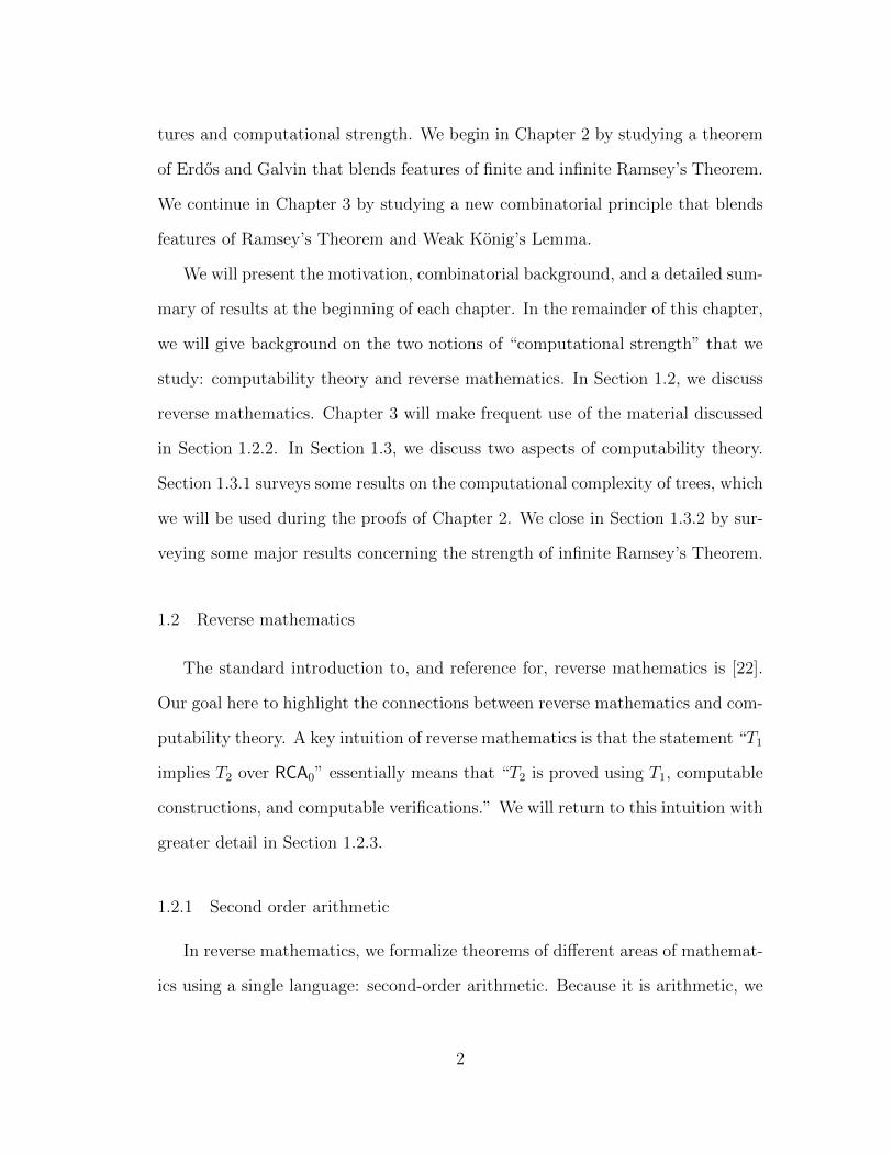
1Figure 3.1. The reverse mathematical strength of RKL.
70
RT32 ACA0 PRT3
5
PRT23
RKL(<ω)
RT22
D<ω2
RKL(1) WKL0
SRT22
RKL
RT1<ω
DNR
RCA0
1
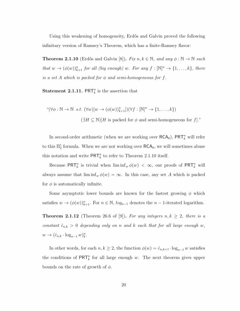
Figure 3.2. The reverse mathematical strength of RKL and PRT.
71
BIBLIOGRAPHY
1. Peter A. Cholak, Carl G. Jockusch, Jr., and Theodore A. Slaman, On thestrength of Ramsey’s theorem for pairs, J. Symbolic Logic 66 (2001), no. 1,1–55.
2. , Corrigendum to: “On the strength of Ramsey’s theorem for pairs”,J. Symbolic Logic 74 (2009), no. 4, 1438–1439.
3. C. T. Chong, personal communication, 2012.
4. C. T. Chong, Steffen Lempp, and Yue Yang, On the role of the collectionprinciple for Σ0
2-formulas in second-order reverse mathematics, Proc. Amer.Math. Soc. 138 (2010), no. 3, 1093–1100.
5. Rod Downey, Denis R. Hirschfeldt, Steffen Lempp, and Reed Solomon, A ∆02
set with no infinite low subset in either it or its complement, J. Symbolic Logic66 (2001), no. 3, 1371–1381.
6. Rod Downey and Carl G. Jockusch, Jr., Effective presentability of Booleanalgebras of Cantor-Bendixson rank 1, J. Symbolic Logic 64 (1999), no. 1,45–52.
7. Damir D. Dzhafarov, Stable Ramsey’s theorem and measure, Notre Dame J.Form. Log. 52 (2011), no. 1, 95–112.
8. Paul Erdos and Fred Galvin, Some Ramsey-type theorems, Discrete Math. 87(1991), no. 3, 261–269.
9. Paul Erdos, Andras Hajnal, Attila Mate, and Richard Rado, Combinatorial settheory: partition relations for cardinals, Studies in Logic and the Foundationsof Mathematics, vol. 106, North-Holland Publishing Co., Amsterdam, 1984.
10. Stephen Flood, Reverse mathematics and a Ramsey-type Konig’s lemma, toappear in the Journal of Symbolic Logic.
72
11. Denis R. Hirschfeldt, Carl G. Jockusch, Jr., Bjørn Kjos-Hanssen, SteffenLempp, and Theodore A. Slaman, The strength of some combinatorial prin-ciples related to Ramsey’s theorem for pairs, Computational prospects of in-finity. Part II. Presented talks, Lect. Notes Ser. Inst. Math. Sci. Natl. Univ.Singap., vol. 15, World Sci. Publ., Hackensack, NJ, 2008, pp. 143–161.
12. Denis R. Hirschfeldt and Richard A. Shore, Combinatorial principles weakerthan Ramsey’s theorem for pairs, J. Symbolic Logic 72 (2007), no. 1, 171–206.
13. Jeffry L. Hirst, A survey of the reverse mathematics of ordinal arithmetic,Reverse Mathematics 2001, Lecture Notes in Logic, vol. 12, Association ofSymbolic Logic, 2005.
14. Jeffry Lynn Hirst, Combinatorics in Subsystems of Second Order Arithmetic,ProQuest LLC, Ann Arbor, MI, 1987, Thesis (Ph.D.)–The Pennsylvania StateUniversity.
15. Carl Jockusch and Frank Stephan, A cohesive set which is not high, Math.Logic Quart. 39 (1993), no. 4, 515–530.
16. Carl G. Jockusch, Jr., Ramsey’s theorem and recursion theory, J. SymbolicLogic 37 (1972), 268–280.
17. , Π01 classes and Boolean combinations of recursively enumerable sets,
J. Symbolic Logic 39 (1974), 95–96.
18. Carl G. Jockusch, Jr. and Robert I. Soare, Π01 classes and degrees of theories,
Trans. Amer. Math. Soc. 173 (1972), 33–56.
19. Jiayi Liu, RT 22 does not imply WKL, J. Symbolic Logic 77 (2012), no. 2,
609–620.
20. Frank P. Ramsey, On a problem of formal logic, Proc. London Math. Soc(1930), no. 30, 264–286.
21. David Seetapun and Theodore A. Slaman, On the strength of Ramsey’s the-orem, Notre Dame J. Formal Logic 36 (1995), no. 4, 570–582, Special Issue:Models of arithmetic.
22. Stephen G. Simpson, Subsystems of second order arithmetic, second ed., Per-spectives in Logic, Cambridge University Press, Cambridge, 2009.
23. Robert I. Soare, Recursively enumerable sets and degrees, Perspectives inMathematical Logic, Springer-Verlag, Berlin, 1987.
73
24. A. S. Troelstra and H. Schwichtenberg, Basic proof theory, Cambridge Tractsin Theoretical Computer Science, vol. 43, Cambridge University Press, Cam-bridge, 1996.
25. Keita Yokoyama, personal communication, 2011.
This document was prepared & typeset with pdfLATEX, and formatted withnddiss2ε classfile (v3.0[2005/07/27]) provided by Sameer Vijay.
74