A more powerful subvector Anderson and Rubin test in linear instrumental variables regression Patrik Guggenberger Pennsylvania State University Joint work with Frank Kleibergen (University of Amsterdam) and Sophocles Mavroeidis (University of Oxford) Indiana University September, 2018
Transcript
A more powerful subvector Anderson and Rubin testin linear instrumental variables regression
Patrik Guggenberger
Pennsylvania State University
Joint work with Frank Kleibergen (University of Amsterdam) and
Sophocles Mavroeidis (University of Oxford)
Indiana University
September, 2018
Overview
• Robust inference on a slope coeffi cient(s) in a linear IV regression
• "Robust" means uniform control of null rejection probability over all "em-pirically relevant" parameter constellations
• "Weak instruments"
— pervasive in applied research (Angrist and Krueger, 1991)
— adverse effect on estimation and inference (Dufour, 1997; Staiger andStock 1997)
• Large literature on "robust inference" for the full parameter vector
• Here: Consider subvector inference in the linear IV model, allowing forweak instruments
• First assume homoskedasticity
— then relax to general Kronecker-Product structure
— then allow for arbitrary forms of heteroskedasticity
• Presentation based on two papers; one being "A more powerful subvectorAnderson Rubin test in linear instrumental variables regression"
• Focus on the Anderson and Rubin (AR, 1949) subvector test statistic:
— "History of critical values":
— Projection of AR test (Dufour and Taamouti, 2005)
— Guggenberger, Kleibergen, Mavroeidis, and Chen (2012, GKMC) pro-vide power improvement:
Using χ2k−mW ,1−α as critical value, rather than χ
2k,1−α still controls
asymptotic size
"Worst case" occurs under strong identification
• HERE: consider a data-dependent critical value that adapts to strengthof identification
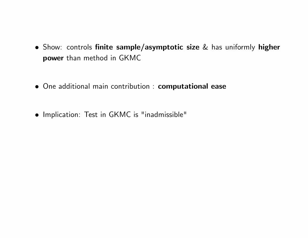
• Show: controls finite sample/asymptotic size & has uniformly higherpower than method in GKMC
• One additional main contribution : computational ease
• Implication: Test in GKMC is "inadmissible"
Presentation
• Introduction: X
• finite sample case
a) mW = 1 : motivation, correct size, power analysis (near optimalityresult)
b) mW > 1 : correct size, uniform power improvement over GKMC
c) refinement
• asymptotic case:
a) homoskedasticity
b) general Kronecker-Product structure
c) general case (arbitrary forms of heteroskedasticity)
Model and Objective (finite sample case)
y = Y β +Wγ + ε,
Y = ZΠY + VY ,
W = ZΠW + VW ,
y ∈ Rn, Y ∈ Rn×mY (end or ex),W ∈ Rn×mW (end), Z ∈ Rn×k (IVs)
• Reduced form:
(y ... Y ... W ) = Z (ΠY... ΠW )
(β
γ...ImY
0...
0
ImW
)+ (vy
... VY... VW )︸ ︷︷ ︸
V
,
where vy := ε+ VY β + VWγ.
• Objective: test
H0 : β = β0 versus H1 : β 6= β0.
s.t. size bounded by nominal size & "good" power
Parameter space:
1. The reduced form error satisfies:
Vi ∼ i.i.d. N (0,Ω) , i = 1, ..., n,
for some Ω ∈ R(m+1)×(m+1) s.t. the variance matrix of (Y 0i, V′Wi)′ for
Y 0i = yi − Y ′i β0 = W ′iγ + εi, namely
Ω (β0) =
1 0−β0 0
0 ImW
′
Ω
1 0−β0 0
0 ImW
is known and positive definite.
2. Z ∈ Rn×k fixed, and Z′Z > 0 k × k matrix.
• Note: no restrictions on reduced form parameters ΠY and ΠW → allowfor weak IV
• Several robust tests available for full vector inference
H0 : β = β0, γ = γ0 vs H1 : not H0
including AR (Anderson and Rubin, 1949), LM, and CLR tests, see Kleiber-gen (2002), Moreira (2003, 2009).
• Optimality properties: Andrews, Moreira, and Stock (2006), Andrews,Marmer, and Yu (2018), and Chernozhukov, Hansen, and Jansson (2009)
Subvector procedures
• Projection: "inf" test statistic over parameter not under test, same criticalvalue → "computationally hard" and "uninformative"
• Bonferroni and related techniques: Staiger and Stock (1997), Chaud-huri and Zivot (2011), McCloskey (2012), Zhu (2015), Andrews (2017),Wangand Tchatoka (2018) ...; often computationally hard, power ranking withprojection unclear
• Plug-in approach: Kleibergen (2004), Guggenberger and Smith (2005)...Re-quires strong identification of parameters not under test.
• GMM models: Andrews, I. and Mikusheva (2016)
• Models defined by moment inequalities: Gafarov (2016), Kaido, Molinari,and Stoye (2016), Bugni, Canay, and Shi (2017), ...
The Anderson and Rubin (1949) test
• AR test stat for full vector hypothesis
H0 : β = β0, γ = γ0 vs H1 : not H0
• AR statistic exploits EZiεi = 0
• AR test stat:
ARn(β0, γ0) =(y − Y β0 −Wγ0)′PZ(y − Y β0 −Wγ0)(
1 ... − β′0... − γ′0
)Ω(
1 ... − β′0... − γ′0
)′
• AR stat is distri. as χ2k under null hypothesis; critical value χ
2k,1−α
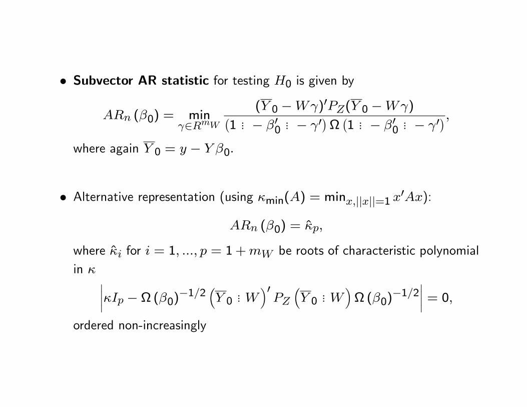
• Subvector AR statistic for testing H0 is given by
ARn (β0) = minγ∈RmW
(Y 0 −Wγ)′PZ(Y 0 −Wγ)(1 ... − β′0
... − γ′)
Ω(1 ... − β′0
... − γ′),
where again Y 0 = y − Y β0.
• Alternative representation (using κmin(A) = minx,||x||=1 x′Ax):
ARn (β0) = κp,
where κi for i = 1, ..., p = 1 +mW be roots of characteristic polynomialin κ ∣∣∣∣κIp − Ω (β0)−1/2
(Y 0
... W)′PZ
(Y 0
... W)
Ω (β0)−1/2∣∣∣∣ = 0,
ordered non-increasingly
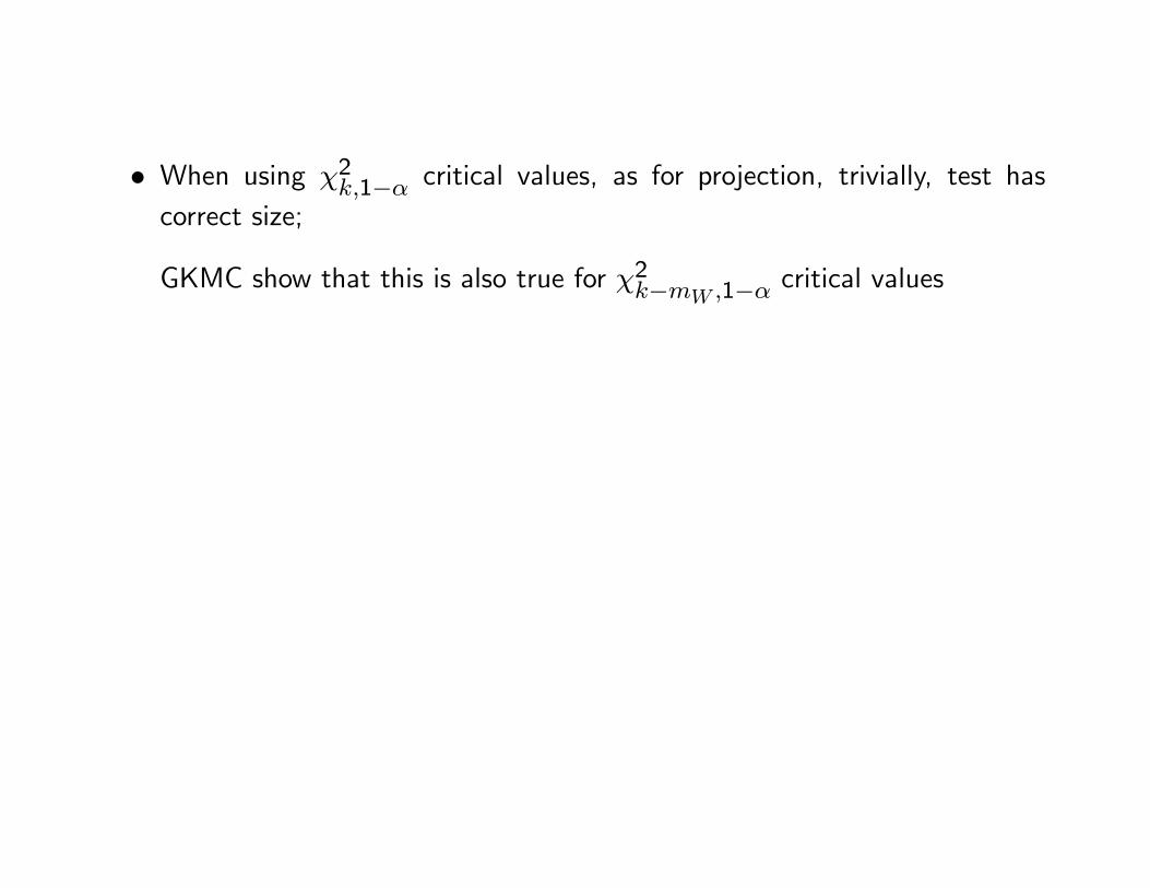
• When using χ2k,1−α critical values, as for projection, trivially, test has
correct size;
GKMC show that this is also true for χ2k−mW ,1−α critical values
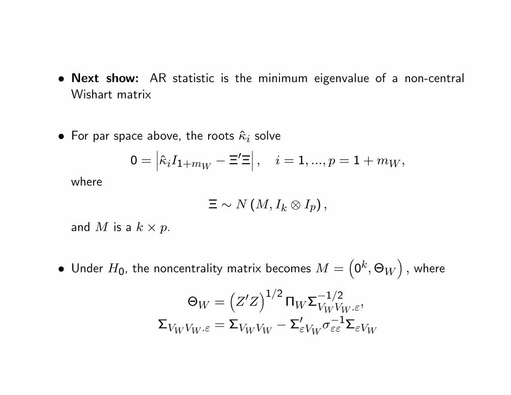
• Next show: AR statistic is the minimum eigenvalue of a non-centralWishart matrix
• For par space above, the roots κi solve
0 =∣∣∣κiI1+mW
− Ξ′Ξ∣∣∣ , i = 1, ..., p = 1 +mW ,
where
Ξ ∼ N (M, Ik ⊗ Ip) ,
and M is a k × p.
• Under H0, the noncentrality matrix becomes M =(
0k,ΘW
), where
ΘW =(Z′Z
)1/2ΠWΣ
−1/2VWVW .ε
,
ΣVWVW .ε = ΣVWVW − Σ′εVWσ−1εε ΣεVW
and (σεε ΣεVW
Σ′εVW ΣVWVW
)=
1 0−β0 0−γ ImW
′
Ω
1 0−β0 0−γ ImW
• Summarizing, under H0 the p× p matrix
Ξ′Ξ ∼W(k, Ip,M
′M),
has non-central Wishart with noncentrality matrix
M ′M =
(0 00 Θ′WΘW
)and
ARn (β0) = κmin(Ξ′Ξ)
• The distribution of the eigenvalues of a noncentral Wishart matrix onlydepends on the eigenvalues of the noncentrality matrix M ′M .
• Hence, distribution of κi only depends on the eigenvalues of Θ′WΘW , κisay, i = 1, . . . ,mW and κ = (κ1, ..., κmW )′
• When mW = 1, κ = κ1 = Θ′WΘW is scalar.
Figure 1: The cdf of the subset AR statistic with k = 3 instruments, fordifferent values of κ1 = 5, 10, 15, 100
Theorem: Suppose mW = 1. Then, under the null hypothesis H0 : β = β0,the distribution function of the subvector AR statistic, ARn (β0) , is monoton-ically decreasing in the parameter κ1.
New critical value for subvector Anderson and Rubin test: mW = 1
• Relevance: If we knew κ1 we could implement the subvector AR test witha smaller critical value than χ2
k−mW ,1−α which is the critical value in thecase when κ1 is "large".
• Muirhead (1978): Under null, when κ1 "is large", the larger root κ1 (whichmeasures strength of identification) is a suffi cient statistic for κ1
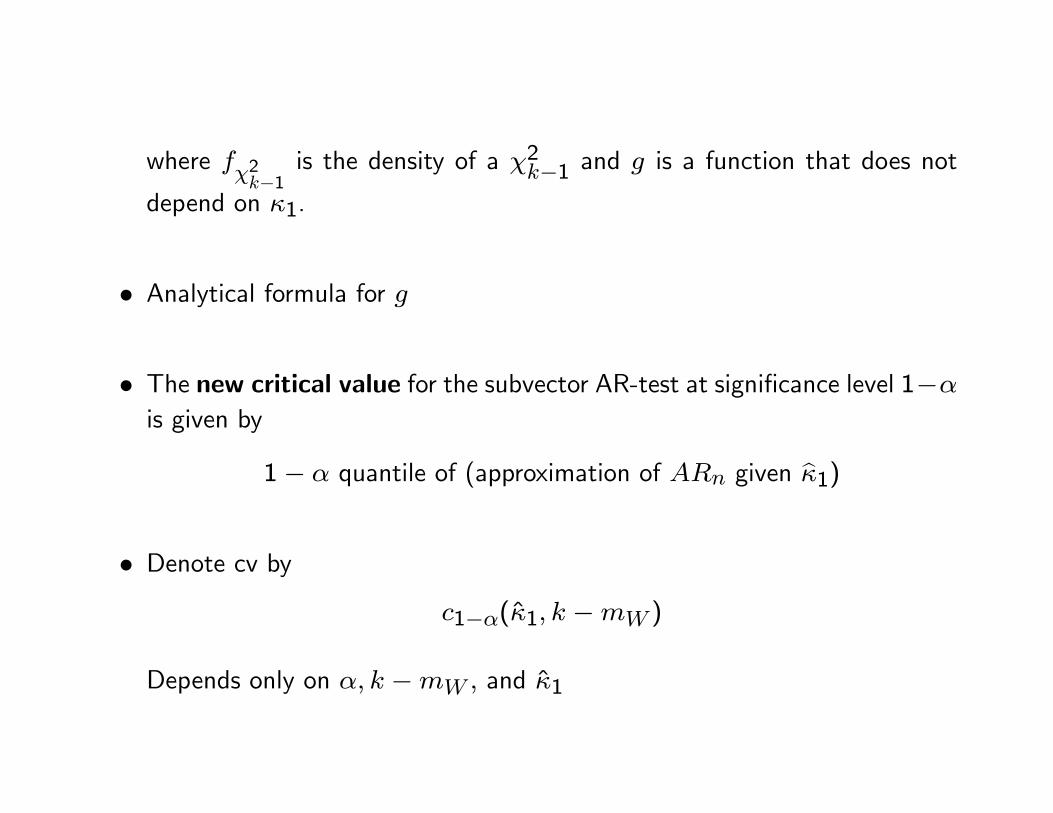
• More precisely: the conditional density of ARn (β0) = κ2 given κ1 canbe approximated by
fκ2|κ1(x) ∼ fχ2
k−1(x) (κ1 − x)1/2 g (κ1) ,
where fχ2k−1
is the density of a χ2k−1 and g is a function that does not
depend on κ1.
• Analytical formula for g
• The new critical value for the subvector AR-test at significance level 1−αis given by
1− α quantile of (approximation of ARn given κ1)
• Denote cv by
c1−α(κ1, k −mW )
Depends only on α, k −mW , and κ1
• Conditional quantiles can be computed by numerical integration
• Conditional critical values can be tabulated→ implementation of new testis trivial and fast
• They are increasing in κ1 and converging to quantiles of χ2k−1
• We find, by simulations over fine grid of values of κ1, that new test
1(ARn (β0) > c1−α(κ1, k −mW ))
controls size
• It improves on the GKMC procedure in terms of power
• Theorem: Suppose mW = 1. The new conditional subvector AndersonRubin test has correct size under the assumptions above.
• Proof partly based on simulations; Verified for e.g. α ∈ 1%, 5%, 10%and k −mW ∈ 1, ..., 20 .
• Summary mW = 1: the cond’l test rejects when
κ2 > c1−α(κ1, k − 1),
where (κ1, κ2) are the eigenvalues of 2×2matrix Ξ′Ξ ∼W(k, Ip,M ′M
);
Under the null M ′M is of rank 1; test has size α
0.1 0.2 1 2 3 10 20 100
1
2
3
4 k = 2
χ 2k − 1 , 1 − α
c 1 − α ( κ 1 ,k − 1 )
0.1 0.2 1 2 3 10 20 100
5
10 k = 5
1 2 3 10 20 100 200
5
10
15
k = 10
1 2 3 4 10 20 100 200
10
20
30k = 20
Critical value function c1−α (κ1, k − 1) for α = 0.05.
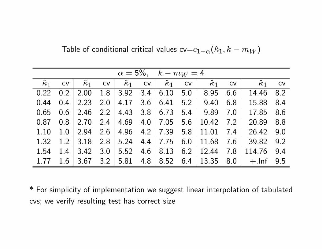
Table of conditional critical values cv=c1−α(κ1, k −mW )
* For simplicity of implementation we suggest linear interpolation of tabulatedcvs; we verify resulting test has correct size
c GKMC
0 10 20 30 40 50 60 70 80 90 100
0.005
0.010
0.015
0.020
0.025
0.030
0.035
0.040
0.045
0.050 k = 5 , m W = 1 , α = 0 .0 5
κ 1
c GKMC
Null rejection frequency of subset AR test based on conditional (red) andχ2k−1 (blue) critical values, as function of κ1.
Extension to mW > 1
We define a new subvector Anderson Rubin test that rejects when
ARn (β0) > c1−α(κmax
(Ξ′Ξ
), k −mW ).
Note: We condition on the LARGEST eigenvalue of the Wishart matrix.
Theorem: The test above has i) correct size and ii) has uniformly largerpower than the test in GKMC.
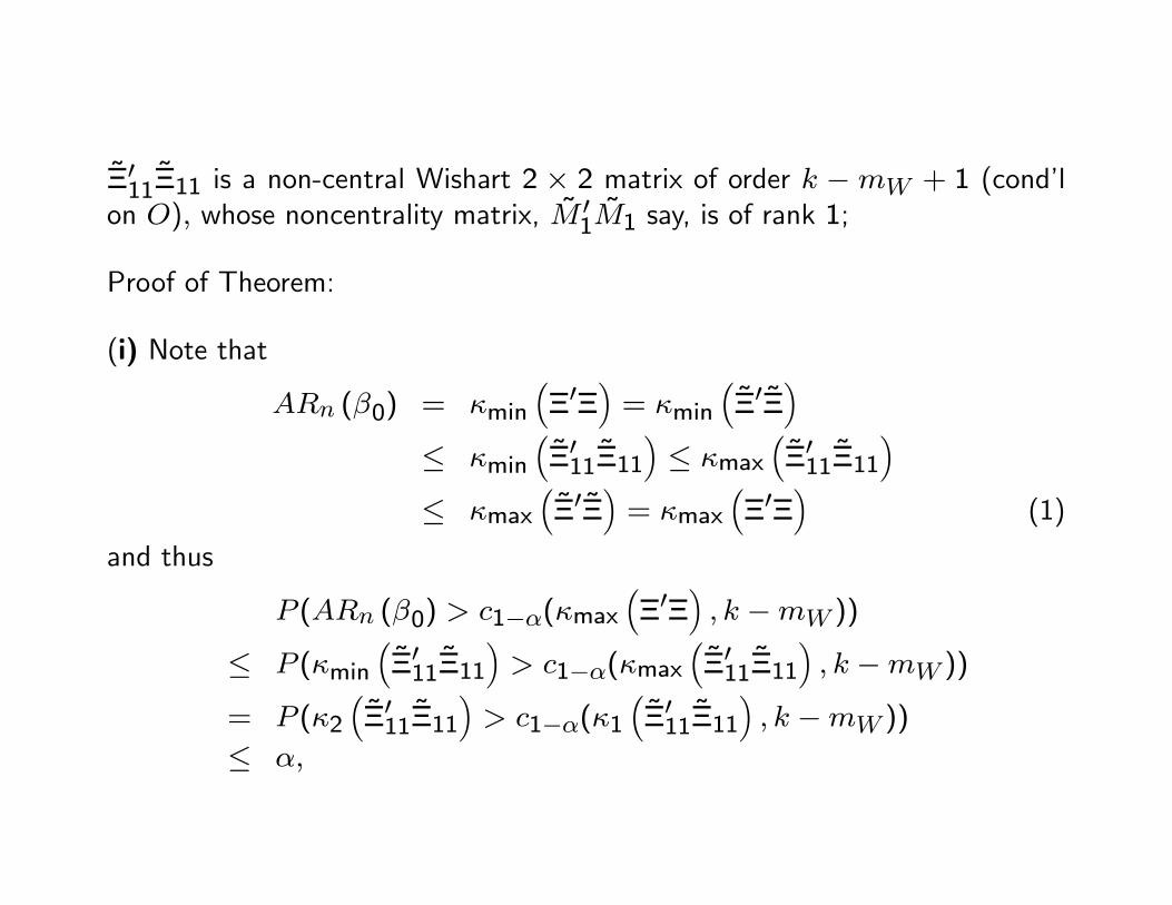
Lemma: Under the nullH0 : β = β0, there exists a random matrix O ∈ O(p),
such that for
Ξ := ΞO ∈ Rk×p, and its upper left submatrix Ξ11 ∈ Rk−mW+1×2
Ξ′11Ξ11 is a non-central Wishart 2 × 2 matrix of order k −mW + 1 (cond’lon O), whose noncentrality matrix, M ′1M1 say, is of rank 1;
Proof of Theorem:
(i) Note that
ARn (β0) = κmin
(Ξ′Ξ
)= κmin
(Ξ′Ξ
)≤ κmin
(Ξ′11Ξ11
)≤ κmax
(Ξ′11Ξ11
)≤ κmax
(Ξ′Ξ
)= κmax
(Ξ′Ξ
)(1)
and thus
P (ARn (β0) > c1−α(κmax
(Ξ′Ξ
), k −mW ))
≤ P (κmin
(Ξ′11Ξ11
)> c1−α(κmax
(Ξ′11Ξ11
), k −mW ))
= P (κ2
(Ξ′11Ξ11
)> c1−α(κ1
(Ξ′11Ξ11
), k −mW ))
≤ α,
where first inequality follows from (1) and last inequality from correct size formW = 1 (by conditionning on O) and the lemma
Recall summary when mW = 1: new test rejects when
κ2 > c1−α(κ1, k − 1)
where (κ1, κ2) are the eigenvalues of Ξ′Ξ ∼W(k, I2,M
′M)and M ′M is of
rank 1 under the null
(ii) new conditional test is uniformly more powerful than test in GKMC (becausec1−α(·, k −mW )) is increasing and converging to χ2
k−mW ,1−α as argumentgoes to infinity), i.e. the test in GKMC is inadmissible
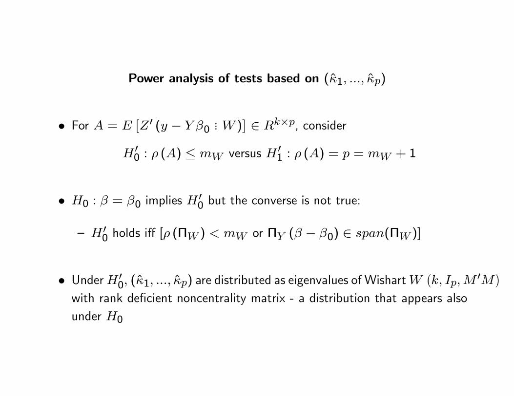
Power analysis of tests based on (κ1, ..., κp)
• For A = E[Z′ (y − Y β0
... W )]∈ Rk×p, consider
H ′0 : ρ (A) ≤ mW versus H ′1 : ρ (A) = p = mW + 1
• H0 : β = β0 implies H′0 but the converse is not true:
— H ′0 holds iff [ρ (ΠW ) < mW or ΠY (β − β0) ∈ span(ΠW )]
• UnderH ′0, (κ1, ..., κp) are distributed as eigenvalues of WishartW(k, Ip,M ′M
)with rank deficient noncentrality matrix - a distribution that appears alsounder H0
• Thus, every test ϕ(κ1, ..., κp) ∈ [0, 1] that has size α under H0 mustalso have size α under H ′0 - so cannot have power exceeding size underalternatives H ′0\H0.
• In other words, size α tests ϕ(κ1, ..., κp) underH0 can only have nontrivialpower under alternatives ρ (A) = p.
• We use this insight to derive a power envelope for tests of the formϕ (κ1, ..., κp) .
Power bounds
• Consider only the case mW = 1.
• Equivalently, H ′0 : κ2 = 0, κ1 ≥ κ2 against H ′1 : κ2 > 0, κ1 ≥ κ2.
• Obtain point-optimal power bounds using approximately least favorabledistribution ΛLF over nuisance parameter κ1 based on algorithm in Elliott,Müller, and Watson (2015)
P o we r o f ϕ c m inus po wer bo und
κ 2
κ1 − κ
2
10 20 3025
5075
0.0
20
.01
0
p ow er boundϕ cϕ G K M C
0 5 1 0 1 5 2 0 2 5 3 0
0 .5
1 .0 P o wer curves when κ 1 = κ 2
κ 2
p ow er boundϕ cϕ G K M C
Power of conditional subvector AR test ϕc (κ) = 1κ2>c1−α(κ1,k−1) relative to powerbound (left) and power of ϕc, ϕGKMC (κ) = 1
κ2>χ2k−1,1−α
= 1κ2>c1−α(∞,k−1)
and bound at κ1 = κ2 (right) for k = 5. Computed using 10000 MC replications.
• Little scope for power improvement over proposed test. But not zeroscope...:
Refinement: For the case k = 5, mW = 1, and α = 5%, let ϕadj be the testthat uses the critical values in Table above where the smallest 8 critical valuesare divided by 5
Asymptotic case: a) homoskedasticity
• Define parameter space F under the null hypothesis H0 : β = β0.
Let Ui := (εi + V ′W,iγ, V′W,i)
′ and F distribution of (Ui, VY i, Zi)
F is set of all (γ,ΠW ,ΠY , F ) s.t.
γ ∈ RmW ,ΠW ∈ Rk×mW ,ΠY ∈ Rk×mY ,
EF (||Ti||2+δ) ≤M, for Ti ∈ vec(ZiUi), Zi, Ui,EF (Zi(εi, V
′Wi, V
′Y i)) = 0,
EF (vec(ZiU′i)(vec(ZiU
′i))′) = (EF (UiU
′i)⊗ EF (ZiZ
′i)),
κmin(A) ≥ δ for A ∈ EF (ZiZ′i), EF (UiU
′i)
for some δ > 0, M <∞
• Note: no restriction is imposed on the variance matrix of vec(ZiV ′Y i)
• subvector AR stat equals smallest solution of∣∣∣∣∣∣κI1+mW− (
Y′MZY
n− k)−1/2(Y
′PZY )(
Y′MZY
n− k)−1/2
∣∣∣∣∣∣ = 0
where
Y := (y − Y β0... W ) ∈ Rn×(1+mW )
• Note: Same as in finite sample case with Ω (β0) replaced by Y′MZYn−k
• critical value is again
c1−α(κ1, k −mW )
the 1− α quantile of (the approximation of) ARn given κ1
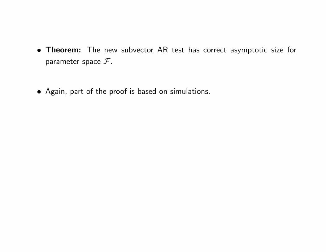
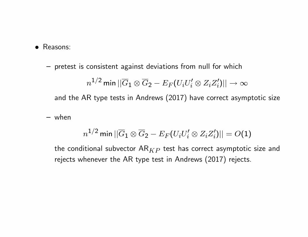
• Theorem: The new subvector AR test has correct asymptotic size forparameter space F .
• Again, part of the proof is based on simulations.
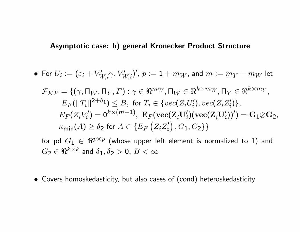
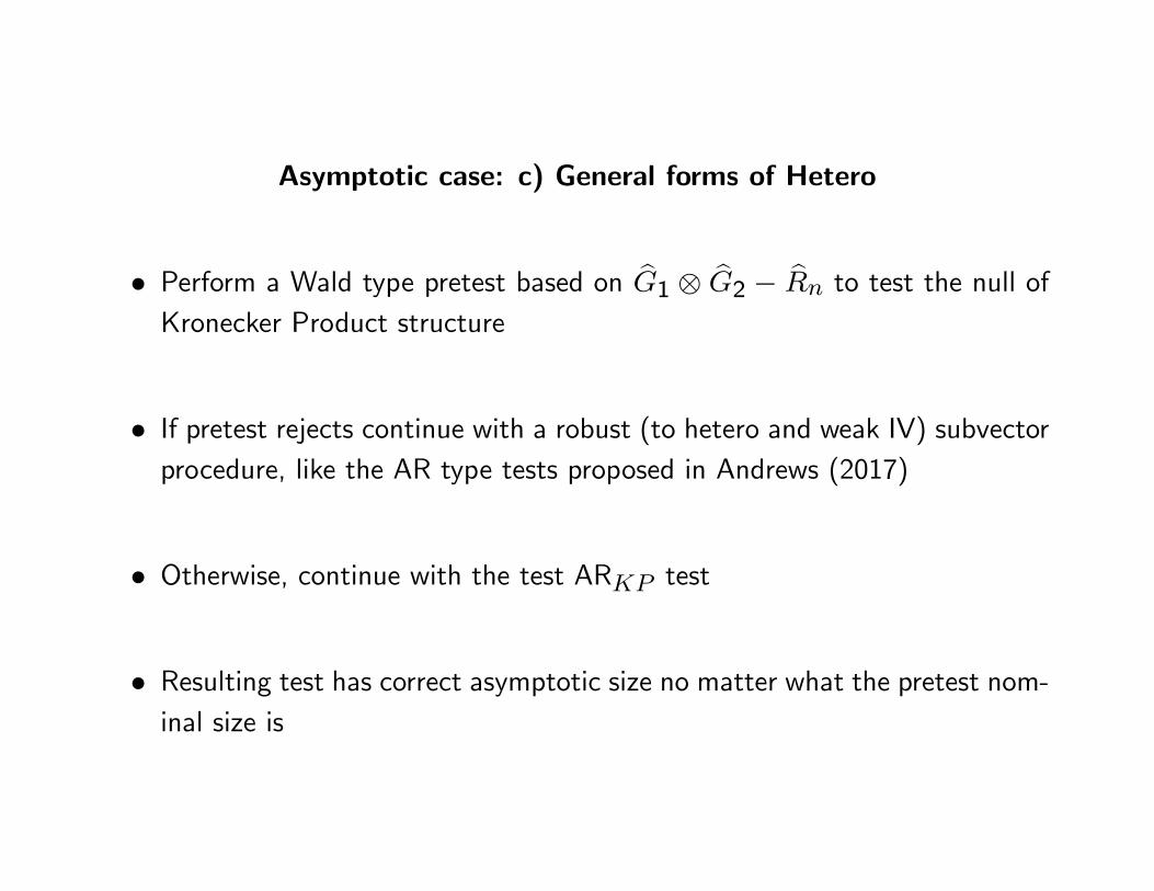
Asymptotic case: b) general Kronecker Product Structure
EF (||Ti||2+δ1) ≤ B, for Ti ∈ vec(ZiU ′i), vec(ZiZ′i),EF (ZiV
′i ) = 0k×(m+1), EF (vec(ZiU
′i)(vec(ZiU
′i))′) = G1⊗G2,
κmin(A) ≥ δ2 for A ∈ EF(ZiZ
′i
), G1, G2
for pd G1 ∈ <p×p (whose upper left element is normalized to 1) andG2 ∈ <k×k and δ1, δ2 > 0, B <∞
• Covers homoskedasticity, but also cases of (cond) heteroskedasticity
Example. Take (εi, V′Wi)′ ∈ <p i.i.d. zero mean with pd variance matrix,
independent of Zi, and
(εi, V′Wi)′ := f(Zi)(εi, V
′Wi)′
for some scalar valued function f of Z, e.g. f(Zi) = ||Zi||/k1/2. Then
EF (vec(ZiU′i)(vec(ZiU
′i))′)
=EF(UiU
′i ⊗ ZiZ′i
)=EF
((εi + V ′W,iγ, V
′W,i)
′(εi + V ′W,iγ, V′W,i)⊗ ZiZ
′i
)=EF
((εi + V ′W,iγ, V
′W,i)
′(εi + V ′W,iγ, V′W,i)
)⊗ EF
(f(Zi)
2ZiZ′i
)has KP structure even though
EF (UiU′i|Zi) = f(Zi)
2EF (εi + V ′W,iγ, V′W,i)
′(εi + V ′W,iγ, V′W,i)
depends on Zi.
• Modified AR subvector statistic. Estimate EF (UiU′i ⊗ ZiZ′i) by
Rn := n−1n∑i=1
fif′i ∈ <kp×kp, where
fi := ((MZ(y − Y β0))i, (MZW )′i)′ ⊗ Zi ∈ <kp.
• Let
(G1, G2) = arg min ||G1 ⊗G2 − Rn||F ,
where the minimum is taken over (G1, G2) for G1 ∈ <p×p, G2 ∈ <k×kbeing pd, symmetric matrices, normalized such that the upper left elementof G1 equals 1. Estimators are unique and given in closed form.
• The subvector AR statistic, ARKP,n(β0) is defined it as the smallestroot κpn of the roots κin, i = 1, ..., p (ordered nonincreasingly) of the
characteristic polynomial∣∣∣∣κIp − n−1G−1/21
(Y 0,W
)′ZG−1
2 Z′(Y 0,W
)G−1/21
∣∣∣∣ = 0.
• Note: Relative to previous definition,
G1 replacesY′MZYn−k and G2 replaces
Z′Zn
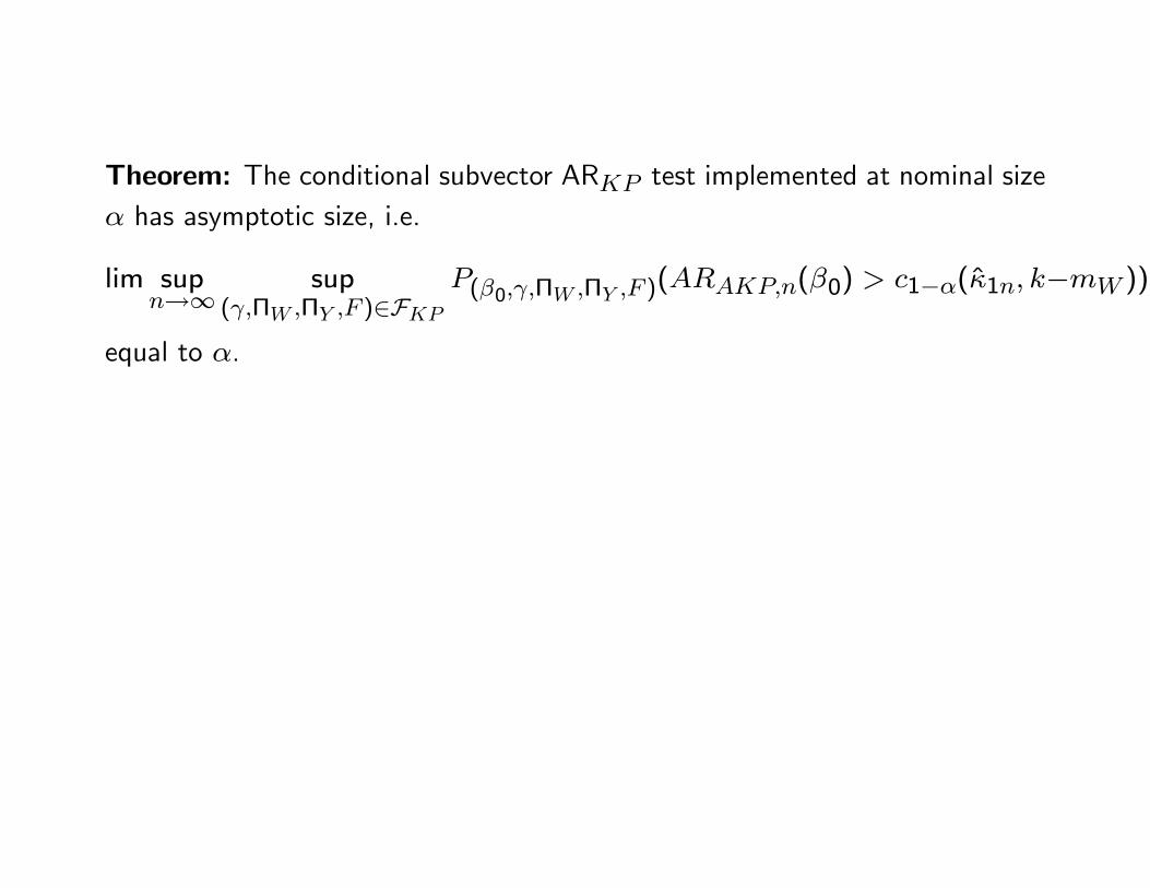
• The conditional subvector ARKP test rejects H0 at nominal size α if
ARKP,n(β0) > c1−α(κ1n, k −mW ),
where c1−α (·, ·) is defined as above.
Theorem: The conditional subvector ARKP test implemented at nominal sizeα has asymptotic size, i.e.
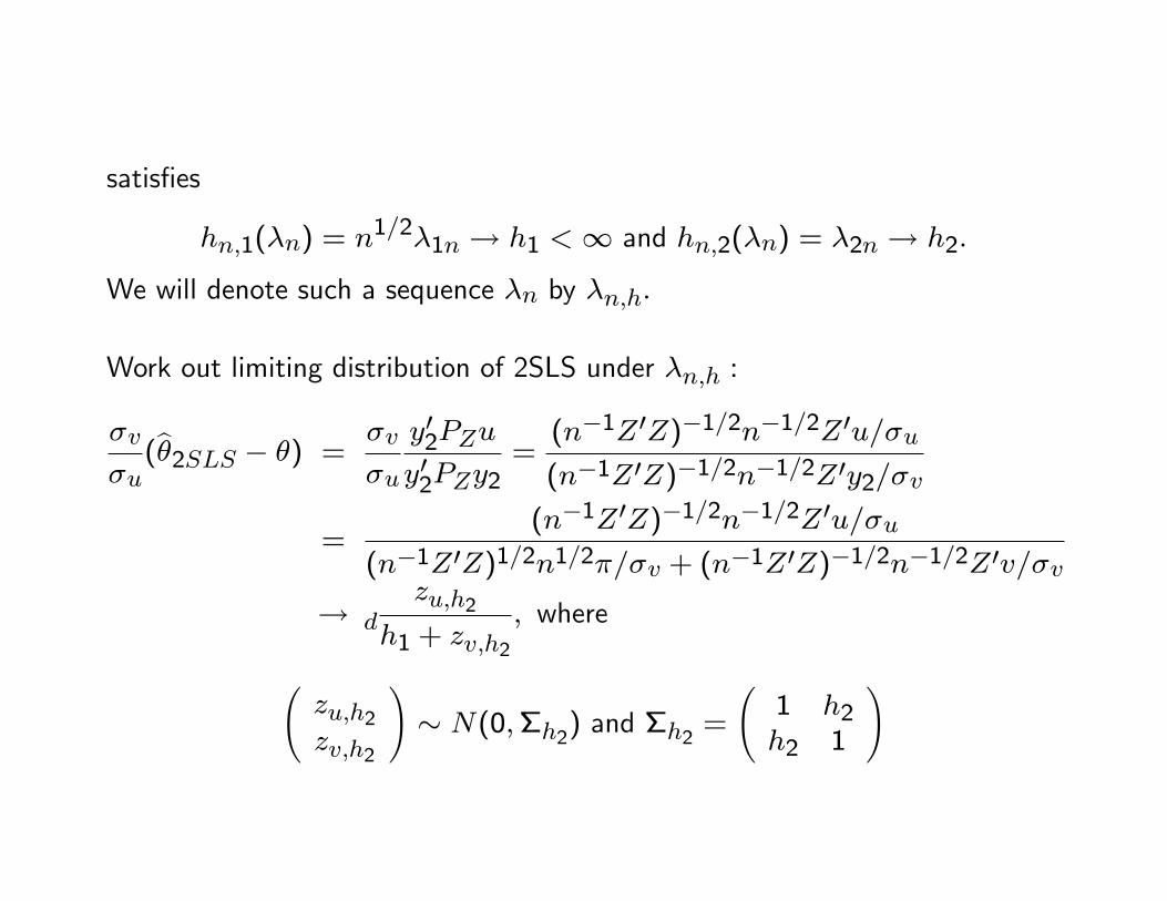
Work out limiting distribution of 2SLS under λn,h :
σv
σu(θ2SLS − θ) =
σv
σu
y′2PZuy′2PZy2
=(n−1Z′Z)−1/2n−1/2Z′u/σu(n−1Z′Z)−1/2n−1/2Z′y2/σv
=(n−1Z′Z)−1/2n−1/2Z′u/σu
(n−1Z′Z)1/2n1/2π/σv + (n−1Z′Z)−1/2n−1/2Z′v/σv
→ dzu,h2
h1 + zv,h2
, where
(zu,h2zv,h2
)∼ N(0,Σh2
) and Σh2=
(1 h2h2 1
)
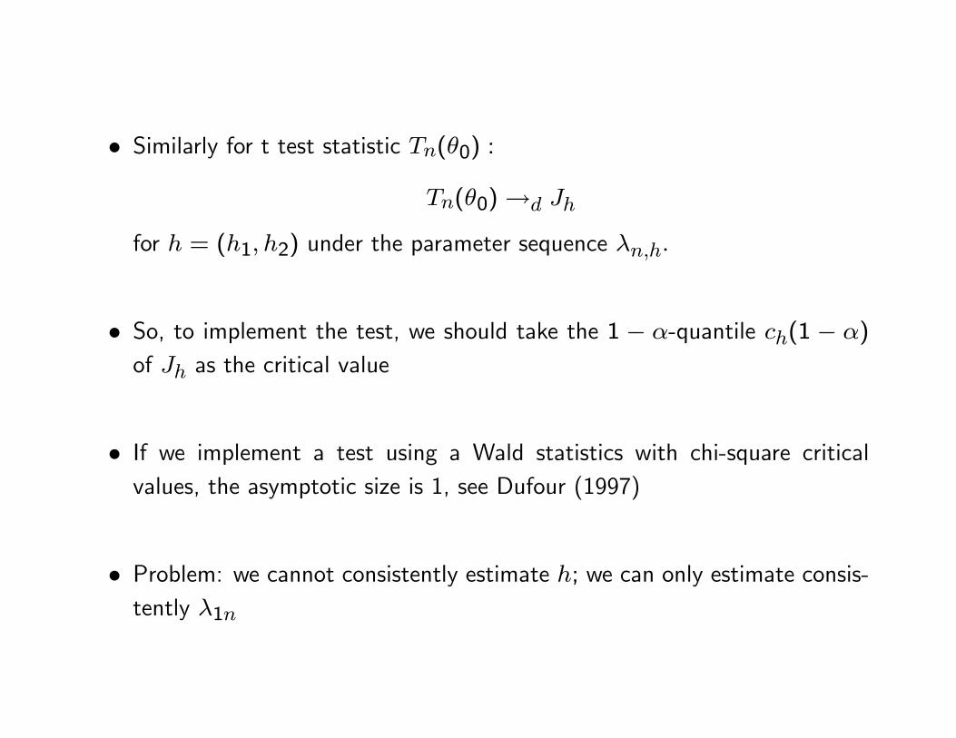
• Similarly for t test statistic Tn(θ0) :
Tn(θ0)→d Jh
for h = (h1, h2) under the parameter sequence λn,h.
• So, to implement the test, we should take the 1 − α-quantile ch(1 − α)
of Jh as the critical value
• If we implement a test using a Wald statistics with chi-square criticalvalues, the asymptotic size is 1, see Dufour (1997)
• Problem: we cannot consistently estimate h; we can only estimate consis-tently λ1n
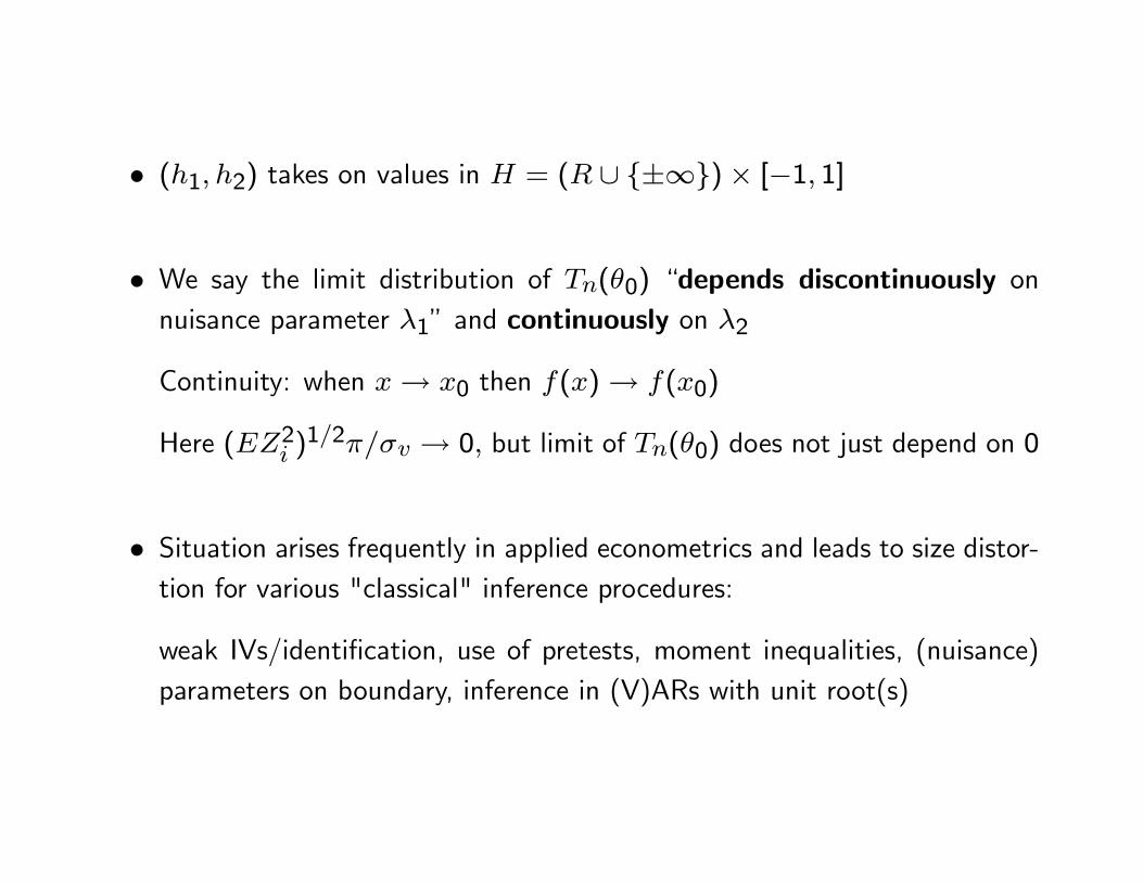
• (h1, h2) takes on values in H = (R ∪ ±∞)× [−1, 1]
• We say the limit distribution of Tn(θ0) “depends discontinuously onnuisance parameter λ1”and continuously on λ2
Continuity: when x→ x0 then f(x)→ f(x0)
Here (EZ2i )1/2π/σv → 0, but limit of Tn(θ0) does not just depend on 0
• Situation arises frequently in applied econometrics and leads to size distor-tion for various "classical" inference procedures:
weak IVs/identification, use of pretests, moment inequalities, (nuisance)parameters on boundary, inference in (V)ARs with unit root(s)
General Theory: Asymptotic Size of Tests
• ϕn : n ≥ 1 sequence of tests for null hypothesis H0
• λ indexes the true null distribution of the observations
• Parameter space for λ is some space Λ
• RPn(λ) denotes rejection probability of ϕn under λ
• The asymptotic size of ϕn for the parameter space Λ is defined as:
AsySz = lim supn→∞
supλ∈Λ
RPn(λ)
Formula for Calculation of AsySzRecall relevance of limits of hn,1(λn) = n1/2λ1n = n1/2(EZ2
i )1/2π/σv andhn,2(λn) = λ2n = corr(ui, vi) for limit distributions of test statistics in weakIV example
Generalizing, let
hn(λ) = (hn,1(λ), ..., hn,J(λ))′ ∈ RJ : n ≥ 1be a sequence of functions on Λ, where hn,j(λ) ∈ R ∀j = 1, ..., J.
For any subsequence pn of n and h ∈ (R ∪ ±∞)J denote a sequenceλpn ∈ Λ : n ≥ 1 such that hpn(λpn)→ h by
λpn,h
Define
H = h ∈ (R∪±∞)J : there is subsequence pn and sequence λpn,h.
Theorem, Andrews, Cheng, and Guggenberger (2011)
Assume that under any sequence λpn,h
RPpn(λpn,h)→ RP (h)
for some RP (h) ∈ [0, 1]. Then:
AsySz = suph∈H
RP (h).
Proof. i) Let h ∈ H. To show AsySz ≥ RP (h). By definition of H, there isλpn,h. Then
AsySz = lim supn→∞
supλ∈Λ
RPn(λ)
≥ lim supn→∞
RPpn(λpn,h)
= RP (h)
Proof. (continued)
ii) To show AsySz ≤ suph∈H RP (h). Let λn ∈ Λ : n ≥ 1 be a sequencesuch that
lim supn→∞
RPn(λn) = AsySz.
Let pn : n ≥ 1 be a subsequence of n such that limn→∞RPpn(λpn)
exists and equals AsySz and hpn(λpn) → h. Therefore this sequence is oftype λpn,h, and thus, by assumption, RPpn(λpn) → RP (h). Because alsoRPpn(λpn)→ AsySz, it follows that AsySz = RP (h).
Specification of λ for subvector Anderson and Rubin test
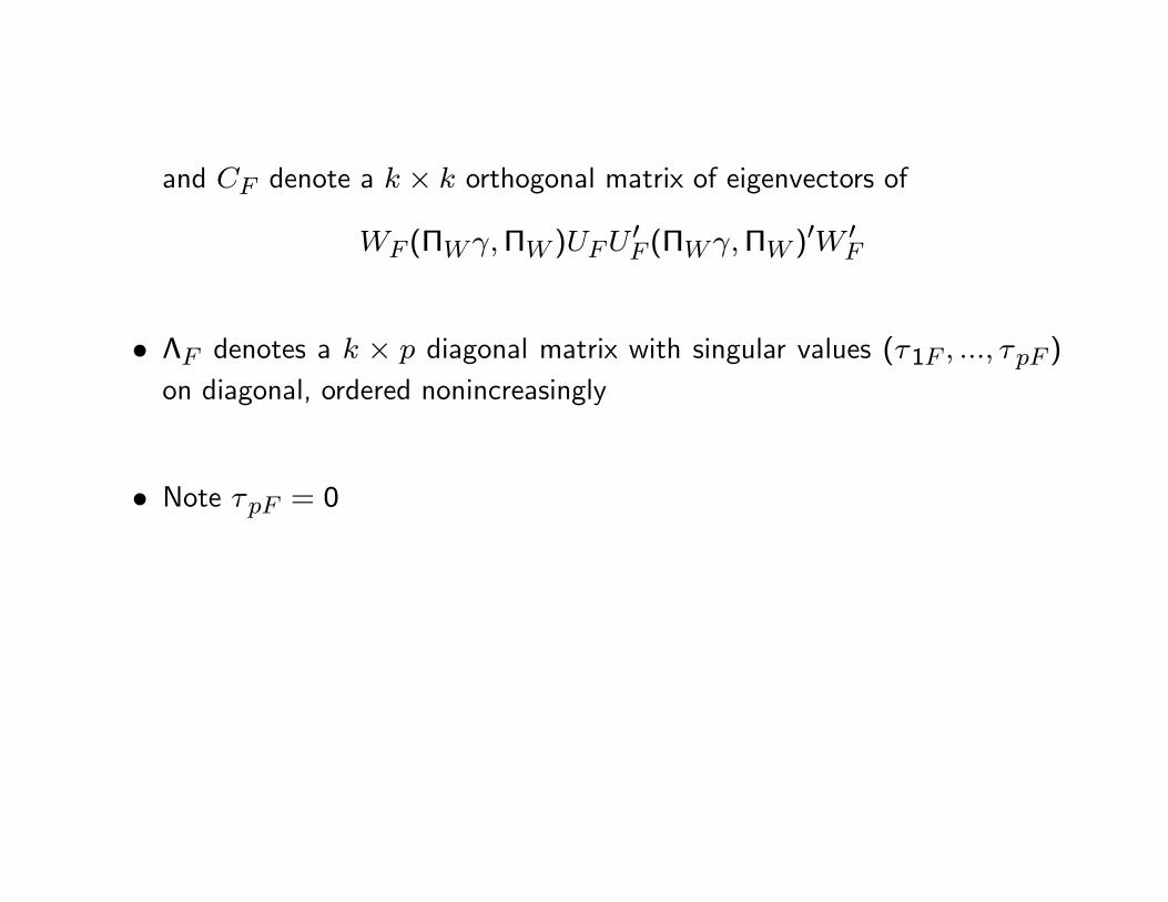
• Given F let
WF := (EFZiZ′i)
1/2 and UF := Ω(β0)−1/2.
• Consider a singular value decomposition
CFΛFB′F
of
WF (ΠWγ,ΠW )UF
• i.e. BF denote a p× p orthogonal matrix of eigenvectors of
U ′F (ΠWγ,ΠW )′W ′FWF (ΠWγ,ΠW )UF
and CF denote a k × k orthogonal matrix of eigenvectors of
WF (ΠWγ,ΠW )UFU′F (ΠWγ,ΠW )′W ′F
• ΛF denotes a k × p diagonal matrix with singular values (τ1F , ..., τpF )
∞ includes some weakly/some strongly ident’d parameters, as in Stock& Wright (2000); also includes joint weak ident’n
Andrews and Guggenberger (2014): Limit distribution of eigenvalues ofquadratic forms
• Consider a singular value decomposition CFΛFB′F of WFDFUF
• Define λF , h, λn,h... as above
Let κjn ∀j = 1, ..., p denote jth eigenval of
nU ′nD′nW
′nWnDnUn,
where under λn,h
n1/2(Dn −DFn) → dDh ∈ Rk×p,Wn −WFn → p0k×k,
Un − UFn → p0p×p,
WFn → h4, UFn → h5
with h4, h5 nonsingular
Theorem (AG, 2014): under λn,h : n ≥ 1,
(a) κjn →p ∞ for all j ≤ q
(b) vector of smallest p−q eigenvals of nU ′nD′nW ′nWnDnUn, i.e., (κ(q+1)n, ..., κpn)′,converges in dist’n to p− q vector of eigenvals of random matrixM(h,Dh) ∈R(p−q)×(p−q)
• complicated proof;— eigenvalues can diverge at any rate or converge to any number— can become close to each other or close to 0 as n→∞
• We apply this result with
WF = (EFZiZ′i)
1/2, Wn = (n−1∑ZiZ′i)
1/2,
UF = Ω(β0)−1/2, Un =
Y ′MZY
n− k
−1/2
,
DF = (ΠWγ,ΠW ), Dn = (Z′Z)−1Z′Y
to obtain the joint limiting distribution of all eigenvalues
Joint asymptotic dist’n of eigenvalues
• Recall: test statistic and critical value are functions of p = 1 +mW rootsof ∣∣∣∣∣∣κI1+mW
− (Y′MZY
n− k)−1/2(Y
′PZY )(
Y′MZY
n− k)−1/2
∣∣∣∣∣∣ = 0
• To obtain joint limiting distribution of eigenvalues, we use general resultin Andrews and Guggenberger (2014) about joint limiting distribution ofeigenvalues of quadratic forms
Results:
• the joint limit depends only on localization parameters h1,1, ..., h1,mW
• asymptotic cases replicate finite sample, normal, fixed IV, known variancematrix setup
• together with above proposition, correct asymptotic size then follows fromcorrect finite sample size