WP GLM|LIC Working Paper No. 42 | March 2018 Patrilocal Residence and Female Labour Supply Andreas Landmann (Paris School of Economics, J-PAL Europe and C4ED) Helke Seitz (DIW and Leibniz University Hannover) Susan Steiner (Leibniz University Hannover and IZA)
Transcript
WP
GLM|LIC Working Paper No. 42 | March 2018
Patrilocal Residence and Female Labour Supply
Andreas Landmann (Paris School of Economics, J-PAL Europe and C4ED)Helke Seitz (DIW and Leibniz University Hannover)Susan Steiner (Leibniz University Hannover and IZA)
GLM|LICc/o IZA – Institute of Labor EconomicsSchaumburg-Lippe-Straße 5–953113 Bonn, Germany
Andreas Landmann (Paris School of Economics, J-PAL Europe and C4ED)Helke Seitz (DIW and Leibniz University Hannover)Susan Steiner (Leibniz University Hannover and IZA)
ABSTRACT
GLM|LIC Working Paper No. 42 | March 2018
Patrilocal Residence and Female Labour Supply*
Many people around the world live in patrilocal societies. Patrilocality prescribes that women move in with their husbands’ parents, relieve their in-laws from housework, and care for them in old age. This arrangement is likely to have labour market consequences, in particular for the women. We study the effect of co-residence on female labour supply in Kyrgyzstan, a strongly patrilocal setting. We account for the endogeneity of co-residence by exploiting the tradition that youngest sons usually live with their parents. In both OLS and IV estimations, the effect of co-residence on female labour supply is negative and insignificant. This is in contrast to previous studies, which found positive effects in less patrilocal settings. We go beyond earlier work by investigating effect channels. In Kyrgyzstan, co-residing women invest more time in elder care than women who do not co-reside and they do not receive parental support in housework.
JEL Classification:J12, J21
Keywords:family structure, co-residence, labour supply, patrilocality, Kyrgyzstan
Corresponding author:Susan SteinerInstitute for Development and Agricultural EconomicsLeibniz Universität HannoverKönigsworther Platz 130167 HannoverGermanyE-mail: [email protected]
* This work was supported by the UK Department for International Development (DFID) and the Institute for the Study of Labor (IZA). It is an output of the project “Gender and Employment in Central Asia - Evidence from Panel Data”. The views expressed are not necessarily those of DFID or IZA. We gratefully acknowledge the financial support received. Andreas Landmann received additional funding from project LA 3936/1-1 of the German Research Foundation (DFG). We thank Kathryn Anderson, Charles M. Becker, Marc Gurgand, Kristin Kleinjans, Patrick Puhani and participants of conferences in Bishkek, Chicago, Dresden and Göttingen for helpful and valuable comments. Many thanks in particular to Damir Esenaliev and Tilman Brück for their support.
1 Introduction
Post-marital residence rules determine where newly wed couples should reside. A
large share of the world population lives in societies with a patrilocal residence rule.1
This rule prescribes that women move in with their husbands’ parents, or sometimes
the husband’s wider family, upon marriage. When joining the new household, women
are usually expected to relieve their in-laws from housework and to care for them in
old age (Grogan, 2013; Ebenstein, 2014). Such co-residence arrangements may have
significant labour market consequences for the involved women. In this study, we
therefore investigate how intergenerational co-residence affects female labour supply
in a patrilocal setting. We focus on Kyrgyzstan where elderly parents traditionally
reside with their youngest son and his wife.
A priori, the impact of intergenerational co-residence on the labour supply of
women is unclear because several channels can be at play and might counteract
each other. The literature has elaborated on four channels through which the im-
pact can principally work. First, co-residing parents or in-laws might contribute to
household income or share housing and other assets (Maurer-Fazio et al., 2011). Any
advantage in economic conditions (e.g. high non-labour income) is likely to make
women reduce their labour supply. Second, co-residing parents or in-laws might re-
quire care. Women are typically the caregivers in the household. This responsibility
increases their value of non-market time (their reservation wage) and reduces their
labour supply (Lilly et al., 2007). Third, co-residing parents or in-laws might take
care of women’s children or take over housekeeping tasks. The reservation wage is re-
duced for the women, leading to an increase in labour supply (Compton and Pollak,
2014; García-Morán and Kuehn, 2017; Posadas and Vidal-Fernández, 2013; Shen
et al., 2016). Fourth, co-residing parents or in-laws might be better able to impose
their preferences on a woman’s labour market behaviour than distant parents or174 percent of societies around the world were traditionally patrilocal (Murdock, 1967, cited in Baker
and Jacobsen, 2007). Today, patrilocality is most common in the Caucasus, Central Asia, and South Asia.The share of elderly co-residing with a son and his wife is particularly high in these societies (Grogan,2013; Ebenstein, 2014).
3
in-laws (Chu et al., 2014). Depending on the type of preferences, parents or in-laws
can either induce an increase or a reduction in female labour supply. These four
channels are plausible in patrilocal societies in the same way as in other societies
- with one exception. Women who move in with their in-laws are assumed to take
over housekeeping tasks from them rather than the in-laws taking care of housekeep-
ing for the women (Grogan, 2013). This distribution of tasks within the household
should result in more adverse effects of co-residence on female labour supply in a
patrilocal context than in a non-patrilocal context.
A simple cross-country analysis illustrates that patrilocal countries are different
from non-patrilocal countries. Figure 1 shows the correlation between female labour
force participation and intergenerational co-residence rates in patrilocal countries
and non-patrilocal countries separately.2 While co-residence is positively related to
female labour force participation in the latter, the correlation is negative in patrilocal
countries. This pattern suggests that the effect of intergenerational co-residence is
distinct, and potentially negative, in patrilocal countries. Yet, cross-country analyses
can hardly provide causal insights. Instead, micro-level investigations are needed.
[Insert Figure 1 about here]
There are only few micro-level studies on labour supply effects of living with the
parent generation (Kolodinsky and Shirey, 2000; Sasaki, 2002; Oishi and Oshio, 2006;
Maurer-Fazio et al., 2011; Shen et al., 2016).3 All these studies find that co-residence
increases female labour supply and claim that this is due to parental assistance
with child care and housekeeping. Yet, most of the authors limit themselves to
speculation; only Shen et al. (2016) explicitly test and confirm this claim for the
case of housework. None of the other channels are analyzed.
In this study, we contribute to the literature by investigating all channels through2The list of countries used for this analysis can be found in Table A.1.3Additionally, Compton (2015) evaluates the effect of proximity to parents on labour market outcomes
of women. She finds that, when controlling for the endogeneity of distance to the parents, close proximityto parents increases the labour force participation of married women. Please note that this study is notfully comparable to the other studies, as it focuses on proximity to parents rather than co-residence withparents.
4
which intergenerational co-residence can potentially affect women’s supply of labour
to the market. We focus on Kyrgyzstan, which is a post-Soviet country in Central
Asia with a population of 5.9 million and where patrilocality is common: 46 percent
of married females in the age group 15-30 live with at least one parent-in-law and only
9 percent live with at least one own parent (Grogan, 2013). Young married women
reportedly have the lowest status in their in-laws’ household (Kuehnast, 2004). They
are supposed to be obedient and to fulfill the demands of their husbands and his
parents. Married couples tend to live with the husband’s parents until the husband’s
younger brothers get married. At that point, they often move out and form their
own household. According to tradition, the youngest son and his wife never move out
and are responsible for the well-being of the parents (Bauer et al., 1997; Kuehnast,
2004; Thieme, 2014; Rubinov, 2014). As a way of compensation, the youngest son
inherits the house and the land upon the death of his father.4
In contrast to the previous literature, we do not only measure the impact of
living with the parent generation on female labour supply; we also shed light on
the channels. With the help of time use data, we can draw conclusions on how
time spent on child care, elder care and housekeeping differs between women who
co-reside and women who do not co-reside. Furthermore, we have information on
income contributed to the household by co-residing parents as well as their attitudes
on gender roles. We correlate this information with female labour supply.
Empirical analysis is not straightforward because co-residence is not exogenous.
Even in patrilocal societies such as Kyrgyzstan, there is selection into co-residence.
Couples that are expected to co-reside with the husband’s parents do not always do
so, while couples that are not necessarily expected to co-reside sometimes decide to
live with the older generation. The reason is that co-residence and labour supply
decisions are often made jointly (Sasaki, 2002). For example, young women with low
ambition to work outside the home or with conservative attitudes on gender roles
may be inclined to co-reside with their in-laws. Additionally, parents are likely to4All children traditionally get a share of the parents’ wealth, though in different forms and at different
times in their life cycle (Giovarelli et al., 2001).
5
move in with their adult children when they need to be taken care of or when the
adult children need them as caregivers for their own children, especially if formal
care is not easily available or too costly. If there are several siblings, the co-residence
decision could be the result of a bargaining process. The sibling with the lowest
(highest) opportunity costs may be the one who co-resides with parents if elder
(child) care is required (Ettner, 1996; Ma and Wen, 2016). Due to this endogeneity
of co-residence, simple comparisons of co-residing and non-co-residing women are
most likely subject to a bias.
To address the endogeneity of co-residence, we make use of the tradition that
youngest sons are expected to live with their parents in Kyrgyzstan. This tradition
stems from nomadic life style historically prevalent in much of Central Asia. It was
due to the space restrictions in yurts (portable tents) but has no economic rele-
vance today. Yet, it has become such an internalized tradition that all ethnic groups
residing in the country, even those without nomadic roots, follow it today.5 It gen-
erates exogenous variation in the co-residence of women with the parent generation,
driven by the birth order of husbands. We use being married to the youngest son to
construct an instrument for women’s intergenerational co-residence. We show that
wives of youngest sons are significantly and substantially more likely to co-reside
than otherwise comparable wives of older sons. Several tests suggest plausibility of
the instrument: Youngest sons do not seem to differ from older sons with regard to
pre-marriage characteristics and divorce rates. The same holds for their wives.
We find that the patrilocal setting in Kyrgyzstan is different from the settings
investigated in the previous literature, as reflected in the deviating overall effect of
co-residence on female labour supply. In Kyrgyzstan, co-residence does not signif-5According to information obtained in expert interviews, it was the parents’ duty in Turkic and Mon-
golian nomadic cultures to allocate a certain number of livestock to their older sons when they got marriedand to separate them by giving them a yurt. Keeping the sons and their wives in the parents’ yurt wouldhave been impossible due to space restrictions. When parents died, it was the youngest son’s duty to burythe parents. In return, he inherited the parents’ yurt and their remaining livestock. This tradition has beenadapted to what we see today in Kyrgyzstan: Married older sons form their own households (possibly afterliving with their parents for a certain time period) and youngest sons stay with the parents and take careof them in old age. It is an open question why we see the tradition being practiced even in ethnic groupsthat do not have nomadic roots, such as Tajiks or Russians.
6
icantly affect the labour market outcomes of married females. Effects are negative
and insignificant both when using OLS with a large set of control variables and
when using an instrumental variable strategy. Our channel analysis suggests that
co-residence does not change time spent on child care. This is despite an increase in
the number of small children, which suggests that parents or in-laws provide care for
their grandchildren, at least to some extent. However, we find no evidence of parental
support to married women in housekeeping. At the same time, co-residing women
spend significantly more time on elder care. Income contributed by co-residing par-
ents and their gender attitudes do not seem to be related with women’s labour
market outcomes.
2 Background: Female Labour Supply in Kyrgyzstan
Despite the political objective of the Soviet government to achieve gender equality on
the labour market, the labour force participation rate of females (aged 15-64 years)
always remained lower than that of males in what is today Kyrgyzstan. Just before
the dissolution of the Soviet Union, female labour force participation amounted to
58 percent in 1990, compared with 74 percent for males (Figure 2). Since then,
the distance between females and males has increased: while 50 percent of females
participated in the labour force in 2016, 77 percent of males did so.
[Insert Figure 2 about here]
The provision of institutionalised care for children and the elderly remains low,
which potentially keeps women from participating in the labour market. The enrol-
ment rate in formal child care for children aged 3-6 years was as low as 31 percent
in 1990, further decreased to 9 percent in 1998 (Giddings et al., 2007) and then
increased again to 22 percent in 2013/14 (UNICEF, 2017). The Ministry of Labour
and Social Development (2017) currently reports a total of six care homes for the
elderly, with 750 residents and an additional 10,000 people receiving care from these
homes in their own houses. Compared with around 550,000 pensioners in the coun-
7
try, these numbers are very low. Kyrgyzstani women have been and still are the
main providers of care for the household (Akiner, 1997; Paci et al., 2002).
Women tend to be employed in sectors with relatively low pay. The share of fe-
males is highest in health care and social services, education, and hotels and restau-
rant services. The higher paid transportation and communication sector as well as
public administration are in turn male-dominated (Ibraeva et al., 2011; Schwegler-
Rohmeis et al., 2013). A sizable gender earnings gap is the consequence. In 2013, men
earned approximately 26 percent more per month than women, but they also worked
6 percent more hours. The average hourly earnings gap was 25 percent (Anderson
et al., 2015).
3 Data
We use data from the Life in Kyrgyzstan (LIK) survey, which is a nationally rep-
resentative panel, conducted annually between 2010 and 2013 and again in 2016.6
The LIK provides a wide range of individual and household level information on
socio-demographic characteristics, employment, and many other topics. In contrast
to household panels where only one member of the household is interviewed, the
LIK is an individual panel, in which all adult individuals living in the originally
sampled households are interviewed and tracked over time. The first wave of the
survey included 8,160 adults living in 3,000 households.
In our empirical analysis, we use data from the 2011 wave of the LIK and re-
strict the estimation sample to married women in the age range 20-50. There are
2,043 such women. We further restrict the sample to those women with at least one
living parent-in-law because women without any living parent-in-law do not have
the opportunity to co-reside. The 2011 wave did not contain information on whether
women’s in-laws were still alive. We thus collected supplementary data in 2014. We
obtained information on whether the parents of the LIK respondents were alive in6The first three waves were collected by the German Institute of Economic Research, the fourth wave
by the Stockholm International Peace Research Institute, and the fifth wave by the Leibniz Institute ofVegetable and Ornamental Crops. For detailed information on the survey, see Brück et al. (2014).
8
2011 and on the birth order of the respondents and their siblings. 1,583 women (and
their husbands) were successfully re-interviewed in 2014.7 Our final sample is fur-
ther reduced to 1,048 observations due to the following reasons: both parents of the
husband are deceased (479 observations), the birth order of the husband could not
clearly be identified (1 observation), and there are missing values on the variables
used in the empirical analysis (55 observations).
Outcome Variables
We measure the labour market outcomes of women in two ways: first, the probability
to engage in the labour market, i.e. labour force participation (extensive margin),
and second, the number of weekly working hours (intensive margin). Women par-
ticipate in the labour force if they actively engage in the labour market by working
or if they are unemployed and seeking work. In contrast, women do not participate
in the labour force if they do not work and do not seek work. In the LIK, engaging
in the labour market is measured by (a) working for someone who is not a house-
hold member, (b) working for a farm or business owned or rented by the respondent
or another household member, (c) engaging in farming, fishing, gathering fruits or
other products or (d) being absent from a job to which one will return.8 Women are
identified as unemployed if they do not fall under any of these four categories but
report that they look for work. For all working women, we observe the number of
working hours. We use the total number of working hours per week in our analysis,
which may be spent in up to two occupations.9 Unemployed women and women who
do not participate in the labour force are assumed to have zero working hours.7The supplementary data collection in 2014 was implemented by the same survey firm that also im-
plements the data collection of all regular LIK waves. Failure to re-interview was higher in urban than inrural areas. The main reason for attrition is migration of the husband or wife outside Kyrgyzstan (about40 percent of cases), followed by failure to meet an interviewee at home, migration within Kyrgyzstan,refusal to be interviewed, death of one of the partners, and end of marriage. As a consequence, our resultsare essentially restricted to non-migrants.
8Categories (a), (b) and (d) are defined in accordance with the Integrated Sample Household Budgetand Labour Survey of the National Statistics Committee of the Kyrgyz Republic. Category (c) was addedin the LIK because the other three categories missed an important part of self-employment activities. Theresulting definition of labour force participation conforms to that of the International Labour Organization.
91.7 percent of the women in our estimation sample have two occupations, which corresponds to 3.7percent of all those with positive working hours.
9
Panel A of Table 1 illustrates that close to half of the sample participates in the
labour force. Out of 1,048 women, 500 (48 percent) participate in the labour force
and 548 (52 percent) do not. Among those participating, 483 are employed and 17
are unemployed. The average number of weekly working hours for employed women
is 36 hours.
[Insert Table 1 about here]
Co-residence and Youngest Son
Our main explanatory variable is co-residence. We define co-residence as a married
woman - and her husband and children (if any) - living in one household with at least
one parent. In principle, the parent can be a parent of the wife or the husband. Out of
1,048 women, 547 (52 percent) live in nuclear families and 501 (48 percent) co-reside
with parents or parents-in-law. Among the co-residing women, 490 (98 percent) live
with at least one of the husband’s parents and 11 (2 percent) with at least one own
parent.10 These numbers illustrate the extent of patrilocality in Kyrgyzstan. Panel A
of Table 1 shows that women who co-reside tend to supply less labour to the market.
39 percent of co-residing women and 56 percent of non-co-residing women participate
in the labour market. Among employed women, co-residing women work 35 hours
per week and non-co-residing women work 36 hours (difference insignificant).
Co-residence is likely endogenous. We create an indicator variable for whether a
woman’s husband is the youngest son in his family and use this as our instrument
for co-residence. 35 percent of the women in our sample are married to a youngest
son. Co-residence and marriage with a youngest son are strongly associated: Among
the co-residing women, 50 percent are married to a youngest son; among the non-
co-residing women, only 21 percent are married to a youngest son (Table 1, Panel
A).10Among women who co-reside with in-laws, 34 percent live with only the mother-in-law, 8 percent with
only the father-in-law, and 58 percent with both mother-in-law and father-in-law. Among the few womenwho co-reside with own parents, 55 percent live with their mother and 45 percent with both parents.
10
Other Covariates
In addition to co-residence, several other factors potentially drive labour market
outcomes of females. We here describe the variables that we use as controls in our
analysis (descriptive statistics are reported in Panel B of Table 1). Note that we re-
strict ourselves to variables which are plausibly unaffected by individual co-residence
decisions to avoid problems of endogenous controls.
Our first set of variables characterizes the woman. Following Mincer (1958), we
include her educational attainment (dummies for different stages of education: low,
medium, and high) and age (as a proxy for experience). We assume that education
is exogenous to co-residence because most women complete their education before
marriage. However, our results are stable to only controlling for basic education,
which is definitely determined at pre-marriage age.11 Kyrgyzstan is a multi-ethnic
society with ethnicity-specific gender norms related to the labour market (Anderson
et al., 2015; Fletcher and Sergeyev, 2002). We thus control for the ethnicity of the
women. We account for the four main ethnic groups in our sample (Kyrgyz, Uzbek,
Dungan, Russian) and summarize the remaining groups as “other ethnicity”.12 Our
second set of variables relates to the residence of the women. This set helps us
account for geographic heterogeneity. Economic conditions, and with them labour
markets, vary largely within the country. The North is historically more econom-
ically developed than the South and urban areas more than rural areas (Fletcher
and Sergeyev, 2002; Anderson and Pomfret, 2002). We thus include dummy vari-
ables for provinces as well as urban areas.13 We also have information on the local
availability of child care facilities. As such facilities ease women’s integration in the
labour market, we control for whether the community in which a woman lives has
a kindergarten. Finally, a third set of variables relates to the husband. We control11Basic education consists of four years of primary school and the first five years of secondary school.
After basic education, women can continue with two more years of secondary school, potentially followedby tertiary education, or with technical school.
12“Other ethnicity” is mainly composed of Uigurs, Tajiks and Kazakhs, but contains a number of othersmall ethnic groups as well.
13Issyk-Kul, Naryn, Talas, Chui and the capital Bishkek are provinces in the North, and Jalal-Abad,Batken, Osh and the city Osh in the South.
11
for the husband’s educational attainment, because determinants of the husband’s
income might affect a woman’s decision to work. Education of the husband might
furthermore capture attitudes on gender roles which are relevant for the woman’s
labour market participation.
4 Empirical Strategy and Results
Discussion of Instrument and Identifying Assumptions
Earlier studies on the effect of intergenerational co-residence on female labour mar-
ket outcomes use a variety of instrumental variables to control for the endogeneity
of co-residence. Sasaki (2002) uses sibling characteristics (number of siblings and
birth order of husband and wife) and housing information (house owned or rented,
detached house or apartment, house size) as instruments. Oishi and Oshio (2006) en-
rich this set of instruments with information on, for example, the husband’s age and
educational attainment. The instruments in the Maurer-Fazio et al. (2011) study are
the percentage of households in the prefecture that have co-resident parents, hus-
band’s age, wife’s age and provincial dummies. Shen et al. (2016) exploit a tradition
about co-residence via sibling structures. They use the number of surviving brothers
and sisters of a woman as well as her birth order as instruments for co-residing with
the woman’s parents. This identification strategy is the most similar to ours.
All of the instruments used in the previous literature are relevant and explain the
co-residence decision well. However, some of them may not be valid instruments. For
example, housing conditions, husband’s educational attainment, living in a particu-
lar province, and the number of siblings are unlikely to affect female labour supply
only through co-residence: housing conditions as well as the number of siblings re-
flect the wealth of a family, husband’s education is a proxy for spousal income, and
provincial dummies capture labour market differences across provinces, all of which
may influence female labour supply. Thus, we consider it possible that the exclusion
restriction is not fulfilled. Sasaki (2002), Oishi and Oshio (2006), Maurer-Fazio et al.
12
(2011) and Shen et al. (2016) do not provide evidence to refute this possibility.
We argue that the instrument that we use in this paper is both relevant and
plausibly valid. It is derived from a Central Asian tradition, according to which the
youngest son of a family is supposed to stay with his parents and to ensure their well-
being (Bauer et al., 1997; Thieme, 2014; Rubinov, 2014). Any woman who is married
to a youngest son is thus substantially more likely to co-reside with parents-in-law
than a woman who is married to an older sibling. This could already be seen from our
descriptive statistics in Panel A of Table 1; and our first-stage estimation results (see
below) provide further support. A dummy variable that indicates whether a woman’s
husband is the youngest son thus provides a relevant instrument for co-residence.
Different ethnic groups residing in Kyrgyzstan are likely to differ from each other
with regard to co-residence decisions. In our data, the tendency of the youngest
son to stay with his parents is prevalent among all ethnic groups (though in some
groups, to a lesser extent than among Kyrgyz). We therefore decided to keep all
ethnic groups in the sample. Restricting attention to the Kyrgyz population only
does not substantially change our results.
In all of our estimations, we control for the age of the husband, the number of
brothers of the husband, and the age of the oldest living parent of the husband.
We refer to these variables as conditioning variables. They are included because
they are, by construction, correlated with being the youngest son. Youngest sons
are on average younger than older sons; the probability of being the youngest son
decreases with the number of brothers; and conditional on son’s age, parents of
youngest sons tend to be older than parents of older sons. Given these relationships,
being married to the youngest son may influence female labour supply through other
channels than through co-residence. For example, younger sons who are of the same
age as older sons tend to have older parents. Older parents, in turn, are likely to
require more care, which potentially reduces female labour supply. Controlling for
the conditioning variables blocks such channels, which may otherwise violate the
exclusion restriction. In contrast to Sasaki (2002), Oishi and Oshio (2006) and Shen
13
et al. (2016), we control for the number of siblings of the husband (the number of
brothers, to be precise) rather than using it as a separate instrument.
Several threats to the crucial exclusion restriction remain. First, we need to assure
that there is no selection on the marriage market in the sense that women with
certain characteristics get married to youngest sons. One could think of anticipation
effects: women who are willing to care for a parent-in-law and are less prone to
participate in the labour force might be more likely to marry a youngest son, as this
would result in co-residence with in-laws. Second, we need to rule out that youngest
sons have low career ambitions or have a preference for partners with low career
ambitions. Youngest sons are likely aware of the responsibility for their parents
and could look for a wife willing to share this responsibility with them. Third, we
assume that being married to the youngest son has no effect on marital stability.
If, for example, the wives of youngest sons are more likely to divorce (possibly due
to the responsibility for parents-in-law), they might be more active on the labour
market in anticipation of divorce.
In contrast to prior studies with an instrumental variable strategy - which all face
these challenges - we explicitly test the plausibility of the exclusion restriction. To
address the first two assumptions, we compare pre-marriage characteristics between
(a) women married to youngest sons and women married to older sons and (b)
men who are the youngest son and men who are an older son. Panel A of Table 2
reports the results for women. We regress a number of pre-marriage characteristics
on a dummy variable indicating whether a woman is married to a youngest son,
controlling for our conditioning variables. The pre-marriage characteristics are socio-
demographic characteristics (age at marriage, ethnicity, number of siblings), proxy
variables for labour market affinity (years of education, an indicator for having
more than 11 years of education, employment status one and two years prior to
the marriage) and a proxy for the prevalence of traditional values (evolution of the
marriage decision). With regard to the latter point, we distinguish between love
marriage, arranged marriage, and bride capture with the latter two representing
14
traditional values (Nedoluzhko and Agadjanian, 2015; Becker et al., 2017), which
have potential implications for labour market outcomes of females.14
[Insert Table 2 about here]
We estimate a Logit model if the pre-marriage characteristic is binary and an
OLS model if it is continuous. Column (1) presents the coefficient for being married
to the youngest son, column (2) the standard error and column (3) the t-statistic/z-
statistic. As can be seen from the last column, we do not find differences at the 5
percent significance level. Panel B of Table 2 compares pre-marriage characteristics
for youngest sons and older sons, and we find no differences in these characteristics
at the 5 percent significance level. We conclude that couples involving a youngest
son do not seem to self-select in terms of labour market characteristics at the time
of marriage.15
Last, we want to rule out any effect of being married to a youngest son on mar-
riage stability. More precisely, we would like to find out whether divorced women
are significantly more likely to have been married to youngest sons compared with
older sons.16 We cannot test this assumption with our sample because all women in
the sample are married. We instead use information on all brothers of the husband,
including information of the husband himself, and all brothers of the women in our
sample.17 Their marital status and their birth order are known. We compare the
likelihood of being divorced between male siblings who are the youngest son and
those who are not the youngest son. We estimate a Logit model for the probability
of divorce. Divorce is estimated as a function of the son’s birth order and the con-
ditioning variables. Based on a sample of 5,679 male siblings, the marginal effect of
being the youngest son is -0.002; the corresponding z-statistic is -0.75. We conclude14Due to ethnicity-specific marriage practices (Nedoluzhko and Agadjanian, 2015; Becker et al., 2017),
we also control for ethnicity when the evolution of the marriage decision is the outcome variable.15In addition we use a non-parametric matching method in order to test for differences in pre-marriage
characteristics. We also do not find significant differences (see Table A.2 in the Appendix).16Divorce is rare but exists in Kyrgyzstan. The divorce rate, according to the 2011 LIK, is 4%.17The list of siblings of all wives and husbands was compiled during the supplementary data collection
in 2014, with the aim to identify the youngest son in every family.
15
that couples involving a youngest son do not differ with respect to marriage stability
from other couples.18
Estimation Results
We estimate the effect of co-residence with parents or in-laws on labour market
outcomes of women using a two-stage least squares estimation.19 For the effect on
labour force participation, the estimation equations for the two stages are:
Co-residence i = α1 + α2Youngest Son i + α3Xi + εi (1)
LFP i = β1 + β2 ˆCo-residence i + β3Xi + vi (2)
where i indexes individual women. Co-residencei is a dummy variable that captures
whether a woman lives with at least one parent or parent-in-law in the same house-
hold, and Y oungest Soni denotes whether she is married to a youngest son. LFP i
is her labour force participation. Xi is a vector of control variables, including the
characteristics of the woman (age, educational attainment, ethnicity), the residence
(province, community is urban, availability of kindergarten) and the husband (ed-
ucational attainment). We also control for the conditioning variables, i.e. the age,
the number of brothers, and the age of the oldest living parent of the husband.
Unlike related papers (Sasaki, 2002; Oishi and Oshio, 2006; Maurer-Fazio et al.,
2011; Shen et al., 2016), we do not control for the number of children in the household
because this variable turns out to be a bad control in our context. The number of
children is determined by being married to the youngest son. To illustrate this, we
regress the number of children up to age five on being married to the youngest son,
controlling for the conditioning variables. We restrict this exercise to the number of
children up to age five because these children are not yet in school and are most
likely to affect female labour supply. There is a positive and significant relationship18As before, we additionally use a non-parametric matching method to test for differences in marriage
stability between youngest and non-youngest sons. In accordance with our parametric result, we do notfind a significant difference.
19Note that - as in every IV estimation - the treatment effect has a local interpretation, i.e. it is theeffect for women who live with the parent generation only because they are married to a youngest son.
16
between the number of children and being married to the youngest son (Table A.3 in
the Appendix). We subsequently estimate the effect of co-residence on the number
of children, instrumenting co-residence with being married to the youngest son.
We find that, ceteris paribus, co-residing couples have 0.553 more children (Table
A.4 in the Appendix). Since we are interested in establishing causality between co-
residence and female labour supply, controlling for the number of children would be
inappropriate.
In the first stage of the estimation (equation (1)), the endogenous variable (co-
residence) is treated as a linear function of the instrument (being married to the
youngest son) and the remaining control variables (Xi). In the second stage (equa-
tion (2)), we estimate a linear probability model and replace co-residence with the
predicted values from the first stage ( ˆCo-residence i). β2 is the unbiased effect of
co-residence on female labour force participation. The main two-stage estimation
results are in Panel B of Table 3; the main OLS results are in Panel A. Full estima-
tion results are reported in Tables A.5, A.6, and A.7 in the Appendix.
[Insert Table 3 about here]
The estimation equations for the effect of co-residence on hours of work are:
Co-residence i = α1 + α2Youngest Son i + α3Xi + εi (3)
WH* i = γ1 + γ2 ˆCo-residence i + γ3Xi + µi (4)
where WH* i is the linear index determining working hours WH i (WH i = 0 if
WH* i ≤ 0, WH i = WH* i if WH* i > 0). All other variables are defined as above.
The first stage is identical to equation (1). We slightly adapt our approach for the
second stage and employ an IV Tobit model to account for the censored nature of
the dependent variable. The main IV Tobit estimation results are presented in Panel
B of Table 4. The main Tobit results are shown in Panel A. Full estimation results
are reported in Tables A.8 and A.9 in the Appendix.
[Insert Table 4 about here]
17
The first stage results show that being married to the youngest son has a positive
and highly significant effect on intergenerational co-residence. Women who married a
youngest son are 21 percentage points more likely to co-reside compared with women
who married an older son (Table 3 and 4, column (5)). We test for strength of the
instrument and report the relevant F-statistics in Tables 3 and 4. The F-statistic is
> 40 in all specifications and hence sufficiently large to rule out weak instrument
problems (Staiger and Stock, 1997).
Instrumenting co-residence with being married to the youngest son in all specifi-
cations yields a negative effect. When we compare the OLS and IV regressions with
a Hausman test, we cannot reject the consistency of OLS; both OLS and IV models
produce consistent parameter estimates. In column (1) of Table 3, we estimate a
significant effect of -20 percentage points on female labour force participation (-17
percentage points in the OLS). Including the control variables in columns (2)-(5)
reduces the effect to between -5 to -11 percentage points (-2 to -6 percentage points
in the OLS) and makes it insignificant. A similar picture emerges when we analyze
the effect of co-residence on working hours (Table 4). In column (1), co-residence
significantly reduces the number of women’s working hours by 20 hours (14 hours in
the Tobit) per week. Adding control variables reduces the effect to between -9 and
-15 hours (-1 to -4 hours in the Tobit) per week (columns (2)-(5)) and this effect is
again insignificant.20 The effect sizes - though insignificant - are not negligible.
We observe that, once we control for the conditioning variables in column (2) in
Tables 3 and 4, the estimated effects do not change much with the inclusion of the
additional control variables in columns (3)-(5). The key variable is the age of the
husband, which proxies the age of the woman. Younger women are more likely to
co-reside (Table A.6), are less likely to participate in the labour force (Tables A.5
and A.7), and work fewer hours (Tables A.8 and A.9). Controlling for the age of
the woman, either explicitly in columns (3)-(5) or implicitly in column (2), therefore
reduces the stark difference in labour force participation and working hours between20We also ran an IV estimation for the impact of co-residence on the number of working hours of only
those women with positive working hours. The results are again negative but statistically insignificant.
18
co-residing and non-co-residing women.
We tested for heterogeneity in the effect of intergenerational co-residence on
female labour supply among different groups of women. To do so, we interacted the
co-residence variable with a number of characteristics of the woman or her family
(Tables A.10 and A.11 in the Appendix). These characteristics are residence in an
urban area (column (1)), the woman’s educational attainment (column (2)), her age
cohort (column (3)), the age of the oldest living parent of her husband (column
(4)), an indicator whether this oldest living parent is in retirement age (column
(5)), the woman’s number of children up to the age of 5 (column (6)), and an
indicator whether there are other young women living in the same household with
whom duties could potentially be shared (we call them substitute women) (column
(7)). We compute both OLS and IV estimates, but the latter are only shown if our
instrument is sufficiently strong in each respective sub-sample.
Few of the interaction terms turn out to be statistically significant. OLS estimates
suggest that the effect of co-residence on female labour supply is negative for women
in the age cohort 40-50, while it is close to zero for women in the age cohorts 20-
29 and 30-39 (column (3)). Although the respective IV estimates are insignificant,
they are qualitatively in line with the OLS results. In addition, women without
small children appear to be negatively affected by co-residence, but the effect turns
positive with the second small child - possibly because co-residing parents and in-
laws participate in care giving (OLS estimates in column (6)). IV estimates are again
insignificant and they are much smaller in magnitude but, as before, they reflect the
OLS estimates.
Comparison of Estimated Effects with Other Countries
Previous empirical studies on the labour market effects of intergenerational co-
residence invariably find a positive impact. These studies use data from the US
(Kolodinsky and Shirey, 2000), Japan (Sasaki, 2002; Oishi and Oshio, 2006), and
China (Maurer-Fazio et al., 2011; Shen et al., 2016). Among these countries, pa-
19
trilocality is common in China (Ebenstein, 2014) and, to a lesser extent, in Japan
(Takagi et al., 2007). Yet, the studies on China do not capture the full extent of
patrilocality. Maurer-Fazio et al. (2011) focus on urban China, where patrilocality
is much less practised than in rural China21, and Shen et al. (2016) fully exclude
patrilocality by restricting their analysis to women’s co-residence with own parents.
Interestingly, the magnitude of the estimated impacts is smaller in settings with
a higher prevalence of patrilocality. Living with parents or in-laws increases the
probability of female labour force participation by 56 percentage points in the US
(Kolodinsky and Shirey, 2000), by 28 percentage points in China when analysis is
limited to co-residence with own parents (Shen et al., 2016), by 19-24 percentage
points in Japan (Oishi and Oshio, 2006), and by 7 percentage points in urban China
(Maurer-Fazio et al., 2011). We compare our estimated effects for Kyrgyzstan to
these numbers. Taking the full model (column (5) of Table 3) as a reference point,
we can reject at the 1 percent significance level that our OLS estimate is larger or
equal to the smallest effect that had previously been estimated (0.07 in Maurer-
Fazio et al. (2011)). For the IV estimate, which has a much larger variance, we can
still reject at the 10 percent significance level that it is larger or equal to the second
smallest effect (0.19 in Oishi and Oshio (2004)). Our estimates hence appear to be
less positive than what most previous findings suggest. Since Kyrgyzstan has the
highest prevalence of patrilocality among these samples, this finding fits well into
the pattern.
Channels
We find that co-residence with parents or in-laws does not significantly affect female
labour supply in Kyrgyzstan. In the following, we examine all channels mentioned
in Section 1, through which co-residence may influence the labour market outcomes21The Global Data Lab database (Institute for Management Research, Radboud University, 2017) reports
a patrilocality index of 0.81 for urban China and of 2.55 for rural China. The patrilocality index is the logof the percentage of patrilocal residence divided by the percentage of matrilocal residence. This means thelarger the value the more patrilocal is the setting. For comparison, Kyrgyzstan has a mean patrilocalityindex of 2.31 at the national level in the period 2000-2016.
20
of women. For three channels, we can conduct a causal analysis; for the other two
channels, we can only provide descriptive evidence.22
First, we exploit information on the time use of the women in our estimation sam-
ple. We run an instrumental variable estimation in which hours spent on elder care,
housekeeping, and child care are outcome variables. We expect that co-residence
leads to more time spent on elder care and housekeeping (Grogan, 2013; Ebenstein,
2014) and less time spent on child care. Grandparents - and especially grandmothers
- are known to be heavily involved in child care in Kyrgyzstan (Kuehnast, 2004).
Among all women in our sample, 10 percent spend time on elder care (if any, 1.2
hours per day on average), 96 percent spend time on housekeeping (if any, 5.6 hours
per day on average), and 64 percent spend time on child care (if any, 2.8 hours per
day on average).
[Insert Table 5 about here]
Table 5 reports the results. Co-residence with parents or in-laws leads to between
11 minutes (OLS estimate) and 27 minutes (IV estimate) more spent per day on elder
care, on average (column (1)). To see whether this time commitment comes at the
cost of leisure, we also run an estimation with time spent on leisure as the outcome
variable (column (4)). Co-residing women indeed seem to have less time for leisure;
namely, between 16 minutes (OLS estimate) and 41 minutes (IV estimate). These
numbers match well with those in column (1), indicating that elder care reduces
leisure time. However, only the OLS estimate is statistically significant in column
(4) leading us to regard this as suggestive evidence only.
The finding of higher elder care among co-residing women fits well into the previ-
ous literature on patrilocal societies. This literature argues that sons are much more
valued by parents than daughters because parents of sons enjoy elder care within the
house provided by the daughter-in-law whereas parents of daughters have no care-
takers (Ebenstein, 2014). This differential valuation leads to the fact that women in
patrilocal societies tend to have fewer children if the first born was a male (Grogan,22Descriptive statistics of the channel variables can be found in Table A.12 in the Appendix.
21
2013). Ebenstein (2014) argues that parents are even willing to abort daughters
because daughters will not be able to provide elder care.
In contrast, co-residence does not significantly influence the time spent by women
on housekeeping or child care (columns (2) and (3)). The point estimates for child
care are positive for both OLS and IV estimation but they are statistically insignifi-
cant. Hence, co-residing women do not provide significantly more child care although
they have more small children than women who do not co-reside. This finding may
indicate that parents or in-laws who live in the same household take care of small
children to some extent.23 For housekeeping, the point estimates are positive and
significant in the OLS estimation but negative and insignificant (with large stan-
dard errors) in the IV estimation, which makes it hard to detect a tendency. In any
case, we cannot confirm substantial parental assistance related to housekeeping in
Kyrgyzstan, in contrast to what was suggested by the previous literature for the US,
Japan and China.
Second, we exploit variation in income provided to the household by the parent
generation and in gender attitudes of parents and in-laws. Because we rely on infor-
mation provided by the parents or in-laws themselves, we here need to restrict our
sample to those households where women are co-resident. Instead of a causal analy-
sis, we therefore investigate whether parents’ or in-laws’ income and gender attitudes
are related with female labour force participation and the number of working hours.
We control for the same variables as above, except for the conditioning variables.24
This exercise serves as a plausibility check for the income and gender attitudes
channels mentioned in Section 1; the results have no causal interpretation. Estima-
tion results are found in Table 6 (OLS for labour force participation and Tobit for
working hours).23In the 2013 LIK, respondents were asked to report the main caretaker (if not institutionalized child
care) of children aged 0-5. For our sample of women who co-reside with their in-laws, grandparents are themain caretakers of small children in 15 percent of the cases. Other relatives do not play a major role forchild care.
24The conditioning variables are neglected because we restrict the analysis to only co-residing householdsand do not use information on being married to the youngest son.
22
[Insert Table 6 about here]
In terms of labour income, we restrict attention to income from dependent em-
ployment, because we are interested in the pure income effect and want to rule out
effects on female labour supply from family-owned businesses that may provide em-
ployment to women. Among all intergenerational households, 86 (17%) benefit from
labour income of the parents or in-laws; and 316 (63%) from pension income. In
households with labour income, the average earned per month is 7,992 Som (ap-
prox. 173 US$). In households with pension income, the average monthly pension
is 4,453 Som (approx. 96 US$). As expected, we observe a negative correlation be-
tween parents’ or in-laws’ income and the labour supply of the co-residing women
(columns (1) and (3)). However, the estimates are not statistically significant.
We measure the gender attitudes of parents or in-laws in terms of their ex-
pressed attitudes towards the role of females in society. LIK respondents reported
their level of agreement on a four-point Likert scale ranging from Strongly disagree
(1) to Strongly agree (4) on seven statements. A list of these statements can be
found in Table A.13 in the Appendix. We conduct a factor analysis to extract one
single latent factor from the seven statements. To facilitate interpretation, we use a
standardized index ranging from lower traditional attitudes (lower index values) to
stronger traditional attitudes (higher index values). Our estimation results suggest
that the gender attitudes of parents or in-laws are unrelated to female labour force
participation and working hours (columns (2) and (4)).
5 Conclusion
We investigate the role of co-residence with the parent generation for labour market
outcomes of married women in Kyrgyzstan, a patrilocal society in Central Asia.
We find that co-residence has no significant effect on labour force participation
and the number of working hours of females. Point estimates in both OLS and IV
estimation are always negative and we can reject the null hypothesis that these
23
estimates are equal or larger than most of the positive estimates of prior studies.
These prior studies are from contexts where patrilocal residence rules are of relatively
little importance, suggesting that the impact of intergenerational co-residence on
female labour may depend on the extent of patrilocality within a society. Due to the
expectations on married women, living with the parent generation is less conducive
to female activity on the labor market in patrilocal societies.
To substantiate our results, we investigate the channels through which living with
the parent generation affects the labour market activity of females in Kyrgyzstan.
Importantly, women who co-reside do not differ significantly from women who do
not co-reside in terms of time spent on housekeeping. This fact makes our setting
different from the prior evidence, as parents and in-laws in China, Japan and the US
are assumed to provide substantial assistance with housekeeping. At the same time,
co-residing women do not provide significantly more child care in Kyrgyzstan despite
having more small children than women who do not co-reside. Parental assistance
thus seems to be forthcoming in terms of child care, at least to a certain extent.
Finally, co-residing women spend significantly more time on elder care, apparently
at the cost of having less time for leisure, than women who do not co-reside.
24
ReferencesAkiner, S. (1997). Between tradition and modernity - the dilemma facing contem-porary Central Asian women. In M. Buckley (ed.), Post - Soviet Women: Fromthe Baltic to Central Asia, Cambridge: Cambridge University Press, pp. 261–304.
Anderson, K., Esenaliev, D. and Lawler, E. (2015). Gender Earnings In-equality After the 2010 Revolution: Evidence from the Life in Kyrgyzstan Surveys,2010-2013. Tech. rep., Unpublished manuscript.
Anderson, K. H. and Pomfret, R. (2002). Relative living standards in newmarket economies: Evidence from Central Asian household surveys. Journal ofComparative Economics, 30 (4), 683–708.
Baker, M. J. and Jacobsen, J. P. (2007). A human capital-based theory ofpostmarital residence rules. Journal of Law, Economics, and Organization, 23 (1),208–241.
Bauer, A., Green, D. and Kuehnast, K. (1997). Women and gender relations:the Kyrgyz Republic in transition. Asian Development Bank.
Becker, C. M., Mirkasimov, B. and Steiner, S. (2017). Forced marriage andbirth outcomes. Demography, 54 (4), 1401–1423.
Brück, T., Esenaliev, D., Kroeger, A., Kudebayeva, A., Mirkasimov, B.and Steiner, S. (2014). Household survey data for research on well-being andbehavior in Central Asia. Journal of Comparative Economics, 42 (3), 819 – 835.
Chu, C. C., Kim, S. and Tsay, W.-J. (2014). Coresidence with husband’s parents,labor supply, and duration to first birth. Demography, 51 (1), 185–204.
Compton, J. (2015). Family proximity and the labor force status of women inCanada. Review of Economics of the Household, 13 (2), 323–358.
— and Pollak, R. A. (2014). Family proximity, childcare, and womens labor forceattachment. Journal of Urban Economics, 79, 72–90.
Ebenstein, A. (2014). Patrilocality and Missing Women. Tech. rep., Unpublishedmanuscript.
Ettner, S. L. (1996). The opportunity costs of elder care. Journal of HumanResources, 31 (1), 189–205.
Fletcher, J. F. and Sergeyev, B. (2002). Islam and intolerance in central asia:The case of Kyrgyzstan. Europe-Asia Studies, 54 (2), 251–275.
García-Morán, E. and Kuehn, Z. (2017). With strings attached: grandparent-provided child care and female labor market outcomes. Review of Economic Dy-namics, 23, 80–98.
Giddings, L., Meurs, M. and Temesgen, T. (2007). Changing preschool enrol-ments in post-socialist Central Asia: Causes and implications. Comparative Eco-nomic Studies, 49 (1), 81–100.
Giovarelli, R., Aidarbekova, C., Duncan, J., Rasmussen, K. andTabyshalieva, A. (2001). Women’s rights to land in the Kyrgyz Republic.Http://landwise.resourceequity.org/records/2426 (accessed on April 21, 2017).
25
Grogan, L. (2013). Household formation rules, fertility and female labour sup-ply: Evidence from post-communist countries. Journal of Comparative Economics,41 (4), 1167–1183.
Ibraeva, G., Moldosheva, A. and Niyazova, A. (2011). Gender Equality andDevelopment: Kyrgyz Country Case Study. Background paper for World Develop-ment Report 2012. Tech. rep., Washington, DC: World Bank.
Institute for Management Research, Radboud University (2017).Global data lab. Https://globaldatalab.org/ (accessed on May 30, 2017).
Kolodinsky, J. and Shirey, L. (2000). The impact of living with an elder par-ent on adult daughter’s labor supply and hours of work. Journal of Family andEconomic Issues, 21 (2), 149–175.
Kuehnast, K. (2004). Kyrgyz. In C. Ember and M. Ember (eds.), Encyclopediaof Sex and Gender. Men and Women in the World’s Cultures, Kluwer Academic,pp. 592–599.
Lilly, M. B., Laporte, A. and Coyte, P. C. (2007). Labor market work andhome care’s unpaid caregivers: A systematic review of labor force participationrates, predictors of labor market withdrawal, and hours of work. Milbank Quar-terly, 85 (4), 641–690.
Ma, S. and Wen, F. (2016). Who coresides with parents? An analysis based onsibling comparative advantage. Demography, 53 (3), 623–647.
Maurer-Fazio, M., Connelly, R., Chen, L. and Tang, L. (2011). Childcare,eldercare, and labor force participation of married women in urban China, 1982–2000. Journal of Human Resources, 46 (2), 261–294.
Mincer, J. (1958). Investment in human capital and personal income distribution.Journal of Political Economy, 66 (4), 281–302.
Ministry of Labour and Social Development (2017). Sotsialnyeutschreschdeniya. Http://www.mlsp.gov.kg/?q=ru/sotsuchrejdeniya (accessedApril 3, 2017).
Murdock, G. P. (1967). Ethnographic Atlas. Pittsburgh: University of PittsburghPress.
Nedoluzhko, L. and Agadjanian, V. (2015). Between tradition and modernity:Marriage dynamics in kyrgyzstan. Demography, 52 (3), 861–882.
Oishi, A. S. and Oshio, T. (2006). Coresidence with parents and a wife’s decisionto work in Japan. The Japanese Journal of Social Security Policy, 5 (1), 35–48.
Paci, P. et al. (2002). Gender in transition. World Bank Washington, DC.
Posadas, J. and Vidal-Fernández, M. (2013). Grandparents’ childcare and fe-male labor force participation. IZA Journal of Labor Policy, 2 (1), 1–20.
Rubinov, I. (2014). Migrant assemblages: Building postsocialist households withKyrgyz remittances. Anthropological Quarterly, 87 (1), 183–215.
Sasaki, M. (2002). The causal effect of family structure on labor force participationamong Japanese married women. Journal of Human Resources, 37 (2), 429–440.
26
Schwegler-Rohmeis, W., Mummert, A. and Jarck, K. (2013). Labour Marketand Employment Policy in the Kyrgyz Republic. Tech. rep., Bishkek: GIZ.
Shen, K., Yan, P. and Zeng, Y. (2016). Coresidence with elderly parents andfemale labor supply in China. Demographic Research, 35 (23), 645–670.
Staiger, D. and Stock, J. H. (1997). Instrumental variables regression with weakinstruments. Econometrica, 65 (3), 557–586.
Takagi, E., Silverstein, M. and Crimmins, E. (2007). Intergenerational cores-idence of older adults in japan: Conditions for cultural plasticity. The Journals ofGerontology Series B: Psychological Sciences and Social Sciences, 62 (5), S330–S339.
Thieme, S. (2014). Coming home? Patterns and characteristics of return migrationin Kyrgyzstan. International Migration, 52 (5), 127–143.
Figure 1: Co-Residence and Female Labour Force Participation Across Countries
Source: Data from Global Data Lab (co-residence) and World Development Indicators (female labour forceparticipation). The Global Data Lab provides data on 104 countries, out of which 102 have co-residence measuresbetween 1990 and 2016. For 101 countries, we can match female labour force participation. Our analysis focuses on68 countries with a population greater than 5 million. Results hold when including smaller countries.Note: Patrilocal countries are those in which more couples live with the husband’s than the wife’s parents;non-patrilocal countries are all others. The slope of the estimated lines is 1.01 (N=14, p-value=0.036) fornon-patrilocal countries and -0.84 (N=54, p-value=0.004) for patrilocal countries.
28
Figure 2: Labour Force Participation in Kyrgyzstan, 1990-2016
Source: World Development Indicators, World Bank
29
Table 1: Summary Statistics on Female Labour Supply, Instrument and Explanatory Vari-ables
(1) (2) (3) (4) (5) (6)All Co-residence
(n=1,048) Yes (n=501) No (n=547)Mean ( SD ) Mean ( SD ) Mean ( SD )
A. Female Labour Supply and InstrumentLabour force participation 0.48 ( 0.50 ) 0.39 ( 0.49 ) 0.56 ( 0.50 )Working hoursa,c 35.97 ( 14.30 ) 35.32 ( 14.42 ) 36.38 ( 14.24 )Married to youngest son 0.35 ( 0.48 ) 0.50 ( 0.50 ) 0.21 ( 0.41 )
Source: Life in Kyrgyzstan (LIK) Survey, wave 2011, own calculations.Notes: Standard deviation in parentheses.Columns (1), (3), (5) provide the mean of continuous variables (denoted with c) and the share of dummy variables,respectively. Columns (2), (4), (6) provide the standard deviation of variables.a Working hours are calculated based on the sample of employed women. b Education is defined based on the highestcertificate / diploma / degree obtained so far. The categories are: Low education (illiterate, primary, basic), Mediumeducation (secondary general, primary technical), High education (secondary technical, university).
30
Table 2: Differences in Pre-Marriage Characteristics
A. WifeAge at marriagec 0.47 0.24 1.93Kyrgyz -0.01 0.04 -0.14Uzbek -0.03 0.03 -1.01Dungan 0.01 0.02 0.66Russian 0.02 0.01 1.36Other ethnicity -.03 0.02 -1.34Total number of siblingsc -0.07 0.16 -0.47Years of educationc 0.24 0.18 1.33More than 11 years of education 0.05 0.04 1.28Worked t-1 if t=year of marriage 0.01 0.04 0.34Worked t-2 if t=year of marriage 0.02 0.03 0.61Love marriage 0.02 0.04 0.43Arranged marriage 0.004 0.03 0.12Bride capture -0.02 0.02 -0.76
B. HusbandAge at marriagec 0.52 0.31 1.69Kyrgyz -0.01 0.04 -0.32Uzbek -0.04 0.03 -1.28Dungan 0.01 0.02 0.46Russian 0.02 0.01 1.31Other ethnicity -0.01 0.02 -0.38Total number of siblingsc 0.07 0.11 0.60Years of educationc -0.03 0.18 -0.18More than 11 years of education -0.002 0.04 -0.07Worked t-1 if t=year of marriage 0.04 0.04 0.93Worked t-2 if t=year of marriage 0.01 0.04 0.33
Source: Life in Kyrgyzstan (LIK) Survey, wave 2011, own calculations.Notes: c denotes continuous variable.Panel A shows the effect of being married to the youngest son of a family on pre-marriage characteristics of thewife. Panel B shows the effect of being a youngest son of a family on pre-marriage characteristics of the husband.Results are based on Logit estimations for binary outcome variables and ordinary least-squares (OLS) estimationsfor continuous outcomes. Column (1) reports the Logit marginal effect or OLS coefficient of the variable youngestson, while further controlling for number of brothers of the husband, age of the husband and age of the oldestliving parent of the husband (and for ethnicity, but only if the type of marriage is outcome variable). Column (2)reports the corresponding standard errors, column (3) the values of z-statistic (for Logit estimations) or t-statistic(for OLS estimations). Critical values of t-distribution: t∞,0.95 = 1.645, t∞,0.975 = 1.96, t∞,0.995 = 2.576.
31
Table 3: Estimation Results: Labour Force Participation
B. Two-stage Least-Squares Estimation Results(Co-residence endogenous)
First StageMarried to youngest Son 0.316∗∗∗ 0.204∗∗∗ 0.21∗∗∗ 0.209∗∗∗ 0.207∗∗∗
(0.031) (0.032) (0.031) (0.03) (0.03)
F-statistic 104.104 41.64 46.72 49.78 48.82
Second StageCo-residence -.196∗ -.084 -.105 -.045 -.048
(0.101) (0.185) (0.175) (0.17) (0.172)
Observations 1,048 1,048 1,048 1,048 1,048Conditioning Variables X X X XWife Characteristics X X XResidence Characteristics X XHusband Characteristics X
Source: Life in Kyrgyzstan (LIK) Survey, wave 2011, own calculations.Notes: Standard errors in parentheses. ∗ p < 0.1, ∗∗ p < 0.05, ∗∗∗ p < 0.01.Conditioning variables: age of the husband, number of brothers of the husband, age of the oldest living parent of the husband.Wife characteristics: age, educational attainment, ethnicity.Residence characteristics: province, community is urban, availability of kindergarten.Husband characteristics: educational attainment.
B. IV Tobit Estimation Results(Co-residence endogenous)
First Stagea
Married to youngest Son 0.316∗∗∗ 0.204∗∗∗ 0.21∗∗∗ 0.209∗∗∗ 0.207∗∗∗(0.031) (0.032) (0.031) (0.03) (0.03)
F-statistic 104.104 41.64 46.72 49.78 48.82
Second StageCo-residence -19.731∗∗ -12.161 -15.009 -9.023 -9.193
(8.874) (16.120) (15.528) (14.982) (15.136)
Observations 1,048 1,048 1,048 1,048 1,048Conditioning Variables X X X XWife Characteristics X X XResidence Characteristics X XHusband Characteristics X
Source: Life in Kyrgyzstan (LIK) Survey, wave 2011, own calculations.Notes: Standard errors in parentheses. ∗ p < 0.1, ∗∗ p < 0.05, ∗∗∗ p < 0.01.Conditioning variables: age of the husband, number of brothers of the husband, age of the oldest living parent of the husband.Wife characteristics: age, educational attainment, ethnicity.Residence characteristics: province, community is urban, availability of kindergarten.Husband characteristics: educational attainment.a The first stage is identical to the first stage in Table 3.
Conditioning Variables X X X XWife Characteristics X X X XResidence Characteristics X X X XHusband Characteristics X X X X
Source: Life in Kyrgyzstan (LIK) Survey, wave 2011, own calculations.Notes: Standard errors in parentheses. ∗ p < 0.1, ∗∗ p < 0.05, ∗∗∗ p < 0.01.(1) Elder Care (in hours per day): Total time of woman spent for elder care.(2) Housekeeping (in hours per day): Total time of woman spent for housekeeping (e.g. cooking, washing, laundry, cleaning, shopping,repairs, other household tasks).(3) Child Care (in hours per day): Total time of woman spent for child care.(4) Leisure (in hours per day): Total time of woman spent for leisure (reading, TV, radio, computer, internet, cinema, theater, concert,physical exercise, conversations with friends/family/on the phone, social reunion, religious activity, community work).
Observations 501 490 501 490Wife Characteristics X X X XResidence Characteristics X X X XHusband Characteristics X X X X
Source: Life in Kyrgyzstan (LIK) Survey, wave 2011, own calculations.Notes: Standard errors in parentheses. ∗ p < 0.1, ∗∗ p < 0.05, ∗∗∗ p < 0.01.The analysis is restricted to only co-residing women.a Income parents (in 1000 Som): Includes income of all co-residing parents earned as employees and receivedas pension contributions.b Gender Attitudes (std.): Average gender attitudes of co-residing parents in the household. We definepreferences as the parents’ attitude towards the role of females in society. Gender attitudes are measuredusing seven self-reported items. Item responses are reported on a four-point Likert scale ranging fromStrongly disagree (1) to Strongly agree (4). We identify two liberal and five traditional items. We then use allitems to conduct a factor analysis and to extract one single latent factor. To facilitate the interpretation, weuse a standardized index ranging from lower traditional attitudes (lower index values) to stronger traditionalattitudes (higher values).
35
A Supplementary Tables and Figures
Table A.1: List of Countries Used for Cross-Country Analysis
(1) (2) (3) (4)ISO Code Country % Couples Living with Wife’s Parents % Couples Living with Husband’s Parents
Source: Data from Global Data Lab (https://globaldatalab.org/areadata/patrilocal/).Notes: This table contains the 68 countries included in Figure 1. They have a population greater than5 million and at least one data point on co-residence with parents between 2000 and 2016. We take themean if there are several data points.
37
Table A.2: Non-Parametric Differences in Pre-Marriage Characteristics
A. WifeAge at marriagec 21.35 20.84 0.51 0.82 0.62Kyrgyz 0.64 0.69 -0.05 0.11 -0.45Uzbek 0.15 0.18 -0.03 0.09 -0.33Dungan 0.10 0.08 0.03 0.06 0.5Russian 0.05 0.03 0.03 0.04 0.75Other ethnicity 0.15 0.10 0.05 0.07 0.70Total number of siblingsc 3.36 3.88 -0.52 0.47 -1.11Years of educationc 11.00 10.97 0.03 0.49 0.06More than 11 years of education 0.28 0.36 -0.08 0.11 -0.73Worked in t-1 if t=year of marriage 0.23 0.26 -0.03 0.11 -0.27Worked in t-2 if t=year of marriage 0.10 0.23 -0.13 0.10 -1.30Love marriage 0.70 0.74 -0.04 0.14 -0.29Arranged marriage 0.26 0.12 0.13 0.11 1.18Bride capture 0.04 0.13 -0.09 0.09 -1.00
B. HusbandAge at marriagec 25.32 25.49 -0.16 1.10 -0.15Kyrgyz 0.64 0.69 -0.05 0.11 -0.45Uzbek 0.15 0.18 -0.03 0.09 -0.33Dungan 0.10 0.08 0.03 0.06 0.50Russian 0.03 0.03 0.00 0.04 0.00Other ethnicity 0.18 0.10 0.08 0.08 1.00Total number of siblingsc 3.64 3.85 -0.21 0.40 -0.52Years of educationc 10.92 10.78 0.14 0.45 0.31More than 11 years of education 0.31 0.28 0.03 0.11 0.27Worked in t-1 if t=year of marriage 0.82 0.82 0.00 0.1 0.00Worked in t-2 if t=year of marriage 0.86 0.68 0.18 0.11 1.64
Source: Life in Kyrgyzstan (LIK) Survey, wave 2011, own calculations.Notes: c denotes continuous variable.Panel A compares pre-marriage characteristics of women married to youngest sons (treated) and not married toyoungest sons (control). Panel B compares pre-marriage characteristics of husbands being youngest sons (treated)and not being youngest sons (control). Comparisons are based on matching results, whereby the variable youngestson is used as treatment. The following information are used for balancing: number of brothers of the husband,age of the husband and age of the oldest living parent of the husband (and ethnicity, but only if the type ofmarriage is outcome variable). Column (1) (column (2)) provides the average treatment effect of the treated(controls), column (3) their difference. Column (4) provides the standard error and column (5) the t-statistic.Critical values of t-distribution: t∞,0.95 = 1.645, t∞,0.975 = 1.96, t∞,0.995 = 2.576.
38
Table A.3: Number Of Children Up To Age Five
OLS Estimation Results
Married to youngest son 0.117∗∗(0.059)
Age husband -.040∗∗∗(0.004)
No. of brothers (husband) 0.039∗∗(0.02)
Age oldest living parent (husband) -.0006(0.004)
Const. 2.201∗∗∗(0.154)
Observations 1,048
Source: Life in Kyrgyzstan (LIK) Survey, wave2011, own calculations.Notes: Standard errors in parentheses. ∗ p < 0.1,∗∗ p < 0.05, ∗∗∗ p < 0.01.
39
Table A.4: Estimation Results: Number of Children up to Age 5
B. Two-stage Least-Squares Estimation Results(Co-residence endogenous)
Second StageCo-residence 0.596∗∗∗ 0.573∗ 0.567∗∗ 0.558∗∗ 0.553∗∗
(0.171) (0.307) (0.281) (0.277) (0.279)
Observations 1,048 1,048 1,048 1,048 1,048Conditioning Variables X X X XWife Characteristics X X XResidence Characteristics X XHusband Characteristics X
Source: Life in Kyrgyzstan (LIK) Survey, wave 2011, own calculations.Notes: Standard errors in parentheses. ∗ p < 0.1, ∗∗ p < 0.05, ∗∗∗ p < 0.01.Conditioning variables: age of the husband, number of brothers of the husband, age of the oldest living parent of the husband.Wife characteristics: age, educational attainment, ethnicity.Residence characteristics: province, community is urban, availability of kindergarten.Husband characteristics: educational attainment.
40
Table A.5: OLS Estimation Results: Labour Force Participation
Source: Life in Kyrgyzstan (LIK) Survey, wave 2011, own calculations.Notes:Standard errors in parentheses. ∗ p < 0.1, ∗∗ p < 0.05, ∗∗∗ p < 0.01.Russian and Chui are the reference groups for ethnicity and provinces, respectively.
Source: Life in Kyrgyzstan (LIK) Survey, wave 2011, own calculations.Notes: Standard errors in parentheses. ∗ p < 0.1, ∗∗ p < 0.05, ∗∗∗ p < 0.01.Russian and Chui are the reference groups for ethnicity and provinces, respectively.
42
Table A.7: Two-stage Least-Squares Estimation Results: Labour Force Participation (SecondStage)
Source: Life in Kyrgyzstan (LIK) Survey, wave 2011, own calculations.Notes: Standard errors in parentheses. ∗ p < 0.1, ∗∗ p < 0.05, ∗∗∗ p < 0.01.Russian and Chui are the reference groups for ethnicity and provinces, respectively.
43
Table A.8: Tobit Estimation Results: Working Hours
Source: Life in Kyrgyzstan (LIK) Survey, wave 2011, own calculations.Notes: Standard errors in parentheses. ∗ p < 0.1, ∗∗ p < 0.05, ∗∗∗ p < 0.01.Russian and Chui are the reference groups for ethnicity and provinces, respectively.
44
Table A.9: IV Tobit Estimation Results: Working Hours (Second Stage)
Source: Life in Kyrgyzstan (LIK) Survey, wave 2011, own calculations.Notes: Standard errors in parentheses. ∗ p < 0.1, ∗∗ p < 0.05, ∗∗∗ p < 0.01.Russian and Chui are the reference groups for ethnicity and provinces, respectively.
45
Table A.10: Heterogeneity Analysis: Labour Force Participation
Co-residence * Age oldest living parent (husband) -.017(0.021)
Co-residence * Oldest living parent (husband) retired 0.12(0.45)
Co-residence * Number of children up to age 5 0.013(0.134)
Co-residence * Substitute women -
Observations 1,048 1,048 1,048 1,048 1,048 1,048 1,048Conditioning Variables X X X X X X XWife Characteristics X X X X X X XResidence Characteristics X X X X X X XHusband Characteristics X X X X X X X
Source: Life in Kyrgyzstan (LIK) Survey, wave 2011, own calculations.Notes: Standard errors in parentheses. ∗ p < 0.1, ∗∗ p < 0.05, ∗∗∗ p < 0.01. Heterogeneity tests are presented in the different columns. Wecontrol for the same set of variables as in our main specifications. We test for heterogeneous results with respect to the following variables:(1) Community in urban area (reference category are communities in rural areas).(2) Education of the women (reference category are women with low school education).(3) Age of the women (reference category are women between age 40 and 50).(4) Age of the oldest living parent of the husband.(5) Oldest living parent of the husband is retired (reference category are husbands with the oldest living parent not being retired).(6) Number of children up to age 5.(7) Substitute women (reference category are households without substitute women).
Co-residence * Age oldest living parent (husband) -.911(1.902)
Co-residence * Oldest living parent (husband) retired 28.193(43.178)
Co-residence * Number of children up to age 5 2.340(12.504)
Co-residence * Substitute women -
Observations 1,048 1,048 1,048 1,048 1,048 1,048 1,048Conditioning Variables X X X X X X XWife Characteristics X X X X X X XResidence Characteristics X X X X X X XHusband Characteristics X X X X X X X
Source: Life in Kyrgyzstan (LIK) Survey, wave 2011, own calculations.Notes: Standard errors in parentheses. ∗ p < 0.1, ∗∗ p < 0.05, ∗∗∗ p < 0.01. Heterogeneity tests are presented in the different columns. We controlfor the same set of variables as in our main specifications. We test for heterogeneous results with respect to the following variables:(1) Community in urban area (reference category are communities in rural areas).(2) Education of the women (reference category are women with low school education).(3) Age of the women (reference category are women between age 40 and 50).(4) Age of the oldest living parent of the husband.(5) Oldest living parent of the husband is retired (reference category are husbands with the oldest living parent not being retired).(6) Number of children up to age 5.(7) Substitute women (reference category are households without substitute women).
47
Table A.12: Summary Statistics of Variables used in Channel Analysis
(1) (2) (3) (4) (5)Observations Mean SD Min Max
A. WomanElder care time (in hours) 1,048 0.13 (0.47) 0.00 6.50Child care time (in hours) 1,048 1.76 (1.97) 0.00 12.00Housekeeping time (in hours) 1,048 5.38 (2.69) 0.00 14.00Leisure time (in hours) 1,048 2.44 (1.77) 0.00 11.00B. Parents or in-lawsIncome parents (in 1000 Som) 501 4.18 (4.84) 0.00 60.00Gender attitudes 490 -0.05 (0.98) -2.86 1.52
Source: Life in Kyrgyzstan (LIK) Survey, wave 2011, own calculations.Notes: Summary statistics of parents or in-laws are restricted to only co-residing women.
Table A.13: Gender Attitude Items
Gender Attitude Items Liberal/(Scale 1-4) Traditional
I1: Important decisions should be made by the husband rather than the wife TI2: A man’s job is to earn money; a woman’s job is to look after the home and family TI3: A women is really fulfilled only when she becomes a mother TI4: A working women can establish just as warm and secure of relationship with her
children as a mother who does not work LI5: A husband’s career should be more important to the wife than her own TI6: A university education is more important for a boy than for a girl TI7: Both the husband and the wife should contribute to the household income L
Source: Life in Kyrgyzstan (LIK) Individual Questionnaire 2011.Notes: Items marked with T/L refer to items which are categorized as traditional (T) or liberal (L), meaningthe respondent has a rather traditional/liberal attitude towards the role of females in the society.


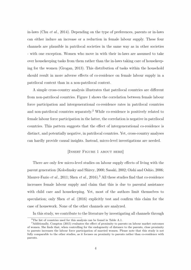


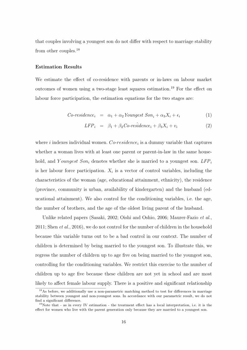


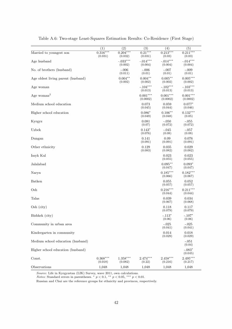


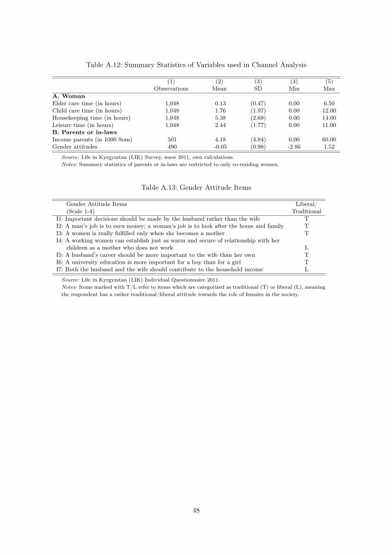


![Fertility Model and Female Labour Force Participation in Selected … · 2013-05-08 · between fertility and female labour force participation [9]. Most studies on labour force participation](https://static.documents.pub/doc/80x56/5e98a78712fceb60083365ee/fertility-model-and-female-labour-force-participation-in-selected-2013-05-08-between.jpg)
