Pattern Recognition Letters 34 (2013) 1916–1927

Contents lists available at SciVerse ScienceDirect

Pattern Recognition Letters

journal homepage: www.elsevier .com/locate /patrec

On-line anomaly detection and resilience in classifier ensembles

0167-8655/$ - see front matter � 2013 Elsevier B.V. All rights reserved.http://dx.doi.org/10.1016/j.patrec.2013.02.014

⇑ Corresponding author. Tel.: +41 788757348.E-mail address: hesam.sagha@epfl.ch (H. Sagha).

Hesam Sagha ⇑, Hamidreza Bayati, José del R. Millán, Ricardo ChavarriagaDefitech Chair in Non-Invasive Brain–Machine Interface, Center for Neuroprosthetics and Institute of Bioengineering, École Polytechnique Fédérale de Lausanne,1015 Lausanne, Switzerland

a r t i c l e i n f o

Article history:Available online 7 March 2013

Keywords:Anomaly detectionClassifier ensembleDecision fusionHuman activity recognition

a b s t r a c t

Detection of anomalies is a broad field of study, which is applied in different areas such as data monitor-ing, navigation, and pattern recognition. In this paper we propose two measures to detect anomalousbehaviors in an ensemble of classifiers by monitoring their decisions; one based on Mahalanobis distanceand another based on information theory. These approaches are useful when an ensemble of classifiers isused and a decision is made by ordinary classifier fusion methods, while each classifier is devoted tomonitor part of the environment. Upon detection of anomalous classifiers we propose a strategy thatattempts to minimize adverse effects of faulty classifiers by excluding them from the ensemble. Weapplied this method to an artificial dataset and sensor-based human activity datasets, with differentsensor configurations and two types of noise (additive and rotational on inertial sensors). We comparedour method with two other well-known approaches, generalized likelihood ratio (GLR) and One-ClassSupport Vector Machine (OCSVM), which detect anomalies at data/feature level.

We found that our method is comparable with GLR and OCSVM. The advantages of our method com-pared to them is that it avoids monitoring raw data or features and only takes into account the decisionsthat are made by their classifiers, therefore it is independent of sensor modality and nature of anomaly.On the other hand, we found that OCSVM is very sensitive to the chosen parameters and furthermore indifferent types of anomalies it may react differently. In this paper we discuss the application domainswhich benefit from our method.

� 2013 Elsevier B.V. All rights reserved.

1. Introduction

The field of activity recognition has gained an increasing level ofinterest driven by applications in health monitoring and assistance,manufacturing and entertainment. In addition, given the advancesin portable sensing technologies and wireless communicationmany of these systems rely on the fusion of the information from(heterogeneous) sensor networks. In this framework, the detectionof anomalous (e.g. faulty or misbehaving) nodes constitute animportant aspect for the design of robust, resilient systems. Be-sides activity recognition, anomaly detection (AD) is an importantissue in the fields of control systems, navigation, and time seriesanalysis. Generally, an anomalous pattern is one that is not desiredor not expected. Therefore it often decreases the system perfor-mance or generates abnormal behavior in the data stream. It canbe due to sensor failure, signal degradation, environmental fluctu-ations, etc. In most fields, such as health monitoring, a desirablecharacteristic is to process the data stream online and get a real-time anomaly detection to take an appropriate counteraction.

As mentioned above, there is a tendency toward the use oflarge number of sensors and with different sensor modalities tohave more information about the observed environment. In a pat-tern recognition system, there are different levels to fuse sensorinformation; data, feature, or classifier. Generally, the goal of datafusion is to achieve more reliable data. Feature fusion concate-nates different features from all the sensors before classification(Fu et al., 2008). Classifier fusion is applicable when an ensembleof classifiers is used and each classifier is assigned to differentsubset of sensors, and finally, the decision is made by a combina-tion of the classifier decisions (Ruta and Gabrys, 2000). This archi-tecture allows for a decentralized classification system whereeach classifier decides about a separate data stream. Therefore,if a particular stream is faulty or misbehaving we can removethe corresponding channel easily from the fusion in order to con-tinue the classification, keeping the system performance as highas possible. A good example of such systems is human activityrecognition (HAR) with on-body sensors mounted on specificlimbs. A good practice is to devote a distinct classifier to eachof the sensors (Roggen et al., 2011). In these systems, one inevita-ble anomaly is the rotation or sliding of the sensors. If theseanomalies can be detected, it is easier to take an appropriatecounter-action for the misbehaving sensor, without the need of

H. Sagha et al. / Pattern Recognition Letters 34 (2013) 1916–1927 1917

reconfiguring the whole system (Sagha et al., 2011a; Chavarriagaet al., 2011). This desirable characteristic is the core feature ofOpportunistic activity recognition systems where elements in thenetwork may appear, disappear or change during life time(Roggen et al., 2009).

Given a classifier ensemble, the anomaly detection process canbe applied at different levels; raw signal or feature level, or at clas-sifier/fusion level. Hereafter, we call both raw and feature level aslow level and the detection process as Low Level Anomaly Detection(LoLAD), while for the later case we name the process as Fusion Le-vel Anomaly Detection (FuLAD). The former case is the most com-monly applied (Chandola et al., 2009), however, it is often notapplicable as different sensor modalities may be available – requir-ing to design specific AD for each modality – as well as the energyand computational cost in the case of wireless sensor networks.Therefore in this paper we introduce an anomaly detection mech-anism at the level of classifier fusion, based on the consistency ofthe classifier decisions. Applying the method on two human activ-ity datasets, we show that, upon detection of anomalous classifiers,an adaptation strategy such as removing them from the fusionchain, leads to a graceful performance degradation.

The structure of the paper is as follows; the next section sum-marizes related work on anomaly detection and resilience, thenwe describe the proposed method in Section 3. The description ofthe experiments and the results are presented in Sections 4 and5, respectively. Finally, we discuss about the use of the methodand its pros and cons in Section 6, followed by a conclusion.

2. Related work

We can handle anomalies in two manners: through detectionand isolation, or by anomaly resilience and adaptation. In the for-mer case, the goal is to detect whether there is an anomaly inthe data or not (detection) and which part of the system is affected(isolation). While for the latter one, the system is designed to betolerant against anomalies, or to be able to take suitable counterac-tion whenever an anomaly is detected. For example, by changingthe network structure in wireless sensor networks (WSN) or adapt-ing parameters to the new data trend.

2.1. Anomaly detection and isolation

Numerous studies have been undertaken to detect anomalies atthe data level. Chandola et al. (2009) survey methods to detectanomalous patterns in a pool of patterns. These methods (such ascomputing distance to the nearest neighbor or to a cluster center,estimating statistical models on the data, discriminating normaland anomalous patterns using artificial neural networks, or supportvector machines) are used in fault detection in mechanical units(Jakubek and Strasser, 2002), structural damage detection(Brotherton and Johnson, 2001), sensor networks (Ide et al., 2007),etc.

Time series change detection (Basseville and Nikiforov, 1993)has been applied to fraud detection (Bolton et al., 2002), computerintrusion detection (Schonlau et al., 2001) and concept drift (Laneand Brodley, 1998). One of the well-known approaches is CUmula-tive SUM (CUSUM) (Page, 1954) which is particularly used whenthe parameters of the changed signal are known. CUSUM computesthe cumulative sum of the log-likelihood ratio of the observationsand once this value exceeds a threshold (which can be adaptive) itis considered a change. It is widely used in change and drift detec-tion in time series (Wu and Chen, 2006), exerting neuro-fuzzymodels (Xie et al., 2007), auto-regressive models (El Falou et al.,2000), and Kalman filters (Severo and Gama, 2010) to generateresiduals whose changes should be detected. Li et al. proposed a

subspace approach to identify optimal residual models in a multi-variate continuous-time system (Li et al., 2003).

When the parameters of the changed signals are unknown,generalized likelihood ratio (GLR) (Lorden, 1971) and adaptiveCUSUM are proposed. GLR maximizes the likelihood ratio over pos-sible values of the parameter of the changed signal, assuming thenormal data follows a Gaussian distribution. It is widely used forchange detection in brain imaging (Bosc et al., 2003), diffusion ten-sor imaging for monitoring neuro-degenerative diseases (Boisgon-tier et al., 2009), for detecting land mines using multi-spectralimages (Anderson, 2008), and target detection and parameterestimation of MIMO radar (Xu and Li, 2007). In the same class,Adaptive CUSUM is able to detect changes by suggesting a distribu-tion for the unknown change model based on the distribution ofthe known model of unaltered data (Alippi and Roveri, 2006a,b,2008). One-Class Support Vector Machine (OCSVM) is anothercommon approach for anomaly detection (Das et al., 2011). Itsrationale is to compute a hyperplane around train data and sam-ples are considered anomalous if they fall outside that hyperplane.

Other approaches have also been proposed in control systems todetect abnormal sensors. One is to extract the model of the systemand detect faults by monitoring residual error signal (Hwang et al.,2010). Another more complex way is to create the input–outputmodel of the system by regression methods and detect potentialfaults when there is a change in the estimated parameters (Ding,2008; Smyth, 1994).

There are many studies and methods toward detection of faultand changes in the sensor networks. In this area, anomaly detec-tion can be done by having redundancies in the network. Eitherin the form of physical redundancy such as adding extra sensors,thus increasing the cost of the system deployment; or from analyt-ical redundancies (Betta and Pietrosanto, 1998). For instance,Andrieu et al. (2004) discuss particle methods to model validation,change/fault detection, and isolation. In this scope, modelvalidation is a process to ensure reliable operations. A survey onthe approaches to fault detection and isolation in unknown envi-ronments has been done by Gage and Murphy (2010). Chen et al.proposed a probabilistic approach that recognizes faulty sensorsbased on the difference in the measurements of a sensor and itsneighbors (Chen et al., 2006). Other approaches are based on thesimilarity between two time series (Yao et al., 2010), OCSVM(Rajasegarar et al., 2007) and clustering (Rajasegarar et al., 2006)to detect outliers in a sensor network, and kernel-based methods(Camps-Valls et al., 2008) to detect changes in remote imagingsystems.

2.2. Anomaly resilience and adaptation

In sensor networks there are different strategies to introducerobustness against changes and drifts in the sensors. Luo et al.(2006) discuss how to optimize the parameters of the model of asensor under both noisy measurement and sensor fault. In turn,Demirbas (2004) proposes scalable design of local self-healing forlarge-scale sensor network applications, while Koushanfar et al.(2002) propose to use an heterogeneous back-up scheme to substi-tute faulty sensors. Other different designs, principles and servicemanagements have been proposed to provide self-healing servicesand diagnosing the true cause of performance degradation(Krishnamachari and Iyengar, 2003; Ruiz et al., 2004; Sheth et al.,2005).

Alternatively, the system can be adapted to dynamic changes.Snoussi and Richard (2007) model the system dynamics, includingabrupt changes in behavior, and select only a few active nodesbased on a trade-off between error propagation, communicationsconstraints and complementarity of distributed data. Wei et al.(2009) used discrete-state variables to model sensor states and

Fig. 1. Classifier fusion architecture. FuLAD (DB) process is shown in gray.

1918 H. Sagha et al. / Pattern Recognition Letters 34 (2013) 1916–1927

continuous variables to track the change of the system parameters.Alternatively, fault detection in WSN has been addressed by find-ing linear calibration parameters using Kalman and particle filters,and state models (Balzano, 2007). Furthermore, Wang et al. (2005)proposed a fault-tolerant fusion based on error-correction codes inorder to increase the classification performance where each nodesends class labels to the fusion process. Alternatively, Chavarriagaet al. (2011) used mutual information between classifier decisionsto assess the level of noise in an activity recognition scenario.

2.2.1. AD in activity recognition systemsAdvances in sensing, portable computing devices, and wireless

communication has lead to an increase in the number and varietyof sensing enabled devices. Activity recognition systems can fuseinformation from networks of on-body and ambient sensors forbetter performance. In such systems there are several approachesto handle anomalies at the data, feature or classifier level. Someof the mentioned approaches in Section 2.1 could be applicableat the feature level. Another strategy is to identify possible anom-alies and propose a method to compensate for them during thenetwork’s life-time. i.e., for specific well-defined anomalies, adhoc strategies can be devised, but this is application-dependentand may not be easily generalized for other domains. For example,in accelerometer-based HAR, sensor rotations are hardly avoidable.One way to cope is to detect how much rotation is added to the sig-nals, based on a reference, and then rotate the sensor readings backbefore classification (Kunze and Lukowicz, 2008; Steinhoff andSchiele, 2010). An alternative way is to use features or classifiersthat are robust against a particular anomaly. For example, Försteret al. (2009) extract discriminative features based on genetic pro-gramming, which are robust against sensor sliding in body areasensor networks. Another approach is to use an adaptive classifierrobust to specific changes in the feature distribution using anExpectation–Maximization approach (Chavarriaga et al., 2013a).These methods are limited due to the fact that there is a need topre-determine the possible anomalies. Moreover, it may not befeasible to characterize all of them in real world applications andit may be impractical to have a rectifier for all of them.

Depending on the limitations of a sensor network, such as thebandwidth, the power consumption, the modality and the cost ofeach node, in practice it may not be feasible to design an efficientLoLAD for a pattern recognition system as the ones described inthis Section. This process can increase the requirements of compu-tational power and energy consumption of each node, dependingon the sampling rate and/or bandwidth. Also, as mentionedpreviously, designing an AD for each modality may not be feasible.In order to come up with these limitations there is a need to reducethe communication of the nodes and make the AD independent ofthe modality. Aiming at overcoming these limitations, we proposea method for AD at the fusion level, particularly suitable forclassifier ensembles.

Classifier ensembles can provide great flexibility to recognitionsystems. In particular, when an anomalous classifier is detected,the ensemble can be reconfigured so as to reduce performancedegradation. The simplest way would be to remove it from theensemble by turning the node off or forcing it into stand-by mode.Other approaches can attempt to adapt or retrain the anomalousclassifiers with the new data. In this case, since the ground truthlabels are not provided online, we can use the best classifier in theensemble as a trainer (Calatroni et al., 2011). Another way, is toupdate the fusion parameters based on the output of the newclassifiers (Sannen et al., 2010). An alternative approach could beto regenerate the decisions of anomalous classifiers based on thedecisions of the other classifiers and then use the same fusionstructure as before (Sagha et al., 2010). In this work we focus onthe detection of the anomalous classifiers and use the first strategy

(i.e., removal) to assess the increased robustness of the entiresystem.

3. Method

We propose a method to automatically detect anomalies in aclassifier ensemble at the fusion level, as shown in Fig. 1. Theclassifier ensemble architecture is more convenient in the sensornetworks deployed for pattern recognition in the sense that differ-ent modalities could be covered with different classifiers and alsothe ensemble could be easily reconfigured to attain differentcriteria such as cost and accuracy (Chavarriaga et al., 2011).

The rationale behind the method is to find a model of classifiercoherence from the training set. Then, at run time, looking at asequence of classifiers’ outputs, we determine how much eachclassifier deviates from this model. Whenever this deviationexceeds a defined threshold the classifier is considered asanomalous. Finally, to make the system resilient, we remove theanomalous classifiers and reconfigure the ensemble.

To compute the deviation, we present two measures. One isbased on the Mahalanobis distance, Section 3.1, and the other isbased on an information theoretic approach, Section 3.2. Later,we will discuss the pros and cons of each approach. The first wasoriginally proposed by Sagha et al. (2011b) and here we providefurther characterization of it. Moreover, in order to compare theperformance of the fusion level and feature level methods, inSections 3.3 and 3.4 we describe two commonly used anomalydetection methods: GLR and OCSVM.

3.1. Distance based detection (DB)

We assume that a given classifier s in the ensemble and thefused output yield posterior probability vectors, os ¼ ½p1; p2; . . . ;

pC � and f ¼ ½p1; p2; . . . ; pC � respectively, where each element de-notes the probability of the sample belonging to a specific classc 2 ½1; . . . ;C�. Fig. 1 shows the process of detection. By calculatingthe distance between each classifier output and the final fusionoutput we can deduce how similar they are. At runtime, if the aver-age distance over the last w decisions exceeds a pre-definedthreshold, the corresponding classifier will be marked as anoma-lous, while other classifiers are considered healthy.

The computed distance should take into account the informa-tion obtained from the training set. We propose the Mahalanobisdistance, Dsc , which stores information about the classifier coher-ence and correlation in a covariance matrix. The average distanceover past w decisions, ~Dsc , is defined as

~Dsc0 ðt0Þ ¼1w

Xt0

t¼t0�w

ðost � ftÞTU�1sc0 ðost � ftÞ; ð1Þ

where ost is the output of the classifier s 2 ½1; . . . ;N� and ft is thefusion output at time t. c0 2 ½1; . . . ;C� is the recognized class after

H. Sagha et al. / Pattern Recognition Letters 34 (2013) 1916–1927 1919

classifier fusion. Usc0 represents the covariance between theclassifier s and the fusion output, for class c0. The covariance matrixis estimated based on the training data set,

Usc ¼ Eððocs � f cÞTðoc

s � f cÞÞ; ð2Þ

where ocs and f c are the output of the classifier s and the output of

the fusion for the specific class c 2 ½1; . . . ;C�, respectively, and Eð�Þis the mathematical expectation. When the distance between aclassifier and fused output is larger than the correspondingthreshold for the chosen class, we label the classifier as anomalous.Thresholds, Hsc , are set individually for each classifier and classsuch that

Hsc ¼ kmaxðDtrscÞ; ð3Þ

where maxðDtrscÞ is the maximum distance for class c and classifier s

computed on the training set. The constant k > 0 is the same for allthe classes and classifiers, and denotes the sensitivity of the detec-tion. Larger values of k result in less sensitive detection. In thiswork, we use the max function which is simple yet reasonable,although more complex threshold estimations could also be applied(e.g. by assessing the distance distribution).

Once one classifier is labeled as anomalous, we exclude it fromthe fusion process. As a result the final fusion decision may change.Therefore, to detect all the anomalous parts we perform the detec-tion process iteratively until the distances of the remaining classi-fiers are below the threshold or a predefined minimum number ofhealthy classifiers, nHmin, is reached.

Moreover, we add a fixed epsilon value (0.01) to the diagonalelements of the covariance matrix to avoid singularities, and anupper bound is used to avoid large Mahalanobis distance values,which affect the anomaly recognition. The bound is set for all clas-ses and classifiers using training data and is obtained as a scaledfactor of the maximum value of Dtr

sc . So

Dsc ¼Dsc Dsc < CmaxðDtr

scÞCmaxðDtr

scÞ Dsc P CmaxðDtrscÞ

(ð4Þ

The final algorithm is as follows:

beginUsc � Covariance matrix for classifier s and class cHsc � Distance threshold for classifier s and class cnHealthy � Number of healthy detected classifiers (init. = N)nHmin � minimum number of classifiers for fusion~Dsc � Average distance over specified windowf ðSÞ � Fusion of classifiers in set SH � set of healthy sensors (initially H ¼ ½s1::sn�)faulty � set of anomalous classifiers (init. ¼ /)while nHealthy > nHmin

f ¼ fusionðHÞc0 ¼ argmaxcðf ÞCompute distance ~Dsc0 8s 2 Hif maxð~Dsc0 Þ < Hsc

exitelsefaulty = [faulty argmaxsð~Dsc0 Þ�nHealthy = nHealthy � 1

endend

3.1.1. Computational costThis procedure iterates at most N � nHmin times for computing

distances, where N is the number of classifiers and nHmin is theminimum number of classifiers for fusion. At each iterationnHealthy distances between each classifier and the fusion outputare computed. The cost of calculating each distance is two vector

subtractions of size C (number of classes) and a multiplication ofthree matrices of sizes 1� C; C � C, and C � 1. Finally the orderof computation is OðN2C3Þ.

3.2. Information Theoretic approach (IT)

Information theory is a wide spread domain which has beenused for signal processing, cryptography, feature selection, amongothers (Shannon, 2001). Two key concepts in information theoryare the entropy, which denotes the amount of information of a ran-dom variable, and the mutual information, which quantifies theshared information between two random variables. The entropyof a random variable X is obtained by

HðXÞ ¼ �X

i

pðxiÞlog2pðxiÞ; ð5Þ

where xi are possible values of X. Mutual information (MI) betweenrandom variables X and Y is defined by

MIðX; YÞ ¼Xx;y

pðx; yÞlog2pðx; yÞ

pðxÞpðyÞ ; ð6Þ

where pðx; yÞ is the joint probability.In the case of an anomalous classifier, we expect its mutual

information with the rest of the classifiers to change (Chavarriagaet al., 2011). In consequence, MI changes between the classifierscould be used to detect anomalies in the ensemble.

To identify which part of the system is anomalous, some careshould be taken when using these values; In order to have an on-line detection, the computation of MI on the test set, MItest, is donein a sliding window of classifier decisions. Inside the window, thedistribution of ground truth labels may vary compared to the train-ing set (e.g. always feeding data from one class would result inentropies and MI values equal to zero). This variation causes a com-mon change in the estimation of MI elements. We call it commoninformation change (CIC) which is measured in bits and computedas the minimum difference value between pairwise elements ofMItest and the one on training set, MItrain. To remove this effect,we remove this difference from the computed MI. The algorithmis as follows:

beginfaulty � set of faulty detected classifiers (init. ¼ /)nHealty � Number of healthy detected classifiers, (init. ¼ N)dif = MItrain � MItest

CIC = min(dif)sub = dif � CICsubii ¼ 0; % removing entropywhile true

si ¼P

jR faulty subij

if max(s) > nHealhty � kfaulty = [faulty argmax(s)]nHealthy = nHealthy � 1elsebreak

endif nHealhty = nHmin

breakend

end

Again, k denotes the sensitivity, dif is the difference between MIof training and testing and its minimum value corresponds to theCIC. Afterwards, we set the diagonal values of the consequent ma-trix to zero to remove the entropy. Finally, the loop starts detectinganomalous classifiers until no value exceeds the threshold.

Table 1Sensor configurations. The number of classifiers for each configuration is written inparenthesis for car manufacturing dataset and opportunity dataset, respectively.

Mode Acc Acc + Gyro Acc + Gyro + Magnetic

L Configl1ð7;5Þ Configl2ð7;5Þ Configl3ð7;5ÞS – Configs2ð14;10Þ Configs3ð21;15Þ

1920 H. Sagha et al. / Pattern Recognition Letters 34 (2013) 1916–1927

Opposite to the previous measure, this approach does not re-quire the classifiers/fusion to provide their outputs as a probabilityvector. The decision of the classifiers can be discrete or nominalvalue.

3.2.1. Computational costThe calculation requires the estimation of MI in a window of

length w; OðwC2N2Þ, then we have a matrix subtraction OðN2Þand the iteration continues at most until we reach to the nHmin.So finally the computation order is OðwC2N2 þ N3Þ.

3.3. Generalized Likelihood Ratio (GLR)

As a comparison we used two standard approaches that detectsanomalies at the feature level. The first approach is based on Gen-eralized Likelihood Ratio for vector based problems where the ini-tial distribution of data h0 is known but it is unknown after change,

HðtÞ ¼¼ h0; when t < t0;

– h0; when t P t0;

�ð7Þ

where t0 is the time when change happens. The GLR solution leadsto the following equation (Basseville and Nikiforov, 1993):

gt ¼ maxt�w6j6t

t � jþ 12

ð�Ytj � h0ÞTR�1ð�Yt

j � h0Þ; ð8Þ

where �Ytj is the mean of the data vector from time j to time t. We

mark the data as anomalous when gt is greater than a threshold.Here, we set the threshold as the maximum value of gt on thetraining set.

3.4. One-Class Support Vector Machine (OCSVM)

One-Class Support Vector Machine computes a hyperplanearound the training data, every test data point outside this hyper-plane is considered as anomalous. Two parameters must be tunedfor this method; m, which is the upper bound of the fraction of thetraining data that are considered to be outside the hyperlane andbandwidth, r, which affects the smoothness of decision boundary.To set these parameters, different optimization approaches areproposed (Zhuang and Dai, 2006; Lukashevich et al., 2009). Here,we experimentally set the best parameters so as to have a gooddetection accuracy on the rotational noise, Section 4.2.4. We haveused LIBSVM implementation (Chang and Lin, 2011).

1 For the complete list of the labels please refer to Stiefmeier et al. (2008).2 <http://archive.ics.uci.edu/ml/datasets/OPPORTUNITY+Activity+Recognition>.3 Ubisense: <http://www.ubisense.net/>.

4. Experiments

The performance of the proposed methods has been evaluatedon one artificially generated dataset and two real datasets of hu-man activities. The activity datasets contain several sensor modal-ities, and different ensemble configurations were tested based onthe sensor modalities or location.

4.1. Synthetic dataset

The synthetic dataset consists of different classifier ensembleswhere we systematically test different sizes, accuracies and levelsof noise. The number of classifiers and classes ranges from 2 to 16and 3 to 15 with the step of 2 and 3, respectively. The number ofsamples per class was set to 60 for both the training and the testingsets and they are randomly distributed over time. In each simula-tion, the accuracy of the healthy classifiers was set to 80%, whilethe performance of anomalous classifiers ranges from 10% to70%. The number of anomalous classifiers varies from 0% to 100%of the available classifiers for each experiment. These values pro-

vide a general assessment on the methods and the effect of noisefor different ensemble configurations and number of classes.

In each experiment, we change one of the following character-istics: number of classes, number of classifiers, percentage ofanomalous classifiers, or the level of anomaly. Presented resultsare the average across 5 repetitions per each experiment.

4.2. Human activity datasets

4.2.1. DatasetsThe two real datasets contain data from body mounted inertial

sensors, recorded while human subjects perform different activi-ties. In order to emulate changes in the sensor network we artifi-cially added different levels of noise to the sensor readings andassessed the method ability to detect noisy channels, as well asthe recognition performance.

The first dataset corresponds to a car manufacturing scenario(Stiefmeier et al., 2008). It contains data from 8 subjects perform-ing 10 recording sessions each (except one subject who recordedonly 8 sessions). The sensors are accelerometers, rate gyros, andmagnetic sensors mounted on different parts of the body (i.e.,hands, upper and lower arms, and chest). There are 20 activity clas-ses to be recognized, such as Open/Close hood, Open/Check/Closetrunk.1 We use leave-one-subject-out cross validation for evaluatingthe performance, and the classes are segmented and randomlydistributed.

The second dataset, named Opportunity dataset, comprises sen-sory data of different modalities in a breakfast scenario. The data-base is fully described by Chavarriaga et al. (2013b) and is publiclyavailable as a benchmark for HAR methods.2 The dataset was re-corded in an instrumented kitchen with two doors and a dining tableat the center. The different sensor modalities are camera, micro-phone, localization,3 reed switch, and inertial sensors. Inertial andlocalization sensors are all mounted on a jacket worn by the subjectduring the recording. For the current simulations we use a subset ofthis dataset including 4 subjects and motion jacket inertial sensors.Seventeen activities are detected, such as Open/Close door, Open/Close drawer. For this dataset we also evaluate the methods with aleave-one-subject-out cross validation and the data are previouslysegmented and randomly distributed.

4.2.2. ConfigurationsWe tested different sensor configurations using one, two or

three modalities for both datasets (i.e., accelerometer, gyro andmagnetic sensors). The configurations are listed in Table 1. Forone group of them, denoted as configl for location based, each clas-sifier uses data from a set of sensors placed at the same location.For the other group, denoted as configs for sensor type based, weused one classifier per sensor per location (e.g. one classifier forthe tri-axial accelerometer located on the right upper arm). Foreach case the number of classifiers are also provided in the table.

H. Sagha et al. / Pattern Recognition Letters 34 (2013) 1916–1927 1921

4.2.3. ClassificationFor classification we used Quadratic Discriminant Analysis

(QDA), unless otherwise stated. As features we used the meanand variance of the segmented signals. For each class (i.e., activity),the covariance matrix has been estimated, which is constrained tobe diagonal due to the lack of sufficient data to estimate the fullcovariance matrix. The decisions of individual classifiers are fusedusing a naïve Bayesian approach. It uses the normalized confusionmatrix of each classifier to represent the total reliability of thisclassifier for each class. The fused output can be computed asfollows:

Cout ¼ arg maxa

Ys

PðC ¼ cijOs ¼ osÞ !

; os 2 c1; . . . ; cm; ð9Þ

where Os is the class label from the classifier s. Computing the prob-abilities is straightforward using Bayes rule:

0102030405060

0 1 2 3 4 5 6

0

0.5

1

noise level (deg)# of noisy sensors

Accu

racy

02

46

810

0 1 2 3 4 5 6

0

0.5

1

noise level (SNR)# of noisy sensors

Accu

racy

0102030405060

01

23

4

0

0.2

0.4

0.6

noise level (deg)# of noisy sensors

Accu

racy

0246810

01

23

4

0

0.2

0.4

0.6

noise level (SNR)# of noisy sensors

Accu

racy

Fig. 2. The effect of noise on the overall classification accuracy after fusion. HARdatasets – Configl2. Left: rotational noise, the level is in degree. Right: additive noise,the level is in SNR.

0.1 0.2 0.3 0.4 0.5 0.6 0.7

1020304050607080900

0.5

1

1.5

Accuracy of faulty classifiers

% of faulty classifiers

Mea

n of

dis

tanc

e

Mean FaultyMean Healthy

Accuracy of faulty classifiers

% o

f fau

lty c

lass

ifier

s

0.1 0.2 0.3 0.4 0.5 0.6 0.7

0.1

0.2

0.3

0.4

0.5

0.6

0.7

0.8

0.9 0.1

0.2

0.3

0.4

0.5

0.6

0.7

0.8

0.1 0.2 0.3 0.4 0.5 0.6 0.7

1020304050607080900

5

10

15

20

Accuracy of faulty classifiers

% of faulty classifiers

Mea

n of

dis

tanc

e

Mean FaultyMean Healthy

Accuracy of faulty classifiers

% o

f fau

lty c

lass

ifier

s

0.1 0.2 0.3 0.4 0.5 0.6 0.7

0.1

0.2

0.3

0.4

0.5

0.6

0.7

0.8

0.9 2

4

6

8

10

12

14

(a) DB-noiseassessment

(c) IT-noiseassessment

Fig. 3. Synthetic dataset. Left: the effect of (a) and (c) noise and ratio of noisy sensors, (b)faulty and healthy. Each plot shows the average distance computed for faulty and healthycolour in this figure legend, the reader is referred to the web version of this article.)

PðC ¼ cijOs ¼ osÞ / PðCÞPðOs ¼ osjC ¼ ciÞ: ð10Þ

We suppose that the priors PðCÞ of all the classes are the same, andPðOs ¼ osjC ¼ ciÞ is the confusion matrix estimated on the trainingdata.

In addition, to show the generality of the approach we also per-form simulations using other classification and fusion methods(Linear driscriminant analysis and Dempster–Shafer fusion).

4.2.4. Simulated anomaliesWe simulate anomalies by introducing rotational and additive

noise to the testing signals. Each type of noise was tested sepa-rately in the three datasets for different configurations (i.e., num-ber of faulty classifiers, level of noise). In each simulation, noiseis added to a fixed number of randomly chosen sensors for the en-tire test set. We report results on 10 repetitions of eachconfiguration.

In the case of rotational noise, for each simulation the levelnoise is randomly chosen between 0� and 60� (with intervals of10�). For additive noise the levels correspond to Signal to Noise Ra-tios of 0 to 10 dB with a step of 2 dB. As a reference, Fig. 2 showshow the classification performance in the HAR datasets degradeswith the increase of the noise level and the amount of faultyclassifiers.

5. Results

5.1. Synthetic dataset

Fig. 3 illustrates the effect of the number of faulty classifiers andtheir accuracies for the synthetic dataset. It shows the averagecomputed distances (over the number of classes and classifiers)for the healthy and faulty classifiers (Mean Healthy and MeanFaulty, respectively) for the two proposed measures; Mahalanobisdistance and mutual information. The results suggest that the ITmeasure performs better than DB when the number of noisy sen-sors and noise itself are higher. That is because a large number offaulty sensors will affect the fusion output, thus affecting thedetection using the DB approach. In contrast, the IT approach only

2 4 6 8 10 12 14 16 3 6

9 12

150

0.5

1

# of classifiers# of classes

Mea

n of

dis

tanc

e

Mean FaultyMean Healthy

# of classes

# of

cla

ssifi

ers

2 4 6 8 10 12 14 16

3

6

9

12

150.2

0.3

0.4

0.5

0.6

2 4 6 8 10 12 14 16 3 6

9 12

150

5

10

15

20

# of classifiers# of classes

Mea

n of

dis

tanc

e

Mean FaultyMean Healthy

# of classes

# of

cla

ssifi

ers

2 4 6 8 10 12 14 16

3

6

9

12

152

4

6

8

10

12

(b) DB-classificationassessment

(d) IT-classificationassessment

and (d) number of classes and classifiers on the distance. Right: difference betweenclassifiers (red and blue traces respectively). (For interpretation of the references to

1922 H. Sagha et al. / Pattern Recognition Letters 34 (2013) 1916–1927

considers the relation between classifiers without considering thefused output.

In contrast, as it is shown in Fig. 3(b) and (d) when there are fewclassifiers or classes, DB is able to detect the anomalies better. Ingeneral, the number of classes has more effect on DB, while thenumber of classifiers has more effect on the IT-based measure.

5.2. Human activity datasets

Besides comparison with the LoLAD approach (i.e., GLR andOCSVM methods), we also compare the proposed methods with areference performance corresponding to a ‘perfect removal’ ap-proach. In this case we exclude from the ensemble those classifierswhose decisions are affected by the noise. This yields an upperbound on the performance that can be achieved based on the re-moval of anomalous classifiers. Obviously, such a removal cannot

0 1 2 3 4 5 60.2

0.3

0.4

0.5

0.6

0.7

0.8

# of noisy sensors

Cla

ssifi

catio

n ac

cura

cy

0 1 2 30.4

0.5

0.6

0.7

0.8

0.9

1

# of noisy sens

Cla

ssifi

catio

n ac

cura

cy

1 3 5 7 9 11 130.4

0.5

0.6

0.7

0.8

0.9

1

# of noisy sensors

Cla

ssifi

catio

n ac

cura

cy

0

0

0

0

0

0

Cla

ssifi

catio

n ac

cura

cy

0 1 2 3 4 5 60.2

0.3

0.4

0.5

0.6

0.7

# of noisy sensors

Cla

ssifi

catio

n ac

cura

cy

0 1 2 30.1

0.2

0.3

0.4

0.5

0.6

0.7

0.8

0.9

# of noisy sens

Cla

ssifi

catio

n ac

cura

cy

1 3 5 7 9 11 130.6

0.65

0.7

0.75

0.8

0.85

0.9

0.95

1

# of noisy sensors

Cla

ssifi

catio

n ac

cura

cy

0

0

0

0

Cla

ssifi

catio

n ac

cura

cy

Fig. 4. Classification accuracy before and after anomaly detection. Car manufacturing datscale on y-axis.

be performed at run-time since there is no information aboutnoise. For all simulations we set k ¼ 1, window length = 50, andin the case of DB measure, C ¼ 5.

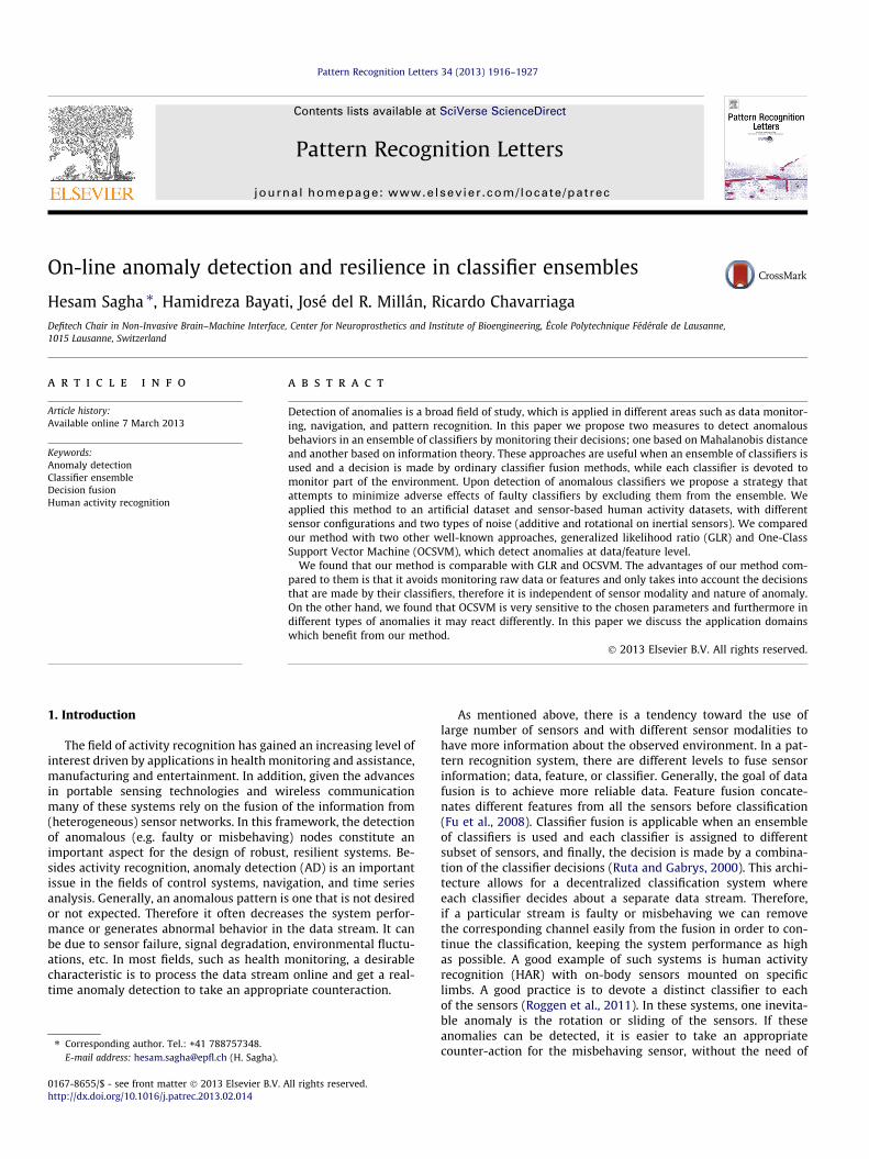
The classification accuracies for the car manufacturing datasetare shown in Fig. 4 with different sensor configurations for rota-tional and additive noise, respectively. Similarly, Fig. 5 presentsthe results on the Opportunity dataset. Given the characteristicsof the latter dataset, i.e., larger number and variety of realisticactivities, the classification accuracy is lower (e.g. below 70% withQDA) than in the car manufacturing dataset.

Obviously, when no action is taken the performance decreasesdramatically in both datasets (c.f. Fig. 2; green traces in Figs. 4and 5). In general, GLR performs satisfactorily in all situations, aswell as the IT-based method. Although for the latter, the perfor-mance decreases dramatically when there are less than threehealthy classifiers in the Location-based configurations (configl�).This is certainly due to the low number of available classifiers.

4 5 6ors

0 1 2 3 4 5 60.4

0.5

0.6

0.7

0.8

0.9

1

# of noisy sensorsC

lass

ifica

tion

accu

racy

4 9 14 19.4

.5

.6

.7

.8

.9

1

# of noisy sensors

4 5 6

ors

0 1 2 3 4 5 60.1

0.2

0.3

0.4

0.5

0.6

0.7

0.8

0.9

# of noisy sensors

Cla

ssifi

catio

n ac

cura

cy

4 9 14 190.6

.65

0.7

.75

0.8

.85

0.9

.95

1

# of noisy sensors

aset, (a)–(e) Rotational noise, (f)–(j) Additive noise. Note: (a) and (f) have a different

0 1 2 3 40.2

0.25

0.3

0.35

0.4

0.45

0.5

# of noisy sensors

Cla

ssifi

catio

n ac

cura

cy

0 1 2 3 40.2

0.3

0.4

0.5

0.6

0.7

# of noisy sensors

Cla

ssifi

catio

n ac

cura

cy

0 1 2 3 40.2

0.3

0.4

0.5

0.6

0.7

# of noisy sensors

Cla

ssifi

catio

n ac

cura

cy

1 3 5 7 90.2

0.3

0.4

0.5

0.6

0.7

# of noisy sensors

Cla

ssifi

catio

n ac

cura

cy

1 3 5 7 9 11 130.2

0.3

0.4

0.5

0.6

0.7

# of noisy sensors

Cla

ssifi

catio

n ac

cura

cy

0 1 2 3 40

0.1

0.2

0.3

0.4

0.5

# of noisy sensors

Cla

ssifi

catio

n ac

cura

cy

0 1 2 3 40.1

0.2

0.3

0.4

0.5

0.6

0.7

# of noisy sensors

Cla

ssifi

catio

n ac

cura

cy

0 1 2 3 40.1

0.2

0.3

0.4

0.5

0.6

0.7

# of noisy sensors

Cla

ssifi

catio

n ac

cura

cy

1 3 5 7 90.1

0.2

0.3

0.4

0.5

0.6

0.7

# of noisy sensors

Cla

ssifi

catio

n ac

cura

cy

1 3 5 7 9 11 130.1

0.2

0.3

0.4

0.5

0.6

0.7

# of noisy sensors

Cla

ssifi

catio

n ac

cura

cy

Fig. 5. Classification accuracy before and after anomaly detection. Opportunity dataset, (a)–(e) Rotational noise, (f)–(j) Additive noise. Note: (a) and (f) has a different scale ony-axis.

H. Sagha et al. / Pattern Recognition Letters 34 (2013) 1916–1927 1923

The performance of the DB measure is similar when less than halfof the sensors are faulty. In turn, OCSVM reacts close to GLR for thecar manufacturing dataset, but performs poorly on the seconddataset. This results from its sensitivity to the number of features,and data distribution, highlighting the need for tuning the param-eters for each configuration (we kept the parameters which wastuned for configl2 for all other configurations).

Altogether, the results show that (a) both LoLAD and FuLADsucceed in increasing the classification accuracy, (b) There is apossibility of detecting anomalies at fusion level, with comparableperformance to LoLAD.

As an example, Fig. 6 shows the average detection accuracyacross subjects with respect to the level of noise, for LoLAD andFuLAD in the car manufacturing dataset using Configl2 . It iscomputed as:

DetectionAccuracy ¼ TruePositive þ TrueNegative#of samples � #of sensors

; ð11Þ

where TruePositive is the correctly detected noisy sensors andTrueNegative is the correctly detected unaffected sensors and # ofsamples is the number of samples in the trial. They show that oncethe level of noise is low, the anomaly spotting is poor while byincreasing the level of noise, it rises. This is due to the fact that theselevels of noise do not affect the classifier decisions. Hence, theinability to spot them does not impact the overall system perfor-mance, see Fig. 2.

Fig. 7(a) and (c) show the average number of required iterationsper pattern with respect to the number of noisy sensors and thelevel of rotational noise for both methods. During the DB iterationsas anomalous classifiers are removed from the ensemble, the

0 10 20 30 40 50 600

0.2

0.4

0.6

0.8

1

0

Noise level

Det

ectio

n ac

cura

cy

123456

0 10 20 30 40 50 600

0.2

0.4

0.6

0.8

1

0

Noise levelD

etec

tion

accu

racy

1234

(a) GLR

0 10 20 30 40 50 600

0.2

0.4

0.6

0.8

1

Noise level

Det

ectio

n ac

cura

cy

0123456

0 10 20 30 40 50 600

0.2

0.4

0.6

0.8

1

Noise level

Det

ectio

n ac

cura

cy

01234

(b) OCSVM

0 10 20 30 40 50 600

0.2

0.4

0.6

0.8

1

0

Noise level

Det

ectio

n ac

cura

cy

123456

0 10 20 30 40 50 600

0.2

0.4

0.6

0.8

1

0

Noise level

Det

ectio

n ac

cura

cy

1234

(c) DB

0 10 20 30 40 50 600.1

0.2

0.3

0.4

0.5

0.6

0.7

0.8

0.9

01

Noise level

Det

ectio

n ac

cura

cy

23456

0 10 20 30 40 50 600

0.2

0.4

0.6

0.8

1

0

Noise level

Det

ectio

n ac

cura

cy

1234

(d) IT

Fig. 6. Anomaly detection accuracy. Left: car manufacturing dataset, Right:opportunity dataset. Configl2, rotational noise. Each curve corresponds to a differentnumber of noisy sensors.

Noise level

# of

noi

sy s

enso

rs

0 10 20 30 40 50 60

0

1

2

3

4

5

6 1.5

2

2.5

3

3.5

4

4.5

5

5.5

Noise level

# of

noi

sy s

enso

rs

0 10 20

0

1

2

3

4 1.2

1.4

1.6

1.8

2

2.2

2.4

2.6

2.8

(a) Averagenumberofiterations(DB)

Noise level

# of

noi

sy s

enso

rs

0 10 20 30 40 50 60

0

1

2

3

4

5

60

0.2

0.4

0.6

0.8

1

1.2

1.4

1.6

1.8

Noise level

# of

noi

sy s

enso

rs

0 10 20

0

1

2

3

40.1

0.2

0.3

0.4

0.5

0.6

(b) Numberofchangeddecisions(DB)

Noise level

# of

noi

sy s

enso

rs

0 10 20 30 40 50 60

0

1

2

3

4

5

60

0.2

0.4

0.6

0.8

1

1.2

1.4

1.6

1.8

Noise level

# of

noi

sy s

enso

rs

0 10 20

0

1

2

3

41.2

1.4

1.6

1.8

2

2.2

2.4

(c) Averagenumberofiterations(IT)

Fig. 7. The average number of iterations and changing decisions. Left: carmanufacturing dataset, Right: opportunity dataset. Configl2, rotational noise.

1924 H. Sagha et al. / Pattern Recognition Letters 34 (2013) 1916–1927

fusion output may change its decision; the average number ofchanges is shown in Fig. 7(b). Unsurprisingly, as the noise or thenumber of noisy sensors increases, the number of loops andchanges of decisions also increases as more classifiers arerecognized as anomalous.

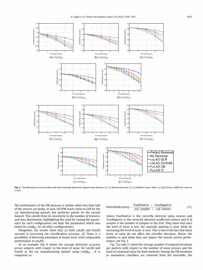
The effect of the window length for DB and IT on the accuracy ofdetection (car manufacturing database) is shown in Fig. 8(a) and(b), respectively. Results show that a window length of 50 samplesyields the best results. Of course, there is a trade-off of choosingthe window length: lower values may lessen the performancewhile larger values impose a delay on the detection.

Fig. 8(c) and (d) illustrates how the threshold value affects theanomaly detection and classification accuracy, for DB method. Itshows that a threshold value equal to one yields good resultsand it is reasonable since only distances in the range of the trainingdataset are permitted. Also, we empirically found that for this

dataset, setting the value of C at least twice the threshold valueand at most three times the threshold achieves the best results.

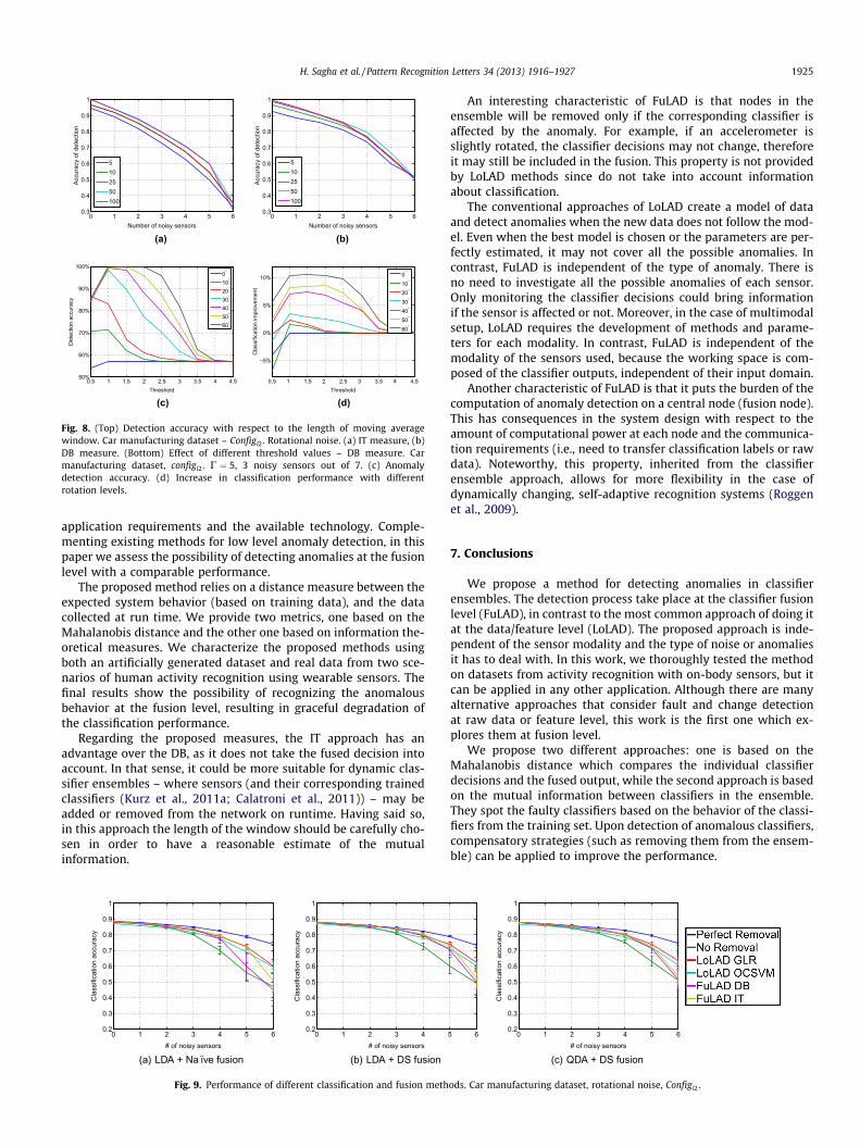
To demonstrate that the methods do not depend on the classi-fication or fusion method we tested them when a Linear Discrim-inative Classifier (LDA) is used, as well as when Dempster–Shaferfusion (Kuncheva et al., 2001) is applied for combining the classifi-ers. Fig. 9 shows the results obtained on the car manufacturingdataset with rotational noise. It is obvious that the IT approach isnot dependent on the fusion method, since it is not using its out-put. But as the results show, the DB approach also is not particu-larly sensitive to the type of classifier or fusion methods.Comparing the performance of QDA (Fig. 4(b)) and LDA(Fig. 9(a)), the former appears more robust to this kind of noise.As expected, Dempster–Shafer fusion (Fig. 9(c)) is also less sensi-tive to noise than the naïve fusion.

6. Discussion

Nowadays, multimodal sensor networks are increasingly usedto gather information about the environment and improve contextand activity recognition. Classifier ensembles can provide an effi-cient and flexible approach to achieve this. However, sensors arealways prone to noise and anomalies that may degrade the systemperformance. Therefore, the ability of detect such anomalies mayallow to dynamically adapt the system, bringing more robustnessto the recognition chain.

Anomaly detection can be performed at the data/feature or fu-sion level. This choice depends on several factors, including the

0 1 2 3 4 5 60.3

0.4

0.5

0.6

0.7

0.8

0.9

1

Number of noisy sensors

Accu

racy

of d

etec

tion

5102550100

(a)

0 1 2 3 4 5 60.3

0.4

0.5

0.6

0.7

0.8

0.9

1

Number of noisy sensors

Accu

racy

of d

etec

tion

5102550100

(b)

0.5 1 1.5 2 2.5 3 3.5 4 4.550%

60%

70%

80%

90%

100%

Threshold

Det

ectio

n ac

cura

cy

0°

10°

20°

30°

40°

50°

60°

(c)

0.5 1 1.5 2 2.5 3 3.5 4 4.5

−5%

0%

5%

10%

Threshold

Cla

ssifi

catio

n im

prov

emen

t

0°

10°

20°

30°

40°

50°

60°

(d)

Fig. 8. (Top) Detection accuracy with respect to the length of moving averagewindow. Car manufacturing dataset – Configl2. Rotational noise. (a) IT measure, (b)DB measure. (Bottom) Effect of different threshold values – DB measure. Carmanufacturing dataset, configl2; C ¼ 5, 3 noisy sensors out of 7. (c) Anomalydetection accuracy. (d) Increase in classification performance with differentrotation levels.

H. Sagha et al. / Pattern Recognition Letters 34 (2013) 1916–1927 1925

application requirements and the available technology. Comple-menting existing methods for low level anomaly detection, in thispaper we assess the possibility of detecting anomalies at the fusionlevel with a comparable performance.

The proposed method relies on a distance measure between theexpected system behavior (based on training data), and the datacollected at run time. We provide two metrics, one based on theMahalanobis distance and the other one based on information the-oretical measures. We characterize the proposed methods usingboth an artificially generated dataset and real data from two sce-narios of human activity recognition using wearable sensors. Thefinal results show the possibility of recognizing the anomalousbehavior at the fusion level, resulting in graceful degradation ofthe classification performance.

Regarding the proposed measures, the IT approach has anadvantage over the DB, as it does not take the fused decision intoaccount. In that sense, it could be more suitable for dynamic clas-sifier ensembles – where sensors (and their corresponding trainedclassifiers (Kurz et al., 2011a; Calatroni et al., 2011)) – may beadded or removed from the network on runtime. Having said so,in this approach the length of the window should be carefully cho-sen in order to have a reasonable estimate of the mutualinformation.

0 1 2 3 4 5 60.2

0.3

0.4

0.5

0.6

0.7

0.8

0.9

1

# of noisy sensors

Cla

ssifi

catio

n ac

cura

cy

(a) LDA + Na ı̈ve fusion

0 1 2 3 40.2

0.3

0.4

0.5

0.6

0.7

0.8

0.9

1

# of noisy sensors

Cla

ssifi

catio

n ac

cura

cy

(b) LDA + DS fusion

Fig. 9. Performance of different classification and fusion meth

An interesting characteristic of FuLAD is that nodes in theensemble will be removed only if the corresponding classifier isaffected by the anomaly. For example, if an accelerometer isslightly rotated, the classifier decisions may not change, thereforeit may still be included in the fusion. This property is not providedby LoLAD methods since do not take into account informationabout classification.

The conventional approaches of LoLAD create a model of dataand detect anomalies when the new data does not follow the mod-el. Even when the best model is chosen or the parameters are per-fectly estimated, it may not cover all the possible anomalies. Incontrast, FuLAD is independent of the type of anomaly. There isno need to investigate all the possible anomalies of each sensor.Only monitoring the classifier decisions could bring informationif the sensor is affected or not. Moreover, in the case of multimodalsetup, LoLAD requires the development of methods and parame-ters for each modality. In contrast, FuLAD is independent of themodality of the sensors used, because the working space is com-posed of the classifier outputs, independent of their input domain.

Another characteristic of FuLAD is that it puts the burden of thecomputation of anomaly detection on a central node (fusion node).This has consequences in the system design with respect to theamount of computational power at each node and the communica-tion requirements (i.e., need to transfer classification labels or rawdata). Noteworthy, this property, inherited from the classifierensemble approach, allows for more flexibility in the case ofdynamically changing, self-adaptive recognition systems (Roggenet al., 2009).

7. Conclusions

We propose a method for detecting anomalies in classifierensembles. The detection process take place at the classifier fusionlevel (FuLAD), in contrast to the most common approach of doing itat the data/feature level (LoLAD). The proposed approach is inde-pendent of the sensor modality and the type of noise or anomaliesit has to deal with. In this work, we thoroughly tested the methodon datasets from activity recognition with on-body sensors, but itcan be applied in any other application. Although there are manyalternative approaches that consider fault and change detectionat raw data or feature level, this work is the first one which ex-plores them at fusion level.

We propose two different approaches: one is based on theMahalanobis distance which compares the individual classifierdecisions and the fused output, while the second approach is basedon the mutual information between classifiers in the ensemble.They spot the faulty classifiers based on the behavior of the classi-fiers from the training set. Upon detection of anomalous classifiers,compensatory strategies (such as removing them from the ensem-ble) can be applied to improve the performance.

5 6 0 1 2 3 4 5 60.2

0.3

0.4

0.5

0.6

0.7

0.8

0.9

1

# of noisy sensors

Cla

ssifi

catio

n ac

cura

cy

(c) QDA + DS fusion

ods. Car manufacturing dataset, rotational noise, Configl2.

1926 H. Sagha et al. / Pattern Recognition Letters 34 (2013) 1916–1927

Besides testing on synthetic data, we applied our method to twoactivity recognition datasets, allowing us to test it in realistic con-ditions using different sensor modalities and configurations. Theresults show the feasibility of change and anomaly detection atthe fusion level and the improvement of the classification for allthe cases. Although the proposed method does not build explicitmodels for each sensor type or modality in the ensemble, its per-formance is comparable to that achieved with LoLAD. The IT mea-sure can detect anomalies just as well as the feature level method,even when only two classifiers remain healthy. Whereas the DBmeasure works satisfactorily until half of the classifiers areaffected.

Alternatively, the distance measures presented here can be usedto quantify the confidence of each classifier in the ensemble at run-time. This measure can then be used to dynamically reconfigurethe ensemble, taking into account different specifications includingclassification performance, as well as communication costs or en-ergy consumption (Kurz et al., 2011b).

Acknowledgments

This work has been supported by the EU Future and EmergingTechnologies (FET) contract number FP7-Opportunity-225938.We would like to thank Sundara Tejaswi Digumarti for his efforton preparing the datasets, and a special thank to Dr. Daniel Roggen,for his useful comments.

References

Alippi, C., Roveri, M., 2006a. An adaptive cusum-based test for signal changedetection. In: IEEE Internat. Symposium on Circuits and Systems (ISCAS). IEEE.

Alippi, C., Roveri, M., 2006b. A computational intelligence-based criterion to detectnon-stationarity trends. In: Internat. Joint Conf. on Neural Networks (IJCNN), pp.5040–5044.

Alippi, C., Roveri, M., 2008. Just-in-time adaptive classifiers. Part I: Detectingnonstationary changes. IEEE Trans. Neural Networks 19, 1145–1153.

Anderson, J., 2008. A generalized likelihood ratio test for detecting land mines usingmultispectral images. IEEE Geosci. Remote Sens. Lett. 5, 547–551.

Andrieu, C., Doucet, A., Singh, S.S., Tadic, V.B., 2004. Particle methods for changedetection, system identification, and control. Proc. IEEE 92, 423–438.

Balzano, L.K., 2007. Addressing fault and calibration in wireless sensor networks.Master’s Thesis, University of California Los Angeles.

Basseville, M., Nikiforov, I.V., 1993. Detection of Abrupt Changes: Theory andApplication. Prentice-Hall.

Betta, G., Pietrosanto, A., 1998. Instrument fault detection and isolation: state of theart and new research trends. In: IEEE Conference Proceedings Instrumentationand Measurement Technology Conference, pp. 483–489.

Boisgontier, H., Noblet, V., Heitz, F., Rumbach, L., Armspach, J.P., 2009. Generalizedlikelihood ratio tests for change detection in diffusion tensor images. In: IEEEInternational Symposium on Biomedical Imaging: From Nano to Macro, pp.811–814.

Bolton, R.J., Hand, D.J., H, D.J., 2002. Statistical fraud detection: A review. Statist. Sci.17, 235–255.

Bosc, M., Heitz, F., Armspach, J.P., Namer, I., Gounot, D., Rumbach, L., 2003.Automatic change detection in multimodal serial MRI: Application to multiplesclerosis lesion evolution. NeuroImage 20, 643–656.

Brotherton, T., Johnson, T., 2001. Anomaly detection for advanced military aircraftusing neural networks. In: IEEE Proceedings of Aerospace Conference, pp. 3113–3123.

Calatroni, A., Roggen, D., Tröster, G., 2011. Automatic transfer of activity recognitioncapabilities between body-worn motion sensors: Training newcomers torecognize locomotion. In: 8th Internat. Conf. on Networked Sensing Systems(INSS), Penghu, Taiwan.

Camps-Valls, G., Gomez-Chova, L., Munoz-Mari, J., Rojo-Alvarez, J., Martinez-Ramon,M., 2008. Kernel-based framework for multitemporal and multisource remotesensing data classification and change detection. IEEE Transactions onGeoscience and Remote Sensing 46, 1822–1835.

Chandola, V., Banerjee, A., Kumar, V., 2009. Anomaly detection: A survey. ACMComput. Surv. 41, 1–58.

Chang, C.C., Lin, C.J., 2011. LIBSVM: A library for support vector machines. ACMTrans. Intell. Syst. Technol. 2, 27:1–27:27, Software available at: <http://www.csie.ntu.edu.tw/cjlin/libsvm>.

Chavarriaga, R., Sagha, H., Millán, J.d.R., 2011. Ensemble creation andreconfiguration for activity recognition: An information theoretic approach.In: IEEE Internat. Conf. on Systems, Man, and Cybernetics.

Chavarriaga, R., Bayati, H., Millán, J.d.R., 2013a. Unsupervised adaptation foracceleration-based activity recognition: robustness to sensor displacementand rotation. Pers. Ubiquitous Comput. 17, 479–490.

Chavarriaga, R., Sagha, H., Calatroni, A., Digumarti, S.T., Tröster, G., Millán, J.d.R.,Roggen, D., 2013b. The opportunity challenge: A benchmark database for on-body sensor-based activity recognition. Pattern Recognition Lett. this issue.

Chen, J., Kher, S., Somani, A., 2006. Distributed fault detection of wireless sensornetworks. In: Proc. Workshop on Dependability Issues in Wireless ad HocNetworks and Sensor Networks. ACM, New York, NY, USA, pp. 65–72.

Das, K., Bhaduri, K., Votava, P., 2011. Distributed anomaly detection using 1-classSVM for vertically partitioned data. Statist. Anal. Data Min. 4, 393–406.

Demirbas, M., 2004. Scalable design for fault-tolerance for wireless sensornetworks. Ph.D. Thesis, Ohio State University, Computer and InformationScience.

Ding, S., 2008. Model-Based Fault Diagnosis Techniques. Springer.El Falou, W., Khalil, M., Duchene, J., 2000. AR-based method for change detection

using dynamic cumulative sum. In: 7th IEEE Internat. Conf. on Electronics,Circuits and Systems, ICECS, vol.1, pp. 157–160.

Förster, K., Brem, P., Roggen, D., Tröster, G., 2009. Evolving discriminative featuresrobust to sensor displacement for activity recognition in body area sensornetworks. In: 5th Internat. Conf. on Intelligent Sensors, Sensor Networks andInformation Processing (ISSNIP), pp. 43–48.

Fu, Y., Cao, L., Guo, G., Huang, T.S., 2008. Multiple feature fusion by subspacelearning. In: Proc. Internat. Conf. on Content-Based Image and Video Retrieval.ACM, New York, NY, USA, pp. 127–134.

Gage, J., Murphy, R.R., 2010. Sensing assessment in unknown environments: Asurvey. IEEE Trans. Syst. Man Cybernet. Part A: Syst. Humans 40, 1–12.

Hwang, I., Kim, S., Kim, Y., Seah, C.E., 2010. A survey of fault detection,isolation, and reconfiguration methods. IEEE Trans. Control Syst. Technol. 18,636–653.

Ide, T., Papadimitriou, S., Vlachos, M., 2007. Computing correlation anomaly scoresusing stochastic nearest neighbors. In: 7th IEEE Internat. Conf. on Data Mining,ICDM, pp. 523–528.

Jakubek, S., Strasser, T., 2002. Fault-diagnosis using neural networks with ellipsoidalbasis functions. In: Proc. American Control Conference, pp. 3846–3851.

Koushanfar, F., Potkonjak, M., Sangiovanni-Vincentelli, A., 2002. On-line faultdetection of sensor measurements. In: IEEE Sensors, pp. 69–85.

Krishnamachari, B., Iyengar, S.S., 2003. Efficient and fault-tolerant feature extractionin wireless sensor networks. In: Proc. 2nd Internat. Workshop on InformationProcessing in Sensor Networks.

Kuncheva, L.I., Bezdek, J.C., Duin, R.P.W., 2001. Decision templates for multipleclassifier fusion: An experimental comparison. Pattern Recognition 34, 299–314.

Kunze, K., Lukowicz, P., 2008. Dealing with sensor displacement in motion-basedonbody activity recognition systems. In: Proc. 10th Internat. Conf. onUbiquitous Computing. ACM, New York, NY, USA, pp. 20–29.

Kurz, M., Hölzl, G., Ferscha, A., Calatroni, A., Roggen, D., Tröster, G., 2011a. Real-timetransfer and evaluation of activity recognition capabilities in an opportunisticsystem. In: 3rd Internat. Conf. on Adaptive and Self-Adaptive Systems andApplications, pp. 73–78.

Kurz, M., Hölzl, G., Ferscha, A., Sagha, H., Millán, J.d.R., Chavarriaga, R., 2011b.Dynamic quantification of activity recognition capabilities in opportunisticsystems. In: Fourth Conference on Context Awareness for Proactive Systems:CAPS.

Lane, T., Brodley, C.E., 1998. Approaches to online learning and concept drift for useridentification in computer security. In: KDD. AAAI Press, pp. 259–263.

Li, W., Raghavan, H., Shah, S., 2003. Subspace identification of continuous timemodels for process fault detection and isolation. J. Process Control 13, 407–421.

Lorden, G., 1971. Procedures for reacting to a change in distribution. Ann. Math.Statist. 42, 1897–1908.

Lukashevich, H., Nowak, S., Dunker, P., 2009. Using one-class SVM outliers detectionfor verification of collaboratively tagged image training sets. In: IEEE Internat.Conf. on Multimedia and Expo, ICME 2009, pp. 682–685.

Luo, X., Dong, M., Huang, Y., 2006. On distributed fault-tolerant detection inwireless sensor networks. IEEE Trans. Comput. 55, 58–70.

Page, E.S., 1954. Continuous inspection schemes. Biometrika 41, 100–115.Rajasegarar, S., Leckie, C., Palaniswami, M., Bezdek, J., 2007. Quarter sphere based

distributed anomaly detection in wireless sensor networks. In: IEEE Internat.Conf. on Communications, ICC, pp. 3864–3869.

Rajasegarar, S., Leckie, C., Palaniswami, M., Bezdek, J.C., 2006. Distributed anomalydetection in wireless sensor networks. In: 10th IEEE Singapore Internat. Conf.on Communication systems, ICCS, pp. 1–5.

Roggen, D., Förster, K., Calatroni, A.G.T., 2011. The adARC pattern analysisarchitecture for adaptive human activity recognition systems. J. AmbientIntell. Human. Comput., 1–18.

Roggen, D., Förster, K., Calatroni, A., Holleczek, T., Fang, Y., Tröster, G., Lukowicz, P.,Pirkl, G., Bannach, D., Kunze, K., Ferscha, A., Holzmann, C., Riener, A.,Chavarriaga, R., Millán, J.d.R., 2009. OPPORTUNITY: Towards opportunisticactivity and context recognition systems. In: 3rd IEEE WoWMoM Workshop onAutonomic and Opportunistic Communications.

Ruiz, L.B., Siqueira, I.G., Oliveira, L.B.e., Wong, H.C., Nogueira, J.M.S., Loureiro, A.A.F.,2004. Fault management in event-driven wireless sensor networks. In: Proc. 7thACM Internat. Symposium on Modeling, Analysis and Simulation of Wirelessand Mobile Systems. ACM, New York, NY, USA, pp. 149–156.

Ruta, D., Gabrys, B., 2000. An overview of classifier fusion methods. Comput. Inform.Syst. J. 7, 1–10.

H. Sagha et al. / Pattern Recognition Letters 34 (2013) 1916–1927 1927

Sagha, H., Chavarriaga, R., Millán, J.d.R., 2010. A probabilistic approach to handlemissing data for multi-sensory activity recognition. In: 12th ACM Internat. Conf.on Ubiquitous Computing. Copenhagen, Denmark.

Sagha, H., Millán, J.d.R., Chavarriaga, R., 2011a. Detecting and rectifying anomaliesin opportunistic sensor networks. In: Internat. Conf. on Body Sensor Networks(BSN).

Sagha, H., Millán, J.d.R., Chavarriaga, R., 2011b. Detecting anomalies to improveclassification performance in an opportunistic sensor network. In: 7th IEEEInternat. Workshop on Sensor Networks and Systems for Pervasive Computing,PerSens, Seattle.

Sannen, D., Lughofer, E., Van Brussel, H., 2010. Towards incremental classifierfusion. Intell. Data Anal. 14, 3–30.

Schonlau, M., DuMouchel, W., Ju, W.H., Karr, A.F., Theus, M., Vardi, Y., 2001.Computer intrusion: detecting masquerades. Statist. Sci. 16, 58–74.

Severo, M., Gama, J., 2010. Change detection with kalman filter and cusum. In: May,M., Saitta, L. (Eds.), Ubiquitous Knowledge Discovery, Lecture Notes inComputer Science, vol. 6202. Springer, pp. 148–162.

Shannon, C.E., 2001. A mathematical theory of communication. ACM SIGMOBILEMobile Comput. and Comm. Rev. 5, 3–55.

Sheth, A., Hartung, C., Han, R., 2005. A decentralized fault diagnosis system forwireless sensor networks. In: IEEE Internat. Conf. on Mobile Adhoc and SensorSystems Conference.

Smyth, P., 1994. Hidden markov models for fault detection in dynamic systems.Pattern Recognition 27, 149–164.

Snoussi, H., Richard, C., 2007. Distributed Bayesian fault diagnosis of jumpMarkov systems in wireless sensor networks. Internat. J. Sensor Networks 2,118–127.

Steinhoff, U., Schiele, B., 2010. Dead reckoning from the pocket – an experimentalstudy. In: IEEE Internat. Conf. on Pervasive Computing and Communications(PerCom), pp. 162–170.

Stiefmeier, T., Roggen, D., Ogris, G., Lukowicz, P., Tröster, G., 2008. Wearable activitytracking in car manufacturing. IEEE Pervasive Comput. Mag., 42–50.

Wang, T.Y., Han, Y.S., Varshney, P.K., Chen, P.N., 2005. Distributed fault-tolerantclassification in wireless sensor networks. IEEE J. Sel. Areas Comm. 23, 724–734.

Wei, T., Huang, Y., Chen, C., 2009. Adaptive sensor fault detection and identificationusing particle filter algorithms. IEEE Trans. Syst. Man Cybernet. Part C: Appl.Rev. 39, 201–213.

Wu, B., Chen, L., 2006. Use of partial cumulative sum to detect trends and changeperiods for nonlinear time series. J. Econ. Manage. 2, 123–145.

Xie, J., Yan, G., Xie, K., Lin, T.Y., 2007. Neuro-fuzzy model-based cusum methodapplication in fault detection on an autonomous vehicle. In: Proceedings of the2007 IEEE Internat. Conf. on Granular Computing. IEEE Computer Society,Washington, DC, USA, p. 548.

Xu, L., Li, J., 2007. Iterative generalized-likelihood ratio test for MIMO radar. IEEETrans. Signal Process. 55, 2375–2385.

Yao, Y., Sharma, A., Golubchik, L., Govindan, R., 2010. Online anomaly detectionfor sensor systems: A simple and efficient approach. Perform. Eval. 67,1059–1075.

Zhuang, L., Dai, H., 2006. Parameter optimization of kernel-based one-classclassifier on imbalance text learning. In: Proc. 9th Pacific Rim Internat.Conf. on Artificial Intelligence. Springer-Verlag, Berlin, Heidelberg, pp. 434–443.