UNIVERSITY OF CALIFORNIA

Los Angeles

Patterned Exceptions in Phonology

A dissertation submitted in partial satisfaction of the

requirements for the degree Doctor of Philosophy

in Linguistics

by

Kie Ross Zuraw

2000

© Copyright by

Kie Ross Zuraw

2000

ii

The dissertation of Kie Ross Zuraw is approved

____________________________________ Donka Minkova ____________________________________ Carson Schütze ____________________________________ Bruce Hayes, Committee Co-chair ____________________________________ Donca Steriade, Committee Co-chair

University of California, Los Angeles

2000

iii

TABLE OF CONTENTS

1. Introduction ................................................................................................................... 1 1.1. Lexical regularities................................................................................................... 1

1.1.1. Regularities within morphemes......................................................................... 1 1.1.1.1. Zimmer’s conundrum................................................................................. 2

1.1.2. Regularities within morphologically complex words ....................................... 5 1.1.3. Regularities across words.................................................................................. 6

1.2. Exceptions to lexical patterns................................................................................... 7 1.2.1. Regularities in a separate system: the Stochastic Constraint Model ................. 8

1.3. Preview of the proposal............................................................................................ 9 1.4. Tagalog................................................................................................................... 11

1.4.1. Phonology sketch ............................................................................................ 12 1.4.2. Notes on the data ............................................................................................. 14

1.5. Appendix: OT basics.............................................................................................. 15

2. The model as applied to nasal substitution ............................................................... 18 2.1. Chapter overview ................................................................................................... 18 2.2. Nasal Substitution .................................................................................................. 19

2.2.1. The phenomenon ............................................................................................. 19 2.2.2. Distribution of exceptions ............................................................................... 22 2.2.3. Productivity of nasal substitution.................................................................... 33

2.3. An experiment........................................................................................................ 36 2.3.1. Introduction ..................................................................................................... 36 2.3.2. Task I: productivity ......................................................................................... 36

2.3.2.1. Results of Task I....................................................................................... 39 2.3.3. Task II: acceptability....................................................................................... 42

2.3.3.1. Results of Task II ..................................................................................... 42 2.4. The grammar .......................................................................................................... 45

2.4.1. Desiderata for an analysis ............................................................................... 45 2.4.2. Paradigm Uniformity....................................................................................... 45 2.4.3. Input-Output Correspondence ......................................................................... 46 2.4.4. Listedness ........................................................................................................ 49 2.4.5. Constraints specific to nasal substitution ........................................................ 53 2.4.6. Summary of constraints................................................................................... 61 2.4.7. Stochastic constraint ranking .......................................................................... 64

2.5. Representations: encoding exceptionality.............................................................. 67 2.5.1. Substitution diacritics ...................................................................................... 68 2.5.2. Underspecification .......................................................................................... 69 2.5.3. Allomorph listing ............................................................................................ 71

2.6. The Learner ............................................................................................................ 72 2.7. The Speaker............................................................................................................ 78

2.7.1. Probability of a candidate’s being optimal...................................................... 78 2.7.2. Generating a listed form.................................................................................. 80

iv

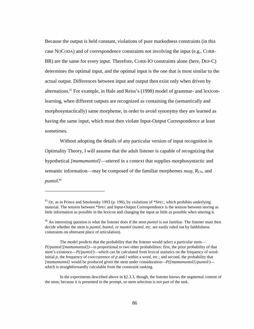
2.7.3. Generating a novel form.................................................................................. 84 2.8. The Listener ........................................................................................................... 85

2.8.1. Introduction ..................................................................................................... 85 2.8.2. Reconstructing the underlying form................................................................ 85 2.8.3. Acceptability judgments.................................................................................. 98

2.9. Chapter Summary................................................................................................. 101 2.10. Appendix: experimental stimuli......................................................................... 103 2.11. Appendix: Calculating probabilities of rankings ............................................... 105

2.11.1. Pairwise ranking requirements .................................................................... 105 2.11.2. Complex ranking requirements ................................................................... 108

2.12. Appendix: Sample calculation in Mathematica ................................................. 111

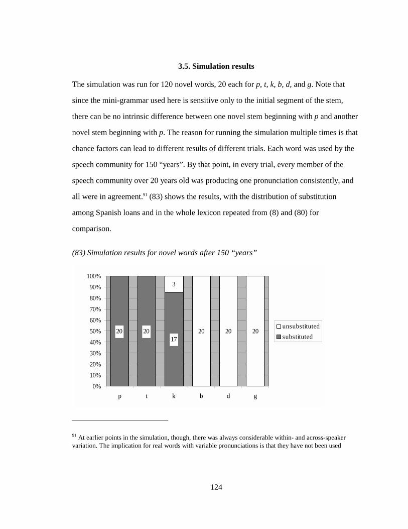
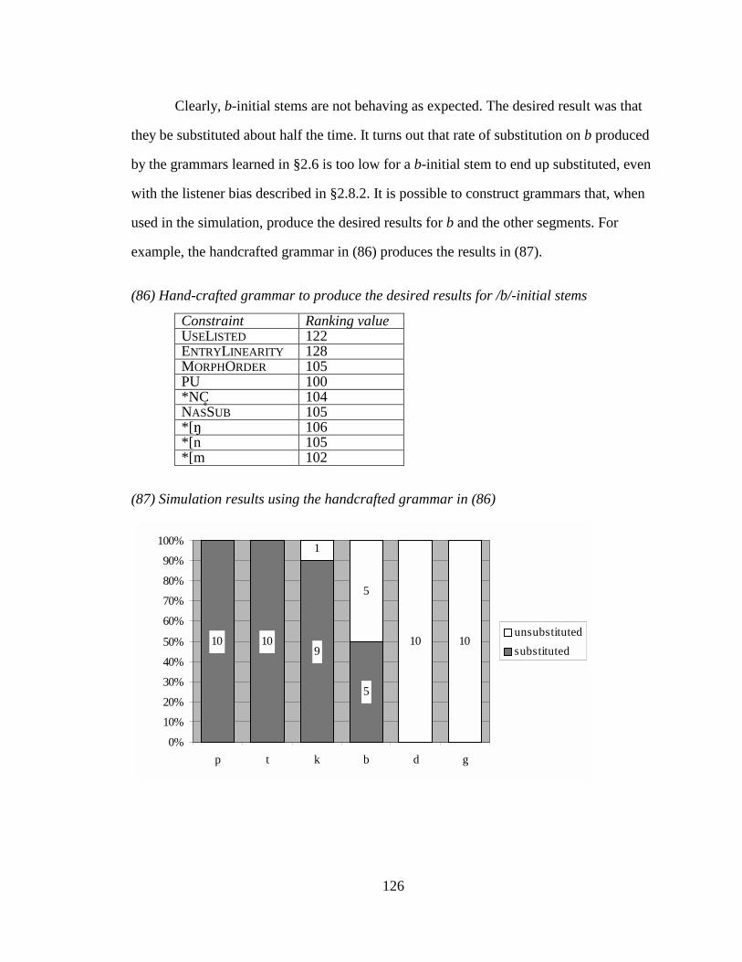
3. Simulating the adoption of a new word................................................................... 114 3.1. Chapter overview ................................................................................................. 114 3.2. Assimilated loanwords ......................................................................................... 114 3.3. Model of the speech community.......................................................................... 118 3.4. How the simulation works ................................................................................... 121 3.5. Simulation results................................................................................................. 124 3.6. Chapter summary ................................................................................................. 127 3.7. Appendix: Functions used in the simulation........................................................ 128

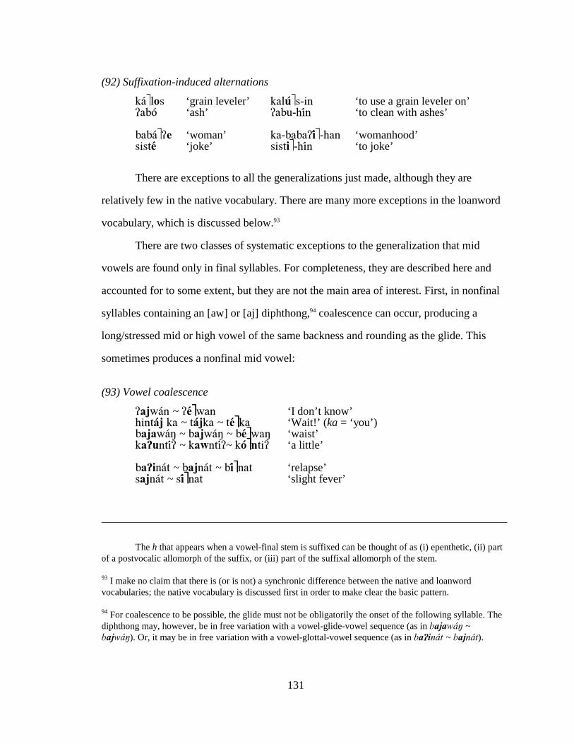
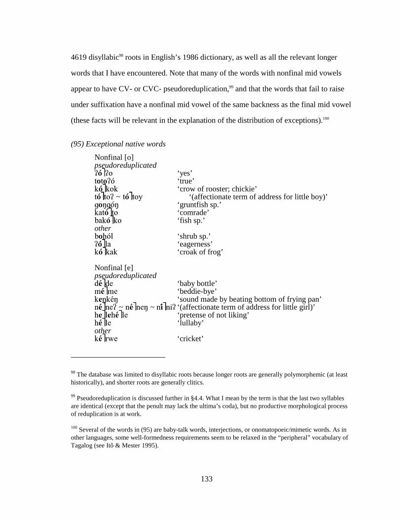
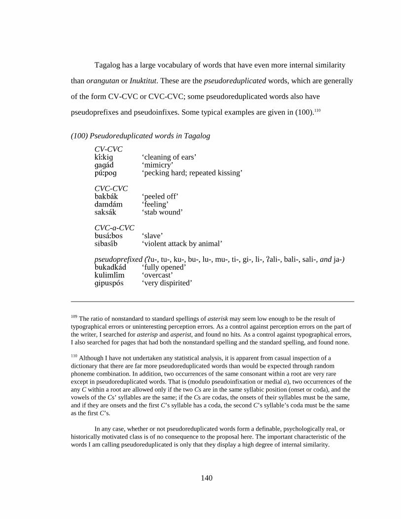
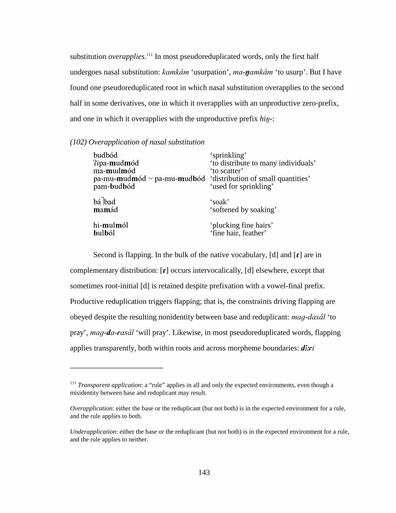
4. The model as applied to vowel height alternations ................................................ 129 4.1. Chapter overview ................................................................................................. 129 4.2. Vowel height in Tagalog...................................................................................... 130 4.3. Analysis of vowel lowering/raising ..................................................................... 135 4.4. Aggressive Reduplication .................................................................................... 139

4.4.1. Analysis ......................................................................................................... 146 4.5. Distribution of exceptions in the loanword vocabulary ....................................... 152

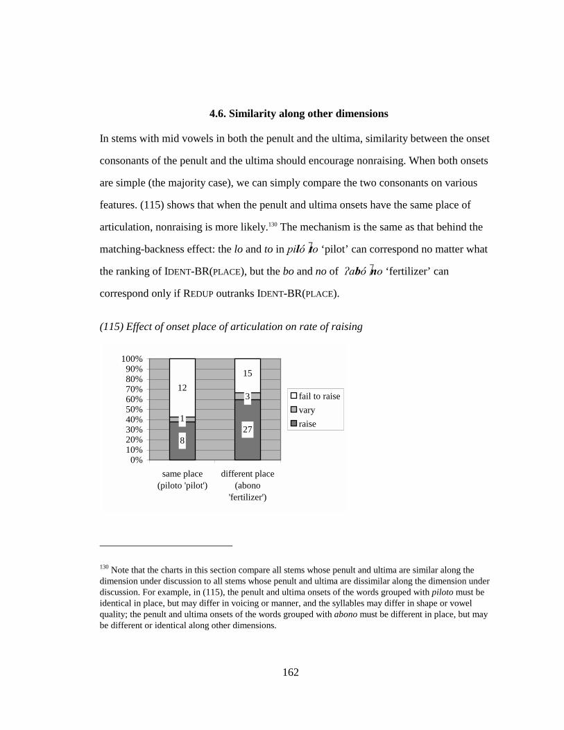
4.5.1. Aggressive Reduplication applied to the vowel raising ................................ 156 4.6. Similarity along other dimensions ....................................................................... 162 4.7. Representations .................................................................................................... 168

4.7.1. Separate entries for derivatives?.................................................................... 168 4.7.2. Environment-tagged allomorphs ................................................................... 169

4.8. Modeling raising .................................................................................................. 175 4.9. Learnability .......................................................................................................... 179 4.10. Chapter summary ............................................................................................... 182 4.11. Appendix: statistical significance of influences on raising................................ 183

5. Alternatives to Encoding Lexical Regularities in the Grammar .......................... 185 5.1. A separate module................................................................................................ 185 5.2. Associative memory............................................................................................. 187 5.3. The dual mechanism model ................................................................................. 190

5.3.1. Evidence for a qualitative difference between irregulars and regulars ......... 192 5.3.2. Why are regular pasts not listed? .................................................................. 195

v

6. Summary .................................................................................................................... 198

References ...................................................................................................................... 200

TABLE OF EXHIBITS

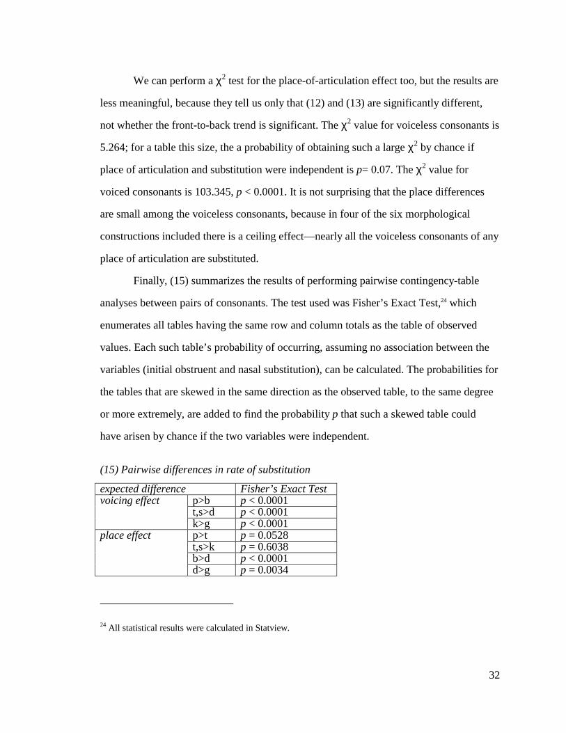
(1) Under- and overspecification......................................................................................... 4 (2) Stress in English words with -ic .................................................................................... 5 (3) English present-past mappings ...................................................................................... 6 (4) Tagalog phoneme inventory ........................................................................................ 12 (5) Examples of Tagalog affixes ....................................................................................... 14 (6) Sample OT tableau ...................................................................................................... 17 (7) Nasal-substituting prefixes with various stems ........................................................... 20 (8) Rates of nasal substitution for entire lexicon............................................................... 23 (9) Rates of substitution for various prefixes .................................................................... 25 (10) Voicing and nasal substitution: observed frequencies............................................... 28 (11) Voicing and nasal substitution: expected frequencies............................................... 28 (12) Place of articulation and nasal substitution: observed frequencies ........................... 30 (13) Place of articulation and nasal substitution: expected frequencies............................ 30 (14) Place of articulation and nasal substitution: (observed-expected)/expected values .. 31 (15) Pairwise differences in rate of substitution................................................................ 32 (16) Differing behavior among derivatives of the same stem........................................... 33 (17) Semantic unpredictability with nasal-substituting affixes......................................... 34 (18) Unpredictable stress/length shifts associated with nasal-substituting affixes ........... 34 (19) Personal characteristics of experiment participants................................................... 36 (20) Sample card for Task I............................................................................................... 37 (21) Sample sentence pair for Task I ................................................................................ 38 (22) Rates of substitution on novel words......................................................................... 40 (23) Overall rates of substitution on novel words, broken down by participant............... 41 (24) Example stimuli for Task II....................................................................................... 42 (25) Acceptability judgments: substituted - unsubstituted; error bars indicate 95%

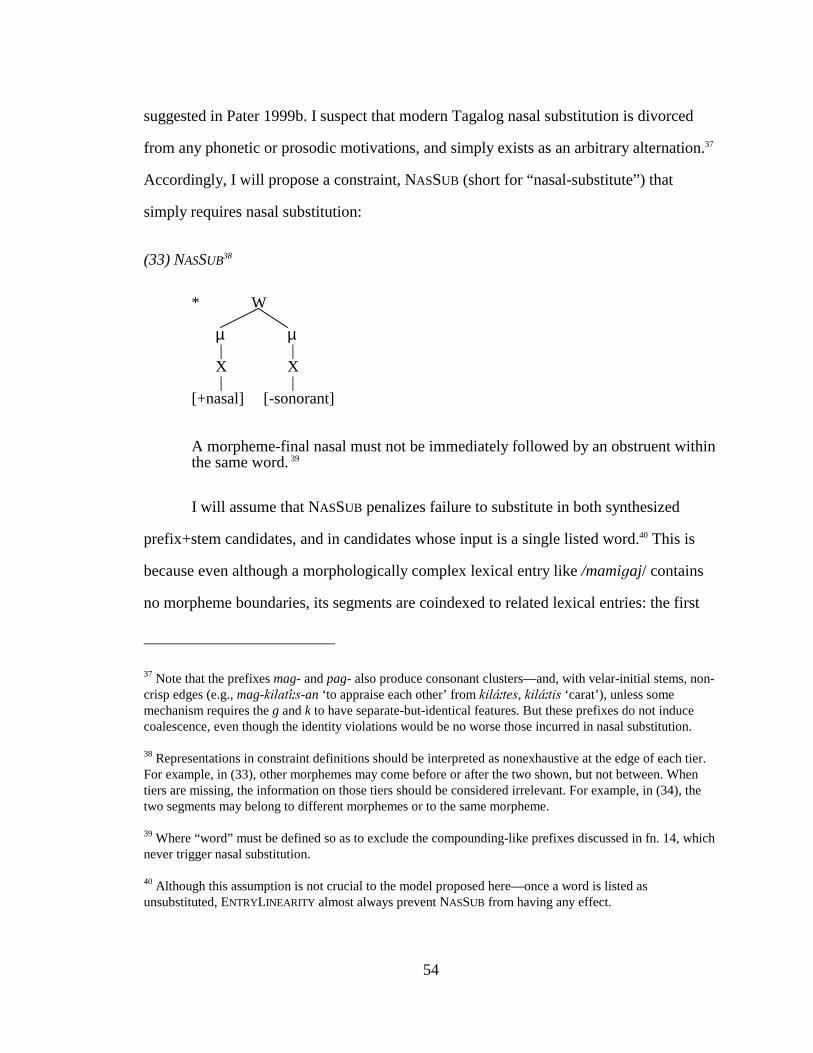
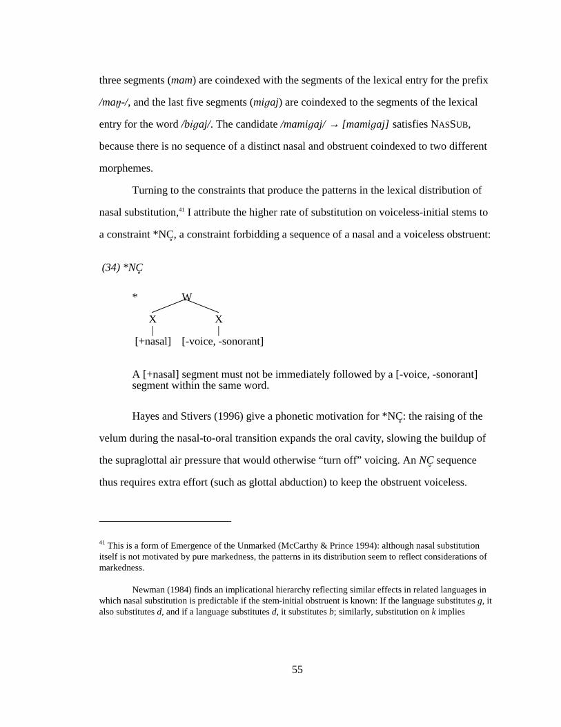
confidence interval .................................................................................................... 43 (26) Nasal substitution as coalescence .............................................................................. 46 (27) Constraints against coalescence................................................................................. 48 (28) Corr-IO constraints: sample violations...................................................................... 49 (29) USELISTED ................................................................................................................. 50 (30) Violations of USELISTED ........................................................................................... 51 (31) Interaction of a family of USEX%LISTED constraints and Paradigm Uniformity ..... 52 (32) Interaction of a unitary USELISTED constraint and Paradigm Uniformity................. 53 (33) NASSUB...................................................................................................................... 54 (34) *NC �............................................................................................................................ 55 (35) Coalescence within vs. across listed items ................................................................ 56

vi

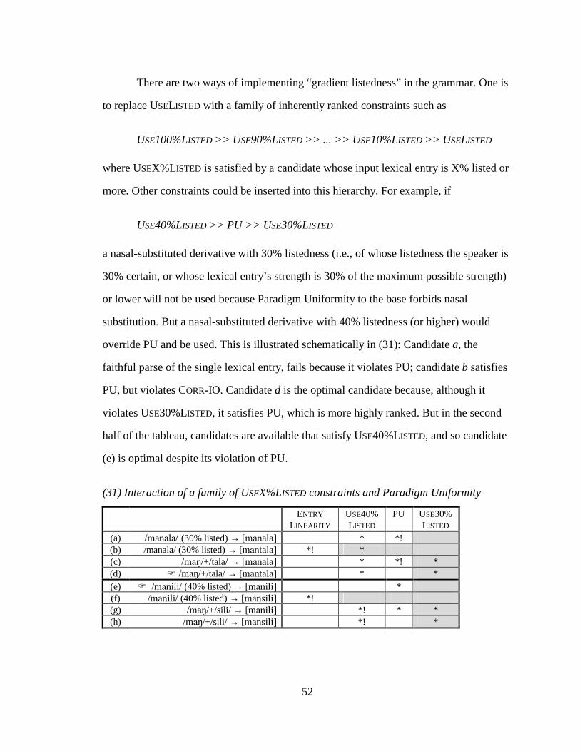
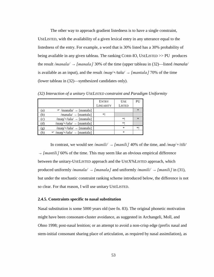
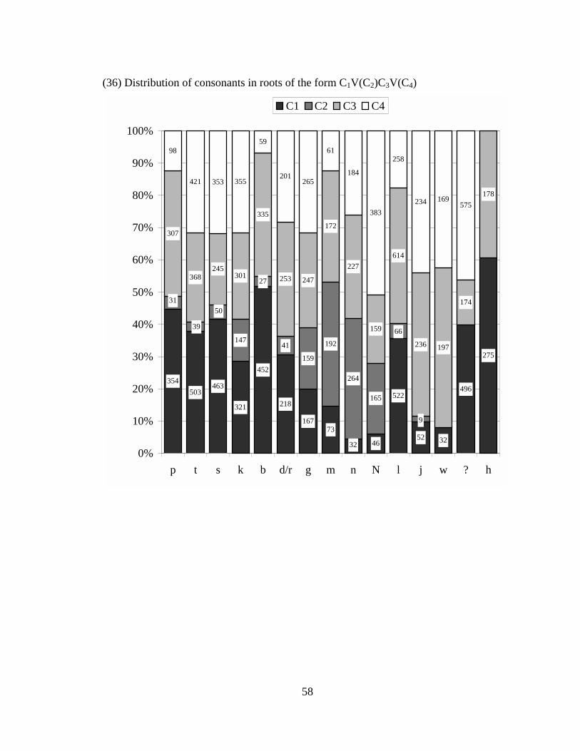
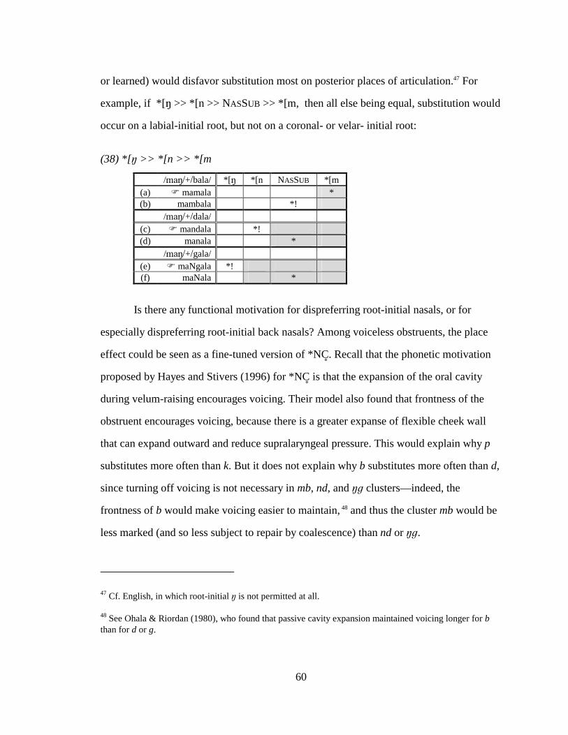
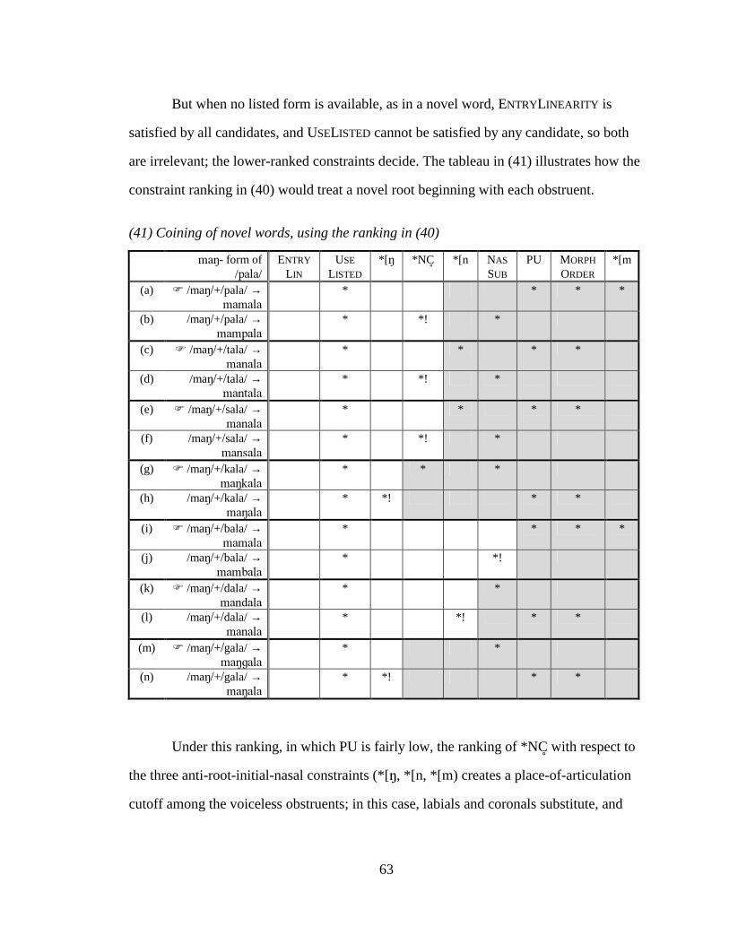
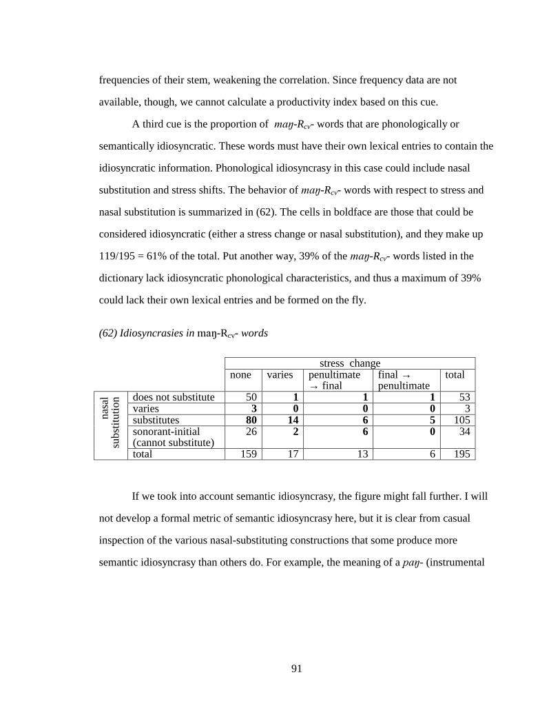
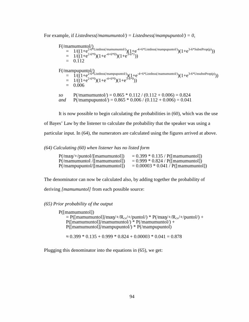
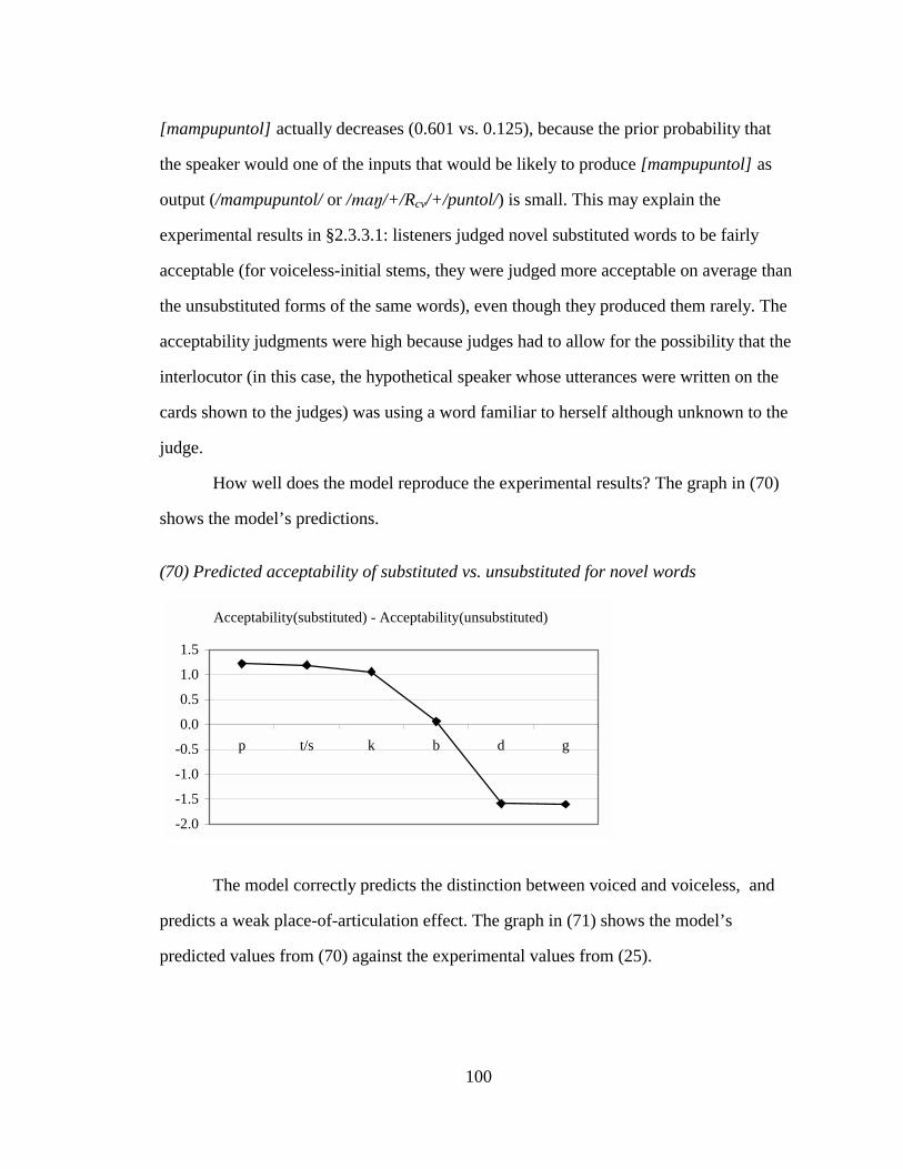
(36) Distribution of consonants in roots of the form C1V(C2)C3V(C4) ............................ 58 (37) *[�, *[n, *[m.............................................................................................................. 59 (38) *[� >> *[n >> *[m..................................................................................................... 60 (39) Constraints affecting nasal substitution..................................................................... 62 (40) Input-Output Correspondence requires use of listed form ........................................ 62 (41) Coining of novel words, using the ranking in (40).................................................... 63 (42) Hypothetical constraint system.................................................................................. 65 (43) Sample lexical entry for stem-listing approach (cf. (16)).......................................... 67 (44) Partial lexical entries for underspecification approach.............................................. 69 (45) Learning, starting with two equally-ranked constraints ............................................ 72 (46) Mini-lexicon for learning........................................................................................... 74 (47) Sample learning trial.................................................................................................. 74 (48) Ranking values arrived at by Gradual Learning Algorithm ...................................... 76 (49) Availability as a function of listedness...................................................................... 78 (50) Hypothetical tableau .................................................................................................. 79 (51) Ranking requirements for candidate a in (50) to be optimal ..................................... 79 (52) Simple hypothetical tableau....................................................................................... 79 (53) Probability of Ci's outranking Cj in a given utterance ............................................... 80 (54) Four candidates for a listed, substituted word ........................................................... 81 (55) Candidate probabilities if /mampupuntol/ exists ....................................................... 83 (56) P(input|output) for various stem-initial obstruents .................................................... 83 (57) Probabilities of outcomes when no listed form exists ............................................... 84 (58) Choosing the optimal input ....................................................................................... 85 (59) Three possibilities on hearing [mamumuntol]........................................................... 87 (60) Bayesian inversion of probabilities compared by listener......................................... 87 (61) P(/���/+/RCV/+/puntol/) = 1/((1+e-3+6*Listedness(whole word))*(1+e3-6*Productivity(���+Rcv)))89 (62) Idiosyncrasies in ���-Rcv- words ............................................................................. 91 (63) Prior probabilities of /mamumuntol/ and /mampupuntol/ ......................................... 93 (64) Calculating (60) when listener has no listed form..................................................... 94 (65) Prior probability of the output ................................................................................... 94 (66) Final result for (64).................................................................................................... 95 (67) Determining the input given output [mampupuntol]................................................. 95 (68) Probability of listener’s guessing that speaker used a listed word: substituted -

unsubstituted.............................................................................................................. 98 (69) P([mamumuntol]) ...................................................................................................... 99 (70) Predicted acceptability of substituted vs. unsubstituted for novel words................ 100 (71) Predicted and experimental acceptability values (substituted - unsubstituted) ....... 101 (72) Novel stimulus stems............................................................................................... 103 (73) Real-word stimulus stems........................................................................................ 104 (74) Mi - Mj ..................................................................................................................... 105 (75) Arriving at a selection point for a constraint in a given utterance........................... 106 (76) Calculating P(Ci>>Cj) ............................................................................................. 106 (77) P(Ci >> Cj) = P(Mi - Mj > -0.5) = .64 ...................................................................... 108

vii

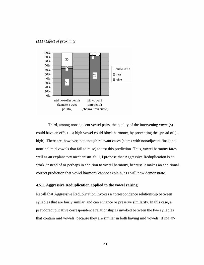
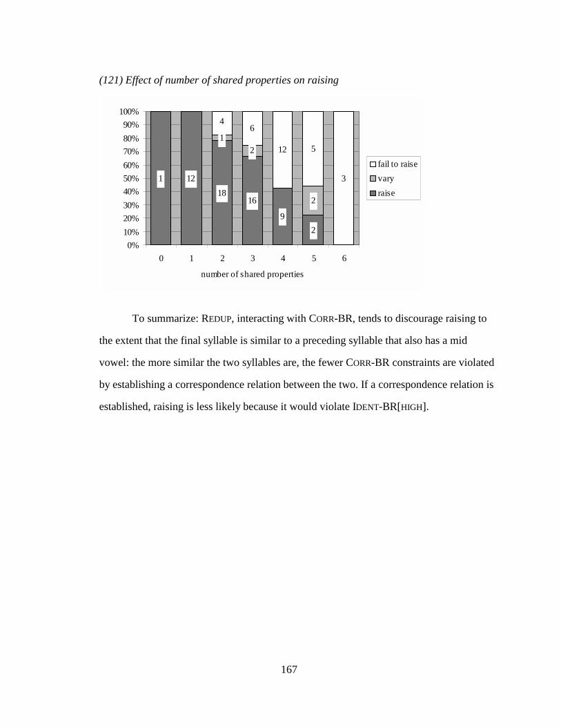
(78) Pairwise rankings are not independent .................................................................... 109 (79) Possible total rankings of three constraints ............................................................. 109 (80) Substitution rates for Spanish stems, all affixal patterns combined ........................ 115 (81) Listener’s procedure for estimating P(output|inputi) ............................................... 122 (82) Estimating P(inputi|output) ...................................................................................... 123 (83) Simulation results for novel words after 150 “years”.............................................. 124 (84) Nasal substitution in real Spanish loans .................................................................. 125 (85) Nasal substitution in entire Tagalog lexicon ........................................................... 125 (86) Hand-crafted grammar to produce the desired results for /b/-initial stems ............. 126 (87) Simulation results using the handcrafted grammar in (86) ..................................... 126 (88) Deciding whether to pay attention to a speaker....................................................... 128 (89) Prior probabilities of inputs (see §2.8.2) ................................................................. 128 (90) Updating listedness.................................................................................................. 128 (91) Distribution of mid and high vowels ....................................................................... 130 (92) Suffixation-induced alternations.............................................................................. 131 (93) Vowel coalescence .................................................................................................. 131 (94) Transglottal vowels.................................................................................................. 132 (95) Exceptional native words......................................................................................... 133 (96) *NONFINALMID ....................................................................................................... 135 (97) *FINAL[u]................................................................................................................. 135 (98) Tableaux illustrating underspecification analysis.................................................... 137 (99) Similarity enhancement in English.......................................................................... 139 (100) Pseudoreduplicated words in Tagalog................................................................... 140 (101) Over- and underapplication in pseudoreduplicated roots ...................................... 142 (102) Overapplication of nasal substitution .................................................................... 143 (103) REDUP .................................................................................................................... 146 (104) Violations of REDUP for a 3-syllable input............................................................ 147 (105) Factorial typology of REDUP, CORR-IO, and CORR-BR ........................................ 148 (106) Loanword stems with nonfinal mid vowels and final [u]...................................... 152 (107) Alternation in loanword stems............................................................................... 152 (108) Effect of mid vowel in penult on probability of raising ........................................ 153 (109) Vowel harmony as a mechanism for preventing alternation ................................. 155 (110) Effect of matching backness between penult and ultima, given a mid penult....... 155 (111) Effect of proximity ................................................................................................ 156 (112) Aggressive reduplication blocks vowel raising ..................................................... 157 (113) A ranking that prevents correspondence between mismatched vowels ................ 158 (114) Vowel non-raising in CV reduplication................................................................. 160 (115) Effect of onset place of articulation on rate of raising .......................................... 162 (116) Effect of onset manner on rate of raising .............................................................. 163 (117) Effect of onset voicing on rate of raising .............................................................. 164 (118) Effect of onset shape on rate of raising ................................................................. 164 (119) Effect of rhyme shape on rate of raising................................................................ 165 (120) Effect of vowel length on raising .......................................................................... 166 (121) Effect of number of shared properties on raising .................................................. 167

viii

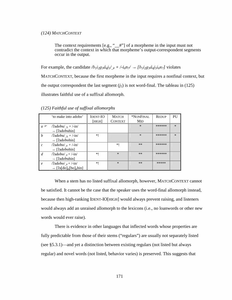
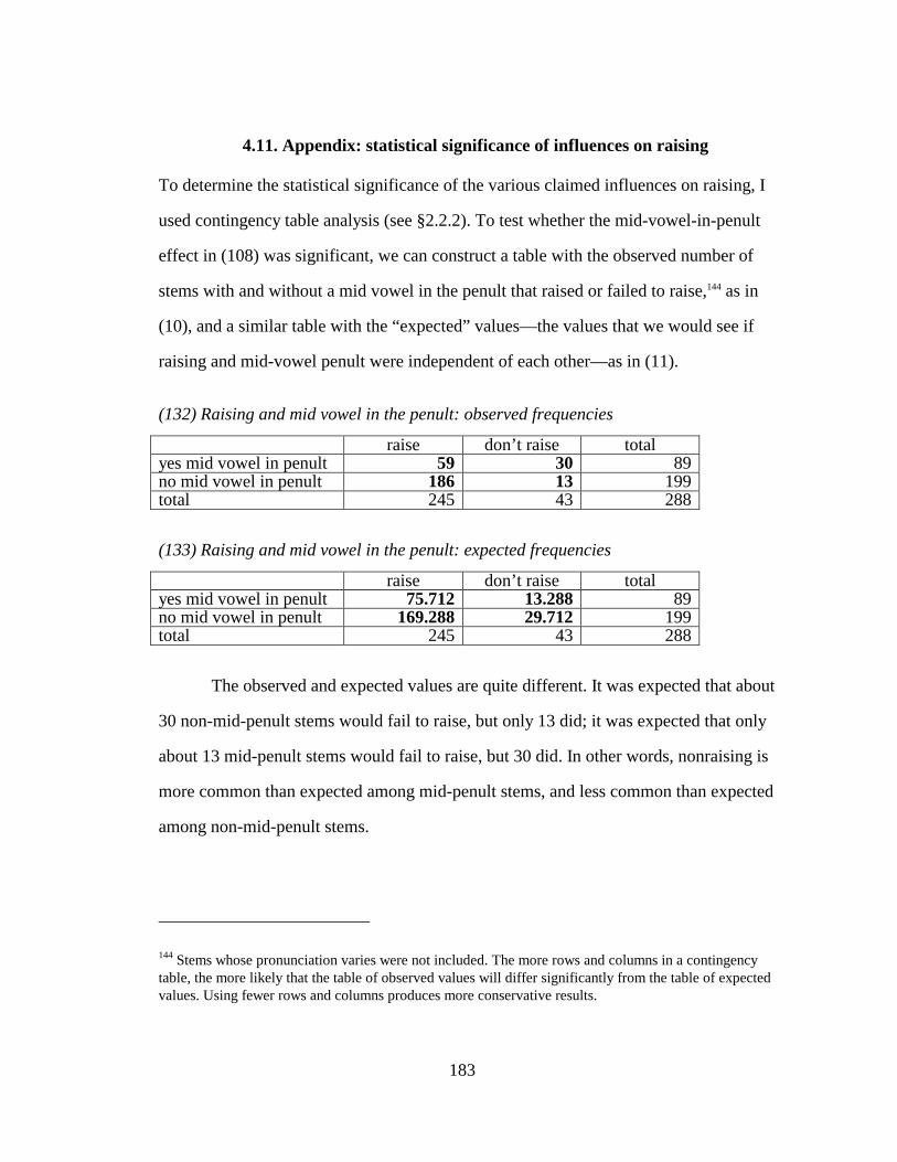
(122) Syncope ................................................................................................................. 170 (123) Suffixal allomorphs—sample partial lexical entries ............................................. 170 (124) MATCHCONTEXT.................................................................................................... 171 (125) Faithful use of suffixal allomorphs........................................................................ 171 (126) Variability for constructed suffixal allomorphs..................................................... 173 (127) Vowel height in a novel word: identical syllables................................................. 176 (128) Vowel height in a novel word: similar syllables ................................................... 176 (129) Vowel height in a novel word: dissimilar syllables............................................... 177 (130) Grammar used in simulation.................................................................................. 181 (131) Rate of raising in novel words with mid penults, using the grammar in (130) ..... 181 (132) Raising and mid vowel in the penult: observed frequencies ................................. 183 (133) Raising and mid vowel in the penult: expected frequencies ................................. 183 (134) Statistical significance of various inhibitors of vowel raising............................... 184

ix

ACKNOWLEDGMENTS

First I have to thank Bruce Hayes and Donca Steriade, my advisers. They’ve been the

best thing (among many very fine things) about my six years here at UCLA. Just about

everything I know, they taught me, and certainly any good idea I’ve ever had has come

from a conversation with one of them. And without their encouragement to follow my

nose, this would have been a much tamer dissertation, for better or for worse. I hope

Bruce and Donca realize that they’re my role models in all areas of life. I doubt I can ever

live up to the example they’ve set as scholars, teachers, and mentors, but at least I know

what to shoot for.

I asked Carson Schütze to be on my committee because I knew he’d ask hard

questions, and he did. I know I haven’t really answered all of them, but trying to answer

them has clarified my thinking a lot, and I think made this a better work. I asked Donka

Minkova to be on my committee because of its diachronic flavor; thanks to her for giving

me an informed perspective on my claims about lexical change and the role of

interactions in the speech community.

What first attracted me to UCLA was the sense of excitement among the students

and faculty over what they were doing. Sustaining that environment requires time and

effort, and I’d like to thank all of the students and faculty in this department for the

interaction that has been invaluable to me. Particularly to be thanked are Adam Albright,

Dan Albro, Marco Baroni, Roger Billerey, Katherine Crosswhite, Janine Ekulona,

Christina Foreman, Matt Gordon, Bruce Hayes, Sun-Ah Jun, Pat Keating, Ed Keenan,

Robert Kirchner, Peggy MacEachern, Pam Munro, Carson Schütze, Ed Stabler, Donca

Steriade, Siri Tuttle, and Jie Zhang.

x

This dissertation draws mainly on data from Tagalog. I was first introduced to the

language in a field methods course at McGill taught by Lisa Travis, with Natividad del

Pilar as language consultant. Tania Azores-Gunter was my Tagalog teacher for two years

at UCLA, and I’m grateful to her for her patience and encouragement. Thanks to all the

Tagalog speakers who shared their knowledge of the language with me, especially Nenita

Pambid-Domingo and Angel Camandang.

Over the years I’ve been fortunate to have many outstanding teachers. I would

have been lucky to study with just one of them; to have so many to thank is a wonder.

From my years at FACE, I should Frank Cottam for introducing me to linguistics and

Iwan Edwards for the lesson that what’s worth doing is worth doing well. At the

University of Illinois Laboratory High School, David Bergandine, Chris Butler, Mort

Castle (who didn’t work at Uni, but taught me while I was there), Sandra Dawson,

Elizabeth Jokusch, Peter Kimball, Rosemary Laughlin, Pat McLaughlin, Rick Murphy,

Frances and John Newman, Bernard Norcott, Al Smith, David Stone, and Joanne

Wheeler provided an atmosphere of constant intellectual stimulation, encouraged

thorough and systematic thought, and generally made us feel that anything was possible.

At McGill, Heather Goad, Myrna Gopnik, and Glynne Piggott helped me begin to

become a linguist by treating me as though I already was one.

Finishing graduate school isn’t the hardest thing in the world, but it takes its toll.

Katherine Crosswhite, Leah Gordon, and Peggy MacEachern provided friendship that I

couldn’t have done without, as did Linda and Phil Ross, my first teachers and most loyal

supporters. And anyone who knows me knows that I would never have made it through

without the aid and comfort of Bryan Zuraw. He gave me constant encouragement,

tolerated my mood swings and mounting paranoia, and, as the pace of work on this

xi

document accelerated, took over all my non-dissertation responsibilities and made sure I

had clean clothes every morning and a hot meal every night.

xii

VITA

March 29, 1973 Born, Montreal, Quebec, Canada 1990-1994 James McGill Entrance Scholarship McGill University Montreal, Quebec, Canada 1992 Sarah Rosenfeld Prize in Yiddish McGill University 1993 Betty Workman Yaffe Prize in Yiddish McGill University 1994 Undergraduate Research Assistant Familial Language Impairment Project McGill University 1994 B. A. with First Class Honours, Linguistics McGill University 1994-1996 Bourse de maîtrise en recherche

Fonds pour la Formation de Chercheurs et l’Aide à la Recherche

1994-1997 National Science Foundation Graduate Fellowship 1995-1999 Teaching Assistant, Associate, Fellow Department of Linguistics University of California, Los Angeles 1996 M. A., Linguistics University of California, Los Angeles Los Angeles, California 1996-1997 Phonetics Laboratory Computer Assistant Department of Linguistics University of California, Los Angeles 1997-1998 Teaching Assistant Consultant Department of Linguistics University of California, Los Angeles 1998 Instructional Software Programmer Department of Linguistics University of California, Los Angeles 1999 Dissertation Year Fellowship University of California, Los Angeles

xiii

PUBLICATIONS AND PRESENTATIONS

Zuraw, Kie (April 1996). Moving Phonotactics: Variability in Infixation and Reduplication of Tagalog Loanwords. Paper presented at the Third Annual Meeting of the Austronesian Formal Linguistics Association, Los Angeles, California.

Zuraw, Kie (April 1998). Tagalog Nasal Substitution: Allomorphic Emergence of the Un-

marked. Paper presented at the Southwest Workshop on Optimality Theory, Tucson, Arizona.

Zuraw, Kie (January 1999). Knowledge of Lexical Regularities: Evidence from Tagalog

Nasal Substitution. Paper presented at the Annual Meeting of the Linguistic Society of America, Los Angeles, California.

Zuraw, Kie (June 1999). Regularities in the Polymorphemic Lexicon. Invited paper

presented at the Workshop on the Lexicon in Phonetics and Phonology, University of Alberta, Edmonton, Alberta, Canada. To appear in proceedings.

Zuraw, Kie (January 2000). Aggressive Reduplication in Tagalog. Paper presented at the

Annual Meeting of the Linguistic Society of America, Chicago, Illinois. Zuraw, Kie (February-March 2000). Patterned Exceptions in Phonology. Invited

colloquium presented at the University of California, Los Angeles; the University of Southern California; and the University of California, Irvine.

Zuraw, Kie (to appear). Regularities in the Polymorphemic Lexicon. University of

Alberta Papers in Experimental and Theoretical Linguistics 8.

xiv

ABSTRACT OF THE DISSERTATION

Patterned Exceptions in Phonology

by

Kie Ross Zuraw

Doctor of Philosophy in Linguistics

University of California, Los Angeles, 2000

Professor Bruce Hayes, Co-chair

Professor Donca Steriade, Co-chair

Standard Optimality-Theoretic grammars contain only the information necessary

to transform inputs into outputs; regularities among inputs are not accounted for. Using

the example of Tagalog nasal substitution, this dissertation presents a model of how

lexical regularities could be learned, represented in the grammar, used by speakers and

listeners, and perpetuated over time.

Lexical regularities are represented as low-ranking constraints, their rankings

learned through exposure to the lexicon using Boersma’s Gradual Learning Algorithm.

High-ranked constraints ensure the primacy of listed pronunciations; but when a speaker

produces a novel word, these high-ranking constraints are irrelevant and the constraints

that encode lexical regularities take over. The subterranean constraints are stochastically

ranked; speakers’ behavior on novel words probabilistically reflect the lexical

regularities. The listener uses the same grammar to produce well-formedness judgments

for novel words and to reconstruct inputs from an interlocutors’ outputs. The model’s

xv

well-formedness judgments reproduce the experimental result that although the

productivity of nasal substitution on novel words is low, nasal-substituted novel words

are judged more acceptable than non-substituted words in certain cases.

Bayesian reasoning by the listener favors novel nasal-substituted words—they are

disproportionately likely to become listed. A computer simulation of the speech

community confirms that although nasal substitution is the minority pronunciation for

novel words, a word may eventually enter the lexicon as nasal-substituted.

Tagalog vowel raising under suffixation is close to exceptionless in the native

vocabulary but quite exceptionful among loanwords. A loan stem’s probability of

resisting raising is highly influenced by its degree of internal similarity. I propose that

internal similarity encourages speakers to construe a word as reduplicated, even without

morphosyntactic motivation; raising is blocked because it would disrupt base-reduplicant

identity.

Alternatives to encoding lexical regularities in the grammar are considered. It is

argued that the vowel raising facts are not amenable to an associative memory account.

The qualitative difference between “regulars” and “exceptions” cited by proponents of

the Dual-Mechanism model as evidence for leaving lexical regularities out of the

grammar reduces to a difference between listed words and synthesized words; this

difference can arise through listener reasoning, without a prior qualitative difference.

xvi

1

1. Introduction

This dissertation presents a model of how phonological patterns in the lexicon could be

learned and used by speakers and hearers, and perpetuated over time. This chapter

introduces the phenomenon of lexical patterns, discusses why they are problematic in

current phonological thinking, and gives a preview of the model.

1.1. Lexical regularities

I will use the terms lexical regularity and phonological pattern to refer to generalizations

about the phonological properties of the set of words in a language. Regularities can be

observed that apply within morphemes, within morphologically complex words, and

across sets of words.

1.1.1. Regularities within morphemes

In English roots of the form sCVC, the two Cs generally cannot be both labial, both velar,

both nasal, or both [l].1 The generalization is quite strong (see Berkley 1994 for statistical

findings on this and related phenomena in the English lexicon), and hypothetical

exceptions, though pronounceable, sound somewhat ill-formed (?[����], ?[���]).2

Generalizations like this one are often attributed to morpheme structure constraints

1 Although such sequences are common across word or morpheme boundaries: It’s Lily! or Ask Angry Joe.

2 A search of the online Oxford English Dictionary for sCVC words only (i.e., not the full set of sC(C)VC(C) words, which follow similar restrictions) found, collapsing variant spellings and pronunciations, just 3 words with two labials (Spam, spume, spoom), 9 words with two velars (skoke, skeck, skowke, skeg, skig, scak, scoke, scag, scug), 3 words with two nasals (smon, snam, snum), and no words with two ls. Most of these words were unfamiliar to me.

2

(introduced by Halle 1959 as “morpheme structure rules”)3—language-specific

conditions that rule out some set of possible morphemes as ill formed.

Morpheme structure constraints are static in the sense that they can be observed

only as a property of existing words; they do not drive alternations. Although slill sounds

strange, it is pronounceable and does not require any “repair”.

Morpheme structure constraints are rarely exceptionless. For example, English

words like [��Θ�] ‘Spam (brand name of processed meat product)’ and [����] ‘skeg (oat

species; part of ship’s keel; fin of surfboard; plum species; nail; stump of a branch; tear in

cloth)’ violate the sCVC restriction described above. There needs to be some mechanism

that allows these words to escape the constraint.

1.1.1.1. Zimmer’s conundrum

What is the role of morpheme structure constraints in the grammar, since they do not

drive alternations? In Optimality Theory (OT; see §1.5), often include a proof that the

correct surface forms result no matter what the input (Richness of the Base: Prince &

Smolensky 1993, Smolensky 1996a). For example, if a language lacks morphemes of the

form CiVCi, the analysis includes a demonstration that the input /pop/ is repaired to (say)

[pot]. A problem with this type of demonstration, of course, is that the analyst generally

does not know what the correct surface form for the input /pop/ should be ([pok], [kop],

[po]...)—it might even be [pop].

In the case of morpheme structure constraints at least, it is doubtful that such

proofs are necessary, because the learner has no reason to posit underlying forms that are

significantly different from the surface forms. For example, by Lexicon Optimization

(Prince & Smolensky 1993; Itô, Mester, & Padgett 1995), the learner would construct the

3 although root structure constraint would be more apt in most cases.

3

underlying form /pok/ for a morpheme that is always pronounced [pok]; similarly, she

would construct /kop/ for [kop], and so on. If she never hears [pop], she will not

construct /pop/, and so there is no need for the grammar to repair /pop/, because no such

lexical entries exist. If the constraint against morphemes of the form CiVCi plays no role

except to repair inputs that may not exist anyway, then perhaps it does not belong in the

grammar.

Inkelas, Orgun, and Zoll 1997 make a similar argument for Labial Attraction, a

constraint on vowels in Turkish roots.4 Inkelas et al. propose a overspecification as a

mechanism for tagging words as exceptions to constraints. Nonexceptional segments in

morphemes are underspecified, and their feature values can be filled in by markedness

constraints at no faithfulness cost. In different morphological contexts, different values

will be filled in, resulting in alternation. Exceptional segments, on the other hand, are

fully specified, and high-ranked faithfulness constraints prevent tampering with those

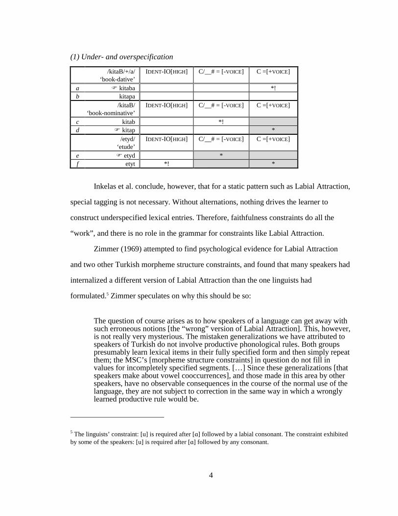
underlying specifications. The tableau in (1) illustrates the analysis for Turkish final

devoicing: underspecified /kitaB/ (B stands for a bilabial stop unspecified for voicing)

undergoes final devoicing, but overspecified /etyd/ does not.

4 Labial Attraction is a systematic exception to Round Harmony: normally, a high vowel must agree in [round] with a preceding vowel (e.g., *�tu), but if the preceding vowel is [�] and the intervening consonant is labial, then a high, back vowel will be [+round] instead of [-round] as expected. Round Harmony drives alternations, applying across a suffix boundary, but Labial Attraction holds only within morphemes (and even within morphemes, there are exceptions).

4

(1) Under- and overspecification

/kitaB/+/a/ ‘book-dative’

IDENT-IO[HIGH] C/__# = [-VOICE] C =[+VOICE]

a � kitaba *! b kitapa /kitaB/

‘book-nominative’

IDENT-IO[HIGH] C/__# = [-VOICE] C =[+VOICE]

c kitab *! d � kitap * /etyd/

‘etude’

IDENT-IO[HIGH] C/__# = [-VOICE] C =[+VOICE]

e � etyd * f etyt *! *

Inkelas et al. conclude, however, that for a static pattern such as Labial Attraction,

special tagging is not necessary. Without alternations, nothing drives the learner to

construct underspecified lexical entries. Therefore, faithfulness constraints do all the

“work”, and there is no role in the grammar for constraints like Labial Attraction.

Zimmer (1969) attempted to find psychological evidence for Labial Attraction

and two other Turkish morpheme structure constraints, and found that many speakers had

internalized a different version of Labial Attraction than the one linguists had

formulated.5 Zimmer speculates on why this should be so: The question of course arises as to how speakers of a language can get away with such erroneous notions [the “wrong” version of Labial Attraction]. This, however, is not really very mysterious. The mistaken generalizations we have attributed to speakers of Turkish do not involve productive phonological rules. Both groups presumably learn lexical items in their fully specified form and then simply repeat them; the MSC’s [morpheme structure constraints] in question do not fill in values for incompletely specified segments. […] Since these generalizations [that speakers make about vowel cooccurrences], and those made in this area by other speakers, have no observable consequences in the course of the normal use of the language, they are not subject to correction in the same way in which a wrongly learned productive rule would be.

5 The linguists’ constraint: [u] is required after [�] followed by a labial consonant. The constraint exhibited by some of the speakers: [u] is required after [�] followed by any consonant.

5

The conundrum is, if Labial Attraction does no “work” in the grammar of

Turkish, why had speakers internalized any version of it at all?

1.1.2. Regularities within morphologically complex words

Regularities are also to be found in morphologically complex words. For example,

English words suffixed with -ic generally have penultimate stress, regardless of the stress

pattern in the base.

(2) Stress in English words with -ic

artíst-ic cf. ártist laparoscóp-ic cf. láparoscope cholerá-ic cf. chólera

There are a few exceptions to this generalization, such as chóler-ic (cf. chóler) and Árab-

ic (cf. Árab).

Regularities in polymorphemic words are “productive” in the sense that if a

speaker knows only the related base, it is up to her to create a word that follows or does

not follow the generalization. (By contrast, if a speaker knows the word slill, she has no

choice but to pronounce it slill.) For example, should the -ic form of carob be carób-ic or

cárob-ic (or something else)? Compared to morpheme structure constraints, regularities

in polymorphemic words thus have more opportunity to make themselves felt in the

language, as new affixed forms are coined much more frequently than new morphemes.

Regularities in morphologically complex words might seem at first glance to

naturally belong in the grammar (and so Zimmer’s conundrum would not arise), but when

there is evidence that the words are listed as separate lexical entries (see §2.2.3), the

situation is the same as with morpheme structure constraints: speakers would not need to

6

learn the regularity in order to produce existing words correctly. But if speakers do apply

the regularity to novel affixed words, this fact must be accounted for somehow.

1.1.3. Regularities across words

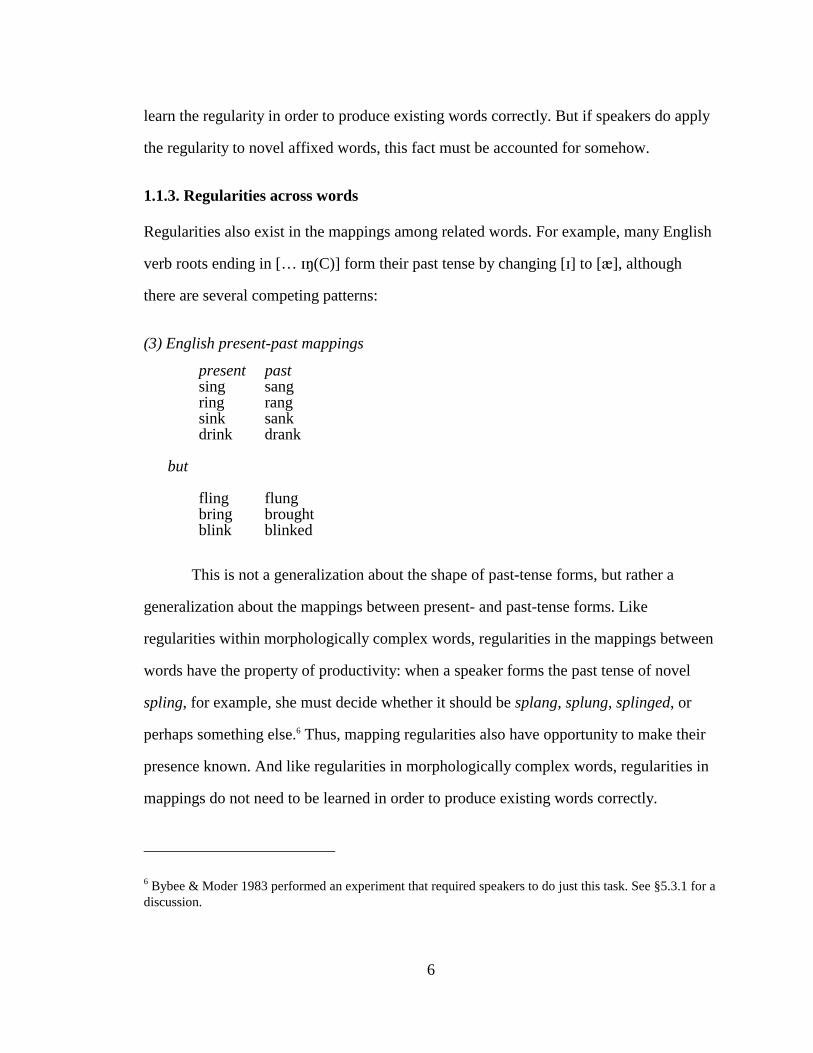
Regularities also exist in the mappings among related words. For example, many English

verb roots ending in [… ��(C)] form their past tense by changing [�] to [], although

there are several competing patterns:

(3) English present-past mappings

present past sing sang ring rang sink sank drink drank

but

fling flung bring brought blink blinked

This is not a generalization about the shape of past-tense forms, but rather a

generalization about the mappings between present- and past-tense forms. Like

regularities within morphologically complex words, regularities in the mappings between

words have the property of productivity: when a speaker forms the past tense of novel

spling, for example, she must decide whether it should be splang, splung, splinged, or

perhaps something else.6 Thus, mapping regularities also have opportunity to make their

presence known. And like regularities in morphologically complex words, regularities in

mappings do not need to be learned in order to produce existing words correctly.

6 Bybee & Moder 1983 performed an experiment that required speakers to do just this task. See §5.3.1 for a discussion.

7

1.2. Exceptions to lexical patterns

It was mentioned above that lexical regularities tend to have exceptions (Spam, Árabic,

blinked), but the distribution of exceptions often is not random. In the two cases

discussed in this dissertation (Chapters 2 and 4), the exceptions themselves are highly

patterned: although it is not predictable whether any given word will be an exception,

words with certain phonological properties are more likely than others to be exceptions.

There are not enough exceptions to the sCVC morpheme structure constraint or to the

generalization that -ic carries penultimate stress to look for patterns within the

exceptions, but we can see many such patterns in English past tense. For example, a verb

is more likely to follow the [�]-[] mapping if it has a velar nasal in the coda than if it has

an alveolar or bilabial nasal (begin, began; swim, swam) (see Bybee & Slobin 1992 for a

discussion of regularities in the distribution of English past-tense mappings).

Frisch, Broe, and Pierrehumbert (1996), expanding on Pierrehumbert 1993,

examined the distribution of exceptions to an Arabic morpheme structure constraint that

forbids consonants of the same place of articulation within a root. They showed that far

from being random, exceptions to the constraint are distributed such that the more similar

two consonants are, the less likely they are to cooccur. For example, /t...d...k/ and

/t...z...k/ both violate the constraint against homorganic consonants within a root, but

because t and d are more similar than t and z (they share membership in more natural

classes), roots of the form /t...d...X/ are more common than roots of the form /t...z...X/.

Frisch et al.’s account of the Arabic facts is discussed in the following section. See Frisch

and Zawaydeh (to appear) for evidence on the psychological reality of this constraint.

8

1.2.1. Regularities in a separate system: the Stochastic Constraint Model

The Stochastic Constraint Model (Frisch, Broe, & Pierrehumbert 1996, Frisch 1996) is an

attempt to model lexical regularities. Frisch et al. propose constraints that are functions

from phonological characteristics to acceptability values, which should predict

experimental well-formedness judgments and lexical frequency.7 The functions are of the

form acceptability = 1/(1+eK+Sx), where x is the numerical value of the phonological

characteristic, and K and S are parameters that determine the location and sharpness of

the boundary between acceptable and unacceptable.

To account for the Arabic constraint, a function is proposed that takes as its x the

similarity between two consonants and returns an acceptability value between 0 and 1.8

The acceptability value was compared against lexical frequency, and the match was

found to be good. Frisch 1996 compared this model to several others and found that it

was a better fit to the Arabic lexicon.

The Stochastic Constraint Model models knowledge of well-formedness, and

explains patterns in the distribution of exceptions to morpheme structure constraints. But

constraints in this model play a very different role from that of constraints in OT. To

quote Frisch 1996, “[the stochastic constraint] does not influence what the output is for

7 The mechanism relating well-formedness and lexical frequency in unclear, but we can say there is a two-way relationship. On the one hand, lexical frequency shapes acceptability values by determining what values the learner assigns to the parameters of the stochastic constraint. On the other hand, acceptability values could shape lexical frequency by influencing how rare words or loans are “repaired” (low-acceptability words would tend to drift towards repairs that enhance their acceptability), and influencing the shape of newly coined words.

8 This is somewhat of a simplification. First, the function is acceptability = A/(1+eK+Sx), where A need not be 1. In directly modeling lexical frequency (observed number of occurrences/expected number of occurrences) without the mediating step of acceptability, Frisch 1996 uses other values of A to get a better fit. Second, Frisch 1996 actually multiplies together three different constraints to get a total acceptability value: one constraint is a function on the similarity of the first two consonants in a triliteral, one is on the similarity between the second and third, and one is on the similarity between the first and third.

9

any particular input, but rather it constrains the space of possible inputs and outputs in a

probabilistic manner.” (p. 92) The mental system represented by the Stochastic

Constraint Model would have to exist alongside the system for mapping inputs to outputs.

This dissertation proposes a model in which the same system that maps inputs to outputs

can encode lexical regularities and patterns in the distribution of exceptions to those

regularities.

1.3. Preview of the proposal

It is conceivable that knowledge of lexical regularities resides outside the grammar—or

even that no discrete knowledge of the regularities exists at all. Speaker behavior that

appears to reflect such knowledge could merely be the result of some on-line procedure

such as consultation of a sample of the lexicon or matching to associative memory. These

two strategies are discussed at greater length in Chapter 6 and shown to be ill suited to

the regularities discussed in this dissertation. As argued there, the speaker must possess

knowledge that is abstracted away from the lexicon itself. The only linguistic subsystem

commonly proposed that contains such knowledge is the grammar. Therefore, the

approach taken here will be to incorporate knowledge of lexical regularities directly into

the grammar.

To accomplish that goal, this dissertation proposes a model of grammar that

allows the primacy of listed information to coexist with knowledge of lexical regularities.

Existing words’ behavior is encoded in their lexical entries; that information is preserved

through high-ranking faithfulness constraints and constraints that force listed information

to be used if available. Lexical regularities are encoded through low- and variably ranked

constraints, which are irrelevant for existing words, but determine the pronunciation of

novel words.

10

The ranking tendencies of these subterranean constraints are learned through

exposure to the lexicon, using Boersma’s (1998) Gradual Learning Algorithm, which is

shown to be capable of learning rates of lexical variation: constraints that are violated by

many words become low-ranked, and constraints that are violated by few words become

high-ranked, even if none of those constraints are relevant for existing words once the

grammar reaches its adult state (in this case, because high-ranking faithfulness constraints

determine the optimal candidate).

Chapter 2 presents Tagalog nasal substitution, a sporadic morphophonemic

phenomenon. A statistical examination of the lexicon reveals that the distribution of

exceptions to nasal substitution is patterned. Experimental evidence is presented for the

psychological reality of nasal substitution and its subregularities. The chapter implements

the model for the case of nasal substitution, showing how the subterranean constraints

governing nasal substitution and its patterns produce rates of substitution on novel words

and acceptability ratings for novel words that are similar to the experimental results. In

particular, the paradoxical result that speakers perform nasal substitution at a low rate on

novel words, but rate certain types of nasal-substituted novel words as highly acceptable

is explained in terms of the listener’s probabilistic reasoning about her interlocutor’s

underlying form (in rating a novel word, the listener must entertain the possibility that for

her interlocutor, the word is not novel).

Chapter 3 shows how probabilistic interactions between speakers and listeners

perpetuate lexical patterns as new words enter the language. Bayesian reasoning on the

part of the listener results in a bias in favor of nasal-substituted pronunciations: although

they are the minority pronunciation for a novel word, listeners disproportionately tend to

add them to their lexicons (whereas unsubstituted pronunciations tend to be ignored). The

chapter presents the results of introducing novel words into a computer-simulated speech

11

community, attempting to replicate the rates of substitution for various stem types that

can be observed in Spanish loans.

Chapter 4 applies the model to vowel height alternations in Tagalog. Although

vowel raising under suffixation is nearly universal in native words, many loanwords from

Spanish and English have resisted raising. The chapter argues that the main predictor of

whether a word will resist raising is how amenable it is to being construed as reduplicated

(raising is then prevented, because it would disrupt reduplicative identity). It is argued

that a purely phonological mechanism (Aggressive Reduplication) drives such

morphosyntactically unmotivated reduplicated construals. This second case is of interest

because the subregularity involved is quite abstract, and does not emerge

straightforwardly from associative memory.

1.4. Tagalog

Because nearly all the data discussed in the body of this dissertation are from Tagalog,

this section covers some essential facts about the language, and gives details on how

lexical data were obtained. Although this dissertation’s main goal is to present a model of

lexical regularities, I hope that it will also be useful as a source of detailed information on

several aspects of Tagalog phonology.

Tagalog (Austronesian, Malayo-Polynesian, Western Malayo-Polynesian, Meso

Philippine, Central Philippine, Tagalog) is the national language of the Philippines (in

this role, it is sometimes called Pilipino). It has over 15 million first-language speakers

worldwide (Ethnologue 1996), and is used to some degree by 39 million Pilipinos. First-

language speakers are mainly in Luzon and Mindoro.

The language has long had contact to varying degrees with Chinese, Malay, and

languages of Indonesia and India; a moderate number of loanwords from these languages

12

are still in use. During the time of the Spanish occupation of the Philippines (mid

sixteenth through nineteenth centuries), there was extensive contact with Spanish;

starting with the U.S. occupation (first half of the twentieth century) and continuing to

today there has been extensive contact with English. There are now large numbers of

loanwords from Spanish and English.

1.4.1. Phonology sketch

The phoneme inventory of Tagalog is given in (4).

(4) Tagalog phoneme inventory

� �� �� � � � �� � ��� �� �� �� � � � �� � ��� � �� � �� � � � ��� �� �� ��� � ��� � ��� �� ��

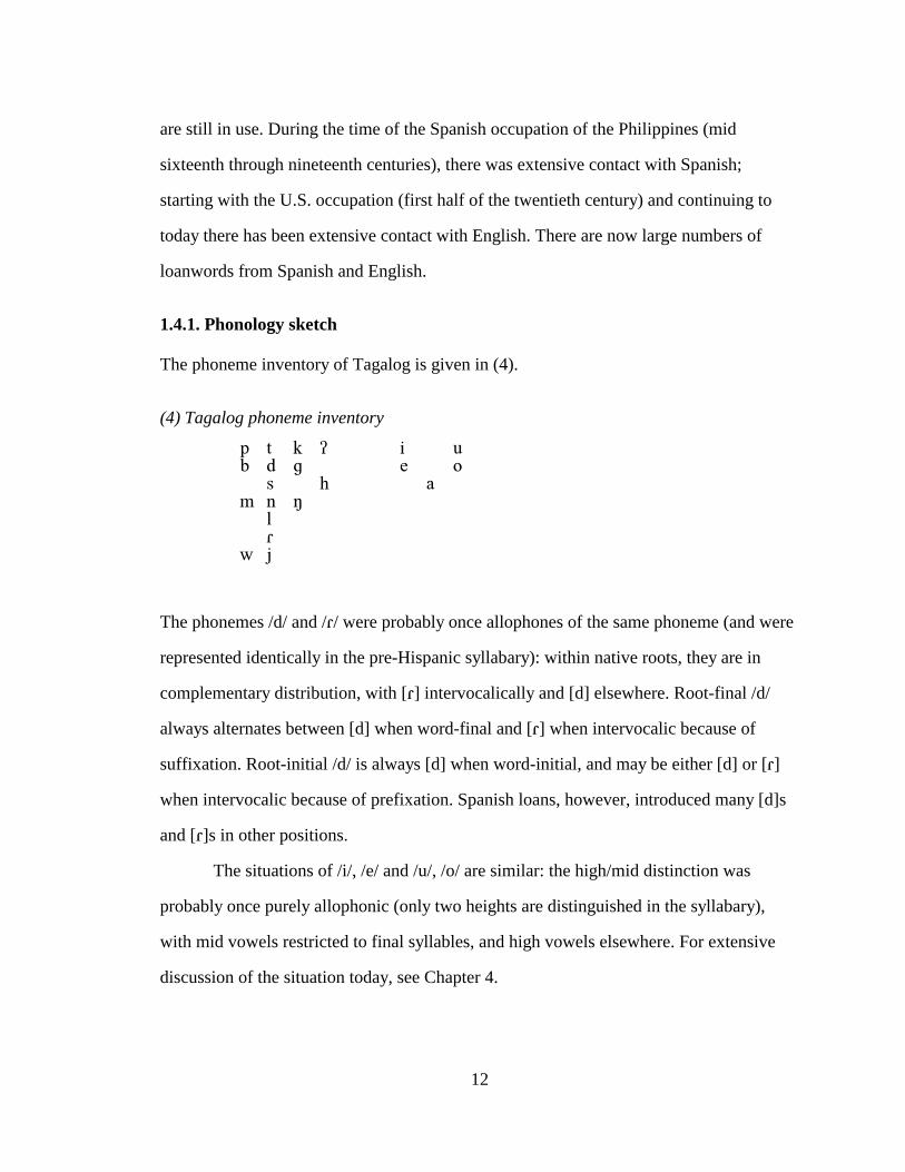
The phonemes /d/ and /�/ were probably once allophones of the same phoneme (and were

represented identically in the pre-Hispanic syllabary): within native roots, they are in

complementary distribution, with [�] intervocalically and [d] elsewhere. Root-final /d/

always alternates between [d] when word-final and [�] when intervocalic because of

suffixation. Root-initial /d/ is always [d] when word-initial, and may be either [d] or [�]

when intervocalic because of prefixation. Spanish loans, however, introduced many [d]s

and [�]s in other positions.

The situations of /i/, /e/ and /u/, /o/ are similar: the high/mid distinction was

probably once purely allophonic (only two heights are distinguished in the syllabary),

with mid vowels restricted to final syllables, and high vowels elsewhere. For extensive

discussion of the situation today, see Chapter 4.

13

Other sounds are frequently used in loanwords, such as [�], [��], [��], [��] and

sometimes [f].

The basic syllable structure is CV(C), although onset clusters are commonly

found in loanwords, and coda clusters occasionally. Most roots are disyllabic. Either

stress or length is contrastive.9 I will not take a position on which (for two opposing

views, see e.g. Schachter & Otanes 1972 and French 1988), and both are marked in all

examples (long vowels with no marked stress are secondary-stressed).

Tagalog is rich in morphology. There are many derivational prefixes, which are

often stacked several deep. There are two inflectional (and sometimes derivational)

infixes, -in- and -um-, which are inserted between the first C and V of the stem (the result

may be a verb, noun, or adjective depending on the construction).10 There are two

suffixes, -in and -an, which also play a variety of roles. When a vowel-final word is

suffixed, the allomorphs -hin and -han are used. There is also reduplication: the first C

and V can be copied (usually inflectional; I refer to this as REDCV), or the first two

syllables (derivational). Some examples of Tagalog affixes are shown in (5).

9 There are two types of word: those with a long, stressed penult, and those with a short penult and a stressed ultima. There are a few loans that some speakers pronounce with antepenultimate stress and length. In native words, a long/stressed penult must be open, but in some loans, it is closed. In derived words, there may be length and secondary stress on the antepenult or earlier syllables.

10 In loans with complex onsets, the position of the infix varies (between the two onset consonants or between the onset and nucleus). See Ross 1996.

14

(5) Examples of Tagalog affixes

bare stem: ����� ‘size, bulk’ prefixation: ��-����� ‘big’ ��-��-��-����� ‘smug’ infixation: l-um-���� ‘to grow big’ suffixation: ����-����11 ‘to enlarge (object focus12)’ reduplication: ���-����� ‘will grow big’ � � � � ��-�����-����� ‘fairly large’

1.4.2. Notes on the data

Tagalog data of three types are presented: experimental data, lexical statistics, and

examples. The experimental data are discussed in detail in §2.3. The lexical statistics are

based on English (1986), a two-volume Tagalog-English, English-Tagalog dictionary.

The dictionary was compiled by Leo English, a (non-native speaker of Tagalog) priest

who lived in the Philippines for 30 years, and Teresita Castillo, a native speaker of

Tagalog. The exact methods for determining which pronunciations to include are not

known, and probably involved consensus among Castillo and the several other Tagalog

speakers who assisted. Because of the large size of the corpus and the frequent

disagreement among speakers as to the correct pronunciation of individual words, the

dictionary was used as the sole source of lexical statistics, producing a large, consistent

11 also lak-����. See §4.7.2 for a discussion of syncope.

12 Every Tagalog sentence (with a few exceptions) has what may loosely be called the focus: a noun phrase that bears the enclitic si (for proper names of people) or ����(for all other noun phrases); the other noun phrases in the sentence bear the enclitic kaj/sa (if indirect object, goal, etc.) or ni/��� (if direct object or subject). There are also corresponding focus and nonfocus pronouns. The verbal morphology indicates the thematic role of the focused noun phrase. For example, in a sentence with the verb laki-����, the object being enlarged would be marked with ���, the person enlarging it with ni, and the instrument being used to enlarge with sa. See Schachter & Otanes 1972 for a thorough description of Tagalog syntax.

15

source of pronunciations. Thus, although an individual word discussed in Chapter 2

might be pronounced with nasal substitution (see §2.2.1) by some speakers and without

by others, the overall statistics should be representative of the speech community.

Examples given in the text are drawn from English’s dictionary, from reference

sources such as Schachter and Otanes 1972 and Ramos and Bautista 1986, and from my

own observations of spoken and written Tagalog. I am not a native (or even fluent)

speaker of Tagalog, but have studied the language both as a linguist and in the classroom.

Transcriptions are IPA (Handbook of the International Phonetic Association

1999), with the exception that an acute accent is used to indicate stress. In some tables

and charts, where phonetic fonts were not available, “N” is used for [�], “?” for [ ], and

“r” for [�]. Tagalog orthography is also used in some tables and charts; it is identical to

IPA except that “ng” is used for [�], “r” for [�], and “y” for [j], and [ ] is not written.

1.5. Appendix: OT basics

The analytical framework used here is Optimality Theory (OT: Prince & Smolensky

1993). The machinery of Correspondence Theory (McCarthy & Prince 1995) is also

employed extensively. It is not possible of course to give a complete explanation of

Optimality Theory here, but a brief overview is possible. See Archangeli and Langendoen

1997 or Kager 1999 for a full introduction to OT.

OT employs two functions, Gen and Eval. Gen takes an underlying representation

(“input”) and returns a (possibly infinite) set of possible surface forms (“output

candidates”). Some output candidates might be identical to the input, others slightly

modified (for example by deleting one segment), others unrecognizable. Eval chooses the

candidate that best satisfies a set of ranked constraints; this optimal candidate becomes

16

the surface representation. The ranked constraints are violable, in the sense that the

optimal candidate may still violate some constraints.

The constraints are of two types: Markedness constraints enforce well-formedness of

the output itself, for example by forbidding consonant clusters. Faithfulness constraints

enforce similarity between the input and the output, for example by requiring all input

segments to appear in the output.

In standard OT, the constraint set is strictly ranked: a candidate that violates a high-

ranking constraint more than other candidates do can never redeem itself by satisfying

lower-ranked constraints. Eval can be thought of as choosing the subset of candidates that

violates the top-ranked constraint the fewest times, then of this subset, selecting the sub-

subset that violates the second-ranked constraints the fewest times, and so on until only

one candidate remains.

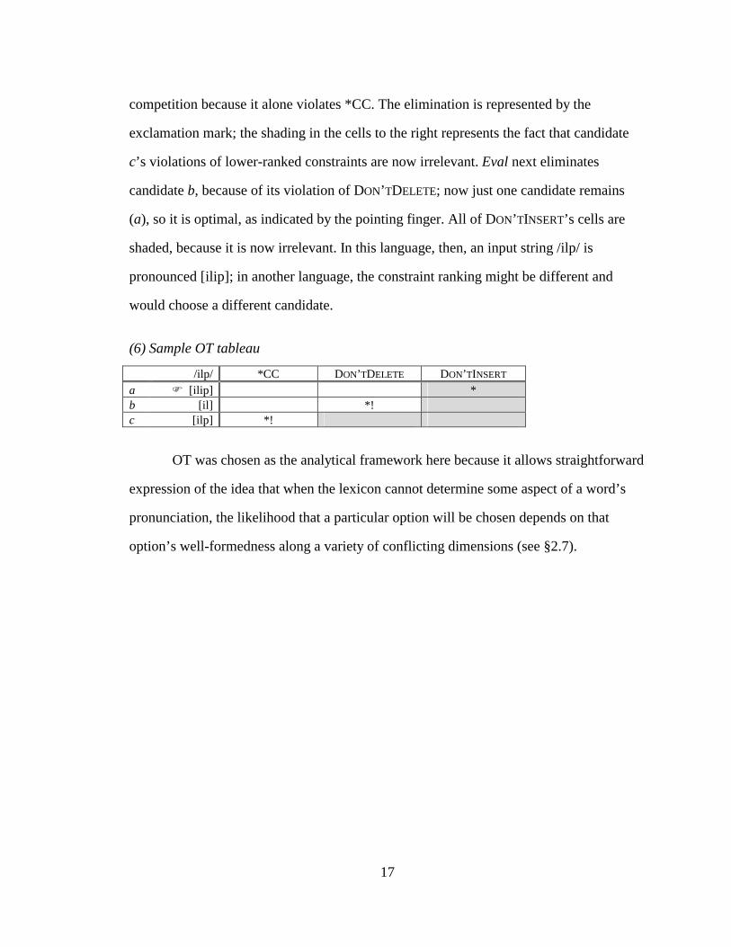
The “tableau” (a standard expositional device in OT) in (6) illustrates this procedure

for the input /ilp/ (upper left corner) in a hypothetical mini-language. Each of the output

candidates a, b, and c is flawed in some way: c, the candidate that looks most like the

input, has a consonant cluster; this violates the constraint against consonant clusters,

*CC, as indicated by the asterisk in the cell at the intersection of *CC’s column and

candidate c’s row. *CC is a Markedness constraint. Candidate b has deleted a segment,

and candidate a has inserted a segment; these candidates violate the Faithfulness

constraints DON’TDELETE and DON’TINSERT, respectively.13

In this language, *CC is the highest-ranked constraint (ranking is indicated by left-to-

right ordering of the constraints’ columns—we can also write

*CC>>DON’TDELETE>>DON’TINSERT). Eval first eliminates candidate c from the

13 These two constraint names are shorthands. See §2.4.3 for some standard constraint names and definitions.

17

competition because it alone violates *CC. The elimination is represented by the

exclamation mark; the shading in the cells to the right represents the fact that candidate

c’s violations of lower-ranked constraints are now irrelevant. Eval next eliminates

candidate b, because of its violation of DON’TDELETE; now just one candidate remains

(a), so it is optimal, as indicated by the pointing finger. All of DON’TINSERT’s cells are

shaded, because it is now irrelevant. In this language, then, an input string /ilp/ is

pronounced [ilip]; in another language, the constraint ranking might be different and

would choose a different candidate.

(6) Sample OT tableau

/ilp/ *CC DON’TDELETE DON’TINSERT a � [ilip] * b [il] *! c [ilp] *!

OT was chosen as the analytical framework here because it allows straightforward

expression of the idea that when the lexicon cannot determine some aspect of a word’s

pronunciation, the likelihood that a particular option will be chosen depends on that

option’s well-formedness along a variety of conflicting dimensions (see §2.7).

18

2. The model as applied to nasal substitution

2.1. Chapter overview

This chapter presents a model of lexical regularities through the example of nasal

substitution in Tagalog. Section 2.2 describes the phenomenon of nasal substitution and

its distribution in the lexicon. Section 2.3 presents the results of an experiment aimed at

assessing the psychological reality of nasal substitution in production and judgment of

well-formedness. Section 2.4 gives a grammar for nasal substitution, with constraints that

encode the regularities in its distribution. Section 2.5 considers several possibilities for

how potentially nasal-substituting words are represented in the lexicon. Section 2.6

shows how the grammar in §2.4 could be learned from exposure to the lexicon, using

Boersma’s (1998) Gradual Learning Algorithm. Section 2.7 describes the speaker’s

probabilistic use of the grammar for novel and existing words. Finally, §2.8 describes

how the listener uses the grammar to determine her interlocutor’s underlying form and to

arrive at acceptability judgments.

19

2.2. Nasal Substitution

2.2.1. The phenomenon

Nasal substitution is a phenomenon that occurs somewhat sporadically in the Tagalog

lexicon. When certain prefixes are attached to a stem beginning in a sonorant, they appear

as ���-, ���-, or, less often, na�-, which is derived morphologically from ���-.14 (e.g.,

���� ‘army’, ���-���� ‘military’). But when these same prefixes attach to an

obstruent-initial stem, either they appear with place assimilation to the obstruent, as ���-

/�� -/���-, ���-/�� -/���-, ��-/ � -/ ��- (e.g., ������ ‘district’, ���-������

‘local’), or the final nasal of the prefix and the obstruent appear to combine into a nasal

that is homorganic to the original obstruent (e.g., ���-������ ‘give’, ��-������

‘distribute’). It is the second case that is known as nasal substitution. In (7) are shown

examples, for every consonant in the Tagalog inventory, of substitution and

14 There are a variety of productive morphological constructions that participate in nasal substitution, but in all of them, the prefix complex ends in ���-, ��-, or ���- (even though, morphosyntactically, it may be preferable to think of the affixes as a whole, since the meaning of the prefix complex is often not compositional). There are also some unproductive constructions that can trigger nasal substitution, whose prefix complexes end in, ��-, ��- � �-, � �- (the only common one), ���-, and ���- (e.g., � ����� ‘number’, �-� ���� ‘digit’; ��� �� ‘upside-down’, �-��� �� ‘return’; ������� ‘leader’, � -������ ‘grammatical subject’; ����� ‘louse’,�� -�����-� � ‘to pick out lice’; ����� ‘corpse’, ��-����-��� ‘death’; ������ ‘descent’,���-��-��-������ ‘humble’). The fairly productive construction mag-���-RCV, for verbs of accidental result (������ ‘face down’, mag-kan-da-������� ‘to fall on one’s face’), never produces substitution.

This set exhausts the prefixes that end in �, except for a group that I do not consider real prefixes, because they seem more like members of a compound: ������-, (� )����-, (��)� �-, ��� ��- and �� ��- (e.g., ������� ‘payment’ ������-������� ‘free’; ����� � ‘finger-width’ ���-����� � ‘one finger width’; � � ‘black’, ��� ��-� � ‘as black as’; ������ ‘fruit’ ��� � ��-������ ‘conversion into a fruit’; ������� ‘vinegar’ �� ��-��������‘to become vinegar’). These are all two syllables long (except for optionally shortened (� )����- and (��)� �-), can bear their own stress, produce semantically transparent words, never induce nasal substitution, and often fail to undergo nasal assimilation. In addition, ������ ‘does not have/exist’ and � ���� ‘one’ also occur as free-standing words, which require the “linker” -�- under certain circumstances.

20

nonsubstitution, using a variety of common morphological constructions that can trigger

substitution.

(7) Nasal-substituting prefixes with various stems

� �������� ‘grief’ �-��-�������� ‘being in grief’ �� ��� ‘district’ ��-�� ��� ‘local’ � ��- ������� ‘staying as guest’ ���-�-�������-�� ‘fellow lodger’ ������ ‘driving forward’ ��-������ ‘to goad’ � ������� ‘usurpation’ ��-�-������� ‘rapacious’ ��������� ‘scales’ ��-��������� ‘tool for removing scales’ � ����� ‘fish’ ���-��-������ ‘fisher’ ������ ‘silly’ ���-������ ‘to fool someone’ � ���-������ ‘to give’ ��-������ ‘to distribute’ ������� ‘pronouncing’ ���-��-������� ‘reciter’ �� �������� ‘prayer’ �-�-������-�� ‘to pray’ ����� ‘audible’ ��-����� ‘sense of hearing’ �� �������15 ‘unsteadiness on feet’ �-��-������� ‘unsteadiness on feet’ ������� ‘witchcraft’ ���-��-������ ‘witch’ �� �������� ‘writing’ ���-��-������ ‘writer’ � � � � � � � � � ��-�������� � � � ‘writing instrument’��� ����� ‘army’ ��- ����� ‘military’ �� ��!��� ‘mark’ ��-��!��� ‘marker’ (no examples of n16) �� ������ ‘grinding of teeth’���-��-������ ‘grinding of teeth’ �� ������� ‘ration’ ��-�������, ��-������� ‘for rationing’ �� ������ ‘assimilation’ ��-��-������ ‘monopolistic’ � ��� -������ ‘to sprinkle’ ��-������ ‘sprinkler’ � ������ ‘annoyance’ ���-������ ‘to annoy’

A few remarks on the examples in (7): First, when nasal substitution occurs in

conjunction with reduplication, both base and reduplicant are substituted (��-��-

����������rather than *��-��-��������� or *��-��-����������); when no nasal substitution

occurs, the assimilated nasal precedes only the reduplicant (���-��-��������rather

than�*���-��-��������). I adopt Wilbur’s (1973) and McCarthy and Prince’s (1995)

15 One of only 2 instances of substitution of g that I found.

16 Nasal-initial roots are few in Tagalog. The absence of any n-initial roots that have potentially nasal-substituting derivatives is probably accidental.

21

proposal that “overapplication” of nasal substitution in ��-��-����������results from

reduplicative correspondence. Note that the overapplication shows that a nasal resulting

from substitution belongs to the stem (although it may also belong to the prefix in some

sense; see the discussion of coalescence in §2.4), whereas a prefix nasal that merely

assimilates is not part of the stem.

Second, it is not clear whether nasal substitution is possible on nasal-initial stems:

nasal-initial stems are rare to begin with, and among those that do exist, it is not always

possible to tell what the prefix is. For example, in ma-�� ���� ‘to become numb’, from

�� ���� ‘numb’, it is not clear whether the prefix is simply ma- (which can also form

verbs, with similar semantics), or ���- with nasal substitution.17 There do exist

unambiguous constructions (such as ���+REDUPLICATION—there is no potentially

confusable ma+REDUP), but no cases of nasal-initial stems in these constructions.

Third, glottal stop is problematic. Many researchers have assumed that initial

glottal stop in Tagalog is simply predictably inserted in vowel-initial words (since there

are no strictly vowel-initial words); the preservation of initial glottal stop in prefixed

words like mag-������� ‘to fight’ (or ��������) would then be regarded as the effect of a

tendency to align morpheme boundaries with syllable boundaries (for a formal theory of

alignment, see McCarthy & Prince 1993, Cohn & McCarthy 1998). And a word like

17 Schachter and Otanes (1972) argue that these verbs are ��-prefixed, because their gerunds are formed by changing m to p and reduplicating, as are the gerunds of uncontroversially ��-prefixed verbs (���� ‘fear’, ma-������ ‘to intimidate’, pa-na-������ ‘intimidating’). In contrast, ma- verbs’ gerunds are formed by replacing ma- with pagka- (��-����� ‘to get involved’, �����-����� ‘getting involved’). But Carrier (1979) points out that some m → p & RCV gerunds do come from ma- verbs (pa-li-� ����� ‘bathing’ from ma-� ����� ‘to take a bath’).

Carrier (1979) argues against the ��-with-substitution analysis for nasal-initial stems, because some of the nasal-initial stems that take ma-/��- do not substitute when combined with ���-, and so should not substitute with ��- (���-������ ‘for watching’). But, I have found many stems that substitute with ��- but not with ���- (����� ‘tail end’, ma-���� ‘to finish last’, pam-����� ‘tailpiece’).

22

������������ would be failure of alignment rather than true nasal substitution, either with

the nasal of the prefix becoming associated to the stem, or with reduplicative

correspondence causing the second � to be inserted.18 Since glottal stop is phonemic

word-finally, I prefer to regard word-initial glottal stop as phonemic rather than

epenthetic (why pick glottal stop as the epenthetic segment rather than something else?),

and I view ������������ as nasal-substituted, although, as will be seen below, the

distribution of “substituted” glottal stops in the lexicon is puzzling.

2.2.2. Distribution of exceptions

I collected all 1,736 words from English (1986) that had an obstruent-initial stem and a

potentially nasal-substituting prefix, and found two trends. First, substitution is most

likely with a front stem-initial consonant (p or b) and least likely with a back consonant

(k or g). Second, substitution is more likely if the stem-initial consonant is voiceless than

if voiced. Both trends can be seen in (8), which combines data from all constructions (t

and s are also combined, to better illustrate the two trends; t and s are separated in the

more detailed charts that follow). 19

18 A similar proposal, considered and rejected by Carrier (1979), is that there is a phonemic difference between truly glottal-stop-initial and truly vowel-initial stems, which determines whether or not nasal substitution will appear to occur. Thus � ����� would be underlyingly / �����/, and �������underlyingly /������/. There are some glottal/vowel-initial stems whose derivatives vary in whether or not they substitute, but this does not refute Carrier’s idea: such stems would be underlyingly vowel-initial, but in some derivatives morpheme-specific alignment constraints would force an epenthetic glottal stop.

19 Previous accounts of the lexical distribution of nasal substitution have noted (not quite correctly) that g never substitutes (Bloomfield 1917, Schachter & Otanes 1972); that d and g rarely substitute (Blake 1925); that voiceless consonants substitute more than voiced ones (De Guzman 1978, but see fn. 20); and that morphology matters (Schachter & Otanes 1972, De Guzman 1978).

23

(8) Rates of nasal substitution for entire lexicon

Different constructions have different overall substitution rates. The bar charts in

(9) show rates of substitution for each stem-initial obstruent in the most common affix

patterns. The breakdown by affix is suggested in part by De Guzman (1978), who

distinguished adversative from nonadversative verbs,20 and instrumental adjectives (������

‘writing’, pa- ����� ‘used for writing’) from reservative adjectives (������� ‘banquet’,

pam-������� ‘for a banquet (said of clothes, food, etc.)’).21

20 Adversative verbs are hostile or harmful to the patient (e.g., ���� ‘stone’, ma-�� � or mam-��� � ‘to throw stones at’). Nonadversative verbs include inchoatives (����� ‘thin’, ma-���� ‘to become thin’), statives (�� � �� ‘teeming with’, ma-� � �� ‘to teem with’), professional verbs (���� ‘medicine’, ��-���� ‘to practice medicine’), habitual verbs (� ��� ���� ‘cigarette’, ma-� ��� ���� ‘to be a smoker’), distributives (k-um-����� ‘get’, ma-������ ‘to gather things’), and repetitives (� ������ ‘window’, ma- ������ ‘to keep looking out a window’).

21 De Guzman claimed that in non-adversative verbs, substitution is obligatory for all obstruents and that in adversative verbs, substitution is obligatory for voiceless Cs but optional for voiced Cs and glottal stop. (9) shows that there are some counterexamples to the first clause of the claim; although the classification of some verbs could be argued over, there are some nonsubstituting verbs that are definitely nonadversative

253 430 185 177 25

70 97

1

10100

26 17

0%10%20%30%40%50%60%70%80%90%

100%

p t/s k b d gstem-initial obstruent

perc

enta

ge o

f wor

ds th

at su

bstit

ute

unsubstitutedsubstituted

24

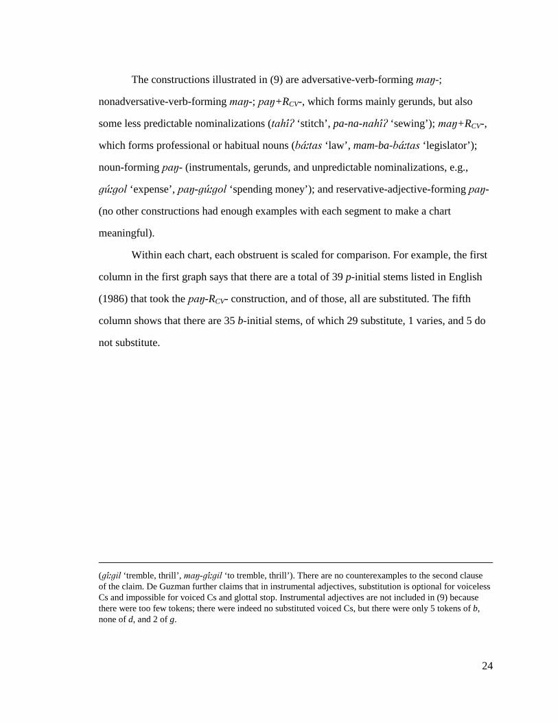
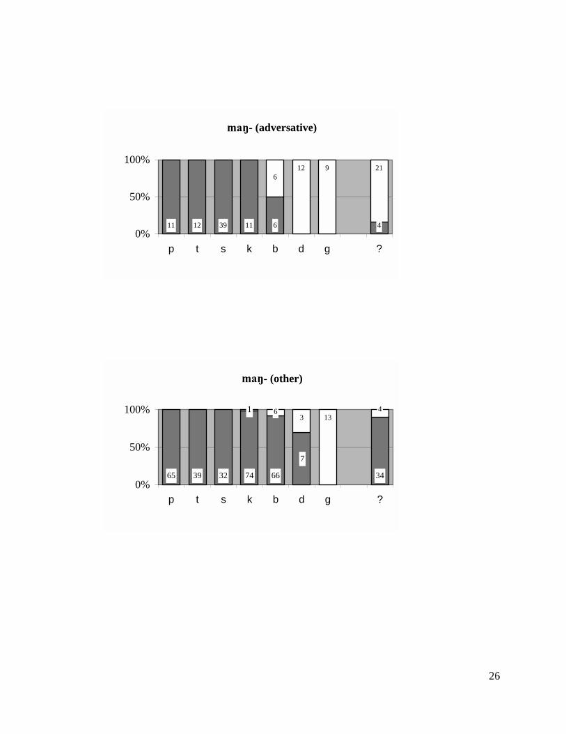
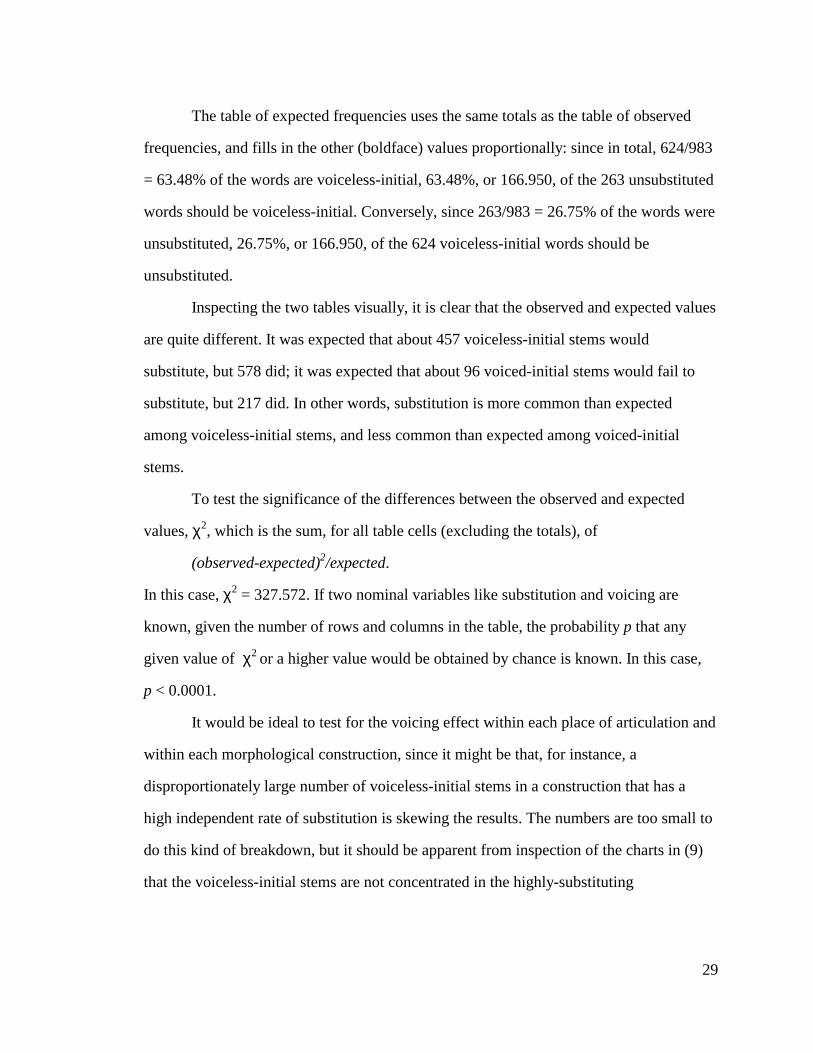
The constructions illustrated in (9) are adversative-verb-forming ���-;

nonadversative-verb-forming ���-; ���+RCV-, which forms mainly gerunds, but also

some less predictable nominalizations (������ ‘stitch’, pa-na- ����� ‘sewing’); ���+RCV-,

which forms professional or habitual nouns (������ ‘law’, mam-ba-������ ‘legislator’);

noun-forming ���- (instrumentals, gerunds, and unpredictable nominalizations, e.g.,

������ ‘expense’, ���-������ ‘spending money’); and reservative-adjective-forming ���-

(no other constructions had enough examples with each segment to make a chart

meaningful).

Within each chart, each obstruent is scaled for comparison. For example, the first

column in the first graph says that there are a total of 39 p-initial stems listed in English

(1986) that took the ���-RCV- construction, and of those, all are substituted. The fifth

column shows that there are 35 b-initial stems, of which 29 substitute, 1 varies, and 5 do

not substitute.

(� ��� � ‘tremble, thrill’, ��-� ��� � ‘to tremble, thrill’). There are no counterexamples to the second clause of the claim. De Guzman further claims that in instrumental adjectives, substitution is optional for voiceless Cs and impossible for voiced Cs and glottal stop. Instrumental adjectives are not included in (9) because there were too few tokens; there were indeed no substituted voiced Cs, but there were only 5 tokens of b, none of d, and 2 of g.

25

(9) Rates of substitution for various prefixes

���+RCV-

39 41 25 3 17

7 14 7

122 29

151

0%

20%

40%

60%

80%

100%

p t s k b d g ?stem-initial segment

Substituted Varies Unsubstituted

���+RCV-

18 25 20 7

12 12 6

1 119 15

3

20

1 2

0%

20%

40%60%

80%

100%

p t s k b d g ?

26

���- (adversative)

11 39 11 4

12 9 21

12 6

6

0%

50%

100%

p t s k b d g ?

���- (other)

65 32 74 34

3 134

6639

7

1 6

0%

50%

100%

p t s k b d g ?

27

���- (noun)

27 20 7 6

17 27 22

11251

51318

7

8

768

3

26

0%

20%

40%

60%

80%

100%

p t s k b d g ?

���- (reservative adjective)

3 2

7 4 5

211

33

3

17

3 5

55

0%

20%

40%

60%

80%

100%

p t s k b d g ?

28

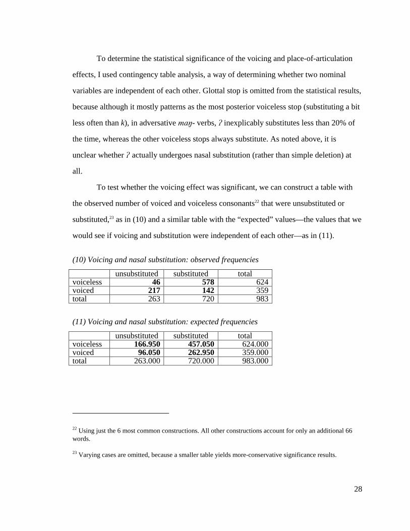
To determine the statistical significance of the voicing and place-of-articulation

effects, I used contingency table analysis, a way of determining whether two nominal

variables are independent of each other. Glottal stop is omitted from the statistical results,

because although it mostly patterns as the most posterior voiceless stop (substituting a bit

less often than k), in adversative ���- verbs, � inexplicably substitutes less than 20% of

the time, whereas the other voiceless stops always substitute. As noted above, it is

unclear whether ��actually undergoes nasal substitution (rather than simple deletion) at

all.

To test whether the voicing effect was significant, we can construct a table with

the observed number of voiced and voiceless consonants22 that were unsubstituted or

substituted,23 as in (10) and a similar table with the “expected” values—the values that we

would see if voicing and substitution were independent of each other—as in (11).

(10) Voicing and nasal substitution: observed frequencies

unsubstituted substituted total voiceless 46 578 624voiced 217 142 359total 263 720 983

(11) Voicing and nasal substitution: expected frequencies

unsubstituted substituted total voiceless 166.950 457.050 624.000voiced 96.050 262.950 359.000total 263.000 720.000 983.000

22 Using just the 6 most common constructions. All other constructions account for only an additional 66 words.

23 Varying cases are omitted, because a smaller table yields more-conservative significance results.

29

The table of expected frequencies uses the same totals as the table of observed

frequencies, and fills in the other (boldface) values proportionally: since in total, 624/983

= 63.48% of the words are voiceless-initial, 63.48%, or 166.950, of the 263 unsubstituted

words should be voiceless-initial. Conversely, since 263/983 = 26.75% of the words were

unsubstituted, 26.75%, or 166.950, of the 624 voiceless-initial words should be

unsubstituted.

Inspecting the two tables visually, it is clear that the observed and expected values

are quite different. It was expected that about 457 voiceless-initial stems would

substitute, but 578 did; it was expected that about 96 voiced-initial stems would fail to

substitute, but 217 did. In other words, substitution is more common than expected

among voiceless-initial stems, and less common than expected among voiced-initial

stems.

To test the significance of the differences between the observed and expected

values, χ2, which is the sum, for all table cells (excluding the totals), of

(observed-expected)2/expected.

In this case, χ2 = 327.572. If two nominal variables like substitution and voicing are

known, given the number of rows and columns in the table, the probability p that any

given value of χ2 or a higher value would be obtained by chance is known. In this case,

p < 0.0001.

It would be ideal to test for the voicing effect within each place of articulation and

within each morphological construction, since it might be that, for instance, a

disproportionately large number of voiceless-initial stems in a construction that has a

high independent rate of substitution is skewing the results. The numbers are too small to

do this kind of breakdown, but it should be apparent from inspection of the charts in (9)

that the voiceless-initial stems are not concentrated in the highly-substituting

30

constructions, and that within every construction, the voiceless-initial stems substitute

more frequently.

Similar contingency tables can be constructed for nasal substitution and place of

articulation. Here, we must break the data into voiceless and voiced cases, since we

already know that voicing has a strong effect, and the proportion of voiced- vs. voiceless-

initial stems is not steady across place of articulation. Observed and expected frequencies

are given in (12) and (13).

(12) Place of articulation and nasal substitution: observed frequencies

voiceless unsubstituted substituted total labial 6 163 169dental 25 276 301velar 15 139 154total 46 578 624

voiced unsubstituted substituted total labial 80 128 208dental 58 12 70velar 79 2 81total 217 142 359

(13) Place of articulation and nasal substitution: expected frequencies

voiceless unsubstituted substituted total labial 12.458 156.542 169.000dental 22.189 278.811 301.000velar 11.353 142.647 154.000total 46.000 578.000 624.000

voiced unsubstituted substituted total labial 125.727 82.273 208.000dental 42.312 27.688 70.000velar 48.961 32.039 81.000total 217.000 142.000 359.000

31

In (12) and (13), there are more rows, so trends are harder to spot. To make them

more apparent, (14) lists (observed-expected)/expected for each cell. A large negative

value means that the observed value was much lower than expected, and a large positive

value means that it was much higher than expected.

(14) Place of articulation and nasal substitution: (observed-expected)/expected values

voiceless unsubstituted substituted labial -0.518 0.041dental 0.127 -0.010velar 0.321 -0.026

voiced unsubstituted substituted labial -0.364 0.556dental 0.371 -0.567velar 0.614 -0.938

Recall that the place effect predicts that labials should be substituted more often

than expected (positive value in the top-right cell of (14)) and unsubstituted less often

than expected (negative value in the top-left cell), velars should be the opposite, and

dentals should fall somewhere in between. The tables in (14) show that in both the

voiceless and voiced cases, labials are substituted more often than expected (although the

effect is weak for voiceless p) and are unsubstituted less often than expected; velars are

substituted at about the expected rate when voiceless and much less often when voiced,

and are unsubstituted more often than expected in both cases. Dentals and velars can be

compared by noting that the tendency to be unsubstituted more often than expected is

greater than expected in velars than in dentals in both the voiceless (0.321 vs. 0.127) and

voiced (0.614 vs. 0.371) cases. In the voiced case, the tendency to be unsubstituted less

often that expected is much stronger among velars than among dentals (-0.935 vs. -

0.551); in the voiceless case, the difference between velars and dentals is tiny (although

in the right direction: -0.026 vs. -0.010)

32

We can perform a χ2 test for the place-of-articulation effect too, but the results are

less meaningful, because they tell us only that (12) and (13) are significantly different,

not whether the front-to-back trend is significant. The χ2 value for voiceless consonants is

5.264; for a table this size, the a probability of obtaining such a large χ2 by chance if

place of articulation and substitution were independent is p= 0.07. The χ2 value for

voiced consonants is 103.345, p < 0.0001. It is not surprising that the place differences

are small among the voiceless consonants, because in four of the six morphological

constructions included there is a ceiling effect—nearly all the voiceless consonants of any

place of articulation are substituted.

Finally, (15) summarizes the results of performing pairwise contingency-table

analyses between pairs of consonants. The test used was Fisher’s Exact Test,24 which

enumerates all tables having the same row and column totals as the table of observed

values. Each such table’s probability of occurring, assuming no association between the

variables (initial obstruent and nasal substitution), can be calculated. The probabilities for

the tables that are skewed in the same direction as the observed table, to the same degree

or more extremely, are added to find the probability p that such a skewed table could

have arisen by chance if the two variables were independent.

(15) Pairwise differences in rate of substitution

expected difference Fisher’s Exact Test p>b p < 0.0001 t,s>d p < 0.0001

voicing effect

k>g p < 0.0001 p>t p = 0.0528 t,s>k p = 0.6038 b>d p < 0.0001

place effect

d>g p = 0.0034

24 All statistical results were calculated in Statview.

33

2.2.3. Productivity of nasal substitution

There are several ways in which nasal substitution appears unproductive. First, despite

the lexical trends described above, it is of course not completely predictable which words

will undergo substitution—substitution is not even predictable among derivatives of the

same stem, as illustrated in (16). Note the lack of a strict implicational hierarchy for

substitution among the constructions ���-, ���+REDCV-, ���+REDCV-, and ���-.

(16) Differing behavior among derivatives of the same stem

������ ‘gift’ ��-������� ‘gifts to be distributed’ �-��-������� ‘act of giving away’ ����-��-������� ‘distributor’ ��-������� ‘to distribute (actor focus)’ � ����� ‘wallop’ �-�������� ‘wooden club used to pound clothes during washing’ ��-��-�������� ‘act of clubbing or pounding; assault’ ���-�������� ‘to wallop’ � ����� ‘harpoon’ �-������� ‘harpoon’ ���-��-������� ‘harpooner’ � ����� ‘whole’ ��-�� �� � ‘something used to produce a whole’ �-��-�� �� � ‘becoming whole; coagulation’ ��-�� �� � ‘to solidify; to clot’

Second, although the semantic connection between stem and derivative is always

apparent, exact meanings are sometimes unpredictable, especially with certain prefixes,

such as verbal ���-. Note that semantic idiosyncrasy is found in both substituted and

unsubstituted words:

34

(17) Semantic unpredictability with nasal-substituting affixes

����� ‘watcher’ ���- ����� ‘to wait near people who are eating, hoping to get

some food’ ������ � ‘woman’ ���-������ � ‘to have a mistress’ �� ��� ‘oppressed by a ruler’ ��-�� ��� ‘to strangle to death’ �������� ‘surface’ ���- �������� ‘veneer’�������� ‘visible’ ��-������ -��,���-���� -���25 ‘apparition, omen’ ��������� � � � � � � ‘water’ ��-������ ‘to urinate’ ������� � � � � � � ‘return’ �-������ ‘hand rudder’ ��������� � � � � � ‘hook’ ���-��-��������� ‘con man’

Third, certain affixes can cause unpredictable stress/length shifts. Note that this

idiosyncrasy too occurs in both substituted and unsubstituted words (but see (62)):

(18) Unpredictable stress/length shifts associated with nasal-substituting affixes

����� ‘sewing’ ���-��-������ ‘seamstress’ cf. ���� ‘remark’ � � ���-��-����� ‘critic’ ������ ‘town’ ���- �- ����� ‘resident of town’ cf. ������� ‘sickle’ � � ���-��-������� ‘person whose job it is to cut grass with a sickle’

25 This stem is exceptional: it has a final glottal stop only when suffixed.

35

������� ‘water’ ��-������� � � � � ‘to urinate’ cf. ������� ‘carpenter’s file’ � � ��-�������� � � ‘to chisel; to ask for money’ ������ ‘claws’ ��-����� ‘(type of) rat-trap’ �"#$� � ������� ‘weeding’ � � ��-������� ‘tool for weeding’

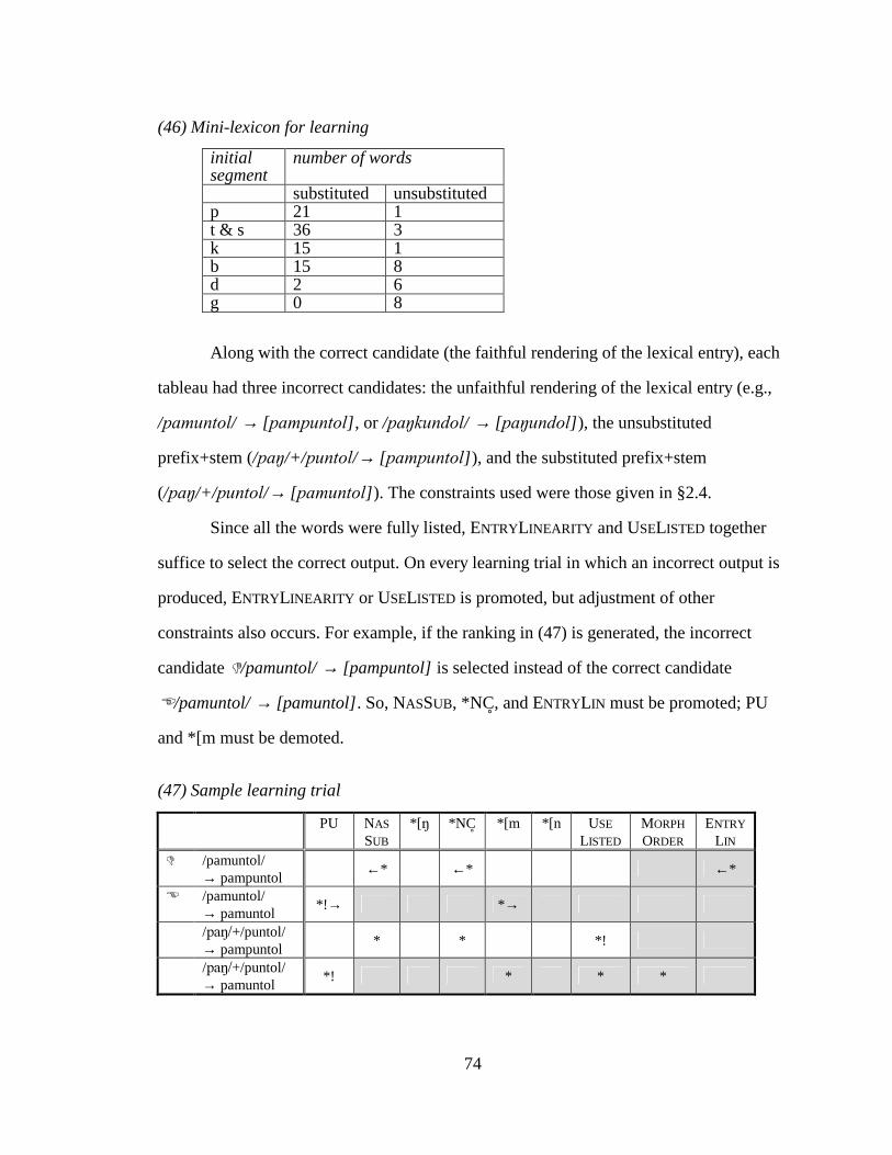
The result is that for many words with nasal-substituting affixes, a speaker must

know a number of facts not predictable from other words containing the same stem—

whether or not the word undergoes substitution, the meaning of the word, and the stress

of the word—and thus must maintain a separate lexical entry for that word (for a

discussion of other ways to encode the unpredictable information, see §2.5).

If most or all words with nasal substitution are fully listed, there is no need to

represent nasal substitution in the grammar: each word is simply pronounced the way it is

listed (see §1.1.1.1). The sticking point here is whether or not nasal substitution is part of

speakers’ competence. If it is, it should be accounted for (somehow). The following

section addresses this question experimentally.

36

2.3. An experiment

2.3.1. Introduction

I conducted an experiment aimed at answering two questions: (i) Is nasal substitution

productive? (ii) Are speakers aware of the lexical patterns within nasal substitution? If

the answer to either of these questions is yes, then perhaps nasal substitution belongs in

the grammar—certainly it must be accounted for somewhere in the system that governs

linguistic behavior, whether in the grammar or in some other subsystem. As discussed in

§1.3, this dissertation takes the approach that absent a clear understanding of how other

subsystems could account for a particular linguistic behavior, the behavior should be

accounted for by the grammar wherever plausible.

Nine native speakers of Tagalog living in Los Angeles participated. As shown in

(19), they ranged in age from 18 to 69, and had emigrated from the Philippines 3 to 20

years earlier (age at emigration did not correlate with productivity of nasal substitution).

(19) Personal characteristics of experiment participants

Participant # Age Age at emigration from Philippines 1 27 7 2 46 35 3 43 40 4 69 66 5 43 34 6 56 50 7 40 30 8 18 8 9 37 25

2.3.2. Task I: productivity

In the first task, participants were shown a series of cards, each of which had a

crude illustration of a person performing a farming or craft activity, with two sentences

37

(in regular Tagalog orthography, with accent marks26) printed at the top. A sample card is

shown in (20).

(20) Sample card for Task I

The sentences were designed as a “wug” test (Berko 1958) for the ���+RCV-

construction, which forms professional and habitual nouns (similarly to English -er):

participants had to produce the ���+RCV- form of a novel stem, which involved deciding

whether or not to perform nasal substitution. For example, in the sentence shown in (21),

the novel root is � ���, presented in a construction (���+RCV-) that does not permit

substitution. To fill in the blank, the participant would probably choose one of ���--

26 Accent marks—which are optional and not commonly used—indicate nonpenultimate stress and the presence or absence of final glottal stop. I used accent marks in this standard way, but also placed accent marks over penultimate stressed syllables, to ensure that the intended stress was always clear.

38

� ����(no substitution, no assimilation), ���--� ��� (assimilation only), or ��-

�-�� ��� (substitution).

(21) Sample sentence pair for Task I

Pagbubugnát ang trabaho niya. Siya ay ________________. to-bugnat (topic) job his/her He/she (inversion) His/her job is to bugnat. He/she is a ____________.

The experiment was carried out in individual sessions. Starting with two real-

word examples (blanks filled in) and then two real-word training items, the participant

took each card and read the sentences aloud, filling in the blank. Participants in Group A

(4 participants) were given some real words mixed in with novel words, and were told

that many of the words were rare and that if they didn’t know a word or its ���+RCV-

form, they should just guess. Participants in Group B (5 participants), were given only

novel words after the training items, and were told that the words were invented and there

were no right or wrong answers. (See §0 for a complete list of stimuli).

The purpose of the illustrations was to encourage participants to think of the

words as real. Since none of the participants grew up in a rural environment, it was

plausible that they would not be familiar with farming and craft terms. There is a large

part of the Tagalog vocabulary known as “deep Tagalog”—affixed words which have

been largely replaced by Spanish and English loanwords—so the idea that an unfamiliar

word could still be real and native should not seem too implausible to Tagalog speakers.

When Group A participants were told at the end of the experiment that most of the words

were in fact novel, three of the four expressed mild surprise; one said that he had so

suspected.

39

2.3.2.1. Results of Task I

The main result from Task I, shown in (22),27 was that substitution rates were much lower

than the rates found in the lexicon for ���+RCV-, but were higher than zero. In other

words, nasal substitution is neither very productive nor completely unproductive. Note

that Group B included one participant (#3, a Tagalog instructor at a university), who had

a very high rate of substitution. If she is omitted, the rate of substitution for Group B is

much lower. The difference between Groups A and B (A has a slightly higher

substitution rate) is not significant. To give some idea of the amount of inter-speaker

variation, (23) gives overall substitution rates for each participant; the four columns on

the left are speakers from Group A, and the five columns on the right are speakers from

Group B.

27 Token counts shown in (22) are for all speakers combined. Because Group A has one few speaker than Group B, token counts are not the same between the two groups. One token was omitted (from Speaker #3) because it could not be clearly classified as substituted or unsubstituted (���������� for �����—perhaps interference from ������ ‘literary work’, �����������‘author’?)

40

(22) Rates of substitution on novel words

Group A

4 3 4 53

8 9 8 79

15 11 11

1110%

20%

40%

60%

80%

100%

p t s k b d g ?

Substituted Unsubstituted

Group B

4 3 4 53 4

11 11 11 10

14 2012 11

10%

20%

40%

60%

80%

100%

p t s k b d g ?

41

(23) Overall rates of substitution on novel words, broken down by participant

Group B’s low rate of substitution (compared to the proportion of existing words

that substitute) is not surprising. This group was told they were dealing with novel words,

and it makes sense not to perform nasal substitution in coining a novel derived word, in

order to promote recoverability of the stem for the listener (especially since nasal

substitution neutralizes voicing and continuancy distinctions in the stem). With an

established word that would be familiar to the listener, recoverability is less of a concern.

The low rate of substitution for Group A might seem puzzling, though, because

this group was told they were dealing with real words, and so should be making guesses

that would match rates of substitution in the lexicon. But Group A was told they were

dealing with rare real words, and so they may still have been matching lexical

frequencies—the lexical frequencies found in rare words. Bloomfield (1917) asserted that

nasal substitution was more frequent among common words, and although I have no

0%

20%

40%

60%

80%

100%

1 4 5 9 2 3 6 7 8

Speaker #

substituted unsubstituted

Group A Group B

42

lexical-frequency data against which to test this assertion systematically, it seems

plausible.28

2.3.3. Task II: acceptability

The second experimental task was designed to determine whether or not participants’

grammars include the patterns of voicing and place of articulation seen in nasal

substitution. Substitution rates in the first task were too low to probe for effects of

voicing and place. Task II was administered immediately after Task I: starting with four

novel-word practice items (substituted and unsubstituted for each of two stems) each

participant (whether from Group A or Group B) was given cards with the same

illustrations and the same sentences as in Task I, but this time with the blanks filled in, as

shown in (24). Each root was presented twice (but not consecutively; order was

randomized), once substituted and once unsubstituted.

(24) Example stimuli for Task II

Kung pagbubugnát ang trabaho niya, siya ay mamumugnát. Kung pagbubugnát ang trabaho niya, siya ay mambubugnát. ‘If her/his job is to bugnat, she/he is a bugnat-er’

The participant read the sentences aloud, then stated his or her rating of the sentence pair,

on a scale from 1 (bad) to 10 (good).

2.3.3.1. Results of Task II

Participants’ acceptability judgments generally reflected lexical frequencies. (25) shows

the combined average for each segment of the rating given to a substituted stimulus

28 Cf. English verbs: irregulars tend to have higher frequency than regulars, in part because low-frequency irregulars are more likely to regularize over time (Bybee 1985).

43

minus the rating given to the corresponding unsubstituted stimulus. A positive number

means that over all, participants rated the substituted stimulus higher; a negative number

means that over all, participants rated the unsubstituted stimulus higher.

(25) Acceptability judgments: substituted - unsubstituted; error bars indicate 95%

confidence interval

The positive numbers for voiceless-initial roots and negative numbers for voiced-

initial roots mean that over all, participants tended to prefer the substituted stimuli for

voiceless-initial roots and tended to prefer the unsubstituted stimuli for the voiced-initial

roots, reflecting the voicing effect. And, except for the unexpectedly low ratings for p,29

acceptability judgments also reflected the place effect. The voiceless/voiced difference is

29 The p-t and p-s differences are not significant. I investigated the possibility that the low ratings for substituted p were the result of a neighborhood effect, but they do not appear to be: for each stimulus word, I counted the number of substituting and nonsubstituting words in its phonological neighborhood. The neighborhood was defined as the set of words sharing 5 segments, in the right positions (with empty codas counting as segments), with the target word. The average number of substituting words in the neighborhoods of the p stimuli was 2 (average number of unsubstituted = 0), and the average number of substituting words in the neighborhoods of the s and t stimuli was also 2 (average number of unsubstituted = 0.33).

-5

-4

-3

-2

-1

0

1

2

3

4

p t s k b d g ?

44

highly significant—p < 0.0001 by Scheffé’s F.30 The place effect is not very significant:

because of the low values for p-initial stems, the overall difference between bilabials and

dentals is not even in the right direction. The difference between bilabials and velars is in

the right direction, but is not significant (p < 0.0736 by Scheffé’s F). The difference

between dentals and velars is in the right direction and significant (p = 0.0168 by

Scheffé’s F).

An ANOVA on voicing, place, and speaker shows that there was no significant

interaction between voicing and place, meaning that the magnitude of the voicing effect

does not vary significantly by place of articulation, and the magnitude of the place effect,

such as it is, does not vary significantly by voicing. There were, however, significant

interactions between voicing and speaker (F = 3.088, p = 0.0056) and between place and

speaker (F = 3.402, p = 0.0002), meaning that the voicing and place effects had different

strengths for different speakers. There was no significant difference in acceptability

ratings between Group A and Group B.

30 For the ANOVA and Scheffé’s results, some data had to be omitted into order to balance cells. Data for s-initial stems were omitted (to avoid having twice as many data points for voiceless dentals as for other categories); data for one of the da-initial stems was omitted (to avoid have 25% more data points for d than for other segments); and data were excluded for participant #6, who made several errors in reading aloud the stimuli (not applying substitution, although the stimulus was substituted; the errors were all on velar-initial stems, which can be confusing to read because the digraph “ng” is used to represent �).

45

2.4. The grammar

2.4.1. Desiderata for an analysis

The experimental results described above suggest that nasal substitution and its patterns

must be modeled in the grammar, in a way that accounts for the following facts: existing

words with nasal-substituting affixes are listed; speakers rarely perform nasal substitution

on novel words or rare words; and listeners prefer nasal substitution on voiceless

obstruents over voiced, and front over back.

The basic model that I will propose involves high-ranking input-output

correspondence constraints that cause established words to be pronounced as listed, with

lower-ranked markedness constraints that come into play when no listed form is available

(as with a novel word). This section presents the constraints involved in nasal

substitution, and shows how they interact to produce novel utterances and to produce

utterances based on listed words. Subsequent sections show that the grammar proposed is

learnable from the lexical data, that the grammar predicts appropriate behavior by both

speakers and listeners, and that the interaction of speakers and listeners maintains lexical

patterns.

2.4.2. Paradigm Uniformity

Paradigm Uniformity, also known as Output-Output Correspondence, enforces similarity

among related words (Crosswhite 1996 and 1998, Steriade 1996, Kenstowicz 1997,

Benua 1998). For any word, there are potentially many other words to which it could be

seen as related: ��-������ is clearly related to the bare-stem word �����, perhaps related

to other derivatives of the stem �����, and perhaps even related to other words with the

prefix ���-. It is clear that nasal substitution reduces similarity between the nasal-

46

substituted word and unsubstituted derivatives of the same stem, including the bare stem,

violating Output-Output Correspondence constraints. I will use PU as a shorthand for

those correspondence constraints that enforce similarity between an unsubstituted stem

like ����� and the substituted form of that stem found in ��-������ and are violated by

nasal substitution (e.g., IDENT-OO[SONORANT], IDENT-OO[VOICE] for voiceless-initial

stems). Candidates with nasal substitution violate PU once, and candidates without nasal

substitution do not violate PU.

2.4.3. Input-Output Correspondence

PU is one of the forces that discourage substitution in novel words. Input-Output

Correspondence is part of the force that allows substitution in words that are listed as

substituted (USELISTED, discussed below, is the other crucial part).

Input-Output Correspondence enforces similarity between an input and an output,

and thus encourages substitution if the input is a substituted word, but discourages

substitution if the input is an unsubstituted word or a prefix+stem combination. Adopting

the view of Lapoliwa (1981), Newman (1984), and Pater (1996), nasal substitution is a

coalescence of two segments, as illustrated in (26).

(26) Nasal substitution as coalescence

% �1 �2 �3/ + / �4 �5 �6 �7 �8 /

[ �1 �2 �3,4 �5 �6 �7 �8 &�

Matching subscripts indicate that a segment in the output is the correspondent of a

segment in the input, so /���3/+/4����/ → [���3,4����] means that the surface segment

[�3,4] corresponds to both the input segment /�3/ and the input segment /4/. The

47

coalescence analysis allows output [�3,4] to straightforwardly inherit some of the features

of /�3/ (manner features) and some of the features of /4/ (place features). If one of the

input segments were actually deleted, the analysis would be more complicated, requiring

constraints that preserve the features of an input segment even if that segment is not

present in the output.

Coalescence can produce featural misidentity between the prefix nasal and the

coalesced nasal—/�3/ is [dorsal], but [�3,4] is [labial]—and between the underlying stem-

initial obstruent and the coalesced nasal—/4/ is [-sonorant], but [�3,4] is [+sonorant];

thus, nasal substitution violates IDENT-IO constraints. Coalescence also alters the

precedence relations between segments in the underlying string: in the input, segment 3

strictly precedes segment 4, but in the output, it does not.

There is a difference, though, between substitution of a synthesized prefix+stem

combination and substitution of an unsubstituted listed word (if that listed word is a

phoneme string—see §2.5 for consideration of other possibilities). In /���3/+/4����/ →

[���3,4����], the precedence relation that is interrupted is between segments that do not

belong to the same lexical entry (/�3/ and /4/); within the prefix and within the stem, all

precedence relations are preserved. If coalescence applies to a single listed word,

however, as in /���34����/ → [���3,4����], however, the precedence relation that is

disturbed is between two members of the same lexical entry. Pater (1996) differentiates

between LINEARITY, which is violated by any coalescence, and ROOTLINEARITY, which is

violated only by coalescence within a root. I will instead make the distinction between

MORPHORDER, which is violated by disturbing the linear order of morphemes (such as by

coalescing members of two different morphemes) and ENTRYLINEARITY, which is

violated by disturbing the linear order of segments (as by coalescence) within a lexical

entry coalescence:

48

(27) Constraints against coalescence

MORPHORDER

If morpheme µ1 precedes µ2 in the input, then all the segments of µ1 must precede all the segments of µ2 in the output.

ENTRYLINEARITY

If segment X precedes segment Y within a lexical entry, A is the output correspondent of X, and B is the output correspondent of Y, then A must precede B.

Pater justifies ROOTLINEARITY by the fact that roots often contain a richer

contrast set than affixes, but it could also be seen as justified by work such as Cho (to

appear), which suggests that timing relations between gestures belonging to different

morphemes are much more variable than timing relations between gestures belonging to

the same morpheme, implying that violating timing relations such as precedence within a

lexical entry is more strongly avoided than violating timing relations across lexical

entries.

The table in (28) summarizes the role of Input-Output Correspondence in nasal

substitution by showing the CORR-IO31 violations of a variety of input-output pairs.

31 “CORR-XY” stands for any constraint affecting correspondence between X and Y (IDENT[F]-XY, MAX-XY, DEP-XY, etc.)

49

(28) Corr-IO constraints: sample violations

‘to � ���j’ IDENT [PLACE]

IDENT [SON]

DEP MAX MORPH ORDER

ENTRY LINEARITY

/�����3/+/�4��/ → [���3,4��]� * * *

/���3/+/�4��/ → [���3��] * * /���3/+/�4��/ → [���4��] * * /���3/+/�4��/ → [���3b4��]� * /���3�4�/ → [���3�4�]� /���3�4�/ → [���3b�4�]� * /���3�4�/ → [���3b3�4�]� * *32 /���3b4��/ → [���3,4��]� * * /���3b4��/ → [���3��] * /���3b4��/ → [���4��] * * /���3b4��/ → [���3b4��]�

2.4.4. Listedness

This section introduces a constraint USELISTED, which requires that a single lexical entry

be used as input (rather than a prefix+stem combination). If no such entry is available,

USELISTED is irrelevant, because it is violated by all candidates, but if such an entry is

available, USELISTED requires that it be used.

It is usually assumed that the input to a tableau is a particular lexical entry or

combination of lexical entries; CORR-IO constraints evaluate each output candidate’s

faithfulness to that one input. I will assume instead (as in (28)) that each candidate is an

input-output pair—different candidates can have different inputs—and CORR-IO

constraints evaluate correspondence within each pair. The real “input” to a tableau that is

shared by all candidates is the morphosyntactic and semantic features that the speaker

wishes to express, which I will call the intent; there may be more than one lexical item or

combination of lexical items that could express that intent. This means that Gen, the

component of the grammar that generates the candidate set, must generate a complete set

32 “Splitting” a segment can be thought of as a violation of ENTRYLINEARITY, because in the input, segment 3 does not precede itself, but in the output, it does.

50

of outputs for each input that is available in a given tableau. As in (28), two distinct

candidates may share the same33 output, but have different inputs.

USELISTED enforces a preference for candidates whose inputs consist of a single

lexical entry, rather than a string of morphemes:

(29) USELISTED

The input portion of a candidate must be a single lexical entry. (1 violation if not true)34

The tableaux in (30) illustrate the operation of USELISTED. I assume that high-

ranked constraints enforce morphosyntactic and semantic identity between intent and

output, preventing some unrelated lexical entry or prefix+stem combination from being

used.35 In (30), these constraints are included in the shorthand constraint MEANING, which

I omit from subsequent tableaux. In the first tableau, candidate a, which uses a single

lexical entry, satisfies both MEANING and USELISTED. Candidate b satisfies MEANING,36

but violates USELISTED, because it uses a combination of two lexical entries. Candidate c

33 The outputs are not exactly the same, because their segments are in correspondence with the segments of different inputs.

34 It might be desirable to make USELISTED sensitive to the number of lexical entries beyond a binary one/many opposition (i.e., preferring a candidate that uses a lexicalized prefix-stem combination plus a suffix over a candidate that concatenates prefix+root+suffix afresh), but the constraint as defined will suffice for present purposes.

35 Or perhaps the restriction is in GEN (the function that generates the set of candidates) itself. Using high-ranking constraints instead is attractive, though, because it allows speech errors in which the wrong input is (e.g., deviant for devious) to be described as the result of very rare rankings (see §2.4.7).

36 A prefix+stem combination does not completely satisfy MEANING when the meaning of the existing single lexical entry is idiosyncratic but it satisfies what would presumably be the highest-ranking MEANING constraints. For example, if a speaker wants to talk about a rudder (for which there is a listed word,, /pamalik/ ‘rudder’), her linguistic intent is not perfectly satisfied if she synthesizes /pa��+/balik/ (however she decides to pronounce it), which should mean just ‘tool for returning’. But /pa��+/balik/ would satisfy her intent better than an input that lacked the meaning ‘tool’, or was not a noun, or meant ‘tool for digging’.

51

uses a single lexical entry, but it violates MEANING, because it is not Actor-Focus (it is

Patient-Focus). Candidate d violates MEANING because it is [-distributive] (it would

simply mean ‘to give’). In the second tableau, bugnat is a novel stem, and so there is no

lexical entry /mamugnat/ available, and all possible candidates violate USELISTED.

(30) Violations of USELISTED

Intent: V, Actor-Focus ‘to distribute’ MEANING USELISTED (a) /mamigaj/ → [mamigaj] (b) /ma�/+/bigaj/ → [mamigaj] * (c) /�ipamigaj/ → [�ipamigaj] * (d) /mag/+/bigaj/ → [magbigaj] * *

Intent: V, Actor-Focus ‘to bugnat’ MEANING USELISTED (e) /ma�/+/bugnat/ → [mamugnat] * (f) /mag/+/bugnat/ → [magbugnat] * *

Are all lexical entries equally available? Surely the leap during word-learning

from unknown word to fully available lexical entry is not instantaneous. More-frequent

words seem to have stronger lexical entries—they are, for example, faster to recognize

(Rubenstein, Garfield, & Millikan 1970; Forster & Chambers 1973). Frisch (to appear)

reports experimental results in which subjects who were exposed to a novel word twice

rated it more “word-like” than subjects who were exposed to a novel word just once,

suggesting that a word is not immediately accepted the first time it is heard. The model

here assumes that rather than simply being listed in the mental lexicon or not, lexical

entries range in strength from 0 (not at all listed) to 1 (always available for use). Strength

of a lexical entry in this model is a function of the number of times a speaker has heard

the word, although in real life there are probably other factors, such as who the speaker

has heard the word from and in what context.

52

There are two ways of implementing “gradient listedness” in the grammar. One is

to replace USELISTED with a family of inherently ranked constraints such as

USE100%LISTED >> USE90%LISTED >> ... >> USE10%LISTED >> USELISTED

where USEX%LISTED is satisfied by a candidate whose input lexical entry is X% listed or

more. Other constraints could be inserted into this hierarchy. For example, if

USE40%LISTED >> PU >> USE30%LISTED

a nasal-substituted derivative with 30% listedness (i.e., of whose listedness the speaker is

30% certain, or whose lexical entry’s strength is 30% of the maximum possible strength)

or lower will not be used because Paradigm Uniformity to the base forbids nasal

substitution. But a nasal-substituted derivative with 40% listedness (or higher) would

override PU and be used. This is illustrated schematically in (31): Candidate a, the

faithful parse of the single lexical entry, fails because it violates PU; candidate b satisfies

PU, but violates CORR-IO. Candidate d is the optimal candidate because, although it

violates USE30%LISTED, it satisfies PU, which is more highly ranked. But in the second

half of the tableau, candidates are available that satisfy USE40%LISTED, and so candidate

(e) is optimal despite its violation of PU.

(31) Interaction of a family of USEX%LISTED constraints and Paradigm Uniformity

ENTRY LINEARITY

USE40% LISTED

PU USE30% LISTED

(a) ��� �����(30% listed) → [�� ���� * *! (b) /manala/ (30% listed) → [�� ����� *! * (c) ����/+/tala/ → [�� ���� * *! * (d) � ����/+/tala/ → [�� ����� * * (e) � /�� ���� (40% listed) → [�� ���� * (f) /�� ���� (40% listed) → [�� ����� *! (g) ����/+/sili/ → [�� ���� *! * * (h) ����/+/sili/ → [�� ����� *! *

53

The other way to approach gradient listedness is to have a single constraint,

USELISTED, with the availability of a given lexical entry in any utterance equal to the

listedness of the entry. For example, a word that is 30% listed has a 30% probability of

being available in any given tableau. The ranking CORR-IO, USELISTED >> PU produces

the result ��� �����→ [�� �����30% of the time (upper tableau in (32)—listed /manala/

is available as an input), and the result ����/+/tala/ → [�� ����� 70% of the time

(lower tableau in (32)—synthesized candidates only).

(32) Interaction of a unitary USELISTED constraint and Paradigm Uniformity

ENTRY LINEARITY

USE LISTED

PU

(a) � ��� �����→ [�� ���� * (b) /manala/ → [�� ����� *! (c) �����+�tala/ → [�� ���� *! * (d) �����+�tala/ → [�� ����� *! (g) �����+�tala/ → [�� ���� * *! (h) � �����+�tala/ → [�� ����� *

In contrast, we would see ��� �����→ [�� �����40% of the time, and ����%+%tili/

→ [�� ����� 60% of the time. This may seem like an obvious empirical difference

between the unitary-USELISTED approach and the USEX%LISTED approach, which

produced uniformly ��� �����→ [�� �����and uniformly ��� �����→ [�� ���� in (31),

but under the stochastic constraint ranking scheme introduced below, the difference is not

so clear. For that reason, I will use unitary USELISTED.

2.4.5. Constraints specific to nasal substitution

Nasal substitution is some 5000 years old (see fn. 83). The original phonetic motivation

might have been consonant-cluster avoidance, as suggested in Archangeli, Moll, and

Ohno 1998; post-nasal lenition; or an attempt to avoid a non-crisp edge (prefix nasal and

stem-initial consonant sharing place of articulation, as required by nasal assimilation), as

54

suggested in Pater 1999b. I suspect that modern Tagalog nasal substitution is divorced

from any phonetic or prosodic motivations, and simply exists as an arbitrary alternation.37

Accordingly, I will propose a constraint, NASSUB (short for “nasal-substitute”) that

simply requires nasal substitution:

(33) NASSUB38

* W µ µ | | X X | | [+nasal] [-sonorant] A morpheme-final nasal must not be immediately followed by an obstruent within the same word. 39

I will assume that NASSUB penalizes failure to substitute in both synthesized

prefix+stem candidates, and in candidates whose input is a single listed word.40 This is

because even although a morphologically complex lexical entry like /mami�aj/ contains

no morpheme boundaries, its segments are coindexed to related lexical entries: the first

37 Note that the prefixes mag- and pag- also produce consonant clusters—and, with velar-initial stems, non-crisp edges (e.g., mag-� �� ���-an ‘to appraise each other’ from � ������, � ���� � ‘carat’), unless some mechanism requires the g and k to have separate-but-identical features. But these prefixes do not induce coalescence, even though the identity violations would be no worse those incurred in nasal substitution.

38 Representations in constraint definitions should be interpreted as nonexhaustive at the edge of each tier. For example, in (33), other morphemes may come before or after the two shown, but not between. When tiers are missing, the information on those tiers should be considered irrelevant. For example, in (34), the two segments may belong to different morphemes or to the same morpheme.

39 Where “word” must be defined so as to exclude the compounding-like prefixes discussed in fn. 14, which never trigger nasal substitution.

40 Although this assumption is not crucial to the model proposed here—once a word is listed as unsubstituted, ENTRYLINEARITY almost always prevent NASSUB from having any effect.

55

three segments (mam) are coindexed with the segments of the lexical entry for the prefix

/ma�-/, and the last five segments (mi�aj) are coindexed to the segments of the lexical

entry for the word /b��aj/. The candidate /mami�aj/ → [mami�aj] satisfies NASSUB,

because there is no sequence of a distinct nasal and obstruent coindexed to two different

morphemes.

Turning to the constraints that produce the patterns in the lexical distribution of

nasal substitution,41 I attribute the higher rate of substitution on voiceless-initial stems to

a constraint *NC �, a constraint forbidding a sequence of a nasal and a voiceless obstruent:

(34) *NC �

* W X X | | [+nasal] [-voice, -sonorant] A [+nasal] segment must not be immediately followed by a [-voice, -sonorant] segment within the same word.

Hayes and Stivers (1996) give a phonetic motivation for *NC �: the raising of the

velum during the nasal-to-oral transition expands the oral cavity, slowing the buildup of

the supraglottal air pressure that would otherwise “turn off” voicing. An NC � sequence

thus requires extra effort (such as glottal abduction) to keep the obstruent voiceless.

41 This is a form of Emergence of the Unmarked (McCarthy & Prince 1994): although nasal substitution itself is not motivated by pure markedness, the patterns in its distribution seem to reflect considerations of markedness.

Newman (1984) finds an implicational hierarchy reflecting similar effects in related languages in which nasal substitution is predictable if the stem-initial obstruent is known: If the language substitutes g, it also substitutes d, and if a language substitutes d, it substitutes b; similarly, substitution on k implies

56

Hayes and Stivers propose that the articulatory difficulty of NC � clusters drives postnasal

voicing. Pater (1996) discusses *NC � as the motivation for postnasal voicing, Indonesian

nasal substitution (which applies only to voiceless obstruents), nasal deletion,

and denasalization.42

*NC � favors substitution in voiceless-initial stems. A word like mantukad, without

substitution, violates *NC �, but manukad, with substitution, does not. *NC � is irrelevant for

voiced-initial stems, since it is violated by neither substitution (mandukad) nor

nonsubstitution (manukad).

If *NC � is ranked high enough to produce an effect in nasal substitution, why is

*NC � violated so freely word-internally? One answer is the distinction made above

between MORPHORDER and ENTRYLINEARITY:

(35) Coalescence within vs. across listed items

/���1�+��2���/ ENTRY LINEARITY

*NC� MORPH ORDER

�����1,2��� * ���1�2��� *! /�� 1�2���/ ��� 1,2��� *!

���� 1�2���� *

substitution on t,s and p. In addition, substitution on b implies substitution on p, d on t,s, and g on k. Thanks to Joe Pater for pointing out this interesting finding.

42 Pater 1999b proposes instead that Alignment is the driving force behind Indonesian nasal substitution, and that IDENT-IO for pharyngeal expansion (see Steriade 1995) is what restricts nasal substitution to voiceless obstruents: voiced obstruents require pharyngeal expansion to maintain transglottal airflow despite a vocal tract obstruction, and so are [+pharyngeal expansion], but voiceless obstruents—which lack transglottal airflow—and nasals—which lack a vocal-tract obstruction—are [-pharyngeal expansion]. So, fusing a voiced obstruent and a nasal violates IDENT[PHARYNGEAL EXPANSION], but fusing a voiceless obstruent and a nasal does not. This approach might work for Tagalog as well (with stochastic constraint ranking).

57

If ENTRYLINEARITY is very highly ranked, *NC� will not be able to shape the

lexicon root-internally the way it seems to have done for nasal substitution (by a

mechanism proposed below).43

To introduce the constraints that produce the place-of-articulation effect, consider

the chart in (36), showing the distribution of various consonants in various positions

within the root in Tagalog. The numbers are from a database of about 4,600 disyllabic

Tagalog roots,44 with reduplicated roots excluded.

43 But see fn. 42: adopting Pater’s (1999b) approach to Indonesian, the voicing effect would be driven by a difference in faithfulness (rather than a difference in markedness), in which case there is no drive to coalesce nasal-obstruent clusters word-internally. Under the learning mechanism discussed below, though, there is no way to prevent *NC� from being learned with a fairly high ranking, so we would still have to rely on ENTRYLINEARITY to prevent root-internal coalescence.

44 All the native, disyllabic roots in English 1986 were recorded. The count shown is by type—each root is counted just once, no matter how many affixed forms it has. The restriction to disyllabic roots is necessary because monosyllables are clitics (pronominal and discourse), which may not obey the same morpheme structure constraints as lexical roots, and roots of more than two syllables are—at least historically—polymorphemic. Because of evidence that speakers may treat words that appear polymorphemic as polymorphemic, even without morphosyntactic motivation (see Baroni 1998, Hammond 1999, and Chapter 4 of this dissertation), words with more than two syllables might therefore also escape root structure constraints.

58

(36) Distribution of consonants in roots of the form C1V(C2)C3V(C4)

354503

463

321

452

218

16773

32 46

522

52 32

496

275

31

14741

159

165

307

368245

301

335

253 247

172

227

159

614

236 197

174

178

98

421 353 355

59

201265

61

184

383

258

234 169575

39

50

19266

9

264

27

0%

10%

20%

30%

40%

50%

60%

70%

80%

90%

100%

p t s k b d/r g m n N l j w ? h

C1 C2 C3 C4

59

Note that in general, fronter consonants are better represented root-initially.45 For

example, about 45% of ps are root-initial (C1), but only about 28% of ks are root-initial.

Note further that obstruents are better represented initially than are sonorants. There are

very few root-initial nasals, both over all and as a proportion of nasals in all positions;

among the nasals, m is better represented root-initially than n or �. This consonantal

distribution suggests that (and would provide evidence to the learner that) root-initial

nasals are disfavored, but that among the root-initial nasals, the fronter ones are less

disfavored.

I propose the following family of constraints against root-initial nasals: *[root�,

*[rootn, *[rootm (abbreviated *[�, *[n, *[m).

(37) *[�, *[n, *[m

* [root X [root X [root X | | | [+nasal, +dorsal] [+nasal, +coronal] [+nasal, +labial] A root must not begin with [�] ([n], [m]).

This family of constraints disfavors substitution.46 For example, ma-nukad, with

substitution, violates *[n, because the n that results from substitution is root-initial (as

well as prefix-final). But man-tukad, without substitution, does not violate *[n], because

the n belongs to the prefix only. The ranking *[� >> *[n >> *[m (which could be inherent

45 Ingram (1974) proposes “fronting” as an acquisition strategy: a front-to-back order is preferred for both consonants and vowels within a word (i.e., ...p...t..., ...p...k..., and ...t...k... are preferred to ...t...p..., ...k...p..., or ...k...t...; ...i...u... is preferred to ...u...i...).

46 in synthetic candidates as well as in candidates with single-lexical-entry inputs, because the n in a lexical entry /manukad/ would be coindexed to the t of the related word /tukad/. This assumption does not materially affect the model presented here, however (see fn. 40).

60

or learned) would disfavor substitution most on posterior places of articulation.47 For

example, if *[� >> *[n >> NASSUB >> *[m, then all else being equal, substitution would

occur on a labial-initial root, but not on a coronal- or velar- initial root:

(38) *[� >> *[n >> *[m

/����+�bala/ *[� *[n NASSUB *[m (a) � mamala * (b) mambala *!

/����+�dala/ (c) � mandala *! (d) manala *

/����+�gala/ (e) � maNgala *! (f) maNala *

Is there any functional motivation for dispreferring root-initial nasals, or for

especially dispreferring root-initial back nasals? Among voiceless obstruents, the place

effect could be seen as a fine-tuned version of *NC�. Recall that the phonetic motivation

proposed by Hayes and Stivers (1996) for *NC � is that the expansion of the oral cavity

during velum-raising encourages voicing. Their model also found that frontness of the

obstruent encourages voicing, because there is a greater expanse of flexible cheek wall

that can expand outward and reduce supralaryngeal pressure. This would explain why p

substitutes more often than k. But it does not explain why b substitutes more often than d,

since turning off voicing is not necessary in mb, nd, and �� clusters—indeed, the

frontness of b would make voicing easier to maintain, 48 and thus the cluster mb would be

less marked (and so less subject to repair by coalescence) than nd or ��.

47 Cf. English, in which root-initial � is not permitted at all.

48 See Ohala & Riordan (1980), who found that passive cavity expansion maintained voicing longer for b than for d or g.

61

Another possibility, expanding on Pater 1999b (see fn. 42), is that IDENT-IO

violations are greater when substituting a fronter consonant. Pater proposes that the

reason voiced obstruents do not substitute in Indonesian is that if they did, it would

violate IDENT-IO[PHARYNGEAL EXPANSION]: voiced obstruents are [+pharyngeal

expansion]—they require active expansion of the pharynx, or some other exertion, to

maintain voicing—but nasals are [-pharyngeal expansion], because voicing is maintained

by venting air out the nose. Fronter consonants should require less pharyngeal expansion,

because more cheek area is available for passive expansion, and so coalescing a b with a

nasal is less of a violation of (some gradient version of) IDENT-IO[PHARYNGEAL

EXPANSION]. The place effect among voiceless consonants is then a puzzle, though,

because no voiceless consonants require any pharyngeal expansion.

Whatever the reason, the Tagalog lexicon manifests a dispreference for root-

initial nasals, so I will simply assume the *[NASAL constraint family. Although there may

be a reason for the family to be inherently ranked *[� >> *[n >> *[m, this ranking is

learnable from the lexicon (see §2.6), so it need not be assumed.

2.4.6. Summary of constraints

The table in (39) summarizes the constraints relevant to determining whether a word is

pronounced with nasal substitution.

62

(39) Constraints affecting nasal substitution

Constraint Effect PARADIGM UNIFORMITY discourages N.S. (nasal substitution) NASSUB encourages N.S. *NC � encourages N.S. for voiceless-initial stems *[� discourages N.S. for velar-initial stems *[� discourages N.S. for coronal-initial stems *[� discourages N.S. for bilabial-initial stems MORPHORDER discourages N.S. in prefix+stem concatenations ENTRYLINEARITY encourages N.S. if word is listed with substitution

discourages N.S. if word is listed without substitution.

As noted above, if a word has a listed form, and it is available, and

ENTRYLINEARITY is ranked high, the word will be pronounced as listed:49

(40) Input-Output Correspondence requires use of listed form

ENTRY LIN

USE LISTED

*[� *NC� *[n NAS SUB

PU MORPH ORDER

*[m

(a) � /����������/ → ����������

*

(b) /����������/ → ���������

*! * *

(c) /����+��������/ → ����������

*! *

(d) /����+��������/ → ���������

*! * * *

ENTRY

LIN USE

LISTED *[� *NC� *[n NAS

SUB PU MORPH

ORDER *[m

(e) � /��������/ → ��������

* *

(f) /��������/ → ���������

*! *

(g) /����+�b�����/ → �������

*! * * *

(h) /����+�b�����/ → ���������

*! *

49 Candidate f in (40) results from splitting underlying m into m and b. Epenthesizing the b instead would produce a homophonous candidate (not shown) that satisfies ENTRYLINEARITY but violates high-ranking DEP.

63

But when no listed form is available, as in a novel word, ENTRYLINEARITY is

satisfied by all candidates, and USELISTED cannot be satisfied by any candidate, so both

are irrelevant; the lower-ranked constraints decide. The tableau in (41) illustrates how the

constraint ranking in (40) would treat a novel root beginning with each obstruent.

(41) Coining of novel words, using the ranking in (40)

���- form of /����/

ENTRY LIN

USE LISTED

*[� *NC� *[n NAS SUB

PU MORPH ORDER

*[m

(a) � /ma��+�pala/ → ������

* * * *

(b) /ma��+�pala/ → �������

* *! *

(c) � /ma��+�tala/ → �� ���

* * * *

(d) /ma��+�tala/ → �� ����

* *! *

(e) � /ma��+�sala/ → �� ���

* * * *

(f) /ma��+�sala/ → �� ����

* *! *

(g) � /ma��+�kala/ → �������

* * *

(h) /ma��+�kala/ → ������

* *! * *

(i) � /ma��+�bala/ → ������

* * * *

(j) /ma��+�bala/ → �������

* *!

(k) � /ma��+�dala/ → �� ����

* *

(l) /ma��+�dala/ → �� ���

* *! * *

(m) � /ma��+�gala/ → ������

* *

(n) /ma��+�gala/ → ������

* *! * *

Under this ranking, in which PU is fairly low, the ranking of *NC � with respect to

the three anti-root-initial-nasal constraints (*[�, *[n, *[m) creates a place-of-articulation

cutoff among the voiceless obstruents; in this case, labials and coronals substitute, and

64

dorsals do not. The ranking of NASSUB with respect to the three nasal constraints places a

cutoff among the voiced obstruents; in this case, only labials substitute.

2.4.7. Stochastic constraint ranking

Of course, this cannot be the constraint ranking for the language, because not all novel b-

initial stems (for example) were substituted in the experiment. There is no one ranking

that would be compatible with the experimental results above on novel stems, because for

every consonant tested, there were some tokens in which speakers substituted it, and

some in which they did not.

For this reason, I will adopt stochastic constraint ranking, as proposed in Hayes

and MacEachern 1998, Boersma 1998, Boersma and Hayes 1999, and Hayes (to appear).

Stochastic constraint ranking is similar to variable constraint ranking (as in Anttila 1997).

In Anttila’s system, certain ranking pairs within a hierarchy are fixed, and all ranking

permutations of the constraints that respect those fixed pairs are equally possible. For

example, with constraints C1, C2, C3, and C4 and the ranking C1 >> {C2, C3} >> C4, there

is a 50% probability of speaker’s using the ranking C1 >> C2 >> C3 >> C4 in any given

utterance, and a 50% probability of using C1 >> C3 >> C2 >> C4.

Stochastic constraint ranking differs from variable constraint ranking in that rather

than having only two types of ranking between any two constraints (completely fixed and

completely free), any ranking is possible, but some are more probable than others. This is

implemented by assigning each constraint a probability distribution centered on a

particular ranking value. In any given utterance, an actual value is generated for each

constraint, at random but in accordance with the constraint’s probability distribution.50

50 And, in Boersma’s system, using a quantity called “ranking spread”. Full details are given below, in “The Speaker”.

65

The dominance relations in the constraint hierarchy are determined by these actual

values. For example, consider the hypothetical constraint system in (42). C1 has a fairly

high ranking value, C2 and C3 are somewhat lower, and C4 is quite a bit lower.

(42) Hypothetical constraint system

In nearly all of the linear rankings that would be produced by this system on

various occasions, C1 outranks the other three constraints, because its distribution is

centered on a much higher ranking value. This means that it would be possible, but

vanishingly unlikely,51 for C1 to be ranked low enough, and/or any other constraint to be

ranked high enough, for C1 to be dominated. Similarly, it is very improbable that C4 will

outrank any other constraint. But C2 and C3 overlap considerably, which means that their

ranking with respect to each other varies quite a bit. This system is different, however,

from an Anttila-style C1 >> {C2, C3} >> C4 system in that it encodes a weak tendency for

C2 to outrank C3 rather than completely free ranking between the two.

Stochastic constraint ranking allows us to model a situation in which nasal

substitution rarely occurs in any novel word, but it is more likely to occur on a voiceless-

51 See §2.7 for calculations of probability.

C1 C2 C3 C4

high ranking low ranking

prob

abili

ty d

ensit

y

66

or front-initial stem: PU and MORPHORDER will tend to prevent substitution, but

substitution will occur on a voiced-initial segment whenever NASSUB outranks PU and

the relevant *[NASAL constraint, and on a voiceless-initial segment whenever either

NASSUB or *NC � outranks PU and the relevant *[NASAL constraint. This means that there

are more rankings under which, say p would substitute than b, making it more likely that

p will substitute. As for the place effect, if *[� tends to outrank *[n, which in turn tends to

outrank *[m, it is more likely that NASSUB (or *NC �, if relevant) will outrank *[m,

allowing substitution, than that it will outrank *[n or *[�. The following sections show

how such a constraint system would be learned and used.

67

2.5. Representations: encoding exceptionality

It was argued in §2.2.3 that potentially nasal-substituting words must have their own

lexical entries, both to ensure that the word is reliably substituted or unsubstituted, as the

case may be, and to list additional unpredictable information, such as stress shifts and

opaque meanings.52 An equivalent53 approach would be for every stem to list the

unpredictable information about its derivatives, as in (43).

(43) Sample lexical entry for stem-listing approach (cf. (16))

'�������], Noun, ‘wallop’ derivative phonological notes semantic notes � ��- � (tool for doing X) [+nasal subst.] when washing clothes � ��+REDCV- (act of doing X) [-nasal subst.] � ���- (to perform an X) [-nasal subst.]

This section considers some other alternatives to full listing: substitution

diacritics, underspecification, and allomorph listing. All three will be discussed in terms

of separate lexical entries for each derivative of a stem, but could also be combined with

the stem-listing approach (for example, (43) lists substitution diacritics in the stem’s

subentries).

52 The only exception would be variably pronounced words with no other unpredictable semantic or phonological characteristics. Section 0 takes up the question of whether a three-way distinction can be captured without listing all existing words.

53 equivalent for present purposes, that is. This stem-listing approach and full listing might make different predictions about behavior in lexical access tasks.

68

2.5.1. Substitution diacritics

Rather than a full string of phonemes, a derived word’s lexical entry could consist of a

string of morphemes, plus diacritics indicating additional unpredictable information, such

as nasal substitution (see the discussion of diacritic-based exceptionality in §1.1.1.1).54

This approach shares properties of full listing (each word has its own lexical entry) and

stem-listing (only unpredictable information is listed). We could assign the special

diacritic to nonsubstituting words, to substituting words, or to both. If the diacritic is

applied only to substituting words, we need some mechanism to distinguish between

listed, nonsubstituting words and novel words—that is, we must ensure that a listed,

diacritic-less word (almost) never undergoes substitution, whereas a novel word (also

diacritic-less) may well undergo it. Similarly, if only nonsubstituting words bear the

diacritic, we need a mechanism to distinguish the behavior of a diacritic-less listed word

(which must undergo substitution) and a novel word (also diacritic-less, which may or

may not substitute).

Absent such a mechanism, every word that is consistently substituted or

consistently unsubstituted must bear the diacritic [+NasSub] or [-NasSub]. To make the

grammar sensitive to the difference, the constraint NASSUB could be split into two

constraints (high-ranked NASSUB[+] and low-ranked NASSUB[-]), or its definition could be

modified so that it does not apply to [-NasSub] words.55

54 The presence of the diacritic would make a word subject to special constraints or to a special constraint ranking.

55 Restricting NASSUB to only [+NasSub] words would not work, because NASSUB must be able to apply to newly coined words, which would not have any diacritic. Variable words might be words that lacked a diacritic.

69

The diacritics approach is equivalent, for present purposes, to full listing: novel

words’ behavior is variable and depends solely on the grammar; the lexicon determines

the behavior of established words.

2.5.2. Underspecification

The underspecification approach of Inkelas, Orgun, and Zoll 1997 (see §1.1.1.1) assigns

a fully specified feature matrix to a segment that resists an alternation (Faithfulness

constraints preserve the underlying feature values no matter what), and an underspecified

feature matrix to a segment that does alternate (Markedness constraints fill in context-

appropriate feature values).

Underspecification might work well if all the derivatives of a single stem behaved

uniformly: representations for a hypothetical nonsubstituting stem palid (with full

specification) and a hypothetical substituting stem pilad (with underspecification) are

shown in (44). Faithfulness constraints would prevent [-nasal] segments from merging

with prefix-final �, but [0nasal] segments would be free to merge.

(44) Partial lexical entries for underspecification approach

p a l i d P i l a d | |

[-nasal] [0nasal]

Because multiple features are involved, the underspecification approach would

also need to ensure that when the P in /Pilad/ becomes [+nasal], it also becomes [+voice],

[+sonorant], and so on, and that a [-voice] specification does not prevent coalescence into

a nasal.56

56 Nasal-initial stems (which would be [+nasal]) are also a problem. As discussed in §2.2.1, it is unclear whether or not they can undergo substitution, but it is clear that sometimes they do not (e.g., ���-������ ‘marker’). Because IDENT-IO[NASAL] could not prevent substitution on a [+nasal] segment, MORPHORDER

70

But in any case, as discussed in §2.2.3, a stem’s derivatives do not behave

uniformly. The underspecified/fully specified contrast, then, would be implemented in

the derived words themselves, which buys little, since an underspecified segment like the

P in /���P����/ would always be in the same context (nasal-substituting).

Another use of underspecification would be for novel words: the initial obstruents

of stems themselves could be underspecified ([0nasal]), so that when stems were

combined for the first time with a substitution-inducing prefix, it would be up to the

grammar to determine whether or not nasal substitution would apply: MORPHORDER and

the *[NASAL constraints would discourage substitution; NASSUB and *NC � would

encourage it. The stem-initial segments of existing derived words, on the other hand,

would be fully specified as [-nasal] if unsubstituted and [+nasal] if substituted, and high-

ranking IDENT-IO[NASAL] would preserve the underlying feature values. Again, this

version of underspecification would be largely equivalent to full listing.

would have to somehow be formulated or parametrized so as to prevent substitution on [+nasal] segments but not on [0nasal] segments.

71

2.5.3. Allomorph listing

The final approach to be considered is allomorph listing. If the derivatives of a stem

behaved uniformly, we might say that a nonsubstituting stem had just one allomorph—

continuing the example from (44), /palid/—whereas a substituting stem had two—/pilad/

and /milad/.57 For stems with two allomorphs, the best one would be selected according to

context (�-final prefix or not—the prefix would also have to have two allomorphs).

Adapting the allomorphs approach to the unpredictable behavior of a stem’s

derivatives, we could let each derivative’s lexical entry specify which allomorph it

selects. In this case, the only empirical difference between a stem with no nasal-

substituted allomorph and a stem with a substituted allomorph that no derivatives happen

to select would be that novel derivatives of the first kind of stem would most likely be

unsubstituted at first—a substituted allomorph might later develop—because a

substituted pronunciation could arise only from the grammar. Novel derivatives of the

second kind of stem would be more likely to substitute, since a substituted pronunciation

could arise either from the grammar or from selecting the existing, substituted

allomorph.58 Aside from this difference between classes of stems, the allomorphs

approach is equivalent in effect to diacritics for derivatives.

57 Actually, several allomorphs would be necessary in order to deal with other phonology that a derived word (including potentially nasal-substituted words) might undergo, such as vowel raising with suffixation (see Chapter 4), syncope (see §4.7.2), and stress shifts.

58 See Steriade 1999 for evidence that the pronunciation of a new derived word depends on the available allomorphs for the word’s stem

72

2.6. The Learner

Section 2.4.7 proposed that constraints are stochastically ranked. But “stochastic” does

not mean “freely variable”: the learner must determine ranking values for each constraint,

which will then determine the probability of any particular total ranking of constraints.

This section gives a brief explanation of Boersma’s (1998) Gradual Learning Algorithm,

and then shows what kind of grammar is learned using the constraints introduced and a

mini-lexicon. In particular, I will show how the Gradual Learning Algorithm can rank

constraints even when their presence is unnecessary in tableaux for existing words;

subsequent sections exploit this result.

Boersma’s Gradual Learning Algorithm was designed to learn a stochastic

grammar (see §2.4.7) from variable data. The algorithm is error-driven: it generates

hypothetical outputs, in proportion to the frequencies generated by the constraint ranking

achieved so far. Schematically, a grammar consisting only of the constraints PU and

NASSUB would begin with the two constraints equally ranked. For the input /mamigaj/,

outputs [mamigaj] (correct) and [mambigaj] (incorrect) would each be produced 50% of

the time:

(45) Learning, starting with two equally-ranked constraints

NASSUB >> PU (probability .5) /mamigaj/ NASSUB PU � mamigaj * mambigaj *!

PU >> NASSUB (probability .5) /mamigaj/ PU NASSUB � mambigaj * � mamigaj *!

73

Learning occurs when an output is incorrect, as in the second tableau (incorrectly

selected candidate indicated by �; “real” winner, not selected under this ranking,

indicated by �). The constraint violations of the incorrect winner (mambili) are

compared to those of the correct output (mamili) and constraint rankings are adjusted

accordingly: all constraints on which the incorrect output does better than the correct

output are demoted, and all constraints on which the correct output does better than the

incorrect output are promoted. Note that only two candidates are relevant to adjusting the

constraint ranking: the incorrect winner and the correct output. The adjustment does not

take into account the constraint violations of the other candidates, since they were

correctly ruled out by the ranking used. Note also that each candidate is an input-output

pair: the learner does not have to, for example, consider all possible inputs that could

have generated the correct or incorrect output.

In this case, if mambili is incorrectly chosen as the winner, PU is demoted—since

mambili has fewer violations of it than mamili does—and NASSUB is promoted—since

mambili has more violations of it than mamili does. Adjustments are initially large, and

become smaller and smaller as learning progresses, so that as the learner approaches its

“adult” state, the grammar is not very susceptible to change.

I applied the Gradual Learning Algorithm (using Hayes 1999) to a set of

substituted and unsubstituted words, composed of hypothetical stems each with a nasal-

substituting prefix, assuming that each was fully listed as a whole word. The corpus

reflected the numbers of substituted and unsubstituted words in the lexicon59 for all

constructions combined. The table in (46) summarizes the composition of the mini-

lexicon used for learning.

59 Only type frequencies were used, because token frequencies were not available.

74

(46) Mini-lexicon for learning

initial segment

number of words

substituted unsubstituted p 21 1 t & s 36 3 k 15 1 b 15 8 d 2 6 g 0 8

Along with the correct candidate (the faithful rendering of the lexical entry), each

tableau had three incorrect candidates: the unfaithful rendering of the lexical entry (e.g.,

/��� ���/ → [���� ���], or /���� ���/ → [��� ���]), the unsubstituted

prefix+stem (/���/+/� ���/→ [���� ���]), and the substituted prefix+stem

(/���/+/� ���/→ [��� ���]). The constraints used were those given in §2.4.

Since all the words were fully listed, ENTRYLINEARITY and USELISTED together

suffice to select the correct output. On every learning trial in which an incorrect output is

produced, ENTRYLINEARITY or USELISTED is promoted, but adjustment of other

constraints also occurs. For example, if the ranking in (47) is generated, the incorrect

candidate �/pamuntol/ → [pampuntol] is selected instead of the correct candidate

�/pamuntol/ → [pamuntol]. So, NASSUB, *NC �, and ENTRYLIN must be promoted; PU

and *[m must be demoted.

(47) Sample learning trial

PU NAS SUB

*[� *NC� *[m *[n USE LISTED

MORPH ORDER

ENTRY LIN

� /pamuntol/ → pampuntol ←* ←* ←*

� /pamuntol/ → pamuntol *!→ *→

/����+/puntol/ → pampuntol * * *!

/����+/puntol/ → pamuntol *! * * *

75

If the lexical entry in question had instead been /panuntol/, the *[NASAL constraint

to be demoted would have been *[n, and if the lexical entry had been /��� ���/, *[�

would have been demoted. The proportion of words that are substituted in the mini-

lexicon is higher for labials (36 out of 45 are substituted) and coronals (38 out of 47) than

for velars (15 out of 24). Since *[NASAL constraints are demoted only when the correct

output is substituted (and the grammar instead selects an unsubstituted output), *[m and

*[n are demoted more often than *[�. In other words, even though in the target grammar

the *[NASAL constraints play no role in determining the optimal output, their relative

ranking is learned because the Gradual Learning Algorithm adjusts the rankings of all

constraints on which the correct and incorrect candidates differ.60

When ENTRYLINEARITY and USELISTED climb high enough in grammar that no

more incorrect outputs are generated, learning stops. Therefore, the initial constraint

adjustment increment must be small enough that there is opportunity to learn about the

lower-ranked, seemingly irrelevant constraints before ENTRYLINEARITY and USELISTED

take over.61

60 Although it is clear among voiced obstruents that there is a much higher rate of substitution for [b] than for [d], the large number of substituted voiceless coronals (the [t]s and the [s]s) obliterates the labial/coronal distinction. If the mini-lexicon is devised so that each obstruent type is equally represented (e.g., 10 [p]s, 10 [t]s and [s]s, etc.) and the rate of substitution within each type is reflected, rather than absolute numbers of substituted words, a sharp ranking difference emerges between *[m and *[n as well as between those two and *[�.

Evidence for the ranking of the *[NASAL constraints could also come from the distribution of roots in the lexicon (see (36)), although these were not included in the learning procedure. For example, there are few roots beginning in /�/, and so there would be few instances in which the learner had to demote *[� because a candidate that obeyed it (e.g., /�ata/ → [kata]) had mistakenly won; there are more roots beginning in /m/, and so more instances in which *[m would be similarly be demoted.

61 This seeming inefficiency is not troubling if we consider that in the early stages of learning, the child may be ill-equipped to guess which words as really listed for adults and which are synthesized, and may not have enough evidence about the underlying form to know whether ENTRYLINEARITY is ever violated. So learning that involves USELISTED, ENTRYLINEARITY, and other non-phonotactic constraints should proceed cautiously.

76

Using an initial learning increment of 0.1 and a final increment of 0.0001 over

2000 trials produced satisfactory results (in each trial, one output is generated for each

word in the mini-lexicon). The average constraint rankings over twelve such runs are

shown in (48); error bars indicate standard deviations.62

(48) Ranking values arrived at by Gradual Learning Algorithm

The following section shows what kind of production behavior occurs with this

grammar.

Note that in the case of nasal substitution, the high ranking of ENTRYLINEARITY is

essential to assuring that listed words are pronounced faithfully. This high ranking is

assured because although different words give conflicting evidence to the learner about

the ranking of most constraints (PU, NASSUB, *[m, etc.), every word gives evidence in

the same direction for ENTRYLINEARITY—the correct candidate always obeys

62 The standard deviation, that is, of the ranking values arrived at over the twelve runs, which could be imagined as twelve different learners’ exposures to the same data.

111.05 111.05

104.3099.71

103.53100.29 101.07 99.63 99.02

90

95

100

105

110

115

UseList

ed

EntryL

in

MorphO

rder PU

*NT

NasSub *[N *[n *[m

rank

ing

valu

e

77

ENTRYLINEARITY. This result generalizes to other cases of exceptionality: if existing

words’ stable behavior is encoded in some property of their lexical entries, then the

constraint(s) requiring faithfulness to that property will always become high ranked,

because correct candidates always obey them.

78

2.7. The Speaker

Section 2.6 presented the typical ranking values that a learner arrives at after exposure to

the lexicon. The ranking values determine the probability that a given candidate will be

optimal in a particular tableau, but there is a certain amount of calculation involved. This

section goes through the steps that yield the frequencies at which the grammar predicts

various outcomes for both listed and novel words.

2.7.1. Probability of a candidate’s being optimal

As described in §2.4.7, in the Boersmian model, a constraint ranking is chosen

probabilistically for each utterance, in accordance with the ranking values in the

grammar. Once the ranking is chosen, the optimal output for a given input is fully

determinate. But, in my model, the availability of inputs in a given utterance is also

decided probabilistically (on the basis of Listedness values). Therefore, the probability of

occurrence for any output, given the speaker’s linguistic intentions, depends

probabilistically on both the grammar and the lexicon.

Before giving actual numbers for nasal substitution, some explanation of the

method for calculating these probabilities: The probability of a lexical entry’s being

available is straightforward. As discussed in §2.4.4, it is a function of how many times

the word has been heard, (as well as, ideally, from whom and in what context). §3.4

discusses the function further.

(49) Availability as a function of listedness

P(Available(Entry)) = Listedness(Entry)

If the set of available inputs is known, the probability that a particular input-

output pair will be chosen as optimal is just the probability that a constraint ranking under

79

which that pair is optimal will be generated. The set of such rankings can be determined

by inspecting a tableau. For example, in the schematic tableau in (50), in order for

candidate a to be optimal, it must be superior to both b and c. For a to be superior to b,

a’s violations of C2 and C4 must be outweighed by b’s violations of C1 and/or C3. In other

words, either C1 or C3 must outrank C2, and either C1 or C3 must outrank C4. Similarly,

for a to be superior to c, C1 must outrank C4.

(50) Hypothetical tableau

C1 C2 C3 C4 (a) * * (b) * * (c) * *

Any ranking that meets the condition in (51) will produce a as the optimal candidate.

(51) Ranking requirements for candidate a in (50) to be optimal

(C1 >> C2 OR C3 >> C2) AND C1 >> C4

Before showing how to calculate the probability of obtaining a ranking consistent

with complex requirements like those in (51), let us first consider the simplest case, with

only two candidates and two constraints:

(52) Simple hypothetical tableau

C1 C2 (a) * (b) *

Computing the probability of C1>>C2 is fairly simple and is described in §2.11. In brief,

in a given utterance, each constraint is assigned a “selection point”, or actual value, based

on the constraint’s ranking value in the grammar and a certain degree of random noise.

Therefore, P(Ci>>Cj) depends only on the difference in ranking value between Ci and Cj.

80

Probabilities of Ci>>Cj for integer differences in ranking value from -10 to 10 are given

in (53).

(53) Probability of Ci's outranking Cj in a given utterance

rV(Ci) - rV(Cj) -10 -9 -8 -7 -6 -5 -4 -3 -2 -1 P(Ci>>Cj) .0002 .0007 .002 .007 .02 .04 .08 .14 .24 .36 0 1 2 3 4 5 6 7 8 9 10 .50 .64 .76 .86 .92 .96 .98 .993 .998 .9993 .9998

The situation is more complicated if we want to calculate P(C1>>C2 AND

C1>>C3). We cannot simply multiply (P(C1>>C2) * P(C1>>C3)), because P(C1>>C2)

and P(C1>>C3) are not independent. A method for calculating probabilities of complex

ranking requirements is given in §2.11, with a sample calculation in Mathematica given

in §2.12.

We can now begin to calculate actual probabilities of outcomes from the grammar

learned in §2.6.

2.7.2. Generating a listed form

When a listed word exists, the probability that it will be faithfully used is very high, but

never quite 1. The probability at which unfaithful outcomes occur—or at which the listed

form is ignored in favor of forming the word afresh—is quite low given the grammar

learned in §2.6, low enough to be in the realm of speech errors.

For a listed, substituted form of a p-initial stem with the ma�+RCV- prefix

complex (/mamumuntol/), the four outcomes I will consider here are faithful

/mamumuntol/ → [mamumuntol]; unfaithful /mamumuntol/ → [mampupuntol];

unsubstituted, newly formed /���/+/RCV/+/puntol/ → [mampupuntol]; and substituted,

newly formed /���/+/RCV /+/puntol/ → [mamumuntol]:

81

(54) Four candidates for a listed, substituted word

USE LISTED

ENTRY LIN

MORPH ORDER

*NC� NASSUB PU-����+RCV-

*[� *[n *[m

/mamumuntol/ → [mamumuntol] * *

/mamumuntol/ → [mampupuntol] * * *

/���/+/RCV/+/puntol/ → [mampupuntol] * * *

/����+/RCV /+/puntol/ → [mamumuntol] * * * *

For the faithful output /mamumuntol/ -> [mamumuntol]to occur, (i) the input

/mamumuntol/ must be available; (ii) PU must be outranked by *NC�, or NASSUB, or

USELISTED and ENTRYLINEARITY; and (iii) *[m must be outranked by *NC �, or NASSUB,

or USELISTED and ENTRYLINEARITY. If /mamumuntol/’s listedness is 0.953, for example,

the probability of (i) is 0.953. The joint probability of (ii) and (iii) is 0.9999,63 so the

probability of /mamumuntol/ → [mamumuntol]’s being the optimal output given that

/mamumuntol/ is 95.3% listed is 0.953 * 0.9999 = 0.953.

We can similarly calculate the probability that /mamumuntol/ → [mampupuntol]

will be the optimal candidate: P(/mamumuntol/ is available) = 0.953 P((PU or *[m >> ENTRYLIN) and (PU or *[m >> *NC �) and (PU or *[m >> NASSUB) and (USELISTED >> ENTRYLIN)) = 0.00003 P(/mamumuntol/ → [mampupuntol]) = 0.00003

Thus, /mamumuntol/ → [mampupuntol] is possible, but extremely unlikely.

We can also calculate P(/���/+/RCV/+/puntol/ → [mampupuntol]) and

P(/���/+/RCV/+/puntol/ → [mamumuntol]), both small but not minuscule:

63 Using the method in §2.11, this is the result of integrating pdf(z*NC �, zNasSub, zUseListed, zEntryLin, z*[m) over the region where the requirements in (ii) and (iii) are met.

82

P(/���/+/RCV/+/puntol/ → [mampupuntol]) = P(/���/+/RCV/+/puntol/ → [mampupuntol]| /mamumuntol/ is not available) * P(/mamumuntol/ is not available) + P(/���/+/RCV/+/puntol/ → [mampupuntol]| /mamumuntol/ is available) * P(/mamumuntol/ is available) = 0.600 * 0.047 + 0.00003 * 0.953 = 0.029 P(/���/+/RCV/+/puntol/ → [mamumuntol]) = = P(/���/+/RCV/+/puntol/ → [mamumuntol]| /mamumuntol/ is not available) * P(/mamumuntol/ is not available) + P(/���/+/RCV/+/puntol/ → [mamumuntol]| /mamumuntol/ is available) * P(/mamumuntol/ is available) = 0.399 * 0.047 + 0 * 0.953 = 0.019

(P(/���/+/RCV/+/puntol/ → [mamumuntol]| /mamumuntol/ is available) = 0 because candidate /���/+/RCV/+/puntol/ → [mamumuntol]'s constraint violations are a superset of candidate /mamumuntol/ → [mamumuntol]'s.)

We can perform the same calculations to determine the likelihood of each

outcome if the 95.3% listed input /mampupuntol/ exists (assuming there is no listed input

/mamumuntol/64):

64 If there are two listed entries for the word, the calculations are still straightforward, but there are six candidates in the tableau (two for the first entry, two for the second entry, and two for the prefix+stem combination). But the model given in 3 of how the listener updates her lexicon prevents two competing entries from becoming fully listed, so this case is not considered here.

83

(55) Candidate probabilities if /mampupuntol/ exists

USE LISTED

ENTRY LIN

MORPH ORDER

*NC� NASSUB PU-����+RCV-

*[� *[n *[m

/mampupuntol/ → [mampupuntol] * *

/mampupuntol/ → [mamumuntol] * * *

/���/+/RCV/+/puntol/ → [mampupuntol] * * *

/����+/RCV/+/puntol/ → [mamumuntol] * * * *

P(/mampupuntol/ → [mampupuntol]) = 0.953 P(/mampupuntol/ → [mamumuntol]) = 0.00003 P(/���/+/RCV/+/puntol/ → [mampupuntol]) = 0.029 P(/���/+/RCV/+/puntol/ → [mamumuntol]) = 0.019

The following table summarizes the same results for all six types of initial obstruent, to

five decimal places:

(56) P(input|output) for various stem-initial obstruents

p t/s k b d g /substituted/ P(/substituted/ → [substituted])

.95251 .95249

.95219 .95250 .95247 .95213

P(/substituted/ → [unsubstituted])

.00003 .00004 .00019 .00004 .00005 .00022

P(/���/+/RCV/+/X/ → [unsubstituted])

.02852 .02868 .02969 .04429 .04441 .04500

P(/���/+/RCV/+/X/ → [substituted])

.01894 .01879 .01793 .00317 .00307 .00265

/unsubstituted/ P(/unsubstituted/ → [unsubstituted])

.94566 .94566 .94568 .95246 .95246 .95246

P(/unsubstituted/ → [substituted])

.00363 .00363 .00361 .00007 .00007 .00006

P(/���/+/RCV/+/X/ → [unsubstituted])

.02849 .02864 .02950 .04426 .04436 .04478

P(/���/+/RCV/+/X/ → [substituted])

.02223 .02208 .02121 .00322 .00312 .00270

84

The high ranking values of USELISTED and ENTRYLINEARITY tend to swamp

differences among stem-initial segments and between the two constructions, but as we

will now see, the differences become greater when there is no listed form.

2.7.3. Generating a novel form

When there is no listed form, the only possible candidates are /���/+/RCV/+/X/ →

[unsubstituted] and /���/+/RCV/+/X/ → [substituted]. The probabilities of the two

outcomes for each stem-initial obstruent are given in (57), which shows that the overall

rate of substitution on novel words will be fairly low. There are slight differences in

probability of substitution among the three places of articulation, and there is a sharp

difference between voiced and voiceless segments.

(57) Probabilities of outcomes when no listed form exists

p t/s k b d g P(/���/+/RCV/+/X/ → [unsubstituted]

.60066 .60385 .62198 .93314 .93527 .94413

P(/���/+/RCV/+/X/ → [substituted]

.39934 .39615 .37802 .06686 .06473 .05587

We can see, then, that the grammar produces the desired result for speakers: very

high faithfulness to listed words, and low but nonzero substitution on novel words.

Chapter 3 shows how the probabilistic interaction of speakers and listeners shapes the

establishment of new words in the lexicon.

85

2.8. The Listener

2.8.1. Introduction

In addition to the behavior of the learner and the speaker, the model must also account for

the behavior of the listener. Most work on perception/comprehension in OT has focussed

on how the listener retrieves the underlying form given the utterance she hears

(Smolensky 1996b, Tesar 1998, Boersma 1998, Pater 1999a). The meat of that problem

here is not calculating the segmental content of the input, but rather deciding whether the

input was a single listed word or a concatenation of morphemes. This section discusses

how the listener makes this decision, which is crucial to determining the probability that a

new polymorphemic word will eventually be assimilated into the lexicon as substituted or

as unsubstituted. This section also discusses how the listener arrives at a judgment of how

acceptable an utterance is; in particular, I will show how the model produces

acceptability judgments similar to those seen in the experiment.

2.8.2. Reconstructing the underlying form

The idea of lexicon optimization was introduced Prince and Smolensky (1993) and

elaborated by Itô, Mester, and Padgett (1995) and Smolensky (1996b): given an output

produced by another speaker, the listener chooses the input such that the input-output pair

is maximally harmonic. A schematic example is shown in (58).

(58) Choosing the optimal input

[bak] NOCODA DEP-C � /bak/ → [bak] *

/ba/ → [bak] * *!

86

Because the output is held constant, violations of pure markedness constraints (in this

case NOCODA) and of correspondence constraints not involving the input (e.g., CORR-

BR) are the same for every input. Therefore, CORR-IO constraints alone (here, DEP-C)

determines the optimal input, and the optimal input is the one that is most similar to the

actual output. Differences between input and output then exist only when driven by

alternations.65 For example, in Hale and Reiss’s (1998) model of grammar- and lexicon-

learning, when different outputs are recognized as containing the (semantically and

morphosyntactically) same morpheme, in order to avoid synonymy they are learned as

having the same input, which must then violate Input-Output Correspondence at least

sometimes.

Without adopting the details of any particular version of input recognition in

Optimality Theory, I will assume that the adult listener is capable of recognizing that

hypothetical [mamumuntol]—uttered in a context that supplies morphosyntactic and

semantic information—may be composed of the familiar morphemes ���, RCV, and

puntol.66

65 Or, as in Prince and Smolensky 1993 (p. 196), by violations of *SPEC, which prohibits underlying material. The tension between *SPEC and Input-Output Correspondence is the tension between storing as little information as possible in the lexicon and changing the input as little as possible when uttering it.

66 An interesting question is what the listener does if the stem puntol is not familiar. The listener must then decide whether the stem is puntol, buntol, or muntol (tuntol, etc. are easily ruled out by faithfulness constraints on obstruent place of articulation).

The model predicts that the probability that the listener would select a particular stem—P(/puntol/|[mamumuntol])—is proportional to two other probabilities: first, the prior probability of that stem’s existence—P(/puntol/)—which can be calculated from lexical statistics on the frequency of word-initial p, the frequency of cooccurrence of p and l within a word, etc.; and second, the probability that [mamumuntol] would be produced given the stem under consideration—P([mamumuntol]|/puntol/)—which is straightforwardly calculable from the constraint ranking.

In the experiments described above in §2.3.3, though, the listener knows the segmental content of the stem, because it is presented in the prompt, so stem selection is not part of the task.

87

But the listener also must consider the possibility that [mamumuntol] was

generated from a single listed form, such as /mamumuntol/ or /mampupuntol/. Assuming

that decisions about underlying forms are made stochastically, the listener must compare

the three probabilities in (59).

(59) Three possibilities on hearing [mamumuntol]

P(/���/+/RCV/+/puntol/|[mamumuntol]) “the probability that the speaker’s input

was /���/+/RCV/+/puntol/, given that the output heard was [mamumuntol]”

P(/mamumuntol/|[mamumuntol]) “the probability that the speaker’s input

was /mamumuntol/, given that the output heard was [mamumuntol]”

and P(/mampupuntol/|[mamumuntol]) “the probability that the speaker’s input

was /mampupuntol/, given that the output heard was [mamumuntol]”

As shown in (60), we can rewrite these using Bayes’ Theorem. The theorem states:

P(A|B) = P(B|A)*P(A)/P(B) “The probability of A given B is equal to the probability of B given A, times the prior probability of A (i.e. the probability of A when nothing is known about B), divided by the prior probability of B.”

(60) Bayesian inversion of probabilities compared by listener

P(/���/+/RCV/+/puntol/ | [mamumuntol]) = P([mamumuntol] | /���+RCV+puntol/) * P(/���/+/RCV/+/puntol/) / P([mamumuntol]) P(/mamumuntol/ | [mamumuntol]) = P([mamumuntol] | /mamumuntol/) * P(/mamumuntol/) / P([mamumuntol]) P(/mampupuntol/ | [mamumuntol]) = *P([mamumuntol] | /mampupuntol/) * P(/mampupuntol/) / P([mamumuntol])

88

Since the denominators are the same in all three expressions, the numerators

determine the differences in probability. The probabilities P([mamumuntol]|

/���/+/RCV/+/puntol/), P([mamumuntol]| /mamumuntol/), and P([mamumuntol]|

/mampupuntol/) are calculated by the grammar. Given the grammar learned in §2.6, they

are equal to 0.39934, 0.99936, and 0.00003, respectively. But we still need to know the

prior probabilities P(/���/+/RCV/+/puntol/), P(/mamumuntol/), and P(/mampupuntol/). In

other words, the listener must decide how likely it is that the speaker’s lexicon contains

this word as a single, pre-packaged entity (and that this lexical entry was used) versus

how likely it was that the speaker formed the word on the fly by concatenating a prefix

and a stem.

How does the listener make this decision? One possibility is that she relies solely

on the listedness of /mamumuntol/ or /mampupuntol/ in her own lexicon, taking each

word’s listedness as the probability that it was used by the speaker.

But a more cautious listener, capable of learning new words from interlocutors,

would also take into account the overall productivity of the ���+RCV- construction.

P(/���/+/RCV/+/puntol/) should decrease as the listedness of a whole word

(/mamumuntol/ or /mampupuntol/) increases, and should increase as the productivity of

���+RCV- increases. In other words, the more listed a whole word is for the listener, the

less likely that the speaker would have composed /���/+/RCV/+/puntol/ on the fly—since

the speaker and listener belong to the same speech community, the listener can assume

that their lexicons will tend to be similar—and, the more productive the construction is,

the more easily the speaker could have employed it to generate a new word. Additionally,

P(/���/+/RCV/+/puntol/) should be close to 0 if a whole word is 100% listed, regardless

of the productivity of ���+RCV- (no matter how productive the construction is, if the

word is already listed it will probably not be formed anew), and it should also be close to

89

0 if the productivity of ���+RCV- is zero, regardless of the listedness of any whole word

(even if the word is isn’t listed for the listener, if the construction is not productive, it

must have been listed for the speaker). The function shown in (61) has the desired

properties; the constants 3 and 6 were chosen (somewhat arbitrarily) because they

produce endpoints that are close to zero and one, and a gentle slope (rather than a strict

cutoff) centered on 0.5 on each axis.67

(61) P(/���/+/RCV/+/puntol/) = 1/((1+e-3+6*Listedness(whole word))*(1+e3-6*Productivity(���+Rcv)))

67 In a function of the form y = 1/(1+ea-bx) (a logistic function), b determines how steep the function is (large absolute value for b means steep slope; positive b means y increases as x increases; negative b means y decreases as x increases)and b/a is the location of the “half-way point”—the value of x for which y = 0.5. Similarly, in multi-dimensional functions with multiple (1+e^(ai - bixi)) multiplied together in the denominator, each bi determines the steepness of the function along the dimension xi, and ai/bi determines where on the xi axis the function is centered.

90

where Listedness(whole word) is the listedness of whichever appropriate word is more

listed (max(Listedness(/mamumuntol/), Listedness(/mampupuntol))).

How does the listener assess the productivity of the construction ���-Rcv? There

are several cues available. One cue is the proportion of stems of the appropriate

morphosyntactic and semantic category that the listener has experienced as occurring in

the construction. For example, if ���-Rcv- is highly productive, the listener will have

heard the ���-Rcv- form of many stems; gaps would be accidental (and should tend to be

for rare stems). But if it is not very productive, only (or mostly68) those stems that have a

listed ���-Rcv- form can ever occur with ���-Rcv-, and so there will be many stems that

the listener has never heard with ���-Rcv-. If we can use dictionary entries as a rough

guide,69 sampling just the first stem on every tenth page70 with any nonstative verbal

derivative (as a rough diagnostic of suitability for the ���-Rcv- construction), 12 out of

152 have a ���-Rcv- derivative, yielding a productivity index of 0.079. Ideally, this index

would be weighted for frequency—the absence of a ���-Rcv- form for a low-frequency

stem should not count against productivity as much it would for a high-frequency stem.

A second cue is the correlation between the token frequency of each ���-Rcv-

word and the token frequency of its stem. If the construction is very unproductive, there

will be many separately listed ���-Rcv- words, whose frequencies are not affected by the

68 Speakers might occasionally use an unproductive construction to create a nonce form.

69 There is an obvious flaw in relying on the dictionary, of course, rather than a text or speech corpus, because, depending on the lexicographer’s methods, a very productive construction may be less likely to have its products listed in the dictionary (for example, in English 1986, only the infinitive of each verb is listed, not the various aspects). In addition, for any construction, there are probably some missing derived forms, causing all productivity indices to be artificially low.

70Excluding nasal-initial stems.

91

frequencies of their stem, weakening the correlation. Since frequency data are not

available, though, we cannot calculate a productivity index based on this cue.

A third cue is the proportion of ���-Rcv- words that are phonologically or

semantically idiosyncratic. These words must have their own lexical entries to contain the

idiosyncratic information. Phonological idiosyncrasy in this case could include nasal

substitution and stress shifts. The behavior of ���-Rcv- words with respect to stress and

nasal substitution is summarized in (62). The cells in boldface are those that could be

considered idiosyncratic (either a stress change or nasal substitution), and they make up

119/195 = 61% of the total. Put another way, 39% of the ���-Rcv- words listed in the

dictionary lack idiosyncratic phonological characteristics, and thus a maximum of 39%

could lack their own lexical entries and be formed on the fly.

(62) Idiosyncrasies in ���-Rcv- words

stress change

none varies penultimate

→ final final → penultimate

total

does not substitute 50 1 1 1 53varies 3 0 0 0 3substitutes 80 14 6 5 105sonorant-initial (cannot substitute)

26 2 6 0 34

nasa

l su

bstit

utio

n

total 159 17 13 6 195

If we took into account semantic idiosyncrasy, the figure might fall further. I will

not develop a formal metric of semantic idiosyncrasy here, but it is clear from casual

inspection of the various nasal-substituting constructions that some produce more

semantic idiosyncrasy than others do. For example, the meaning of a ���- (instrumental

92

adjective)71 word is almost completely predictable: ���-X means “used as a tool for X”. In

contrast, the meaning of a ���+Rcv- word can be considerably less predictable.

Manlulustaj ‘embezzler’ from lustaj ‘embezzle’ is straightforward enough, but

�� �������� ‘boa constrictor’ from ������ ‘tightly bound’ surely must have its own lexical

entry.

The productivity index for ���+Rcv- is, then, roughly somewhere between 0.08

and 0.39. For the sake of argument, let us assume it is 0.2, which the listener combines

with her listedness for this particular word, using the function in (61), to arrive at the

prior probability P(/���/+/RCV/+/puntol/). If no whole word is listed at all for the

listener, P(/���/+/RCV/+/puntol/) = 1/((1+e-3+6*0)(1+e3-6*0.2)) = 0.135.

Because the only alternatives to synthesized P(/���/+/RCV/+/puntol/) that are

remotely probable are listed /mamumuntol/ and listed /mampupuntol/, the prior

probabilities P(/mamumuntol/) and P(/mampupuntol/) must add up to about 1 - 0.135 =

0.865 (still in the case that the listener has nothing listed). We want a function such that

P(/mamumuntol/)’s share of the 0.865 (i) is greater the more listed /mamumuntol/ is for

the listener, (ii) is smaller the more listed competing /mampupuntol/ is for the listener,

and (iii) is greater the larger the proportion of existing potentially-substituting words with

p-initial stems that undergo nasal substitution. Condition (iii) is necessary because in the

71 This raises the question of whether it makes sense to treat the various adjectival pa�-s as separate constructions (likewise nominal pa�-, verbal ma�-). It may be that adjectival pa�- is really just one construction, part of whose semantic function depends on the nature of the stem, so that the primary meaning for a stem that denotes an action is instrumental, the primary meaning for a stem that denotes a situation or class of people is reservative, and any other meaning can be considered idiosyncratic.

93

event that neither /mamumuntol/ nor /mampupuntol/ is listed at all for the listener, she

must rely on substitution rates in her lexicon72 to decide which would be more likely.

Consider the following function (again, constants are somewhat arbitrary—see fn.

67): F(/mamumuntol/) = 1/((1+e2-6*Listedness(/mamumuntol/))(1+e-4+6*Listedness(/mampupuntol/))(1+e3-6*SubstProp(p)))

F increases with Listedness(/mamumuntol/), decreases with Listedness(/mampupuntol),

and increases with SubstProp(p), the proportion of potentially nasal-substituting words

based on p-initial stems that substitute (SubstProp(p) is 1, but the proportion for other

segments is lower). Similarly, F(/mampupuntol/) = 1/((1+e2-6*Listedness(/mampupuntol/))(1+e-4+6*Listedness(/mamumuntol/))(1+e3-6*UnsubstProp(p)))

The units of F are arbitrary, since the purpose of F is to compute /mamumuntol/’s and

/mampupuntol/’s respective shares of 1- P(/���/+/Rcv/+/puntol/). We can now use F to

calculate P(/mamumuntol/) and P(/mampupuntol/) by dividing up 1-

P(/���/+/Rcv/+/puntol/) proportionally:

(63) Prior probabilities of /mamumuntol/ and /mampupuntol/

P(/mamumuntol/) = (1-P(/���/+/Rcv/+/puntol/)) * F(/mamumuntol/) _

F(/mamumuntol/)+F(/mampupuntol/) P(/mampupuntol/) = (1-P(/���/+/Rcv/+/puntol/)) * F(/mampupuntol/) _

F(/mamumuntol/)+F(/mampupuntol/)

72 In a richer model, the listener could rely not just on substitution rates for p-initial stems, but also on substitution rates for classes of stems related in other ways (other segments in the stem, number of syllables).

94

For example, if Listedness(/mamumuntol/) = Listedness(/mampupuntol/) = 0, F(/mamumuntol/) = 1/((1+e2-6*Listdnss(/mamumuntol/))(1+e-4+6*Listdnss(/mampupuntol/))(1+e3-6*SubstProp(p))) = 1/((1+e2-6*0)(1+e-4+6*0))(1+e3-6*1)) = 0.112 F(/mampupuntol/) = 1/((1+e2-6*Listdnss(/mampupuntol/))(1+e-4+6*Listdnss(/mamumuntol/))(1+e3-6*UnsubstProp(p))) = 1/((1+e2-6*0)(1+e-4+6*0)(1+e3-6*0)) = 0.006 so P(/mamumuntol/) = 0.865 * 0.112 / (0.112 + 0.006) = 0.824 and P(/mampupuntol/) = 0.865 * 0.006 / (0.112 + 0.006) = 0.041

It is now possible to begin calculating the probabilities in (60), which was the use

of Bayes’ Law by the listener to calculate the probability that the speaker was using a

particular input. In (64), the numerators are calculated using the figures arrived at above.

(64) Calculating (60) when listener has no listed form

P(/���/+/puntol/|[mamumuntol]) = 0.399 * 0.135 / P([mamumuntol]) P(/mamumuntol /|[mamumuntol]) = 0.999 * 0.824 / P([mamumuntol]) P(/mampupuntol/|[mamumuntol]) = 0.00003 * 0.041 / P([mamumuntol])

The denominator can now be calculated also, by adding together the probability of

deriving [mamumuntol] from each possible source:

(65) Prior probability of the output

P([mamumuntol]) = P([mamumuntol]|/���/+/Rcv/+/puntol/) * P(/���/+/Rcv/+/puntol/) + P([mamumuntol]|/mamumuntol/) * P(/mamumuntol/) + P([mamumuntol]|/mampupuntol/) * P(/mampupuntol) ≈ 0.399 * 0.135 + 0.999 * 0.824 + 0.00003 * 0.041 = 0.878

Plugging this denominator into the equations in (65), we get:

95

(66) Final result for (64)

P(/���/+/Rcv/+/puntol/|[mamumuntol]) ≈ 0.399 * 0.135 / 0.878 = 0.062 P(/mamumuntol/|[mamumuntol]) ≈ 0.999 * 0.824 / 0.878 = 0.939 P(/mampupuntol/|[mamumuntol]) ≈ 0.00003 * 0.041 / 0.878 = 0.000002

So, given an output [mamumuntol], a listener with neither /mamumuntol/ nor

/mampupuntol/ will still be most likely to identify /mamumuntol/ as the input, because the

construction is not very productive, and because P([mamumuntol]|/mamumuntol/) is

much larger than P([mamumuntol]| /���/+/Rcv/+/puntol/). Still, it is not outlandish to

guess that [mamumuntol] was synthesized (i.e., came from /���/+/Rcv/+/puntol/)—the

listener will choose that possibility 6% of the time. She will almost never (1 time out of

every 500,000) guess that the input was /mampupuntol/.73

We can perform the same calculations for cases in which the listener hears

[mampupuntol]:

(67) Determining the input given output [mampupuntol]

P(/���/+/Rcv/+/puntol/|[mampupuntol]) = P([mampupuntol]|/���/+/Rcv/+/puntol/) * P(/���/+/Rcv/+/puntol/) / P([mampupuntol]) = 0.601 * 0.135 / 0.125 = 0.649 P(/mamumuntol/|[mampupuntol]) = P(/mamumuntol/) * P([mampupuntol]|/mamumuntol/) / P([mampupuntol]) = 0.004 * 0.824 / 0.125 = 0.025 P(/mampupuntol/|[mampupuntol]) = P(/mampupuntol/) * P([mampupuntol]|/mampupuntol /) / P([mampupuntol]) = 0.993 * 0.041 / 0.125 = 0.326

73 The reason P(/mampupuntol/|[mamumuntol]) is not quite zero is that (i) the stochastic grammar has a slight chance of producing [mamumuntol] from /mampupuntol/, if NASSUB or *NC� should outrank ENTRYLINEARITY, and (ii) the prior probability of /mampupuntol/ is slightly greater than zero: although no existing p-stem words fail to nasal-substitute in the ma�+REDCV- construction, F makes room for the possibility that a new one could come along.

96

The difference between (66) and (67) is striking: even if the listener has no

relevant listed word, she is quite likely (94% probability) to conclude, after hearing

mamumuntol, that the speaker was using a listed, substituted word and update her lexicon

accordingly. After hearing mampupuntol, however, she is somewhat more likely to

conclude that the speaker formed the word on the fly than from a listed, unsubstituted

word (64% vs. 33% probability). This difference occurs partly because the difference

between P([mamumuntol]|/mamumuntol/) and P([mamumuntol] |/���/+/Rcv/+/puntol/)

(0.999 vs. 0.399) is greater than the difference between

P([mampupuntol]|/mampupuntol/) and P([mampupuntol] |/���/+/Rcv/+/puntol/) (0.993

vs. 0.601), and partly because the prior probability P(/mamumuntol/) is large and the

prior probability P(/mampupuntol/) is small (0.824 vs. 0.041). That is, (i) a nasal-

substituted pronunciation is 60 percentage points more likely to occur with a listed input

than if synthesized, whereas an unsubstituted pronunciation is only 40 percentage points

more likely to occur with a listed input than if synthesized; and (ii) for stems beginning

with p, the likelihood of a substituted listed form’s existing is greater than the likelihood

of an unsubstituted form’s existing.

The graph in (68) shows the difference between P(/substituted/|[substituted]) and

P(/unsubstituted/|[substituted]) for each stem-initial obstruent and for 4 different

listedness situations. Values greater than 0 indicate that for that obstruent and listedness

situation, a listener is more likely to update her lexicon when she hears a substituted word

than when she hears an unsubstituted word. For example, if the listener has neither a

substituted nor an unsubstituted word in her lexicon ( ), her likelihood of

recording a substituted p-stem word is about 60 percentage points higher than her

likelihood of recording an unsubstituted p-stem word.

97

Nearly all the values are greater than zero; unless the listener has a listed

unsubstituted word and no listed substituted word in her lexicon ( ), or unless the

stem-initial segment is one that rarely undergoes nasal substitution (d or g74), the listener

is always more likely when she hears a substituted word than when she hears an

unsubstituted word to assume the speaker was using a listed word (and update her own

lexicon accordingly). This fact will be crucial in Chapter 3: despite the low rate of

substitution on novel words, a new word still has a good chance of eventually being

adopted by the speech community as substituted, since listeners will ignore most

unsubstituted instances of the word, assuming them to have been formed on the fly.75

74 For these obstruents, P([substituted] | /synthesized/) is low (and so P(/synthesized/ | [substituted]) is low), but P(/substituted/) is low (and so P(/substituted/ | [substituted]) is also low).

75 I assume that only listeners update their lexicons. It is also possible that speakers update their own lexicons in response to utterances they themselves have produced.

98

(68) Probability of listener’s guessing that speaker used a listed word: substituted -

unsubstituted

2.8.3. Acceptability judgments

The other aspect of the listener’s behavior to be discussed here is the generation of

acceptability judgments. Following Hayes and MacEachern (1998) and Boersma and

Hayes (1999), I will assume that the listener’s acceptability judgment is a function76 of

the probability that her grammar could generate the utterance she has heard. This

probability is directly calculable from the ranking values of the constraints (as discussed

in §2.11), although it can also be approximated by running many trials of the constraint

76 Using the function for acceptability ratings from Boersma & Hayes (1999), Acceptability([substituted]) - Acceptability([unsubstituted]) = log(1/P([substituted]) - 1) / log(0.2). The constant 0.2 was arrived at by trial and error for a 7-point rating scale (rather than my 10-point scale), but it seems to work well here also.

P(/sub/|[sub]) - P(/unsub/|[unsub])

-1.0-0.8-0.6-0.4-0.20.00.20.40.60.81.0

p t/s k b d g

stem-initial obstruent

L(/sub/) = L(/unsub/) = 0 L(/sub/) = L(/unsub/) = 0.5L(/sub/) = 0, L(/unsub/) = 1 L(/sub/) = 1, L(/unsub/) = 0

99

system and seeing how often the form in question was generated. Calculating the

underlying form (a single word or a concatenation of morphemes) is also essential,

because the underlying form must be known in order to determine how well the utterance

satisfies CORR-IO constraints, violations of which reduce the utterance’s probability of

being generated.

Although the listener’s own probability of producing novel [mamumuntol]

(Listedness(/mamumuntol/) = Listedness(/mampupuntol/) = 0 for the listener), would be

low—P([mamumuntol]| /���/+/Rcv/+/puntol/) = .399—when she hears someone else

say [mamumuntol], she cannot be sure what her interlocutor’s input form was, and so her

estimate of P([mamumuntol]) for purposes of calculating an acceptability rating must

reflect all the possibilities, as shown in (69):

(69) P([mamumuntol])

= P([mamumuntol]|/mamumuntol/) * P(/mamumuntol/) + P([mamumuntol]|/mampupuntol/) * P(/mampupuntol/) + P([mamumuntol]| /���/+/Rcv/+/puntol/) * P(/���/+/Rcv/+/puntol/)

= 0.999 * 0.824 + 0.00003 * 0.041 + 0.399 * 0.135 = 0.878 (same numbers as in (64)) similarly, P([mampupuntol]) = P(/mampupuntol/) * P([mampupuntol]|/mampupuntol/) + P(/mamumuntol/) * P([mampupuntol]|/mamumuntol/) + P([mampupuntol]| /���/+/Rcv/+/puntol/) * P(/���/+/Rcv/+/puntol/) = 0.993 * 0.041 + 0.004 * 0.824 + 0.601 * 0.135 = 0.125

The result is that the probability of producing [mamumuntol] when the input can

only be guessed at is much higher than the probability of producing [mamumuntol] when

the input must be /���/+/Rcv/+/puntol/ (0.399 vs. 0.878). The probability for

100

[mampupuntol] actually decreases (0.601 vs. 0.125), because the prior probability that

the speaker would one of the inputs that would be likely to produce [mampupuntol] as

output (/mampupuntol/ or /���/+/Rcv/+/puntol/) is small. This may explain the

experimental results in §2.3.3.1: listeners judged novel substituted words to be fairly

acceptable (for voiceless-initial stems, they were judged more acceptable on average than

the unsubstituted forms of the same words), even though they produced them rarely. The

acceptability judgments were high because judges had to allow for the possibility that the

interlocutor (in this case, the hypothetical speaker whose utterances were written on the

cards shown to the judges) was using a word familiar to herself although unknown to the

judge.

How well does the model reproduce the experimental results? The graph in (70)

shows the model’s predictions.

(70) Predicted acceptability of substituted vs. unsubstituted for novel words

The model correctly predicts the distinction between voiced and voiceless, and

predicts a weak place-of-articulation effect. The graph in (71) shows the model’s

predicted values from (70) against the experimental values from (25).

Acceptability(substituted) - Acceptability(unsubstituted)

-2.0

-1.5

-1.0

-0.5

0.0

0.5

1.0

1.5

p t/s k b d g

101

(71) Predicted and experimental acceptability values (substituted - unsubstituted)

How good a match is this? The experimental results and the output of the model

both reflect a voicing difference: for the voiceless stops, substitution is more acceptable

(even though it is the minority pronunciation). For the voiced stops, nonsubstitution is

more acceptable (for the model, substitution and nonsubstitution are equally acceptable

for /b/). Neither the experimental results nor the output of the model reflects the place

effect strongly: for the model, there is little difference among the voiceless obstruents and

a strong difference between /b/ versus /d/ and /g/, but no difference between /d/ and /g/.

2.9. Chapter Summary

This chapter has presented a model of lexical regularities using the example of nasal

substitution. It was argued that although the characteristics of existing words (substituting

or not) are determined by the lexicon, nasal substitution and its regularities are

nonetheless represented in the linguistic system. The model presented here attempted to

encode knowledge of nasal substitution directly into the grammar, by means of low-

Acceptability(substituted) - Acceptability(unsubstituted)

-2.5-2.0-1.5-1.0-0.50.00.51.01.52.02.5

p t/s k b d g

output of modelexperimental

102

ranked constraints that are relevant only for novel words (for existing words, high-ranked

USELISTED and CORR-IO require that the lexical entry be faithfully used).

The probabilistic rankings of the subterranean constraints are learnable through

exposure to the existing lexicon and result in variable speaker behavior for novel words

that reflects the patterns in the lexicon. The same probabilistic grammar used in speaking

can be used in listening, to make a probabilistic guess as to a speaker’s underlying form

Bayesian reasoning on the part of the listener results in a bias in favor of guessing that a

nasal-substituted utterance was generated from a single lexical entry (rather than from

morpheme concatenation). The grammar can also be used to generate acceptability

judgments for novel words (which are similar to the acceptability judgments seen

experimentally). Here, the listener’s uncertainty as to whether a novel-to-her word was

also novel for the speaker results in higher acceptability ratings for nasal-substituted

words than might be expected from the low rate of substitution on novel words when the

grammar is used for speaking.

103

2.10. Appendix: experimental stimuli

For each obstruent (including �), three novel-word stimulus stems were created. Each

stimulus was two syllables long, did not violate any morpheme structure constraints of

which I am aware,77 and would not be homophonous with an existing stem if substituted

(for example, since dapat already exists, sapat would not be considered as a novel stem).

There were no pseudoreduplicated novel stems.

For a given obstruent, each of the three stems had a different first-syllable vowel

(i, a, or u), and a prosodic pattern: penultimate stress/length; final stress and closed

penult; or final stress with open (short) penult. There were, however, four d-initial stems,

two flapped and two unflapped. As it turned out, flapping made no difference in

participant behavior. (72) gives the complete list of novel stems and the approximate

meanings conveyed by each stem’s accompanying illustration.

(72) Novel stimulus stems

����� ‘push a wheelbarrow’ ������ ‘get fruit down from tree by hitting with a stick’ ������ ‘prune a tree’ ������ ‘tie saplings together for support’ ������� ‘throw feed to chickens’ ������� ‘drive pigs into corral’ ������ ‘split cane’ ������� ‘carry water’ ������� ‘weave a basket’ ������ ‘build a fence’ ��!��� ‘hoe earth’ ������� ‘call cattle’ ������� ‘stamp down earth over newly planted seeds’ ������ ‘decorate ceramic jugs’ ������� ‘chisel strips of plank of wood’ ������� ‘remove caught fish from hooks’ (flapped: ������������) ������ ‘remove flowers from plant’ (not flapped: ������������)

77 including a dispreference for identical consonants within the same root, unless it is pseudoreduplicated (see §4.4 for examples of pseudoreduplicated roots).

104

������� ‘sew fishing nets’ (not flapped: ����������) ������ ‘dig up plants’ (flapped: ���������) ������ ‘train vines on supports’ ������ ‘smoothen edges of pot’ �������� ‘fish using a trap’ ������ ‘fish using a net’ ������ ‘collect eggs from nests’ ������ ‘cool hot metal in water’ stimuli used as practice for Task II ������� ‘pound grain’ ����� ‘rake’

The criteria for choosing the real-word stimuli listed in (73) (used as practice

stimuli for both groups, and interspersed with novel stimuli for Group A) were just that

they have both an existing pag+RCV- form and a ���+RCV- form. An effort was made to

include some common and some rare real words. Some of the real-word stems are

sonorant-initial, and thus cannot undergo nasal substitution; in Task II (acceptability

judgments), only the unsubstituted forms of sonorant-initial stems were used.

(73) Real-word stimulus stems

Example stimuli for Task I (���+RCV- form given) ������� ‘sift’78 ������� ‘massage’ Practice stimuli for Task I (���+RCV- form filled in by participant) ����� ‘butcher’ ������ ‘smelt’ Stimuli interspersed with novel stems in Group A ������ ‘weave’ ����� ‘wrestle’ ������ ‘dance’ ����!� � ‘analyze’ ������� ‘mend’ �������� ‘sculpt’ �������� ‘defend (in court)’ ������� ‘sow seeds’

78 These are not the actual glosses of the stems when used bare (� ���� means ‘sieve’), but rather the glosses for the action to which both the pag+RCV- form and the ��+RCV- form refer.

105

2.11. Appendix: Calculating probabilities of rankings

2.11.1. Pairwise ranking requirements

To calculate a pairwise ranking probability, P(Ci>>Cj), we can use the fact that given

two normally distributed populations I and J with means µi and µj and standard

deviations σi and σj, if we take samples of size ni from I and samples of size nj from J, the

difference between the means of the two samples, Mi - Mj, will be normally distributed,

with mean µi - µj and standard deviation sqrt((σi2 / ni) + (σj

2 / nj)).79 This is illustrated in

(74).

(74) Mi - Mj

Population I has mean µi = 40 and standard deviation σi = 5. Population J has mean µj = 35 and standard deviation σj = 2. Sample ni = 10 points from I and nj = 20 points from J:

Find the mean of each sample: Mi = 42.2 and Mj = 35.5 (Mi - Mj = 6.7) If we take enough samples, the mean value of Mi - Mj approaches µi - µj = 5, with standard deviation sqrt((σi

2 / ni) + (σj

2 / nj)) ≈ 1.64

79 When ni = nj = 1, as in our case (see below), this means that the variance (σ2, the square of the standard deviation) of Mi - Mj is equal to the sum of the variances of I and J.

JI

20 25 30 35 40 45 50 55 60

106

To see how this applies to our case, first a bit more detail on Boersma’s system is

necessary. An actual value, or selection point, for a constraint (“disharmony”, in

Boersma’s terms) is generated by adding to the ranking value a random variable with the

standard normal distribution, multiplied by a value called “ranking spreading” (following

Boersma and Hayes 1999, I use a rankingSpreading of 2):

(75) Arriving at a selection point for a constraint in a given utterance

selectionPoint = rankingValue + rankingSpreading * z where z is a random variable, normally distributed with mean 0 and standard deviation 1.

This means that the quantity (selectionPoint-rankingValue)/rankingSpreading (=

z) is normally distributed, with mean 0 and standard deviation 1. We can then employ the

method above to any two constraints Ci and Cj, taking samples of size ni = nj = 1 from the

distributions (selectionPointi-rankingValuei)/rankingSpreading and (selectionPointj-

rankingValuej)/rankingSpreading, which both have mean µi = µj = 0 and standard

deviation σi = σj = 1.

Since the sample sizes are 1, Mi and Mj are just the values of (selectionPointi-

rankingValuei)/rankingSpreading and (selectionPointj-rankingValuej)/rankingSpreading

on a given occasion. Then we have:

(76) Calculating P(Ci>>Cj)

Mi - Mj = (selectionPointi-rankingValuei)/rankingSpreading - (selectionPointj-rankingValuej)/rankingSpreading so rankingSpreading * (Mi - Mj) + rankingValuei - rankingValuej = selectionPointi- selectionPointj

107

P(Ci>>Cj) = P(selectionPointi> selectionPointj) = P(selectionPointi- selectionPointj> 0) = P(rankingSpreading * (Mi - Mj) + rankingValuei - rankingValuej > 0) = P(Mi - Mj > (rankingValuej - rankingValuei)/rankingSpreading)

Since we know the mean value of Mi - Mj (µi - µj = 0), and its standard deviation

(sqrt(1/1 + 1/1) = sqrt(2)), we can calculate the probability that Mi - Mj is greater than any

given quantity by integrating under the curve of Mi - Mj's probability density function

from that quantity to infinity. A probability density function (pdf) is a function of a

random variable defined such that the probability that the random variable lies between

two values a and b approaches pdf(a)*b as b approaches zero. For normally distributed

random variables like z or Mi - Mj, the probability density function is the familiar “bell

curve”. Intuitively, integrating under this curve over some region is equivalent to slicing

the region into a series of discrete subregions with boundaries ai to ai+b, and adding up,

for each subregion, the probability pdf(ai)*b that the random variable is in that

subregion. We make b approach zero so that the slices are infinitesimally small, and we

get the probability that the random variable lies somewhere in the whole region.

For example, if Ci has the ranking value 101 and Cj has the ranking value 100,

then (rankingValuej - rankingValuei)/rankingSpreading = -1/ 2 = -0.5. To find P(Ci >>

Cj) = P(Mi - Mj > -0.5), we integrate under the probability density function of Mi - Mj

(illustrated in (77)) from -0.5 to +infinity, and find that P(Ci >> Cj) = 0.64.

108

(77) P(Ci >> Cj) = P(Mi - Mj > -0.5) = .64

2.11.2. Complex ranking requirements

First, to see why pairwise ranking probabilities involving the same constraints are not

independent—and therefore why complex ranking probabilities such as P(C1>>C2 AND

C3>>C2) can’t be calculated by simply multiplying P(C1>>C2) and P(C3>>C2))—

consider the three-constraint system illustrated in (78). If C1>>C2 in a particular instance,

then it is likely that C1’s selection point was chosen from the upper end of its distribution,

and thus C1>>C3 is more likely. Similarly, we must be careful in calculating P(C1>>C2

AND C3>>C2), since P(C1>>C2) and P(C3>>C2) are not independent. For example, in the

three-constraint system illustrated in (78), if C1>>C2 in a particular instance, then it is

likely that C1’s actual value was chosen from the upper end of its distribution, and thus

C1>>C3 is more likely.

1 2 3 4 5 6 7-1-2-4-5-6-7

area under curvefrom -.5 to ∞ = .64

pdf of Mi - Mj

109

(78) Pairwise rankings are not independent

To help see why this is so, consider the case in which C1, C2, and C3 all have the

same ranking value. For any two of these constraints, Ci>>Cj and Cj>>Ci are equally

likely. Therefore, any of the six possible total rankings (shown in )) is equally likely:

(79) Possible total rankings of three constraints

a C1 >> C2 >> C3 b C1 >> C3 >> C2 c C2 >> C1 >> C3 d C2 >> C3 >> C1 e C3 >> C1 >> C2 f C3 >> C2 >> C1

Consider then the probability of P(C1>>C2 AND C1>>C3): If P(C1>>C2) = 0.5

and P(C1>>C3) = 0.5 were independent, we could multiply 0.5 * 0.5 to get P(C1>>C2

AND C1>>C3) = 0.25. But C1>>C2 and C1>>C3 in 2 out of the 6 equally possible total

rankings (a and b), so P(C1>>C2 AND C1>>C3) is actually 2/6 = 0.3ι . When C1 is highly

ranked (as in a and b), both P(C1>>C2) and P(C1>>C3) are increased.

Another way of thinking about this example is that the requirement C1>>C2 AND

C1>>C3 is equivalent to the requirement that C1 be the highest-ranked of the three

1 2 3 4 5 6 7 8 9 10 11 12 13 14 15-1-2

0.0

0.1

0.1

0.2

0.2

-

C1

C2

C3

110

constraints. Since each of the three constraints has an equal chance of being ranked

highest, C1's probability of being ranked highest is 1/3.

How then can complex probabilities be calculated? One straightforward method is

to integrate the joint probability density function (like a probability density function of a

single variable, except that its domain is ordered n-tuples consisting of one value for each

of the random variables) of all the random variables involved over the region of interest.

For example, to find P(C1>>C2 AND C1>>C3), integrate pdf(z1, z2, z3) over the region

where C1>>C2 and C1>>C3, which is the region where

(rankingValue1+rankingSpread*z1-rankingValue2)/rankingSpread > z2 and

(rankingValue1+rankingSpread*z1-rankingValue3)/rankingSpread > z3. This operation

takes all the points (z1, z2, z3) such that C1>>C2 and C1>>C3, and sums the probabilities

that each of those points could occur. It is also possible to estimate complex probabilities

by simulation (run many trials of the grammar). This section will describe the direct

method, which yields exact probabilities.

Because z1, z2, and z3 are standard normal random variables, their joint probability

density function pdf(z1, z2, z3) is just

pdf(z1, z2, z3) = pdf(z1)* pdf(z2)* pdf( z3) =

This function cannot be integrated symbolically, so all the probabilities used here were

obtained from numerical integration in Mathematica.80

80See §2.12 for an example.

)2/)(2/)(2/( 2/2/2/ 23

22

21 πππ zzz eee −−−

111

2.12. Appendix: Sample calculation in Mathematica

The first calculation performed above in §2.7.2 is

P((*NC �>>PU OR NASSUB >> PU OR (USELISTED>>PU & ENTRYLIN>>PU)) & (*NC �>>*[m OR NASSUB>>*[m OR (USELISTED>>*[m & ENTRYLIN>>*[m)))

In order to come up with limits of integration for the joint probability density

function for Mathematica, the pairwise rankings must all be joined by AND, not by OR.

We can achieve this by partitioning the complex ranking requirement into a series of

mutually exclusive ranking requirements that together cover all possibilities:

P((*NC �>>PU OR NASSUB >> PU OR (USELISTED>>PU & ENTRYLIN>>PU)) & (*NC �>>*[m OR NASSUB>>*[m OR (USELISTED>>*[m & ENTRYLIN>>*[m))) = P¬ (PU>>*NC � & PU>>NASSUB & (PU>>USELISTED OR PU>>ENTRYLIN) & *[m>>*NC � & *[m>>NASSUB & (*[m>>USELISTED OR *[m>>ENTRYLIN)) = P¬ ((*[m>>PU & PU>>*NC � & PU>>NASSUB & USELISTED>>ENTRYLIN & PU>>ENTRYLIN) OR (*[m>>PU & PU>>*NC � & PU>>NASSUB & ENTRYLIN>>USELISTED & PU>>USELISTED) OR (PU>>*[m & *[m >>*NC� & *[m >>NASSUB & USELISTED>>ENTRYLIN & *[m >>ENTRYLIN) OR (PU>>*[m & *[m >>*NC� & *[m >>NASSUB & ENTRYLIN>>USELISTED & *[m >>USELISTED)) = 1-(P(*[m>>PU & PU>>*NC � & PU>>NASSUB & USELISTED>>ENTRYLIN & PU>>ENTRYLIN) + P(*[m>>PU & PU>>*NC � & PU>>NASSUB & ENTRYLIN>>USELISTED & PU>>USELISTED) + P(PU>>*[m & *[m >>*NC � & *[m >>NASSUB & USELISTED>>ENTRYLIN & *[m >>ENTRYLIN) + P(PU>>*[m & *[m >>*NC � & *[m >>NASSUB & ENTRYLIN>>USELISTED & *[m >>USELISTED))

To calculate the first item in the sum, P(*[m>>PU & PU>>*NC� & PU>>NASSUB

& USELISTED>>ENTRYLIN & PU>>ENTRYLIN), we want to integrate pdf(zPU, z*[m, z*NC �,

zNasSub, zUseListed, zEntryLin) over the region where *[m>>PU & PU>>*NC � & PU>>NASSUB

112

& USELISTED>>ENTRYLIN & PU>>ENTRYLIN. These ranking requirements can be put in

terms of the zi. For example:

*[m >> PU rankingValue*[m + 2z*[m > rankingValuePU + 2zPU z*[m > (rankingValuePU - rankingValue*[m + 2zPU)/2

Using the following variable names and with the following ranking-value

differences,

m zm P zPU T z*NC � S zNasSub U zUseListed E zEntryLin rankingValuePU - rankingValue*[m = 0.691 rankingValuePU - rankingValue*NC � = -3.817 rankingValuePU - rankingValueNasSub = -0.570 rankingValuePU - rankingValueEntryLin = -11.335 rankingValueEntryLin - rankingValueUseListed = -0.004

we can express P(*[m>>PU & PU>>*NC� & PU>>NASSUB & USELISTED>>ENTRYLIN

& PU>>ENTRYLIN) as

which in Mathematica notation is

N[Integrate[(e^((-P^2-m^2-T^2-S^2-E^2-U^2)/2)/(2π)^(3/2), {P, -Infinity, +Infinity}, {m, (0.691250+2P)/2, +Infinity}, {T, -Infinity, (-3.816917+2P)/2}, {S, -Infinity, (-0.570333+2P)/2}, {E, (-11.334917+2P)/2}, {U, (-003750+2E)/2, +Infinity}]]

where the N[] function instructs Mathematica to calculate a numerical result.

PmTSEUeP

P P P

E

UESTmP ∂∂∂∂∂∂� � � � � �∞+

∞−

∞+

+

+−

∞−

+−

∞−

+−

∞−

∞+

+−

−−−−−− )))))))2/(((((((

2269.

2282.3

2257.

2234.11

22004.

)2/6(2/)( 222222

π

113

114

3. Simulating the adoption of a new word

3.1. Chapter overview

This chapter shows how the model proposed in Chapter 2 perpetuates lexical patterns as

new words come in to the lexicon, still using the example of nasal substitution. Section

3.2 gives evidence from loanwords that nasal substitution and the pattern of its

distribution have indeed been replicated in new words. Section 3.3 outlines a model of

speaker-listener interaction that draws on the probabilistic behavior of speakers and

hearers described in Chapter 2. Section 3.4 describes a simulation of the speech

community designed to test whether the model in §3.3 can really produce the desired

results on new words. Section 3.5 gives the results of the simulation.

3.2. Assimilated loanwords

It is clear from examining the loanword vocabulary in Tagalog that new words

sometimes become listed with nasal substitution. English’s (1986) dictionary contains

only four potentially substituting derivatives of obstruent-initial English loanword stems,

and none of these are substituted. But Spanish stems have been in the lexicon longer and

have had more opportunity to accumulate derived forms. There are 152 potentially

substituting derivatives of obstruent-initial Spanish loanword stems.81 Of these, 97

substitute. This suggests that nasal substitution has been productive relatively recently—

productive not necessarily in the sense that it applies frequently to novel words, but in the

sense that as a novel word becomes assimilated into the lexicon it may become nasal-

substituted.

81 Including some indigenous Mexican words presumably imported through Spanish.

115

There are too few examples to compare the rates of substitution for various

affixes in the Spanish loanword vocabulary to rates in the native vocabulary, but

combining all the affixal patterns together, we can get a rough idea of how well the

Spanish words are following the native patterns: the voicing effect seems to have been

present, and there is a higher rate of substitution for b than for d and g.82

(80) Substitution rates for Spanish stems, all affixal patterns combined

Assuming that the grammar of current Tagalog is fairly similar to the grammar of

Tagalog at the time these derived forms of Spanish stems were established (anywhere

from the mid sixteenth century to the present day83), we can use substitution rates in

82 Note the small number of words derived from Spanish stems beginning in d and g, despite the fact that initial d, at least, does not seem to be underrepresented in Spanish (52 pages for p, 26 for t, 66 for [k], 21 for b, 39 for d, and 12 for [g] in The American Heritage Larousse Spanish Dictionary 1986—these page counts are only rough approximations to root or stem counts, since many prefixed words are included). In contrast, root-initial d and g, though not ill-formed, are quite underrepresented in the native Tagalog vocabulary (see (36) in §2.4.5). Could Tagalog speakers somehow be selecting loans in such a way as to perpetuate the lexical statistics of the native vocabulary?

83 The coining and establishment of a derived form of a Spanish stem could have occurred long after the adoption of the stem itself. The relative scarcity of derived forms of English stems suggests that the establishment of derived forms of loanword stems tends to occur long after the borrowing of the stem.

3617 35

8

4

45 8

12

2

1

34

166

0%

20%

40%

60%

80%

100%

p t/s k b d g ?

stem-initial obstruent

NoVaryYes

116

Spanish loanwords as an indication of how newly coined derived forms should eventually

develop: despite low initial rates of substitution, many words must eventually come to be

listed as substituted. In addition, given the Spanish data, a stem’s chance of eventually

being listed as substituted is probably influenced by the voicing effect, and possibly

influenced by the place effect.

This chapter proposes a model of the speech community—and a simulation of the

speech community under that model—that produces the following result: novel derived

forms have a low initial rate of substitution, but as they come to be listed, the proportion

that are substituted reflects proportions in the lexicon.

The crucial assumptions of the model are that (i) speakers generate outputs according to

the stochastic grammar they have learned from the lexicon (§2.6), (ii) listeners make a

probabilistic guess as to what input the speaker was using (§2.8.2) and update their

lexicons accordingly, adding new listed forms and changing listedness values of existing

forms. The results of §2.8.2 will be crucial in ensuring that the large number of

unsubstituted forms produced early in a word’s life does not guarantee that the word will

end up being listed as unsubstituted.

Many of the parameters of the simulation (such as values of constants) were

arrived at by trial and error. Some parameters could be changed greatly and the

simulation would still work; others’ exact values are crucial, even though there may be

no a priori justification for those values. Therefore, the simulation should be considered

an existence proof, rather than an assertion about the details of lexical evolution: it is

possible to create a successful simulation of lexical evolution in the speech community

Note that the past few centuries represent a very small portion of the history of nasal substitution. Dempwolff (1969) traces nasal substitution to Proto-Austronesian itself, which would make it at least 5000 years old (Bellwood 1979).

117

that is consistent with the model proposed here and in Chapter 2, but the example here

may not be the only possibility, and may not be the possibility that is closest to reality.

118

3.3. Model of the speech community

The structure of the model will be made more explicit in §3.4, which gives details of the

simulation, but essentially it is a synthesis of §2.7 and §2.8. When a derived form of a

stem does not yet exist, speakers who wish to utter it have no choice but to concatenate

morphemes on the fly. For example, if a speaker wishes to express the idea ‘one whose

job it is to puntol’, she must combine the morphemes /ma�/, /REDCV/, and /puntol/. Given

the grammar in §2.6, there is an approximately 40% chance that the result of this

concatenation will be [mamumuntol], and a 60% chance that the result will be

[mampupuntol].

The speaker’s interlocutors hear either [mamumuntol] or [mampupuntol]. In order

to decide what adjustments, if any, to make to their mental lexicons, they must guess

what underlying form the speaker was using. Employing the Bayesian reasoning

discussed in §2.8, a person who hears [mamumuntol], and who has no listed word for

‘one whose job it is to puntol’ will guess (incorrectly) that the input was /mamumuntol/

94% of the time; she will guess (correctly) that the input was /ma�/+/RCV/+/puntol/ 6%

of the time. When the guess is /mamumuntol/, the listener creates a lexical entry for

/mamumuntol/, and gives it a weak initial strength84—which means that this new lexical

entry is not yet very likely to be available to the listener for future utterances (as it builds

in strength, however, it will begin to influence the listener’s own utterances, and thereby

the lexicons of her listeners). When the guess is /ma�/+/RCV/+/puntol/, the listener does

not update her lexicon at all—she already knows these morphemes. Similarly, if the same

person hears [mampupuntol], she will guess (incorrectly) that the input was

84 I assume the same initial strength for every once-heard word. See §3.7 for listedness-updating functions.

119

/mampupuntol/ 33% of the time and create a new lexical entry (which will eventually

influence her own speech); she will guess (correctly) that the input was

/ma�/+/RCV/+/puntol/ 65% of the time and do nothing.

After there have been a few occasions to say ‘one whose job it is to puntol’, many

members of the speech community will have formed (weak) lexical entries for

/mamumuntol/ and/or competing /mampupuntol/, and their behavior as speakers and

listeners will be slightly changed: along with /ma�/+/RCV/+/puntol/, /mamumuntol/ and

/mampupuntol/ will now be available occasionally as inputs to speakers, changing

slightly the frequencies at which speakers produce [mamumuntol] and [mampupuntol].

And listeners will be slightly more likely to guess /mamumuntol/ and /mampupuntol/ as

inputs, further strengthening them.

I assume in addition that lexical entries that differ only phonologically are in

competition:85 if a listener has lexical entries for both /mamumuntol/ and /mampupuntol/,

when she hears an utterance that she takes to be derived from /mamumuntol/, she will

both increase the strength of /mamumuntol/ and decrease the strength of /mampupuntol/

(and vice versa when she hears an utterance that she takes to be derived from

/mampupuntol/). Disparities in strength between competing lexical entries tend to grow

over time, because the stronger /mamumuntol/ becomes, the less likely the listener is to

“hear” /mampupuntol/, since P(/mampupuntol/) decreases as Listedness(/mamumuntol/)

increases (see §2.8.2).86

85 Cf. the blocking effect (Aronoff 1976): if one member of a stem’s paradigm has a certain meaning (e.g., fury), synonymous derivatives are blocked (*furiousness, *furiosity)

86 A prediction of this assumption (that the relationship between different pronunciations is antagonistic) is that words with variable pronunciations even within speakers should tend to be low-frequency. For high-frequency words, there should be enough tokens that any small difference in strength between the competing lexical entries will eventually produce one clear winner.

120

The usual result of competition between /mamumuntol/ and /mampupuntol/ is

that eventually one will emerge as strongly listed, and the other as very weakly listed.87

For example, with a p-initial stem like puntol, because of the rates at which listeners

guess that the speaker was using each input, the lexical entry /mamumuntol/ initially

tends to get strengthened more than /mampupuntol/. Speakers are then more likely to use

/mamumuntol/ as an input (with [mamumuntol] nearly always the output, because of

high-ranking ENTRYLINEARITY), with the result that listeners guess /mamumuntol/ even

more often, widening the gap between /mamumuntol/ and /mampupuntol/. A disparity in

strength between /mamumuntol/ and /mampupuntol/ in the early stages, then, if consistent

across the speech community, is self-reinforcing and leads to the eventual adoption of the

stronger option. A member of the next generation may not even form a lexical entry for

the weaker option at all (unless she hears a speech error such as /mamumuntol/ →

[mampupuntol] and guesses that the input was /mampupuntol/).

Which lexical entry—the substituted or the unsubstituted—eventually wins out

depends on an accumulation of many chance decisions by speakers and listeners. Which

lexical entry will tend to win out depends on the rate at which the on-the-fly input is

pronounced as substituted, and the rate at which listeners guess that a substituted

utterance derives from a single input versus the rate at which listeners guess that an

unsubstituted utterance derives from a single input.

87 In none of my simulations have different pronunciations remained in competition indefinitely, although the situation is possible if P(/unsubstituted/ | [unsubstituted]) and P(/substituted/ | [substituted]) are close enough to equal.

121

3.4. How the simulation works

I constructed a simulation of a speech community following the model outlined above, in

order to verify that new words would eventually be assimilated into the lexicon as

substituted or unsubstituted at rates similar to those seen for Spanish-stem words in (80).

The simulated speech community has ten slots for members. The simulation

begins with eight slots filled: there are two people aged 20, two aged 40, two aged 60,

and two aged 80. Each person has a grammar consisting of ranking values learned by the

Gradual Learning Algorithm from exposure to a mini-lexicon, as in §2.6. Each grammar

represents one run of the Gradual Learning Algorithm, so each is slightly different.

Each run of the simulation involves the community’s deciding how to pronounce

one new word. On every trial within a simulation, one person is selected randomly as the

speaker, and two others as listeners. The speaker generates a constraint ranking (based on

the ranking values in her grammar), and produces the optimal candidate for the word

under consideration, given that ranking and the available inputs. Which inputs are

available is also determined probabilistically: the on-the-fly input (e.g.,

/ma�/+/RCV/+/puntol/) is always available; the availability of inputs like /mampupuntol/

and /mamumuntol/ depends on the strength of those lexical entries (Listedness).

Each of the two listeners first decides whether or not to pay attention to the

speaker, based on a function of the speaker’s age (described in §3.7) such that younger

speakers are likely to be ignored (by age 14, the speaker is almost certain not to be

ignored). This prevents adults’ lexicons from being overly disrupted by children’s errors.

The listener then makes a probabilistic guess as to what input the speaker was using. If

122

/mampupuntol/ or /mamumuntol/ was the optimal input, its listedness is increased (and

the listedness of the other is decreased88) according to the function described in §3.7.

The details of the listener’s decision procedure require some elaboration. In

§2.8.2, the prior probabilities of inputs, and the probabilities of outputs given inputs, were

combined according to Bayes’ Law to derive the probabilities of inputs given outputs.

The prior probabilities of inputs were relatively simple to calculate: they were a fairly

simple function of the productivity of a construction and the strengths of relevant lexical

entries. But calculating the probabilities of outputs given inputs required either

integrating over many-dimensional areas with complicated boundaries. It might be

implausible to require listeners to perform multivariable calculus89 on every utterance, so

the simulation employs a simpler method, which produces values for P(output|input) that

are, on average, nearly accurate. As long as the simulation works, nearly accurate values

are in no way undesirable, since we have no direct evidence as to the accuracy of the

values for P(output|input) that listeners might use. The method used in the simulation is

given in (81).90

(81) Listener’s procedure for estimating P(output|inputi)

For each input being considered, a. Generate a constraint ranking from the grammar b. Run the input through the constraint ranking c. If the result is the output under consideration, EstimatedP(output|inputi) = 1. Otherwise, EstimatedP(output|inputi) = 0.

88 If the listedness of the input not heard is not decreased, eventually every word ends up with both forms listed, and thus displays variable behavior. This seems empirically implausible, because it predicts that the greatest variation will be found among high-frequency words.

89 Each P(output|input) calculation takes up to one minute in Mathematica.

90 Of course, the simulation also works if exact probabilities are used, so it is not a problem if humans are in fact able to perform the exact calculations

123

EstimatedP(output|inputi) is plugged into Bayes’ Law, as shown in (82):

(82) Estimating P(inputi|output)

EstimatedP(inputi|output) = P(inputi) * EstimatedP(output|inputi) P(output) where P(output) is the sum of P(inputi) * EstimatedP(output|inputi) for all inputi.

On any given occasion, EstimatedP(output|inputi) is far from the actual

P(output|inputi), of course (it is always either 0 or 1). But over many trials, the average

EstimatedP(output|inputi) is equal to the actual P(output|inputi). The source of the slight

inaccuracy in EstimatedP(inputi|output) over time is cases in which

EstimatedP(output|inputi) = 0 for all inputi: in these cases, P(output) (which is in the

denominator in (82)) would equal zero. We can either throw such cases out, or assign an

equal value to each EstimatedP(output|inputi); either approach skews the average values

of EstimatedP(inputi|output) somewhat. Fortunately, all-zero cases are rare enough in this

simulation (less than 1% of all trials) that the inaccuracy is minimal (less than a

percentage point).

Every 50 utterances of the word in question (1 “year”), each person has a chance

of “dying” and leaving her slot open; this chance increases with age. If there are empty

slots (as there are at the beginning of every simulation), there is a chance that a new

person may be “born” to fill it. Younger speakers are (unrealistically, of course) assumed

to have adult grammars and adult morphological parsing ability, but what they lack is an

adult lexicon: a newborn person in the simulation has no listed form for the word being

simulated. If the adults have already agreed on a listed form, the new person will quickly

acquire it, since she will be exposed to quite consistent data.

124

3.5. Simulation results

The simulation was run for 120 novel words, 20 each for p, t, k, b, d, and g. Note that

since the mini-grammar used here is sensitive only to the initial segment of the stem,

there can be no intrinsic difference between one novel stem beginning with p and another

novel stem beginning with p. The reason for running the simulation multiple times is that

chance factors can lead to different results of different trials. Each word was used by the

speech community for 150 “years”. By that point, in every trial, every member of the

speech community over 20 years old was producing one pronunciation consistently, and

all were in agreement.91 (83) shows the results, with the distribution of substitution

among Spanish loans and in the whole lexicon repeated from (8) and (80) for

comparison.

(83) Simulation results for novel words after 150 “years”

91 At earlier points in the simulation, though, there was always considerable within- and across-speaker variation. The implication for real words with variable pronunciations is that they have not been used

20 2017

3

20 20 20

0%

10%

20%

30%

40%

50%

60%

70%

80%

90%

100%

p t k b d g

unsubstitutedsubstituted

125

(84) Nasal substitution in real Spanish loans

(85) Nasal substitution in entire Tagalog lexicon

enough to acquire a stable pronunciation. The model predicts, then, that words with variable pronunciations should be low-frequency.

3617

35

8

4

45 8

12

2

34

16

0%

20%

40%

60%

80%

100%

p t/s k b d g

253 430 185 177 25

70 97

1

10100

26 17

0%

20%

40%

60%

80%

100%

p t/s k b d g

126

Clearly, b-initial stems are not behaving as expected. The desired result was that

they be substituted about half the time. It turns out that rate of substitution on b produced

by the grammars learned in §2.6 is too low for a b-initial stem to end up substituted, even

with the listener bias described in §2.8.2. It is possible to construct grammars that, when

used in the simulation, produce the desired results for b and the other segments. For

example, the handcrafted grammar in (86) produces the results in (87).

(86) Hand-crafted grammar to produce the desired results for /b/-initial stems

Constraint Ranking value USELISTED 122 ENTRYLINEARITY 128 MORPHORDER 105 PU 100 *NC � 104 NASSUB 105 *[� 106 *[n 105 *[m 102

(87) Simulation results using the handcrafted grammar in (86)

10 109

1

5

10 10

5

0%

10%

20%

30%

40%

50%

60%

70%

80%

90%

100%

p t k b d g

unsubstitutedsubstituted

127

Therefore, I do not regard the failure of b to substitute as a major problem for the model;

it may be that with small changes to the learner, or somewhat different learning data (for

example, token rather than type frequencies), grammars would be learned that would

produce the desired results. Note also that the model did not always produce all-or-

nothing results—as shown in (83), k-initial stems were substituted 85% of the time. So it

is not the case that mixed results such as those desired for b are difficult to obtain, just

that the rate of substitution for b generated by the learner-generated grammar was too low

to get a mixed result.

3.6. Chapter summary

This chapter has presented a model of the speech community that perpetuates lexical

patterns on new words, using the case of nasal substitution. The crucial element is the

listener bias in favor of nasal-substituted lexical entries discussed in §2.8: this bias allows

new words to eventually become listed as nasal substituted even if substitution is not the

majority pronunciation when the word is new.

128

3.7. Appendix: Functions used in the simulation

(88) Deciding whether to pay attention to a speaker

P(paying attention) = 1 / (1 + e8 - speaker’s age)

The younger the speaker, the less likely that the listener will pay attention to her utterance (a prerequisite for the listener’s updating her lexicon in response to the speaker’s utterance)

(89) Prior probabilities of inputs (see §2.8.2)

P(/on-the-fly/) = 1/((1+e-3+6*Listedness(whole word))*(1+e3-6*Productivity(������������)))

where Listedness(wholeword) is the greater of Listedness(substituted) and Listedness(unsubstituted)

P(/substituted/) = (1-P(/on-the-fly /))*F(/subst./)/(F(/subst./)+F(/unsubst./)) P(/unsubstituted/) = (1-P(/on-the-fly/))*F(/unsubst./)/(F(/subst./)+F(/unsubst./)) where F(word) = 1/((1+e2-6*Lstdnss(word))(1+e-4+6*Lstdnss(competingword))(1+e3-6*ProportionThatSubst))

(90) Updating listedness

Listedness(word) = 1 / (1 + e4 - 0.15 * TimesHeard(word)) TimesHeard(word) is not a literal record of the number of times a particular (pronunciation of a) word has been heard, and is not even stored long-term. Instead, whenever the listener decides to increase a word’s listedness, she calculates TimesHeard(word) from Listedness(word): TimesHeard(word) = (4 - ln (1/Listedness(word) - 1)) / 0.15 She then increases TimesHeard(word) by 1, and recalculates Listedness(word). The value for TimesHeard(word) can then be thrown away. When the listener wants to decrease a word’s listedness, she performs the same procedure, but instead of increasing TimesHeard(word) by 1, she decreases it by 0.5. This means that TimesHeard reflects not the actual number of times an input has been heard, but rather the cumulative effects of hearing the input and hearing competing inputs.

129

4. The model as applied to vowel height alternations

4.1. Chapter overview

This chapter applies the model developed in Chapters 2 to a different lexical regularity,

the distribution of exceptions to vowel raising in Tagalog loanwords. The regularity here

is of some intrinsic interest, and the analysis proposes a new phonological mechanism.

But the vowel-height case is also important to the main arguments of this dissertation

because it differs from nasal substitution in three respects. First, the pattern is found only

within loanwords, so the argument that it comes from the grammar (rather than from

statistical generalizations over the lexicon) is stronger. Second, the pattern itself is quite

abstract: in nasal substitution, words with the same stem-initial consonant behaved

similarly, but in vowel raising it is words whose internal similarity is of the same degree

that behave differently. Again, this argues for representation in the grammar rather than

emergence from the lexicon. Third, in nasal substitution different derivatives of the same

stem could behave differently, but in vowel raising the behavior of one relevant

derivative predicts the behavior of the rest; this has consequences for the structure of

lexical entries. The first and second points are taken up again in Chapter 5.

Section 4.2 presents the data on vowel height in Tagalog and the types of

exceptions that are found. Section 4.3 gives an analysis of those basic facts. Section 4.4

introduces Aggressive Reduplication, the mechanism that will be used to explain the

distribution of exceptions in loanwords, which is presented in §4.5. Section 4.6 argues

that the Aggressive Reduplication analysis is superior to other possibilities by

demonstrating that Aggressive Reduplication makes a prediction that other analyses do

not, and that that prediction is correct. Section 4.7 considers how vowel height should be

130

represented in lexical entries. Sections 4.8 and 4.9 discuss what a grammar for vowel

raising would look like, and how it could be learned.

4.2. Vowel height in Tagalog

In most of the Tagalog vocabulary, mid and high vowels are in near-complementary

distribution. Mid vowels are found only in final syllables, and [u] is found only in

nonfinal syllables. [i] can occur anywhere, and many words have [i] and [e] in free

variation in the final syllable. Examples in (91) illustrate some typical monomorphemic

native words.

(91) Distribution of mid and high vowels

������� ‘grain leveler’ ������ ‘typhoon’ ������ � ‘woman’����������� ‘tomorrow’ ������ �~ ������ ‘youngest child’ ���������� � � � ‘small dried shrimps’ �������� � � � ‘torn into strips’ ������ � � � ‘cut off’��������~ ������ ‘taro’ ������~ ����� ‘dragnet’

Suffixation induces alternation, by making syllables that were once final

nonfinal:92

92 Tagalog has just two native suffixes, -in and -an, whose most common and productive function is to form verbs (-in usually forms direct-object-focus verbs; -an usually forms indirect-object-focus verbs). These suffixes are also used alone and in combination with prefixes in various other morphological constructions. There are also loan suffixes such as -ero and -ista that sometimes combine with native stems.

In most suffixal constructions, stress and length (if any) are shifted one to the right: if the bare stem has final stress, stress falls on the suffix; if the bare stem has penultimate stress and length, the penult of the suffixed form has stress and length. This alternation could be thought of as preserving the (right-aligned) original prosody of the stem. Some suffixal constructions induce different shifts or none at all, and loanstems with long, stressed closed penults (very rare in native words) often behave differently.

131

(92) Suffixation-induced alternations

�������� ‘grain leveler’ �������-��� � � ‘to use a grain leveler on’ ���� ‘ash’ ���-���� ‘to clean with ashes’� ������ �� ‘woman’ ��-���� ���-���� ‘womanhood’ ������� � ‘joke’ ������-����� � � ‘to joke’

There are exceptions to all the generalizations just made, although they are

relatively few in the native vocabulary. There are many more exceptions in the loanword

vocabulary, which is discussed below.93

There are two classes of systematic exceptions to the generalization that mid

vowels are found only in final syllables. For completeness, they are described here and

accounted for to some extent, but they are not the main area of interest. First, in nonfinal

syllables containing an [aw] or [aj] diphthong,94 coalescence can occur, producing a

long/stressed mid or high vowel of the same backness and rounding as the glide. This

sometimes produces a nonfinal mid vowel:

(93) Vowel coalescence

�������~ ��������� ‘I don’t know’ �����������~ �������~ ��������� ‘Wait!’ (ka = ‘you’) ���������~ ��������~ ���������� ‘waist’ ������� �~ ������ ~ ���������� ‘a little’ ��������~ ��������~ ���������� ‘relapse’ ��������~ ���������� ‘slight fever’

The h that appears when a vowel-final stem is suffixed can be thought of as (i) epenthetic, (ii) part of a postvocalic allomorph of the suffix, or (iii) part of the suffixal allomorph of the stem.

93 I make no claim that there is (or is not) a synchronic difference between the native and loanword vocabularies; the native vocabulary is discussed first in order to make clear the basic pattern.

94 For coalescence to be possible, the glide must not be obligatorily the onset of the following syllable. The diphthong may, however, be in free variation with a vowel-glide-vowel sequence (as in ���������~ �������). Or, it may be in free variation with a vowel-glottal-vowel sequence (as in ��������~ ������).

132

The second systematic source of nonfinal mid vowels is V�V sequences in which

both vowels are nonlow. In these sequences, the vowels must match in backness, as

illustrated in (94).95 If the vowels are back, often the first is high and the second is mid,

but often both are mid. If the vowels are front, both vowels are usually high, but

occasionally both are mid.96

(94) Transglottal vowels

� ��� ‘place’ � ��� ~ � ���� ‘master’ �� ���� ‘clothing’��� �� �� � � ‘bleat’ �� ����~ �� ���� � ‘neck’ �� ���� � � � ‘piglet’

Finally, there are also seemingly unsystematic exceptions in the native

vocabulary: words with mid vowels in nonfinal syllables,97 words whose final vowels

remain mid under suffixation, and words with final-syllable [u]. The list in (95) is close

to exhaustive: it includes all of the relevant items that were found in a database of the

95 Sequences not matching in backness might be absent because historical ��, �� , and ��� sequences have become ijo, uwi, and uwe.

96 Why should a medial glottal stop license a nonfinal mid vowel? Steriade (1987) identifies translaryngeal harmony (analyzed as spreading of a supralaryngeal feature node) as a cross-linguistically widespread phenomenon in which total identity (except in laryngeal features) between vowels is encouraged across [�] and [h]. Tagalog may not be a case of such harmony, in which [�] and [h] are supposed to behave the same: I found only one case of a nonfinal mid vowel before [h] among the disyllabic roots (bohol ‘(shrub species)’) compared to 13 cases of a nonfinal mid vowel before [�].

Whatever the historical origin, [o�o] and [e�e] sequences might synchronically be analyzed as long, glottalized vowels (Steriade arrives at a similar conclusion for Yurok)—in that case, they are final, and so should rightly be mid. These roots would have to escape the two-syllable minimal root requirement, however.

97 For brevity, I will sometimes refer to a vowel in a word-final syllable as “final” even if it is followed by a consonant. I will use “nonfinal” for a vowel in a nonfinal syllable (not for a vowel that is in a final syllable but followed by a consonant).

133

4619 disyllabic98 roots in English’s 1986 dictionary, as well as all the relevant longer

words that I have encountered. Note that many of the words with nonfinal mid vowels

appear to have CV- or CVC- pseudoreduplication,99 and that the words that fail to raise

under suffixation have a nonfinal mid vowel of the same backness as the final mid vowel

(these facts will be relevant in the explanation of the distribution of exceptions).100

(95) Exceptional native words

Nonfinal [o] pseudoreduplicated ������ �� � � � � � ‘yes’ ���� �� ‘true’ ������������ � � � � ‘crow of rooster; chickie’ ��������� �~����������(� � � � ‘(affectionate term of address for little boy)’ �������� � � � � ‘gruntfish sp.’ ������������� � � � � ‘comrade’ ����������� ‘fish sp.’ other ������� � � � � � ‘shrub sp.’� ���������� � � � � � ‘eagerness’ ������������ � � � � ‘croak of frog’

Nonfinal [e] pseudoreduplicated����������� � � � � � ‘baby bottle’ ����������� � � � � ‘beddie-bye’ ��������� � � � � ‘sound made by beating bottom of frying pan’ ��������� �~������������~ ��������� �‘(affectionate term of address for little girl)’�������������������� � � � ‘pretense of not liking’ ���������� � � � � � ‘lullaby’�other��������!���� � � � � ‘cricket’

98 The database was limited to disyllabic roots because longer roots are generally polymorphemic (at least historically), and shorter roots are generally clitics.

99 Pseudoreduplication is discussed further in §4.4. What I mean by the term is that the last two syllables are identical (except that the penult may lack the ultima’s coda), but no productive morphological process of reduplication is at work.

100 Several of the words in (95) are baby-talk words, interjections, or onomatopoeic/mimetic words. As in other languages, some well-formedness requirements seem to be relaxed in the “peripheral” vocabulary of Tagalog (see Itô & Mester 1995).

134

����������� � � � � � ‘cord’����������� ‘leprosy’ (raises when suffixed: ����������-�� ‘to have leprosy’) ��������� ‘victimized by hooligans’ ��������� ~ ������to ‘Here it is!’������������ � � � � � ‘Serves you right!’ ����������� � � � � � ‘How could you?!’ ������������ � � � � ‘scar’ t������kas ‘swindler’ s������la� ~ s������lan ‘delicacy’ ������������ ~ ������������� � � ‘last’ Mid vowel that stays mid under suffixation101 ������� � � ‘baby bottle’ ����������-���� � ‘give a baby a bottle’����� ��� � � ‘true’ ���� ������-���� � � ‘to be sincere’ � ���� � � ‘hatred’ ��-� ��-���� � ‘to hate’ (and all other ��� words; found no ��� words with suffixed derivatives) Final [u] ����� � � � � � ‘ten’ �������� � � � � ‘headland’ ������~ ������ ‘cashew’ ��������~ �������� � � ‘on the contrary’ �������~ �������~ �������‘bludgeon’ ������ ~ ������ ‘chieftain’ �������~ ������� � � � ‘weeds that grow in a burned field’

101 These are the only exceptions to raising under suffixation that I have found. A vowel can also be made nonfinal through disyllabic reduplication, and here raising is often optional, even in native words (e.g., ������ ‘mix’, �����-������ or �����-������ ‘(frozen desert/drink)’). The reason for this optionality may be the presence of a prosodic break between the reduplicant and the base (see discussion following (101)).

135

4.3. Analysis of vowel lowering/raising

Before moving on to the main subject of this chapter—exceptions to vowel height

alternations—I will briefly offer an analysis of the distribution of vowel height itself,

although no functional motivation.102 I propose the following phonotactic constraints:

(96) *NONFINALMID

* Word σ σ | V | [-high, -low] [-high, -low] vowels in nonfinal syllables are forbidden.

(97) *FINAL[u]

* σ ]Word | V | [+high, +back] [+high, +back] vowels in word-final syllables are forbidden.

102 The vowel height alternations caused by suffixation are not nearly as ancient as nasal substitution (see below) but phonetic motivation is still hard to find. Crosswhite (1999) proposes that lower vowels’ greater sonority (greater jaw opening), makes them better suited to be long. Final lengthening might result in final-syllable lowering (cf. Yokuts, whose long, high vowels lower—Newman 1944). But although Tagalog may have some final lengthening, it also has many long vowels in nonfinal syllables, and these long vowels do not lower (e.g., �������� ‘tomorrow’, �������‘small dried shrimps’). Compare Yidi� (Dixon 1977), whose high vowels lower somewhat in short final syllables, and lower all the way to mid in long final syllables, although nonfinal long vowels do not lower at all.

Could length-driven vowel lowering have arisen at a stage when there were no nonfinal long vowels? Zorc (1972, 1983) argues for contrastive “accent” (length and/or stress) in Proto-Philippine, with some words having a stressed, long penult and others a short penult and a stressed final syllable. Tagalog vowel lowering is a fairly recent innovation, not shared by all Central Philippine languages; so if Zorc is right, long penults would already have existed when vowel lowering began.

136

The operation of the constraints is illustrated using Inkelas, Orgun, and Zoll’s

(1997) underspecification approach to exceptionful alternations (the analysis will be

modified in §0). Exceptionally high or mid vowels are fully specified as [+high] or [-

high]; vowels whose height is predictable are underspecified (indicated in the tableaux

below by capital O or E), with markedness constraints filling in the appropriate height, as

illustrated in (98).

In the first tableau, IDENT-IO[HIGH]103 is satisfied by all four fully-specified

candidates (a, b, d, e), since no height value is specified in the input. Thus it is the

markedness constraints that decide the matter, selecting [-high] for the vowel when it is

final (a), and [+high] when it is nonfinal because of suffixation (d) (the dashed line

between the two markedness constraints’ columns indicates that there is no evidence for

ranking one above the other).

The second and third tableaux show that a vowel must be mid if it is so specified

underlyingly, even when it is nonfinal. Raising an underlyingly [-high] vowel would

violate both IDENT-IO[HIGH]. Similarly, the fourth tableau shows that a final vowel must

be [u] if it is so specified underlyingly, because to make it mid would violate MAX[HIGH]

and DEP[HIGH].

103 Perhaps filling in feature values incurs some faithfulness violation; if so, assume the constraint violated is low-ranked. Assume also that a high-ranking constraint prevents underspecified segments on the surface: some value must be filled in.

137

(98) Tableaux illustrating underspecification analysis

Predictable alternation /kalOs/ IDENT-IO[HI] *FINAL [u] *NONFINAL MID

a � [kalos] b [kalus] *! /kalOs+in/ IDENT-IO[HI] *FINAL [u] *NONFINAL MID

d � [kalusin] e [kalosin] *!

Mid vowel in nonfinal syllable

/tekas / IDENT-IO[HI] *FINAL [u] *NONFINAL MID g � [tekas] * h [tikas] *!

Nonalternating mid vowel

/dede/ IDENT-IO[HI] *FINAL [u] *NONFINAL MID i � [dede] * j [dedi] *! * /dede+hin/ IDENT-IO[HI] *FINAL [u] *NONFINAL MID k � [dedehin] ** l [dedihin] *! *

[u] in final syllable (nonalternating)104

/������/ IDENT-IO[HI] *FINAL [u] *NONFINAL MID m � [������] * n [������] *! /������+in/ IDENT-IO[HI] *FINAL [u] *NONFINAL MID

o � [������� ] p [������� ] *! *

Under this analysis, we could generalize *FINAL[u] to *FINALHIGH: a stem with a

final [e] that becomes [i] under suffixation would be underspecified (like /kalOs/); a stem

with final [i] would be specified [+high]. There would simply be many, many stems with

final i that would have to violate *FINALHIGH in unsuffixed form.

104 As for front vowels in final syllables, either words are always listed as having either [e] or [i], or some are listed and the rest have their value filled in by some constraint(s).

138

The analysis is not complete, however, because when we examine the data from

loanwords, it becomes apparent that there are regularities in the distribution of

exceptions. As with nasal substitution, the solution proposed will be the presence of low-

ranking constraints, which in this case are of some interest in themselves.

139

4.4. Aggressive Reduplication

Before the loanword data are described, this section introduces the mechanism that is

invoked to explain them. I propose that, in all languages, speakers tend to construe

similar syllables (or other units) as being in correspondence (pseudoreduplicated). Such a

construal can result in the enhancement or preservation of internal similarity.

For example, in English there are sporadic examples of (often accidental) word-

internal similarity between feet or syllables that gets increased, resulting in lexical drift.

In (99) are shown some examples. Attestedness was verified by searching on the World-

Wide Web (using Altavista, www.altavista.com) for nonstandard spellings that reflect the

similarity-enhanced pronunciation. Clearly, some of the newer pronunciations are

widespread; others may be sporadic errors.

(99) Similarity enhancement in English105

Nonstandard hits Standard hits orangutang 773 orangutan 6913 orangoutang 20 orangoutan 17 Okeefenokee 392 Okefenokee

[)�*��#�+��*��&�2586

smorgasborg 394 smorgasbord 17,228 Inuktituk 125 Inuktitut0 2569 sherbert106 about 1000 sherbet 7083 pompom107 2072 pompon 2066 Abu D(h)abu108 4 Abu Dhabi 21,234 Abi D(h)abi 4 asterist 12 asterisk 176,510 askerisk109 15

105 Of course, some of the hits may be from other languages in which the same lexical drifts and errors have taken place (possibly for the same reasons), and from non-native writers of English.

106 4496 hits, but about ¾ (based on inspection of the first few dozen) were personal names.

107 This spelling appears in dictionaries.

108 Nonstandard spellings of Abu Dhabi were individually verified to ensure that they did refer to the city.

140

Tagalog has a large vocabulary of words that have even more internal similarity

than orangutan or Inuktitut. These are the pseudoreduplicated words, which are generally

of the form CV-CVC or CVC-CVC; some pseudoreduplicated words also have

pseudoprefixes and pseudoinfixes. Some typical examples are given in (100).110

(100) Pseudoreduplicated words in Tagalog

CV-CVC ������� ‘cleaning of ears’ ������ ‘mimicry’ ����� ‘pecking hard; repeated kissing’ CVC-CVC ������� ‘peeled off’ ������� ‘feeling’ ������� ‘stab wound’ CVC-a-CVC ��������� ‘slave’ �������� ‘violent attack by animal’ pseudoprefixed ( u-, tu-, ku-, bu-, lu-, mu-, ti-, gi-, li-, ali-, bali-, sali-, and ja-) ��������� ‘fully opened’ ��������� ‘overcast’ ������� ‘very dispirited’

109 The ratio of nonstandard to standard spellings of asterisk may seem low enough to be the result of typographical errors or uninteresting perception errors. As a control against perception errors on the part of the writer, I searched for asterisp and asperist, and found no hits. As a control against typographical errors, I also searched for pages that had both the nonstandard spelling and the standard spelling, and found none.

110 Although I have not undertaken any statistical analysis, it is apparent from casual inspection of a dictionary that there are far more pseudoreduplicated words than would be expected through random phoneme combination. In addition, two occurrences of the same consonant within a root are very rare except in pseudoreduplicated words. That is (modulo pseudoinfixation or medial a), two occurrences of the any C within a root are allowed only if the two Cs are in the same syllabic position (onset or coda), and the vowels of the Cs’ syllables are the same; if the Cs are codas, the onsets of their syllables must be the same, and if they are onsets and the first C’s syllable has a coda, the second C’s syllable’s coda must be the same as the first C’s.

In any case, whether or not pseudoreduplicated words form a definable, psychologically real, or historically motivated class is of no consequence to the proposal here. The important characteristic of the words I am calling pseudoreduplicated is only that they display a high degree of internal similarity.

141

pseudoinfixed (-al-, -a�-, -ag-, or -a -) ��������� ‘spilling of grain from hole in container’ ��������� ‘mountain crest’ �� ������ ‘world’

Whatever the historical origin of these words, there are several reasons to call them

pseudoreduplicated synchronically. First, in Tagalog the minimal root is disyllabic, so if,

for example, ������� were reduplicated, it would be from a too-small root, (sak).

Pseudoreduplication might be a repair strategy for just such too-small roots, but there are

multiple pseudoreduplicating patterns, so letting just one pattern (say CVC-

reduplication) be the repair strategy would explain only a portion of the

pseudoreduplicated vocabulary. The rest would still have to be listed as-is in the lexicon.

Second, although Tagalog does have productive CV- reduplication, there is no productive

CVC- reduplication, nor are the pseudoprefixes and pseudoinfixes productive. And

finally, although many pseudoreduplicated roots have a mimetic flavor, there is no fixed

meaning associated with any of the pseudoreduplicating patterns—it would be strange to

posit a reduplicative morpheme when there does not seem to be any morphosyntactic

information associated with it.

Usually, the two halves of a pseudoreduplicated word behave independently. That

is, phonological phenomena apply transparently, even if the result is nonidentity between

the two halves. But over- and underapplication do occur sporadically, as if some

pseudoreduplicated words were being treated as productively reduplicated. I will discuss

five types of example, summarized in (101).

142

(101) Over- and underapplication in pseudoreduplicated roots

nasal substitution productive reduplication most pseudoredup. handful of pseudoredup.

overapplies transparent overapplies �������� �������� �����������-��-������ ��-��� ��� ��-������� ‘lock of hair’, ‘hairdresser’ ‘usurpation’, ‘to usurp’ ‘sprinkling’, ‘to sprinkle’

intervocalic flapping

productive reduplication most pseudoredup. handful of pseudoredup. transparent transparent overapplies ���-��-������ ������ ��������� ‘will pray’ ‘loathing’ ‘acme’ underapplies �������� ‘baby bottle’

vowel raising

most productive redup. most pseudoredup. several pseudoredup. transparent transparent underapplies �����- ������ �������� ������� ‘continuous’ ‘feeding a fire’ ‘gruntfish’

nasal assimilation

productive reduplication many pseudoredup. many pseudoredup. underapplies transparent underapplies ���-������-�������-�� ������� ������� ‘to engage in pedantry’ ‘toasting’ ‘wall’

glottal deletion

productive reduplication many pseudoredup. many pseudoredup. underapplies transparent underapplies ����-����-��� ���� ���� ‘to make a little salty’ ‘flatulence’ ‘shaking’

First, recall from §2.2.1 that when nasal substitution applies to a productively

reduplicated word, it applies to both the base and the reduplicant, even though only the

reduplicant is adjacent to the triggering prefix: ����� ‘lock of hair’, ���-�-�����

‘hairdresser’. In Wilbur’s (1973) and McCarthy and Prince’s (1995) terms, nasal

143

substitution overapplies.111 In most pseudoreduplicated words, only the first half

undergoes nasal substitution: ������� ‘usurpation’, ��-��������‘to usurp’. But I have

found one pseudoreduplicated root in which nasal substitution overapplies to the second

half in some derivatives, one in which it overapplies with an unproductive zero-prefix,

and one in which it overapplies with the unproductive prefix hi�-:

(102) Overapplication of nasal substitution

������� ‘sprinkling’ ��-������� ‘to distribute to many individuals’ ��-�������� � � � � � � ‘to scatter’ �-��-��������~ �-��-�������� ‘distribution of small quantities’ ��-������� ‘used for sprinkling’ ������� ‘soak’ ������ ‘softened by soaking’ ��-������� ‘plucking fine hairs’ ������� ‘fine hair, feather’

Second is flapping. In the bulk of the native vocabulary, [d] and [�] are in

complementary distribution: [�] occurs intervocalically, [d] elsewhere, except that

sometimes root-initial [d] is retained despite prefixation with a vowel-final prefix.

Productive reduplication triggers flapping; that is, the constraints driving flapping are

obeyed despite the resulting nonidentity between base and reduplicant: ���-������ ‘to

pray’, ���-��-������ ‘will pray’. Likewise, in most pseudoreduplicated words, flapping

applies transparently, both within roots and across morpheme boundaries: ������

111 Transparent application: a “rule” applies in all and only the expected environments, even though a misidentity between base and reduplicant may result.

Overapplication: either the base or the reduplicant (but not both) is in the expected environment for a rule, and the rule applies to both.

Underapplication: either the base or the reduplicant (but not both) is in the expected environment for a rule, and the rule applies to neither.

144

‘loathing’;�������� ‘unfolded’, ������-�� ‘to unfurl; ������� ‘feeling’, ��-�������-�

‘emotional’. But, there is one pseudoreduplicated word in which flapping underapplies,

������ ‘baby bottle’, and two in which it overapplies, ��������� or ��������� ‘nausea’,

������ ‘acme’. These words display stronger base-reduplicant identity than productively

reduplicated words.

Third is vowel raising. Exceptional nonfinal mid vowels are usually preserved

under productive reduplication: ������� ‘jealousy’ ���-��-�������-� ‘jealousy of each

other’. Raising usually occurs in disyllabic productive reduplication, despite the resulting

misidentity: ������ ‘overtaken’, �����-������ ‘continuous’. That raising is often optional

in disyllabic reduplication (������ ‘mix’, �����-������ or �����-������ ‘(frozen desert/drink)’)

may reflect a prosodic break comparable to the break within a compound rather than the

effect of reduplicative identity: the reduplicant and the base are each long enough to be a

prosodic word, and each has stress/length (if the reduplicant has a long penult, it bears

secondary stress; otherwise the reduplicant’s ultima bears secondary stress, even if

closed).

In pseudoreduplicated words, vowels usually diverge in height in order to obey

markedness constraints (����, ‘feeding a fire’), but in a few words, both vowels are

mid, as in ��������‘crow of rooster; chickie’, and ��������‘(gruntfish species)’ We could

say that in these words, *NONFINALMID underapplies. I have found no examples in

which *FINAL[u] overapplies (i.e., no words like *���).

Fourth is nasal assimilation. In Tagalog, a nasal usually agrees in place of

articulation with a following obstruent. This is true both root-internally and across clitic

boundaries. When productive disyllabic reduplication places a root-final nasal next to a

heterorganic root-initial stop, nasal assimilation underapplies: ��� �� ‘erudition’, ���-

145

� ��-� ���-� ‘to engage in pedantry’.112 In pseudoreduplicated words, nasal

assimilation often applies transparently, but often underapplies:113 �� ���� ‘warming over

fire’ vs. ������� ‘wall’.

Finally, glottal deletion: in Tagalog, a postconsonantal glottal stop is often

deleted.114 For example, when a verb ending in [ ] syncopates, the glottal stop is deleted:

�-�-���� ‘to do (ActorFocus)’, ���-�� ‘to do (ObjectFocus)’ (instead of *����-�� ).

Glottal stop is preserved, at least in careful speech, with most prefixation (�����

‘watcher’, mag-����� ‘to watch for’), and with productive reduplication: ������ ‘salt’,

�����-�����-�� ‘to make a little salty’.115 Root-internally, C� clusters are rare, and many

pseudoreduplicated words lack an expected glottal stop: ���� ‘flatulence’. But, in about

half of relevant pseudoreduplicated words, glottal deletion underapplies: ������

‘shaking’.

Thus, there is evidence that words that appear—phonologically—to be

reduplicated are sometimes treated as reduplicated, even in the absence of

morphosyntactic cues.

112 As with vowel raising, the failure of nasal assimilation to apply in the first nasal-obstruent cluster of ������-������-���may reflect a prosodic break between base and reduplicant rather than reduplicative identity. The boundary between reduplicant and base would have to be sharper, though, than a clitic boundary, where nasal assimilation is usual.

113 Although I have not performed a complete count, it appears that nasal assimilation underapplies at least a third of the time.

114 Preconsonantal glottal stop seems always to be deleted/absent: at clitic boundaries, in productive reduplication, and in pseudoreduplicated words.

115 Again, the lack of glottal deletion could reflect the strength of a boundary between base and reduplicant, although glottal deletion is common at clitic boundaries. See fn. 112.

146

4.4.1. Analysis

I call the constraint driving morphosyntactically unmotivated reduplicative construals

REDUP (short for “Reduplicate”), and it penalizes every pair of syllables not in

correspondence with each other (to be more exact, REDUP penalizes a pair of syllables

when no correspondence relation is defined between the segments of those syllables). I

use “correspondence” in the sense of McCarthy and Prince (1995): an arbitrary relation

between segments that does not in itself require similarity; violable constraints require the

relation to have certain properties, and enforce similarity between segments that are in

correspondence. Matching Greek subscripts on syllables indicate that the representation

includes a correspondence relation between the segments of those syllables.

(103) REDUP

* Word where α ≠β σα ... σβ Two syllables within the same word must be in correspondence with each other.

For example, [ba]α[ba]α does not violate REDUP, because it has just one syllable pair, and

that pair is in correspondence; [ba]α[da]β violates REDUP once, because its one syllable

pair is not in correspondence. [ba]α[ba]α[da]β violates REDUP twice, because the syllable

da does not correspond to either of the ba syllables. Assuming that Correspondence is

transitive, we can also have words like [ba]α[ba]α[ba]α[ba]α, in which every syllable is in

correspondence with every other syllable (no violations of REDUP). The tableau in (104)

shows how a word with three syllables can violate REDUP three times, twice, or not at all.

Note that the quality of the correspondence relation is a separate matter—REDUP is

satisfied by the mere existence of correspondence between the two syllables, regardless

of how similar they are.

147

(104) Violations of REDUP for a 3-syllable input

/badaka/ REDUP a [ba]α[da]β[ka]γ *(ba-da) *(ba-ka) *(da-ka) b [ba]α[da]β[ka]β *(ba-da) *(ba-ka) c [ba]α[da]β[ka]α *(ba-da) *(da-ka) d [ba]α[da]α[ka]β *(ba-ka) *(da-ka) e [ba]α[da]α[ka]α

The formulation of REDUP used here is somewhat arbitrary. Many of the English

examples in (99) seem to involve correspondence between feet rather than syllables (e.g.

[orang]α[utang]α, which could also be correspondence between nonadjacent syllables:

o[rang]αu[tang]α), and productive reduplication (in Tagalog as in other languages) can

involve foot-copying. Productive reduplication can also place into correspondence strings

that do not have the same prosodic shape, as in Ilokano pjan.-pja.no ‘pianos’ (also pii.-

pja.no, pi-p.ja.no; Hayes & Abad 1989): the reduplicant’s n is a coda, but the base’s is an

onset. If REDUP promotes the same correspondence structures that are found in

productive reduplication, it should be able to maximize correspondence over segments,

then, as well as over syllables and feet. For the case of Tagalog vowel height, however,

the definition in (103) is suitable.

Because REDUP promotes correspondence relations, the constraints governing

those relations proposed in McCarthy and Prince (1995) are also relevant. McCarthy and

Prince propose constraints that enforce similarity between input and output (IDENT-IO[F],

MAX-IO, DEP-IO, etc.—I abbreviate the set as CORR-IO) and between corresponding

syllables in the output (IDENT-BR[F], MAX-BR, DEP-BR, etc.—I abbreviate the set as

CORR-BR).116 IDENT-AB[F] constraints require that a segment in representation A and its

116 Because the examples here are from Tagalog, which has left-side reduplication, and because all the examples considered here involve correspondence between just two syllables, I will refer to the first as the reduplicant and the second as the base.

148

correspondent in representation B bear identical values of the feature F; MAX-AB

constraints require that every segment in A have a correspondent in B; and DEP-AB

constraints require that every segment in B have a correspondent in A.

The correspondence constraints interact with REDUP to (i) restrict which syllables

can be in correspondence and (ii) enhance the similarity of corresponding syllables. The

schematic factorial typology in (105) illustrates the interaction.

(105) Factorial typology of REDUP, CORR-IO, and CORR-BR

REDUP, CORR-BR >> CORR-IO underlyingly dissimilar syllables correspond and are made identical

/bakpak/ REDUP CORR-BR CORR-IO a � [bak]α[ bak]α * b [bak]α[ pak]α *! c [bak]α[pak]β *! d [bak]α[bak]β *! *

REDUP , CORR-IO >> CORR-BR underlyingly dissimilar syllables correspond but remain dissimilar

/bapa/ REDUP CORR-IO CORR-BR a [bak]α[ bak]α *! b � [bak]α[ pak]α * c [bak]α[pak]β *! d [bak]α[bak]β *! *

CORR-BR, CORR-IO >> REDUP underlyingly dissimilar syllables cannot correspond

/bapa/ CORR-BR CORR-IO REDUP a [bak]α[ bak]α *! b [bak]α[ pak]α *! c �� [bak]α[pak]β * d [bak]α[bak]β *! *

Because there are many CORR-BR and CORR-IO constraints, a language may

belong to different classes in this typology for different correspondence constraints—for

example, allowing a voiced and voiceless segment to correspond in an output, but

requiring correspondents to agree in sonority. The typology also becomes more

149

complicated when markedness constraints are included, as seen below. In particular, the

interplay of REDUP, correspondence constraints, and markedness constraints will show

that there is a difference between phonetically identical candidates like [ba]α[pa]a

(construed as reduplicated), the winner in the second tableau of (105), and [ba]α[pa]a (not

construed as reduplicated), the winner in the third tableau; the presence of internal

correspondence can be detected even when internal similarity is not enhanced.

There arises the question of why, if there is such a constraint as REDUP, there are

no languages in which all words are reduplicated. Such a language would be quite

inefficient—every word’s uniqueness point would be at the halfway mark, and the second

half of the word would serve no contrastive function. I cannot explain the mechanism that

prevents pathological grammars from arising, but it is clear that such a mechanism exists,

because it also prevents many other contrast-reducing constraints from rising to the top of

the grammar. For example, the silent language, in which *STRUC (Zoll 1993) dominates

all faithfulness constraints, does not exist. Similarly, Prince and Smolensky 1993 propose

constraints of the form *P/X that forbid X as a syllable nucleus; the less sonorous X is,

the more marked it is a nucleus: *P/[t]>> *P/[n] >> *P/[u] >> *P/[a]. But there is no

language in which all the *P/X except *P/[a] are undominated, requiring all syllable

nuclei to be [a].

Other authors have proposed constraints that encourage word-internal similarity.

MacEachern (1999) proposes a constraint BEIDENTICAL, which requires all segments of a

word to be identical; violations occur when two segments differ in a feature F and IDENT-

IO[F] outranks BEIDENTICAL. BEIDENTICAL differs from REDUP in that it is satisfied only

by full identity; BEIDENTICAL does not cause partial similarity enhancement or

preservation. Suzuki (1999) proposes a constraint that requires onsets of adjacent

150

syllables to be identical. Suzuki’s proposal differs from MacEachern’s in predicting that

being in the same syllable position is a prerequisite to becoming identical.

Walker (2000, to appear) proposes a family of constraints that require consonants

to enter into correspondence if they already share certain feature values. This constraint

family is similar to REDUP in that perfect identity is not required—only a correspondence

relation is required, and it is left to other constraints to enforce similarity (partial or total)

between the corresponding consonants. Walker’s proposal, which I will refer to as

Consonantal Correspondence does not predict that anything other than the consonants’

features (e.g., the consonants’ position in the syllable, the shape of the consonants’

syllables, vowels tautosyllabic to the syllables) should encourage correspondence.

Aggressive Reduplication and Consonantal Correspondence make largely

overlapping empirical predictions about consonantal similarity itself, with one

exception.117 Only Consonantal Correspondence can produce a system in which all

consonants that are similar to at least some degree become identical, and less-similar

consonants do not assimilate at all. For example, if {IDENT-BR[PLACE], IDENT-

BR[VOICE], CORRESPONDIFIDENTICALIN[PLACE],118 CORRESPONDIFIDENTICALIN[VOICE]}

>> {IDENT-IO[PLACE], IDENT-IO[VOICE]}>> CORRESPONDIFIDENTICALIN[SYLLABIC],

then /daba/ → [[da]α[da]α], and /data/ → [[da]α[da]α], but /dapa/ → [dapa]. In

Aggressive Reduplication, by contrast, if REDUP and the IDENT-BR[F] constraints are

ranked high enough to force the violations of IDENT-IO[PLACE] and IDENT-IO[VOICE] in

/daba/ → [[da]α[da]α] and /data/ → [[da]α[da]α], then they must also require /dapa/ →

[[da]α[da]α].

117 Factorial typologies for the two approaches were calculated using Hayes (1999).

118 This is not Walker’s notation.

151

Aggressive Reduplication was discussed here because it will be employed to

explain the distribution of exceptions to vowel raising among loanwords. The following

section describes the loanword data and shows how Aggressive Reduplication could

account for them.

152

4.5. Distribution of exceptions in the loanword vocabulary

As in the native vocabulary, there are exceptions of all kinds to vowel height

phonotactics in Tagalog loanwords. Exceptions are more numerous among the

loanwords, which come from languages that freely allow nonfinal mid vowels and final

[u]:

(106) Loanword stems with nonfinal mid vowels and final [u]

������� ‘sales’ (from Spanish venta) ��!��� ‘correct’ (from English correct)� ����� ‘blue’ (from Spanish azul) �������� ‘abacus’ (from English abacus)

Some mid-final loanword stems alternate, and some fail to alternate:

(107) Alternation in loanword stems

Alternating stems ������ ‘soap’ �����-��� ‘to put soap on’ ������� ‘attack’ �������-��� ‘to attack (object focus)’ ������� ‘hit’ ����-���� ‘to hit (OF)’119 Nonalternating stems ������� ‘cable (message)’ �����-���� ‘to send a cable to’ ���-�������� ‘to drive (AF)’ ��������-��� ‘to drive (OF)’

Because vowel height within a bare stem is usually120 borrowed faithfully from

Spanish, it is of little interest—in other words, a nonfinal mid vowel is present because it

119 Occasionally a nonfinal mid vowel such as the o in �������� in becomes high under suffixation. I know of no cases in which this happens without the final mid vowel also raising. That fact lends to support to the Aggressive Reduplication analysis of exceptions to vowel raising proposed here: although in most of the examples seen here, the stem-final vowel resists raising in order to remain similar to the stem-penult vowel, in �������� the reverse happens—the stem-penult vowel and stem-final vowel remain similar by both raising. “Double raising” cases like �������� are not included in the statistical analysis because there are not enough of them. but the prediction of Aggressive Reduplication would be that double raising, like nonraising, is more likely when the stem ultima and stem penult are more similar.

153

was present in the Spanish or English word. What is of interest is whether or not a

loanword alternates when given a native suffix, since that can be determined only by the

Tagalog phonology. I constructed a database from English’s (1986) dictionary of all 488

Spanish and English loans with a mid vowel in the final syllable and one or more listed

suffixed derivatives.

As observed by Schachter and Otanes (1972), the best predictor that a loanword

stem will fail to alternate is the presence of a mid vowel in another syllable. As shown in

(108), only 6% of stems without a mid-vowel penult fail to raise (like tunel-an),121 but

32% of those with a mid-vowel penult fail to raise (like maneho-hin).122

(108) Effect of mid vowel in penult on probability of raising

120 though not always—still, there are not enough cases in which vowel height is nativized to investigate what factors make such nativization probable.

121 The behavior of a stem’s derivatives is quite uniform (all raise, all vary, or all fail to raise), so, unlike in the case of nasal substitution, it is possible to speak of stems that do or do not raise.

122 Statistical significance results are given in §4.11. All differences shown in bar charts are significant except where otherwise noted.

59betu-han

186gastus-in

11

5

13tunel-an

30maneho-hin

0%10%20%30%40%50%60%70%80%90%

100%

mid vowel in penult no mid vowel in penult

fail to raisevaryraise

154

There are several possible explanations for why the presence of another mid

vowel discourages raising. First, perhaps the whole word is somehow marked as

contrastive for [high], since it contains one vowel with an unpredictable value of [high]

(the e in maneho). The final vowel would thus also be interpreted as contrastively (rather

than predictably) [-high], and so remain [-high] under suffixation.

A second explanation is that the presence of the nonfinal mid vowel (rare in

native words) marks the whole word as belonging to a foreign stratum, subject to a

different constraint ranking (see Itô and Mester 1995), in which Paradigm Uniformity

outranks the markedness constraints, preserving the [-high] quality of the vowel in the

bare stem even under suffixation. If this is the explanation, we would expect that other

markers of foreignness could be found that would also discourage alternation.

I examined several such predictors. Stress/length on a nonfinal closed syllable and

prepenultimate stress/length are both rare or nonexistent in the native vocabulary, but

neither one nor the other nor both was a predictor of nonalternation. I also examined

foreign distribution of [d] and [�] (in the native vocabulary, [�] is normally found

intervocalically and [d] elsewhere) as a predictor, but it had no effect on the likelihood of

alternation. Finally, I looked at overly large consonant clusters—initially, medially, or

finally—as predictors and found only a very small, weakly significant effect. Thus, a

nonfinal mid vowel’s serving as a cue to foreignness does not seem to be a good

explanation for why the presence of such a vowel discourages alternation.

A third possible mechanism by which the nonfinal mid vowel could discourage

alternation is vowel harmony. If a [-low] vowel must agree in [high] with a preceding

vowel (subject to *FINAL[u]), then the o in maneho would be prevented from raising

under suffixation:

155

(109) Vowel harmony as a mechanism for preventing alternation

/mag+lutO/ *FINAL[u] HARMONY *NONFINALMID a ��magluto * b maglutu *! /manehO+in/ *FINAL[u] HARMONY *NONFINALMID c � manehohin *! d manehuhin *!

If vowel harmony is the mechanism at work (in some probabilistic fashion),

certain factors might be expected to enhance the effect. First, agreement in backness

between target and trigger could encourage harmony (cf. Kaun 1995: agreement in height

encourages rounding harmony); and indeed, there is a strong effect, as shown in (110).

(110) Effect of matching backness between penult and ultima, given a mid penult.

Second, proximity of trigger to target might increase the probability of vowel

harmony’s applying, and here again, there is a strong effect, as shown in (111).123

123 Aggressive Reduplication’s explanation for the proximity effect is that as in productive reduplication, there are constraints (not discussed here) that prefer adjacency between reduplicant and base.

11

48

24

2

36

0%10%20%30%40%50%60%70%80%90%

100%

same mid vowel inpenult and ultima

(e.g., todo 'all')

different mid vowelsin penult and ultima(e.g., hero 'brand')

fail to raisevaryraise

156

(111) Effect of proximity

Third, among nonadjacent vowel pairs, the quality of the intervening vowel(s)

could have an effect—a high vowel could block harmony, by preventing the spread of [-

high]. There are, however, not enough relevant cases (stems with nonadjacent final and

nonfinal mid vowels that fail to raise) to test this prediction. Thus, vowel harmony fares

well as an explanatory mechanism. Still, I propose that Aggressive Reduplication is at

work, instead of or perhaps in addition to vowel harmony, because it makes an additional

correct prediction that vowel harmony cannot explain, as I will now demonstrate.

4.5.1. Aggressive Reduplication applied to the vowel raising

Recall that Aggressive Reduplication invokes a correspondence relationship between

syllables that are fairly similar, and can enhance or preserve similarity. In this case, a

pseudoreduplicative correspondence relationship is invoked between the two syllables

that contain mid vowels, because they are similar in both having mid vowels. If IDENT-

59

28

30

5

02

0%10%20%30%40%50%60%70%80%90%

100%

mid vowel in penult(kamote 'sweet

potato')

mid vowel inantepenult

(ebakwet 'evacuate')

fail to raisevaryraise

157

BR[HIGH] >> *NONFINALMID, raising of the second vowel under suffixation is prevented

(for greater visual clarity, lack of subscripts—instead of mismatched subscripts—is used

to indicate lack of correspondence relation, as in candidate e):

(112) Aggressive reduplication blocks vowel raising

/tonO + -an/ IDENT-IO

[MANNER] IDENT-IO

[HI] IDENT-BR

[HI] REDUP *NONFINAL

MID a � [to]α[no]αhan ** ** b [to]α[nu]αhan *! ** * c [tu]α[nu]αhan124 *! ** d [to]α[to]αhan *! ** e tonu han ***! *

Candidate b in (112) fails because the vowels in the base and reduplicant fail to

match in height; c makes the vowels identical, but at the expense of changing an

underlying height specification; similarly, d makes the consonants identical at the

expense of changing various underlying manner features; and e fails because it is not

construed as reduplicated. Note that the above tableau assumes that IDENT-

BR[SONORANT] (along with other relevant IDENT-BR[F] constraints) is ranked low

enough to allow t and n to correspond.

This type of Aggressive Reduplication is a case of emergence of the unmarked

(McCarthy & Prince 1994): even if CORR-IO outranks CORR-BR, preventing

enhancement of internal similarity, REDUP can still make itself felt by setting up an

124 Candidates of this type do sometimes prevail. See fn. 119. Under the allomorph-listing approach argued for in §4.7.2, this fact does not challenge the high ranking of CORR-IO constraints, because the listed form being used is not the bare stem, but a separate, listed allomorph.

158

internal correspondence relation that preserves internal similarity—here by blocking

alternation.125

Agreement in backness encourages a reduplicative construal because, assuming

stochastic constraint ranking, sometimes IDENT-BR[BACK] will be ranked high enough to

prevent a reduplicative construal when the vowels do not agree in backness, as illustrated

in (113).

(113) A ranking that prevents correspondence between mismatched vowels

/donO + -an/ IDENT-IO

[BACK] IDENT-BR

[BACK] IDENT-BR

[HI] REDUP *NONFINAL

MID a � [do]α[no]αhan ** ** b [do]α[nu]αhan *! ** * c donu han ***! *

/denO + -an/ IDENT-IO [BACK]

IDENT-BR [BACK]

IDENT-BR [HI]

REDUP *NONFINAL MID

d [de]α[no]αhan *! ** ** e [de]α[nu]αhan *! ** * f [do]α[no]αhan *! ** ** g ���denu han *** *

The cross-linguistic preference for reduplicative proximity explains the distance

effect.126 Thus, Aggressive Reduplication can also account for the predictions of vowel

125 Some casual data suggest that similar cases of similarity preservation through rule-blocking (rather than outright enhancement) may exist in other languages: many English speakers feel that flapping of d is almost obligatory in words like the proper name Frodo, but only optional in pseudoreduplicated dodo. Similarly, Zulu allows either light or dark l, but pseudoreduplicated Lulu requires two light ls. Thanks to Bruce Hayes for these observations.

In French, [�] is usually found instead of [o] in nonfinal syllables (e.g., [d�dy] ‘chubby’), but not possible in baby-talk reduplicated words like [dodo] ‘beddie-bye’ (even though the source word, [d�����] ‘to sleep’, has [�]). Thanks to Roger Billerey for this observation.

126 This preference could be encoded in Alignment constraints that require, for example, the right edge of the reduplicant to coincide with the left edge of the base.

159

harmony that were seen to be borne out above. But Aggressive Reduplication makes an

additional prediction: similarity between penult and ultima127 along any dimension—not

only vowel backness—should also encourage establishment of a reduplicative

correspondence relationship, and thus resistance to alternation. Section 4.6 shows that

this prediction is also correct, and §4.8 shows how differences in syllable similarity could

result in different probabilities of raising.

Aggressive Reduplication also predicts that in stems with a high-vowel penult,

similarity between penult and ultima should encourage raising. Unfortunately, because

nearly all non-mid-penult stems do raise, it is not possible to test this prediction.

Before moving on to §4.6, there is one problem with the rankings in (112) and

(113): how likely is the crucial ranking IDENT-BR[HIGH] >> *NONFINALMID? In

disyllabic reduplication of two-syllable stems ending in a mid vowel, the reduplicant

usually raises (������ ‘reach; overtaken’, ����-������ ‘one after the other’), although

this is not obligatory—nonraised pronunciations are common in many words, such as

������ ‘mixture’, �����-������� ~ ����-������� ‘(drink made with shaved ice)’.128 The

prevalence of raising in disyllabic reduplication would suggest a strong tendency for

*NONFINALMID to outrank IDENT-BR[HIGH]. If this is the case, then IDENT-BR[HIGH]

should not have a noticeable tendency to prevent raising, even in words that are construed

as reduplicated. I have two possible explanations for this apparent contradiction.

127 There are not enough stems in which the correspondence relation that would block alternation would be between the ultima and the antepenult (i.e., loanstems with three syllables or more and mid vowels in the antepenult and ultima but not in the penult) to examine the effect of similarity between antepenult and ultima.

128 It is unclear how lexically conditioned this optionality is. It could result from variability in the ranking of *NONFINALMID vs. IDENT-BR[HIGH], or from variability in whether the reduplicant-base boundary counts is strong enough to prevent raising (i.e., whether disyllabic-reduplicant-final counts as word-final).

160

First, note that the reduplicative construals involved in blocking raising involve

single syllables ([to]α[do]α). Perhaps the IDENT-BR constraints involved in disyllabic

reduplication are different from those involved in CV reduplication. There is little

evidence for the ranking of IDENT-BR[HIGH] in CV reduplication of native words,

because native roots are at least one syllable long, and mid vowels are usually not found

in nonfinal syllables (so the syllable being copied would rarely have a mid vowel). There

are some exceptions, though (see (95)), as well as the systematic exception of the

transglottals, and in these cases, raising does not occur with CV reduplication:129

(114) Vowel non-raising in CV reduplication

�������� ‘swindler’ ��-��-�������� ‘swindler’ ������� ‘lullaby’ ���-��-������� ‘is singing a lullaby’ �� ���� ‘robbery’ ��-��-�� ���� ‘robbery’ � ���-��-�� ���� ‘burglar’ ��-�� ���� ‘to look on’ ���-��-�� ���� ‘onlooker’

A possible interpretation is that IDENT-BR1SYLL[HIGH] >> *NONFINALMID >> IDENT-

BR2SYLL[HIGH]. This ranking would produce a strong tendency to resist raising in words

with mid penults and ultimas when they are construed as reduplicated.

A second possibility is that the lack of raising in CV reduplication reflects the fact

that the vowel being reduplicated is contrastively mid, whereas in disyllabic

reduplication, the final vowel of the base is predictably mid. Perhaps IDENT-BR[F]

constraints are sensitive to the whether F is contrastive (e.g., fully specified) in the base:

IDENT-BR[HIGH]CONSTRASTIVE >> *NONFINALMID >> IDENT-BR[HIGH]. A constraint like

IDENT-BR[HIGH]CONSTRASTIVE must have access to the reduplicant, the surface form of the

129 Similarly, raising usually does not occur (although it is often an optional variant) in CV reduplication of loanwords with mid vowels in the initial syllable: e.g., ����� � ‘drawing’; ���-do-����� � ‘act of drawing’.

161

base, and the underlying form of the base (if contrastiveness is encoded in the underlying

representation), but is otherwise no different from ordinary correspondence constraints.

162

4.6. Similarity along other dimensions

In stems with mid vowels in both the penult and the ultima, similarity between the onset

consonants of the penult and the ultima should encourage nonraising. When both onsets

are simple (the majority case), we can simply compare the two consonants on various

features. (115) shows that when the penult and ultima onsets have the same place of

articulation, nonraising is more likely.130 The mechanism is the same as that behind the

matching-backness effect: the lo and to in ������� ‘pilot’ can correspond no matter what

the ranking of IDENT-BR(PLACE), but the bo and no of ������ � ‘fertilizer’ can

correspond only if REDUP outranks IDENT-BR(PLACE).

(115) Effect of onset place of articulation on rate of raising

130 Note that the charts in this section compare all stems whose penult and ultima are similar along the dimension under discussion to all stems whose penult and ultima are dissimilar along the dimension under discussion. For example, in (115), the penult and ultima onsets of the words grouped with piloto must be identical in place, but may differ in voicing or manner, and the syllables may differ in shape or vowel quality; the penult and ultima onsets of the words grouped with abono must be different in place, but may be different or identical along other dimensions.

827

12

1

3

15

0%10%20%30%40%50%60%70%80%90%

100%

same place(piloto 'pilot')

different place(abono

'fertilizer')

fail to raisevaryraise

163

Identical onset manner also encourages nonraising. although the difference shown

in (116) is not significant (see §4.11):131

(116) Effect of onset manner on rate of raising

Again, the mechanism is the same: the b and t of ������ ‘veto’ can correspond no

matter what the ranking of IDENT-BR[SONORANT], IDENT-BR[NASAL], or any other

IDENT-BR[MANNER] constraints. But the p and � of ��������� ‘chaperon’ can correspond

only if REDUP outranks various IDENT-BR[MANNER] constraints.

Voicing has no effect132 (the small difference in (117) is not significant):

131 The lack of a significant difference may be because “manner” is too crude a category. There are not enough relevant tokens, however, to compare single-feature distinctions such as “same value for [nasal] vs. different value for [nasal]”.

132 There were not enough stems in which both onsets were obstruents to examine obstruent voicing.

11 24

123

1

15

0%10%20%30%40%50%60%70%80%90%

100%

same manner(beto 'veto')

different manner(tsaperon

'chaperon')

fail to raisevaryraise

164

(117) Effect of onset voicing on rate of raising

See §4.9 for a possible reason for the lack of a voicing effect.

When onsets match in shape (simple vs. complex), nonraising is also encouraged:

(118) Effect of onset shape on rate of raising

Here the crucial constraints are MAX-BR and DEP-BR: correspondence between the

������and the so of ��������‘prisoner’ incurs a violation of DEP-BR.

15 20

12

3 1

15

0%10%20%30%40%50%60%70%80%90%

100%

same voicing(epekto 'effect')

different voicing(semento'cement')

fail to raisevaryraise

37

22

27

4

13

0%10%20%30%40%50%60%70%80%90%

100%

same shape (loko'insane')

different shape(preso 'prisoner')

fail to raisevaryraise

165

There are not enough cases in which both penult and ultima are closed to compare

coda consonants, but we can compare rhyme shape (open vs. closed), and again a match

promotes nonraising.

(119) Effect of rhyme shape on rate of raising

As for vowel length, recall that there are two basic types of stem in Tagalog: those

with a long, stressed penult and those with no long vowels and a stressed final syllable. In

stems with a long, stressed penult, length and stress shift to the right in the most common

suffixing constructions: ������ ‘brand’, �����-�� ‘to brand’. In stems with no long vowel,

stress shifts to the right in suffixed form: ������ ‘sermon’, ���� -�� ‘to preach to’. We

might expect that stems of the second type would be more susceptible to a reduplicative

construal because there is no length difference between the vowels. Because final stress is

unusual in both Spanish and English, there are too few examples of final-stressed

loanstems for a significant difference, but the trend is in the predicted direction:

2831

21

4

1

9

0%10%20%30%40%50%60%70%80%90%

100%

same shape(doktor 'doctor')

different shape(tonto 'silly')

fail to raisevaryraise

166

(120) Effect of vowel length on raising

Finally, we can look at the number of properties that the penult and ultima share

(i.e., the number of CORR-BR constraints whose ranking is irrelevant to whether a

reduplicated construal is possible, because they would not be violated), as a global

measure of similarity. With seven properties (onset place, onset manner, onset voicing,

onset shape, vowel backness, vowel length, and rhyme shape), stems can be grouped into

eight categories: those that share 0, 1, 2, 3, 4, 5, 6, or 7 of those properties (there were no

stems that shared all seven properties, so only seven categories are shown). The chart in

(121) shows that the more shared properties, the more likely a failure to raise.

950

85

0

22

0%10%20%30%40%50%60%70%80%90%

100%

both short(sermOn'sermon')

one long, oneshort (hE:ro

'brand')

fail to raisevaryraise

167

(121) Effect of number of shared properties on raising

To summarize: REDUP, interacting with CORR-BR, tends to discourage raising to

the extent that the final syllable is similar to a preceding syllable that also has a mid

vowel: the more similar the two syllables are, the fewer CORR-BR constraints are violated

by establishing a correspondence relation between the two. If a correspondence relation is

established, raising is less likely because it would violate IDENT-BR[HIGH].

1 1218

16

92

2

6

12 5

3

21

4

0%10%20%30%40%50%60%70%80%90%

100%

0 1 2 3 4 5 6

number of shared properties

fail to raisevaryraise

168

4.7. Representations

Chapter 2 assumed that all existing, potentially nasal-substituting words are listed to

some degree, whether they undergo nasal substitution or not. Listing all words provided a

three-way distinction among existing words that reliably substitute, existing words that

reliably fail to substitute, and new words, whose behavior should vary. This section

argues that for vowel raising, the three-way distinction should be achieved through a

different mechanism.

4.7.1. Separate entries for derivatives?

Separate lexical entries for all derived words (or, equivalently, separate sub-entries under

the stem’s entry) were appropriate for nasal substitution, because different derivatives of

the same stem often behave differently. In vowel raising, however, different suffixed

derivatives of the same stem nearly always133 behave the same way (all raise, or all fail to

raise). So, although occasional full listing may be a possibility in those rare stems whose

derivatives are not uniform, it is not likely the usual state of affairs.

If each stem’s raising behavior is uniform, then raising or nonraising should be

determined by some property of the stem’s own lexical entry; this property would then be

inherited by derived forms. This was the assumption in the analysis sketched above

(§4.3), which represented raising stems as having final vowels underspecified for [high],

133 I found three definite exceptions (out of 100 loanstems with multiple suffixed forms), ������� ‘double’, ������ ‘crazy person’, and ������ ‘worth; I.O.U.’, although only for ������� does behavior actually differ between suffixed stems—for ������ and ������ it differs between suffixed stems on the one hand and disyllabically reduplicated stems on the other hand. There were also three possible exceptions: ������� ‘roll’, ������ ‘lathe’, and ������ ‘ice’, some of whose derivatives are pronounced variably, and some of whose derivatives are listed as having only one pronunciation (for �������, the difference is between suffixed stems and reduplicant stems).

169

and nonraising stems as having final vowels specified [-high]. There is a problem,

however, with the analysis in §4.3: what do stems that have never occurred in suffixed

form yet look like? If they are underspecified, then they are identical in form to

underspecified stems that do have established suffixed forms, and should behave just like

them (always raising). But then how do nonraising stems come about? Novel suffixed

derivatives must have some freedom to raise or not raise (as determined by the stochastic

grammar). A three-way contrast is required among raising stems, nonraising stems, and

“undecideds” (stems whose suffixed form has not yet been established).

4.7.2. Environment-tagged allomorphs

A three-way contrast between raising stems, nonraising stems, and undecideds can be

achieved using environment-tagged allomorphs. Many Tagalog stems do seem to have

separate, listed allomorphs that are used in suffixal form, as demonstrated by the sporadic

phenomenon of syncope. Some stems (it is not predictable which134) undergo vowel

syncope under suffixation.135 The resulting consonant cluster can sometimes undergo

metathesis or other, unpredictable changes:

134 There is partial predictability, in that some stem shapes are always prevented from undergoing syncope: stems with penultimate stress/length (e.g., ������ ‘life’) cannot syncopate, because the syncopated vowel would be the one to which stress/length would have shifted under suffixation; and stems with a consonant cluster between the penult and ultima (e.g., ������ ‘slap on the face’) cannot syncopate, because the result would be a cluster of three consonants (*sampl- ��)

135 At least under verbal suffixation. There are stems that syncopate in some constructions, but not others: e.g., ����� ‘arrival’, ���-hi-natn-��� ‘to be the outcome’, ���-��tn-��� ‘possible result, ka-��-��tn-��� ‘expected time of menstrual period’, datn-���/datn- �� ‘to arrive at’, but pa-����-���/pa-����- �� ‘to have (someone or something) sent; to have someone bribed’. It is possible that those constructions that shun the syncopated allomorph have special prosodic requirements, or are separately listed, or that high-ranking Paradigm Uniformity constraints enforce similarity to a related, unsuffixed form (e.g., pa-����� ‘message sent; bribe’).

170

(122) Syncope

syncope alone (many examples) ���-�������� ‘to give (AF)’ ����-��� ‘to give (IOF)’ ���-�� ����� ‘to cover (AF)’ �� �-��� ‘to cover (LF)’ �-��-����� � ‘to buy (AF)’ ����-��� ‘to buy (OF)’136 syncope plus consonant changes (few examples) �-��-������� ‘to arrive at (AF)’ ����-��� ‘to arrive at (LF)’ �-��-������ � ‘to look at (AF)’ ����-��� ~ ����-��� ‘to look at (LF)’ ���-�������� ‘to plant (AF)’ ����-��� ‘to plant (LF)’ �-��-���� ‘to kiss (AF)’ ��� -��� ~ ��� -��� ‘to kiss (OF)’

Just as a stem that undergoes syncope would have a syncopated nonfinal

allomorph137 in its lexical entry, so would a stem that fails to raise have a nonraised

allomorph, and a stem that raises would have a raised allomorph:138

(123) Suffixal allomorphs—sample partial lexical entries

‘give’ ‘basket’ ‘adobo’ /������/_# /��������/_# / �������/_# /����/_X /������/_X / �������/_X

For stems like these that have an existing suffixal allomorph, high-ranking IDENT-

IO[HIGH] requires that the underlying height of the final vowel be faithfully parsed. We

need, in addition, a constraint that requires allomorphs to be context-appropriate:

136 The use of listed allomorphs helps explain why vowel-final stems that syncopate have a final [h], even though the [h] is not needed to resolve hiatus. Listed suffixal allomorphs can also encode the exceptionality of stems like � �� ‘visible’, which has final [�] instead of [h] in suffixed form (pa�-� ����-an ‘showing (something) to one another’).

137 Constraints against large consonant clusters would have to outrank MATCHCONTEXT (see below), to prevent use of the syncopated allomorph in disyllabic reduplication (*� ��-� ���—in this case, the disyllabic requirement also is not met).

138 The lexical entries for the allomorphs need not be simple phoneme strings as shown here. They could employ diacritics, cross-references to context-insensitive allomorphs, or some other device.

171

(124) MATCHCONTEXT

The context requirements [e.g., “__#”] of a morpheme in the input must not contradict the context in which that morpheme’s output-correspondent segments occur in the output.

For example, the candidate /1�2�3��4�5/_# + /-i6n7/ → [1�2�3��4�5�6 7] violates

MATCHCONTEXT, because the first morpheme in the input requires a nonfinal context, but

the output correspondent the last segment (j5) is not word-final. The tableau in (125)

illustrates faithful use of a suffixal allomorph.

(125) Faithful use of suffixal allomorphs

‘to make into adobo’ IDENT-IO [HIGH]

MATCH CONTEXT

*NONFINAL MID

REDUP PU

a � /������/_X + /-in/ → [������hin]

* ****** *

b /������/_X + /-in/ → [������hin]

*! * ****** *

c /������/_# + /-in/ → [������hin]

*! ** ******

d /������/_# + /-in/ → [������hin]

*! * ** ******

e /������/_# + /-in/ → [������α����αhin]

*! * ** *****

When a stem has no listed suffixal allomorph, however, MATCHCONTEXT cannot

be satisfied. It cannot be the case that the speaker uses the word-final allomorph instead,

because then high-ranking IDENT-IO[HIGH] would always prevent raising, and listeners

would always add an unraised allomorph to the lexicons (i.e., no loanwords or other new

words would ever raise).

There is evidence in other languages that inflected words whose properties are

fully predictable from those of their stems (“regulars”) are usually not separately listed

(see §5.3.1)—and yet a distinction between existing regulars (not listed but always

regular) and novel words (not listed, behavior varies) is preserved. This suggests that

172

speakers must be able to reason about whether a listed form “should” exist or not (i.e.,

whether other speakers have a listed form): if a speaker’s lexical entry for a stem is strong

(i.e., she has heard it many times), and she has no lexical entry for the inflected form,

then probably none “should” exist, and the inflected form should be produced

synthetically, by inputting the stem and affixes to the grammar. But if the lexical entry

for the stem is weak, as in novel words, it is probable that a listed form exists for other

members of the speech community, and the speaker has simply never encountered it; in

that case, the speaker may feel free to construct potential listed forms.

This dissertation will not attempt to construct a model of how speakers decide

whether a listed form exists, or of how the speaker constructs possible listed forms for

novel words. This question is related to another that will not be modeled here: how

speakers reason from the amount of variation among derivatives of the same stem that for

nasal substitution, whole words must be listed, but for vowel raising, only context-tagged

allomorphs must be listed.139

Assuming that speakers can construct possible suffixal allomorphs for a novel

word, multiple candidates would satisfy the two highest-ranked constraints, and the

ranking of *NONFINALMID, CORR-IO, PU, and REDUP determines the winner:

139 This reasoning or some equivalent must take place to perpetuate the uniformity in behavior with respect to vowel raising (and not impose uniformity in behavior with respect to nasal substitution). There may also be a fundamental distinction between suffixal and non-suffixal environments in Tagalog: there are only two suffixes (-in and -an), which play a variety of morphosyntactic roles. Suffixes condition stress and length shifts, as well as syncope. By contrast, there are many prefixes; a single word may contain several prefixes; and the only alternation triggered by prefixes is nasal substitution.

173

(126) Variability for constructed suffixal allomorphs

‘to gete’ (novel word) IDENT-IO [HIGH]

MATCH CONTEXT

*NON FINALMID

IDENT-BR [PLACE]

REDUP PU

a /���/_X + /-in/ → [���hin]

** ***

a /���/_X + /-in/ → [[��α����αhin]

** * **

b /���/_X + /-in/ → [���hin]

*! * *** *

c /���/_X + /-in/ → [���hin]

*! ** ***

d /���/_X + /-in/ → [���hin]

* *** *

e /���/_# + /-in/ → [���hin]

*! ** ***

Given a mechanism by which speakers decide whether to construct a suffixal

allomorph, is environment-tagging really necessary? Without environment-tagging, stems

that raise would have two listed allomorphs (one unraised and one raised; markedness

constraints would select the best allomorph in each context), and stems that fail to raise

would have just one (unraised). The difference between stems that consistently fail to

raise, and novel stems (which would also have just one allomorph, and should behave

variably) would be that for familiar stems, the speaker knows not to entertain the

possibility that there exists a raised allomorph that she has simply never heard. The

reasoning procedure for determining whether or not to construct a raised allomorph

would have to involve the constraints in the grammar, so that a word’s phonological

properties (e.g., internal similarity) would contribute to the probability of constructing a

raised allomorph. Otherwise, since existence of a raised allomorph must always entail

raising, all novel words would have the same probability of raising. The remainder of this

chapter will continue to assume environment-tagged allomorphs, but with a theory of the

174

construction of lexical entries for inflected forms of novel words, this might not be

necessary.

Note that the phenomenon of syncope does not settle the question of whether or

not allomorphs are tagged for context. In most cases, markedness constraints could select

the correct allomorph (syncopated or not) for each context (suffixal or non-suffixal). For

example, the ��� allomorph of ‘give’ in (122) would be unsuitable word-finally, because

of its final consonant cluster; but when suffixation allows the �� cluster to straddle a

syllable boundary, *STRUC (a constraint against phonological material in the output—

Zoll 1993) would disprefer the ���� allomorph. There is one type of case that might

support the idea of environment-tagging: when a stem ending in [ ] syncopates, the

glottal stop is deleted (�-�-����� ‘to make, to do (actor focus)’, ���-�� ‘to make, to do

(object focus)’). A two-syllable minimal-word constraint (only clitics and some loans are

monosyllabic) could rule out ��� in unaffixed context, but ��� is not used even when a

prefix is present (e.g., ���-������ ‘to manufacture’). It is possible that the minimal-word

constraint applies to post-prefix material, so a conclusive test would be a trisyllabic stem

ending in glottal stop that syncopates, but I have found none.

A final point concerns the possible difference between loanwords and native

words. The uniformity of raising under suffixation among native words (except

pseudoreduplicateds and transglottals) contrasts with the variability seen among

loanwords, even those with no mid vowel in the penult (in which cases the only

motivation for nonraising would be PU). It seems plausible that there is an additional

force against raising in loanwords: if bilinguals are the primary creators of suffixed forms

of loanstems, then trans-language correspondence constraints would tend to disprefer

raising. This dissertation will not develop a theory of trans-language correspondence

constraints, but their existence seems probable.

175

4.8. Modeling raising

Aggressive Reduplication’s influence on the distribution of exceptions to vowel raising

can be explained in the model proposed above for nasal substitution: listed forms

generally prevail, but low-ranked constraints shape the lexical entries of new words in a

probabilistic fashion.

To summarize the model proposed for nasal substitution, as it would apply to

vowel-height alternations: when a stem undergoes suffixation for the first time, Paradigm

Uniformity constraints prefer nonraising (preserving identity to the final vowel of the

unsuffixed form). *NONFINALMID, however, prefers raising; if *NONFINALMID outranks

PU, the speaker raises the stem-final vowel, and the listener updates her lexicon

accordingly. REDUP and the CORR-BR constraints also influence the outcome, by

discouraging raising in stems that have a high degree of internal similarity and are

thereby susceptible to a reduplicative construal.

Sample tableaux in (127)-(129) illustrate how internal similarity affects the

chances of raising in a novel word. The tableau in (127) shows that in the case of

perfectly identical syllables, if REDUP >> *NONFINALMID, raising does not occur, even if

*NONFINALMID >> PU. Candidate d fails because it does not have reduplicated structure

(no subscripts). Candidate b fails because its two corresponding syllables are not identical

in height.

176

(127) Vowel height in a novel word: identical syllables

suffixed form of saklolo IDENT-IO [HI]

IDENT-BR [HI]

REDUP *NONFINAL MID

PU [HI]

a � /�������/_X + /-an/ → ���������n

** **

b /�������/_X + /-an/ → sak[lo]α[lu]αhan

*! ** * *

c /�������/_X + /-an/ → sakloluhan

***! * *

The tableau in (128) shows that in syllables that are fairly similar (in this case,

identical in place and manner, but differing in voice), if REDUP outranks *NONFINALMID

and the relevant CORR-BR constraints (here, IDENT-BR[VOICE]), raising is blocked

despite imperfect identity: candidate d wins despite its violation of IDENT-BR[VOICE].

Note that candidate g, in which the two syllables’ onsets are made identical, fails as long

as IDENT-IO[VOICE] >> REDUP.

(128) Vowel height in a novel word: similar syllables

suffixed form of todo ID-IO [HI]

ID-BR [HI]

ID-BR [PL]

ID-IO [PL]

ID-IO [VOICE]

REDUP *NON FNL MID

PU [HI]

ID-BR [VOICE]

d � /����/_X + /-an/ → [to]α[do]αhan

** ** *

e /����/_X + /-an/ → [to]α[du]αhan

*! ** * * *

f /����/_X + /-an/ →toduhan

***! * *

g /����/_X + /-an/ → [to]α[to]αhan

*! ** ** *

The tableau in (129) shows why when the syllables are less alike (in this case,

differing in place and manner), it is less likely that they will be construed as reduplicated:

there are more CORR-BR constraints that would have to be outranked by REDUP. In the

example shown here, the same ranking produces a reduplicative construal for todo, but a

nonreduplicative construal for �������: candidates h, and i violate IDENT-BR[PLACE] (as

177

well as DEP-BR, not shown); candidate l corrects the place misidentity, but violates

IDENT-IO[PLACE]. Since a reduplicative construal is impossible, *NONFINALMID chooses

the best nonreduplicated candidate, j.

(129) Vowel height in a novel word: dissimilar syllables

suffixed form of �estorbo

ID-IO [HI]

ID-BR [HI]

ID-BR [PL]

ID-IO [PL]

ID-IO [VCE]

REDUP *NON FNL MID

PU [HI]

ID-BR [VCE]

h /�estorbo/_X + /-an/ → �es[tor]α[bo]αhan

*! ***** ** *

i /�estorbu/_X + /-an/ → �es[tor]α[bu]αhan

*! * ***** * * *

j � /�estorbu/_X + /-an/ → �estorbuhan

****** * *

k �/�estorbo/_X + /-an/ → �estorbohan

****** **!

l /�estorbo/_X + /-an/ → �es[tor]α[do]αhan

*! ***** ** *

These tableau only illustrate possible rankings that might occur on a given

occasion. Because IDENT-BR[PLACE] >> REDUP >> IDENT-BR[VOICE], consonants that

differed in place could not correspond, but consonants that differed in voice could. On

another occasion, a ranking might be generated that would prevent consonants that differ

in voice from corresponding (IDENT-BR[VOICE] >> REDUP), or would allow consonants

that differ in place to correspond (REDUP >> IDENT-BR[PLACE]). Similarly, whether or

not consonants that differ in manner can correspond depends on the relative ranking of

REDUP and IDENT-BR[MANNER] (a shorthand, like IDENT-BR[PLACE], for several IDENT-

BR[F] constraints); whether syllables that differ in onset or rhyme shape can correspond

depends on the ranking of REDUP versus MAX-BR or DEP-BR; whether vowels that differ

in backness can correspond depends on the ranking of REDUP versus IDENT-BR[BACK].

The key point is that there are many constraint rankings under which a word with

similar mid-vowel syllables will be construed as reduplicated, but fewer rankings under

178

which a word with less similar mid-vowel syllables will be construed as reduplicated.

todo will be construed as reduplicated—and so fail to alternate—whether IDENT-

BR[PLACE]>>REDUP or REDUP>>IDENT-BR[PLACE]. ������� can be construed as

reduplicated only if REDUP >> IDENT-BR[PLACE]. Under stochastic constraint ranking, it

is thus more likely that a word like todo will fail to alternate.

179

4.9. Learnability

In Chapter 2, it was argued that the rankings of the constraints involved in nasal

substitution were learnable from exposure to existing potentially nasal-substituted words;

this was possible because the patterns within nasal substitution (the voicing and place

effects) were found throughout the set of nasal-substituted words. Vowel height, by

contrast, is close to exceptionless within the native vocabulary (at least under

suffixation—see §4.4.1’s discussion of disyllabic reduplication), so very little

information about the relative ranking of, for example, REDUP and *NONFINALMID could

have been learned before the influx of the Spanish and English loanstems whose behavior

these constraints shaped.

Some information about the rankings of CORR-BR constraints can, however, be

learned from the reduplicative identity effects seen in productive reduplication (see

examples in §4.4). For example, the overapplication of nasal substitution

(/���/+/REDCV/+/������% → [���-��-������] ‘hairdresser’) tells the learner that IDENT-

BR[NASAL] >> IDENT-IO[NASAL].140 The underapplication of nasal assimilation and

140 If the ranking IDENT-BR[NASAL], REDUP >> IDENT-IO[NASAL] is expected to occur occasionally, nothing prevents inputs like /tanak/ from surfacing as [nanak] (the issue arises only for coronals; roots of the form /pVm.../, /bVm.../, /kV�.../ and /�V�.../ are not attested). It must be assumed, then, as for the other CORR-IO constraints, that REDUP is ranked low that it virtually never outranks IDENT-IO[NASAL]. By transitivity, this means that REDUP can also never outrank IDENT-BR[NASAL]—that is, mid-penult stems whose penult and ultima onsets differ in nasality should be no more likely to resist raising that are low-penult or high-penult stems.

This is not the case, however: mid-penult stems whose penult and ultima onsets differ in nasality have a 29.4% chance of resisting raising (compared to 44.9% for mid-penult stems whose penult and ultima onsets match in nasality), whereas low-penult and high-penult stems have only a 6% chance of not raising. Perhaps nasal substitution does not exhibit true overapplication. See Inkelas 2000 for an argument that apparent overapplication in Tagalog nasal substitution really reflects Output-Output Correspondence.

180

glottal deletion141 (/���/+/RED2syll/+/�������/ → [���-������-�������-��] ‘to engage in

pedantry’; /RED2syll/+/ �����/ → [����-����-���] ‘to make a little salty’) means that IDENT-

BR[PLACE] >> IDENT-IO[PLACE] and DEP-BR142 >> *C (or whatever the constraint is

that forbids postconsonantal glottal stop). There are no cases of reduplicative identity that

suggest a high ranking for IDENT-BR[VOICE], though, and this lack of evidence may

explain why voicing identity has no effect on rate of raising (see (117)).

There are other scattered sources of evidence for the rankings of CORR-BR

constraints, such as the fact that in disyllabic reduplication, the second syllable of the

reduplicant has a coda only if the base is just two syllables long (i.e., ���-��-����-

����� ‘to get thoroughly broken’ from ����� ‘break’, but ���-��-����-�������� ‘to toss

and turn’ from �������� ‘upside-down’); we could say that TOTAL143 >> NOCODA >>

MAX-BR; this pushes the ranking of MAX-BR down.

Because the frequencies of all these types of evidence are not known, and in some

cases, such as nasal assimilation, the analysis itself is disputable (see fn. 112), this

chapter does not present simulations of learning like the one in §2.6. The somewhat

arbitrary grammar shown in (130), produces the rates of raising on novel words with mid-

vowel penults shown in ): greater internal similarity leads to a greater probability that

raising will be suppressed.

141 though see fnn. 112 and 115.

142 The glottal stop that *C� would delete is that of the base. The glottal stop of the reduplicant cannot be deleted (to yield CORR-BR-satisfying ���-���-���) because it would create an onsetless syllable, which is prohibited in careful speech.

143 a binary constraint requiring the reduplicant to copy all of the base.

181

(130) Grammar used in simulation

constraint ranking value MATCHCONTEXT 120 IDENT-IO[HIGH] 120 REDUP 108 IDENT-BR[HIGH] 110 IDENT-BR[BACK] 110 IDENT-BR[PLACE] 110 IDENT-BR[MANNER] 110 IDENT-BR[VOICE] 110 IDENT-BR[LENGTH] 110 MAX-BR 110 DEP-BR 110 *NONFINALMID 108 PU[HI] 106

(131) Rate of raising in novel words with mid penults, using the grammar in (130)

The effect of internal similarity is not as sharp as in (121), but these are only the

rates of raising for novel words. In Chapter 3, small differences in rate of nasal

substitution in novel words became magnified as words were assimilated into the lexicon

(compare, for example, (57) and (83)).

0%10%20%30%40%50%60%70%80%90%

100%

0 1 2 3 4 5 6 7

number of shared properties

fail to raiseraise

182

4.10. Chapter summary

This chapter has applied the model of lexical regularities developed in Chapter 2 to the

case of vowel raising in Tagalog, exceptions to which are found almost exclusively

among loanwords. The best predictor that a loanword would fail to raise under suffixation

is a mid vowel in the penult; it was argued that the mechanism preventing raising in these

cases is reduplicative correspondence between the penult and the ultima. This analysis

was supported by the finding that within mid-penult loanwords, similarity along other

dimensions between penult and ultima further increases the probability of nonraising

(because internal similarity favors a reduplicative construal).

183

4.11. Appendix: statistical significance of influences on raising

To determine the statistical significance of the various claimed influences on raising, I

used contingency table analysis (see §2.2.2). To test whether the mid-vowel-in-penult

effect in (108) was significant, we can construct a table with the observed number of

stems with and without a mid vowel in the penult that raised or failed to raise,144 as in

(10), and a similar table with the “expected” values—the values that we would see if

raising and mid-vowel penult were independent of each other—as in (11).

(132) Raising and mid vowel in the penult: observed frequencies

raise don’t raise total yes mid vowel in penult 59 30 89 no mid vowel in penult 186 13 199 total 245 43 288

(133) Raising and mid vowel in the penult: expected frequencies

raise don’t raise total yes mid vowel in penult 75.712 13.288 89 no mid vowel in penult 169.288 29.712 199 total 245 43 288

The observed and expected values are quite different. It was expected that about

30 non-mid-penult stems would fail to raise, but only 13 did; it was expected that only

about 13 mid-penult stems would fail to raise, but 30 did. In other words, nonraising is

more common than expected among mid-penult stems, and less common than expected

among non-mid-penult stems.

144 Stems whose pronunciation varies were not included. The more rows and columns in a contingency table, the more likely that the table of observed values will differ significantly from the table of expected values. Using fewer rows and columns produces more conservative results.

184

To test the significance of the differences between the observed and expected

values, we look at χ2. In this case, χ2 = 35.8. Given the number of rows and columns in

the table, the probability p that a χ2 value this big or bigger would be obtained by chance

is less than 0.0001. We can conclude that it is extremely likely that having a mid vowel in

the penult encourages nonraising. Fisher’s Exact Test also yields a p < 0.0001 that a table

with this degree of skew or higher could have arisen by chance if the two variables

(penult vowel and raising) were independent.

Significance measures for all proposed inhibitors of raising are summarized in

(134).

(134) Statistical significance of various inhibitors of vowel raising

χ2 Fisher’s exact test mid (not high or low)vowel in penult χ2

= 35.756, p < 0.0001 p < 0.0001 matching backness χ2

= 32.508, p < 0.0001 p < 0.0001 mid vowel in penult (not antepenult) χ2

= 8.345, p = 0.0039 p = 0.0037 simple onset-same place χ2

= 3.250, p = 0.0714 p = 0.1012 simple onset-same manner χ2

= 1.107, p = 0.2928 p = 0.4268 onset shape χ2

= 7.331, p = 0.0068 p = 0.0066 rime shape χ2

= 4.178, p = 0.0433 p = 0.0705 vowel length χ2

= 1.676, p = 0.1654 p = 0.2552

The results for onset place and manner are not very impressive, probably because

the number of relevant observations is very small (remember, we are looking only at

stems with a mid vowel in the ultima and the penult, and with simple onsets in both

ultima and penult) and so the skew would have to be very great to get a satisfactorily

small value for p. The lack of significance for vowel length may also reflect the number

of observations: because penultimate stress is so common in English and Spanish, most

of the English and Spanish loanstems have penultimate stress/length; there were only 17

stems in which both vowels were short.

185

5. Alternatives to Encoding Lexical Regularities in the Grammar

The preceding chapters have developed a model in which speakers’ apparent knowledge

of lexical regularities is encoded directly into the grammar, by constraints whose ranking

is learned through exposure to the lexicon: constraints that many words violate become

lower-ranked than constraints that few words violate. Although these constraints are

ranked low enough to be irrelevant in the production and perception of common, existing

words (for which only the requirement that listed words be faithfully used matters), they

come into play in the production of novel words and in rating their acceptability. As

discussed in Chapter 0, however, there are other ways to model behavior that appears to

reflect knowledge of lexical regularities. This chapter will consider some of those

alternatives. Section 5.1 discusses the possibility of encoding lexical regularities in a

separate perception grammar; §5.2 discusses the possibility of letting lexical regularities

emerge from the lexicon itself, using associative memory; and §5.3 discusses the dual-

mechanism model.

5.1. A separate module

An alternative to encoding lexical regularities in the same grammar that maps inputs to

outputs (the production grammar) is to encode them in a separate perception grammar.

The perception grammar would be responsible for recognizing words, and for generating

acceptability judgments.145

One advantage of having separate production and perception grammars is that it

could explain the disparity between speakers’ low rate of nasal substitution on novel

145 Similarly, rather than a grammar specifically for perception, the language system might contain a module that lists lexical regularities in some form and is available for use in a variety of tasks.

186

words (in the production grammar, the constraints inhibiting nasal substitution usually

outrank the constraints promoting nasal substitution) and listeners’ high acceptability

ratings for certain novel substituted words (the perception grammar directly reflects

lexical frequencies, and for some obstruents, substitution is more frequent—and therefore

more acceptable—than nonsubstitution). The production grammar would still have to

encode nasal substitution, however (although the experimental results in §2.3.2.1 do not

provide evidence that the production grammar must include the patterns within nasal

substitution). And the perception grammar would have to somehow assign high ratings to

correctly produced existing words, even if they went against the prevailing pattern.146

But the account in §2.8.3 of acceptability judgments solves the problem of the

production/perception disparity without resorting to separate grammars: acceptability

ratings for novel substituted words can be high because the listener must consider the

possibility that the word in question, although novel to her, is not novel for her

interlocutor. As shown in (71), the acceptability ratings generated by the single-grammar

model were close to those produced by experimental participants.

Can the separate-grammars approach account for the assimilation of new words?

The single-grammar model used in Chapter 3 depended on Bayesian reasoning on the

part of the listener to give an advantage to substituted pronunciations of novel words such

that they were more likely to become listed in the lexicon than unsubstituted

pronunciations. A separate-grammars approach could achieve the same result by having

listeners use acceptability judgments to determine whether or not to add a pronunciation

146 This is not to say that an existing word that goes against the patterns of the lexicon must be rated as high as an existing word that does not, but rather that an existing word that goes against the patterns must be ranked higher than a novel word that goes against the patterns.

187

to the lexicon.147 For example, if a listener hears unsubstituted novel mampupuntol, the

perception grammar will assign it a low acceptability rating (because most p-stems in the

lexicon do substitute), and this low rating would inhibit adding mampupuntol to the

lexicon. Substituted novel mamumuntol, on the other hand, would receive a high

acceptability rating and thus be likely to be added to the lexicon.

The single-grammar model in Chapter 3 also relied on both speakers and listeners

to ensure that novel words with certain stem-initial obstruents have a higher probability

of becoming listed as substituted than novel words with other stem-initial obstruents. The

separate-grammars approach would rely solely on the listener, which does not seem

problematic.

The use of separate production and perception grammars, then, is workable, but

offers no empirical advantages over the use of a single grammar. The separate-grammars

model is not simpler than the single-grammar model: lexical regularities still must be

learned from the lexicon and stored. Moreover, there is duplication between the two

grammars: both perception and production grammars must encode at least nasal

substitution, if not the regularities within it.

5.2. Associative memory

It is possible that discrete knowledge of lexical regularities is not present anywhere in the

mind: behavior that appears to reflect such knowledge could emerge directly from the

lexicon itself. For example, in order to decide how to produce a novel word, the speaker

would not consult the grammar, but rather would select one or more similar, existing

words—perhaps the words that are activated first by feeding the novel word into an

147 A possible mechanism: the probability of adding a pronunciation to the lexicon as a single word is equal to the acceptability of that pronunciation.

188

associative network (see, e.g., Rumelhart & McClelland 1986, Daugherty & Seidenberg

1994). The speaker would then apply the behavior of the existing words (or, if the

existing words disagree, perhaps the majority pattern) to the novel word.

In the case of nasal substitution, a novel p-stem word would tend

disproportionately to activate existing p-stem words, whereas a novel g-stem word would

tend to activate existing g-stem words. As a result, a speaker would substitute novel p-

stem words at a higher rate than novel g-stem words, and thus the behavior of novel

words would tend to match that of existing words. There would have to be some

additional bias against nasal substitution in the system to reproduce the experimental

result in §2.3.2 that the rate of substitution on novel words was much lower than the rate

of substitution among existing words.

Acceptability ratings would be derived similarly: the closer a novel word is to a

randomly selected (similar) existing word or group of words, the more acceptable it

would be. For example, in order to rate the acceptability of a nasal-substituted novel p-

stem word, the novel word could be compared to the first several existing words that

were activated by feeding the novel word into an associative network. The activated

existing words would be likely to derive from p-stems, and thus would be likely to

substituted. Because many of the activated existing words would be substituted, nasal

substitution on the novel stem would receive a high acceptability rating. A novel g-stem

word, on the other hand, would be likely to activate g-stem words, which are unlikely to

be substituted, and so substitution on the novel word would receive a low acceptability

rating. This idea is not refuted by the experimental data for nasal substitution in §2.3.3.1.

We would still need a mechanism that allows new words to become listed as

nasal-substituted despite a low initial rate of substitution. This could be accomplished by

having the listener use Bayesian reasoning as in §2.8, but using the comparison-to-

189

existing-words method rather than the grammar to estimate P([output] | /input/)—

assuming, still, some mechanism that keeps the rate of substitution lower on novel words

than the lexicon alone would dictate.

Even with a mechanism to prevent alternation in new words, and preserving

Bayesian reasoning, the very idea of comparison to existing words becomes problematic

in the case of vowel raising. As argued in Chapter 4, it is apparent from the distribution

of exceptions to vowel raising among loanwords that an important factor in determining

whether or not a novel word will undergo raising is the degree of similarity between the

word’s penult and ultima. How would a “similar existing word” be chosen when deciding

whether to apply vowel raising to a novel word? We would need a novel word like geke,

whose penult and ultima are identical except in onset voicing, to activate existing words

whose penult and ultima are similar to the same degree, such as todo. This means that the

criteria for similarity cannot involve merely shared segments or features, but would need

to include “internal similarity score” as a possible dimension of similarity.

Even if the lexicon could be structured in such a way as to allow words to activate

other words with similar internal similarity scores (whether through explicit encoding of

internal similarity, through computing similarity scores afresh when necessary, or by

some other mechanism), there remains a problem: exceptions to vowel raising under

suffixation are found almost exclusively among recent loanwords (I found only one

exception in the native vocabulary, pa-dede-hin ‘to give a baby a bottle’), although

failure to raise in disyllabic reduplication is fairly common, perhaps because of the

prosodic boundary between the reduplicant and the base (e.g. ������ ‘mixture’, �����-

������� ~ ����-������� ‘(drink made with shaved ice)’).148

148 See §4.4.1.

190

Perhaps today new loanwords’ behavior could be determined by analogy to

existing loans, but what determined the behavior of the first loans? The existing words

activated by any then-novel word would have displayed raising; differences in probability

of raising among early loans could not have come from the lexicon. The model of vowel

raising presented in Chapter 4 avoids this problem by having differences in probability of

raising come from the grammar, not from the lexicon. The constraints responsible for the

differences (REDUP, CORR-IO, and CORR-BR) are universal, and their ranking can be

learned from facts other than vowel raising itself (see §4.9).

5.3. The dual mechanism model

The dual mechanism model (Pinker & Prince 1994) combines associative memory with a

traditional output grammar. The output grammar is responsible for productive

morphology and phonology; lexical regularities emerge from associative memory. Pinker

and Prince proposed the dual-mechanism to account for the behavior of English past

tense: in the majority (typewise) of verbs, the past tense is formed by adding the suffix -

ed, whose allomorphs [t], [d], and [�d] are predictably distributed (as in [�*�] ‘look’,

[�*�-�] ‘looked; [�,�] ‘beg’, [�,�-�] ‘begged’; [�] ‘add’, [�-�d] ‘added’). There are

quite a few irregular verbs (many of which are highly frequent), whose past tenses are

irregular (e.g., [���] ‘sing’, [��] ‘sang’; [����] ‘teach’, [�-�] ‘taught’). The irregulars are

patterned, in the sense that often irregulars whose past tense is formed in the same way

share other characteristics. For example, many of the verbs whose past tense is formed by

changing the vowel [�] to [] have a velar nasal in the coda and an alveolar in the onset

(sing, ring, sink, shrink, drink).

Pinker and Prince propose that when a verb has a listed past tense (this is true of

irregulars and perhaps some very frequent regulars), that past tense is used, but when a

191

verb lacks a listed past tense, the grammar supplies the regular suffix and chooses the

correct allomorph. Speakers sometimes supply irregular past-tense forms for novel words

(Bybee & Moder 1983), and their probability of doing so is influenced by the novel

word’s resemblance to existing irregulars (Prasada & Pinker 1993); these facts are

attributed to the effects of associative memory: the process of checking the lexicon to see

if a word has a listed past tense form activates the past tense forms of similar words, and

may result in the coining of an irregular past tense form.149

Pinker and Prince seem to conceive of the difference between regulars and

irregulars as twofold: (i) irregulars’ past tense forms must always be listed, whereas

regulars’ past tense forms are usually150 not listed and must be synthesized; and (ii)

patterns in the distribution of irregulars (such as the [��&/[�& pattern) exist only in the

lexicon, whereas the regular pattern (add -ed) comes from the grammar. But only (i) is

crucial: the evidence for a qualitative difference between regulars and irregulars can be

explained solely in terms of the difference between listed and synthesized forms.

The remainder of this section goes through several pieces of evidence for a

qualitative difference between regulars and irregulars, attempting to explain them in

terms of the model proposed in Chapter 2, with the assumption that regulars generally

lack a listed past tense (why this should be so is returned to at the end of the section). The

stochastic grammar for English past tense would have very high-ranking USELISTED and

faithfulness constraints (to ensure that listed pasts are used, and faithfully so), as well as a

large group of constraints Xpresent / Xtpast (“a verb stem of the form X in the present tense

149 This raises again the question from §2.5 and §4.7 of a three-way distinction: existing irregulars vs. existing regulars vs. novel words that may be treated as irregular or regular. See §4.7.2.

150 See below for the conditions that can lead to listing of regulars.

192

should be of the form Xt in the past tense”),151 X��present / XΘ�past, X ��Ypresent / X Θ�Ypast,

etc.152 Note that these constraints are of varying degrees of specificity, so a given verb

would be subject to more than one. Some of these present/past constraints are ranked

high (because there is much evidence for them), others low (such as Xe�present / X�dpast,

exemplified only by say/said).

5.3.1. Evidence for a qualitative difference between irregulars and regulars

One piece of evidence for a difference between irregulars and regulars is Ullman’s (1999)

study of acceptability judgments for the past-tense forms of existing words. Ullman

found that the acceptability of irregular pasts depended on both the frequency of the past

itself and the frequency of the verb stem. Acceptability judgments for regular pasts,

however, depended only on the frequency of the stem. The interpretation is that only

irregulars have a listed past tense: without a separate lexical entry to reflect its frequency,

a regular past’s acceptability must rely solely on information in the stem’s lexical entry.

With the assumption that (most) regulars lack a listed past tense, the result is also

easy to interpret in the model proposed here. Under the view of acceptability adopted in

§2.8.3, a word’s acceptability is a function of its probability of being pronounced (Hayes

& MacEachern 1998, Hayes to appear). The probability of a particular pronunciation

depends, in turn, on two factors: what the set of available inputs is likely to be, and which

input-output pair the grammar is likely to choose. The frequency of an irregular past like

sang affects its acceptability because frequency largely determines Listedness, which in

151 There might be separate constraints for the three allomorphs of -ed, or just one that interacts with markedness constraints to produce the correct allomorph in each situation.

152 See Albright & Hayes (1999) for how such constraints can be synthesized, and their relative rankings learned, on the basis of evidence from the lexicon.

193

turn affects the likelihood that /s�/ would be available as an input. For example, if /s�/

is available, the high ranking of USELISTED and faithfulness constraints will almost

always make /sΘ�/→ [sΘ�] the optimal candidate. If /sang/ is not available, then

/s��/+past→ [sΘ�] is still a reasonable candidate (it satisfies X��present / XΘ�past), but so

are /s��/+past→ [s���], /s��/+past→ [s!�], and others, so the probability of getting the

output [s���(and thus its acceptability) is reduced. For a regular verb with no listed

past, however, only synthesized candidates can be under consideration—the probability

of retrieving a listed past is always zero, no matter what the frequency.

Ullman also found that acceptability ratings of irregulars depended on their

“neighborhood size” (the number of similar stems whose past tense is formed in the same

way), whereas acceptability ratings of regulars did not. The dual-mechanism

interpretation is that regular pasts are unaffected by neighborhood size because they are

generated by a rule of the grammar, which is not sensitive to how many words follow it.

The explanation for Ullman’s finding in the model proposed here is that neighborhood

size affects the acceptability of irregular pasts because it determines (during learning) the

ranking of the past/present constraints that those pasts obey. For example, because

sing/sang is in a large neighborhood, the constraint X��present / X�past is high-ranked,

increasing the production probability of every candidate with the output [s�]. Why no

neighborhood effect for regulars? It may be that in English, the general constraint Xpresent /

Xtpast is ranked so high that it swamps the effects of more specific constraints like

X"kpresent / X"ktpast. Albright (1998, 1999), found that in assigning novel Italian verbs to

conjugation classes and rating their acceptability, judges were indeed sensitive to

neighborhoods within the default (regular) pattern. This may be because the particular

facts of Italian do not lead to a one single constraint for the regulars that is strong enough

194

to swamp the effect of the others; the fact that Albright’s search for neighborhoods was

more exhaustive may also have played a role.

Qualitative difference also exist in producing past-tense forms. Prasada, Pinker,

and Snyder (1990) found that speaker’s speed in producing irregular past tense forms

depended on the frequencies of both the past tense form itself and the verb stem. The

speed of producing regulars, on the other had, depended only on the frequency of the

stem. This finding makes sense in the model proposed here, because producing an

irregular past tense involves both retrieving it from memory and applying the grammar—

the frequency of the listed past would affect the speed of retrieving it. But in producing a

regular, there is never a listed past tense to affect the computation.153

A final qualitative difference between regulars and irregulars is in priming:

Stanners et al. (1979) found that irregular pasts prime their stems somewhat, but that

regulars prime their stem as well as the stem itself (in an all-visual-priming task). The

interpretation is that because irregular pasts are listed separately, recognizing them only

weakly activates the related entry for the stem. But recognizing a regular past requires

accessing the stem itself, because there is no separate, listed past. In the model presented

here, recognizing a regular past requires looking for the stem that, when run through the

grammar, would produce the right result. Recognizing an irregular past, on the other

hand, would not require activating the stem as thoroughly. If the grammar operates by

whittling away the set of candidates, starting by eliminating those that violate the highest-

ranked constraints, then once a listed irregular past was found, candidates synthesized

153 I assume, as the dual-mechanists do, that searching the lexicon and applying the grammar can apply in parallel—if the grammar were applied only after the search of the lexicon was complete, regulars would always be slower than the slowest irregular, because the speaker would have to search the entire lexicon before concluding that no listed form existed and moving on to applying the grammar to synthesized inputs. In my case, the grammar could work on evaluating the synthesized input-output pairs while waiting to see what listed inputs might be available.

195

from the stem and an affix would be eliminated from consideration (because they violate

top-ranked USELISTED), and so the period during which the stem was activated would be

brief.

To summarize, the qualitative difference between regulars and irregulars can be

reduced to the difference between having a listed past-tense form (irregulars), and lacking

one (regulars). The English past tense may not be a case that argues strongly for putting

constraints that capture lexical regularities into the grammar (e.g., X��present / X!�past), but

neither is it an argument for keeping lexical regularities out of the grammar. The next

section considers the reasons for the difference in listedness between regulars and

irregulars.

5.3.2. Why are regular pasts not listed?

The account of listener behavior in §2.8 proposed that when a listener hears a word for

which she has no lexical entry, she must guess whether or not her interlocutor might have

been using a lexical entry unfamiliar to the listener (as opposed to concatenating some

familiar morphemes). If the listener guesses that the speaker was using a lexical entry, the

listener begins to build one herself. Every time the listener guesses that some speaker was

using a lexical entry for this word, she strengthens her own entry. In order to guess

whether or not the speaker was using a lexical entry, the listener applies Bayes’ Law: all

else being equal, the probability that the speaker was using a lexical entry is proportional

to the probability that the utterance the listener heard would have occurred if the listener

had been using a lexical entry. Similarly, the probability that the speaker was creating a

synthetic form is proportional to the probability that the utterance heard would have been

produced if the speaker had been using a synthesized input.

196

When a listener hears a past tense form like said whose probability of being

produced by synthesis is low (the Xe�present / X�dpast constraint is not very high-ranked),

she is likely to conclude that it must have come from a listed form and update her lexicon

accordingly. When she hears a regular past like jumped, on the other hand, she is likely to

conclude that it was produced by synthesis (because Xpresent / Xtpast is ranked so high) and

not add anything to her lexicon.

Regular pasts can become stored under certain circumstances. Because the

probability of obtaining a regular result from synthesis is never 100%, the listener may

occasionally guess that a regular past was listed and add it to her lexicon. If this listed

guess happens enough times for a particular past, that past can develop a strong lexical

entry. One way to produce many incidents in which the listener guesses that a word is

listed, even if such guesses are improbable, is simply for the word to be highly frequent.

There is indeed evidence that high-frequency regulars have a tendency to become stored:

Stemberger and MacWhinney (1986) found that error rates in forming the past tense of

regular verbs were lower for verbs with high-frequency past-tense forms; Baayen,

Dijkstra, and Schreuder (1997), found faster reaction times in a lexical-decision task for

high-frequency regular noun plurals in Dutch than for low-frequency noun plurals, even

holding constant the frequency of the singular form;154 Sereno and Jongman (1997) found

that for English regular noun plurals, reaction time was also correlated with frequency of

the inflected form. When frequency of the inflected form has an effect on behavior, the

interpretation is that the inflected form must be listed (i.e., if the inflected form were not

listed, behavior would depend solely on the frequency of the stem).

154 Baayen et al. did not find a frequency effect for Dutch verbs.

197

Being a regular in a strong irregular neighborhood should also encourage the

formation of a lexical entry. For example, blink (past tense blinked, not *blunk or

*blank), violates the constraint X��X / X#�X. Because a large neighborhood gives X��X /

X#�X a high ranking (see Albright & Hayes 1999), the irregular synthesized candidate

/bl��k/ + past→ [blΘ�k] makes the regular synthesized candidate /bl��k/ + past→

[bl��kt] less of a sure winner than it would be for most regulars. This decreases the

probability of obtaining [bl��kt] from synthesis, and thus makes the listener more likely

to guess that the word is listed. Ullman and Pinker 1991 found evidence that past-tense

forms like blink are indeed stored—their frequency influences their acceptability ratings.

Finally, the regular members of past-tense doublets (such as dived/dove—many

speakers are unsure which is the correct past-tense form of dive, and both are common)

have a tendency to become listed. This is because the presence of the strong competing

candidate /do$v/ → [do$v] reduces the likelihood that [d��vd] would be the optimal

output if the input /d��vd/ were not available. When the listener hears [d��vd], then, she is

more likely to guess that it was listed. Ullman and Pinker (1990), found that acceptability

ratings regular (and irregular) members of doublets correlated with their frequency.

To summarize, the difference in listedness between regulars and irregulars need

not depend on a prior qualitative difference between the two. Rather, given a grammar

that tends to produce regular outputs for synthesized inputs, listener reasoning will

prevent most regulars from becoming listed. This difference in listing then leads to the

apparent qualitative difference between regulars and irregulars discussed in §5.3.1.

198

6. Summary

The preceding chapters have proposed a model of grammar to account for the effect of

lexical regularities in speaking, listening, and the evolution of the lexicon. The grammar

is a basic OT grammar, but with stochastic constraint ranking. Reliably high-ranked

constraints ensure the stable behavior of listed words, but variably ranked subterranean

constraints come in to play for novel words. Boersma’s (1998) Gradual Learning

Algorithm (which was designed to handle free variation) was shown to be capable of

learning a grammar of this type through exposure to rates of lexical variation.

Candidates in this model consist of input-output pairs (rather than outputs that all

share the same input), so for both speakers and listeners, single-lexical-entry inputs

compete with synthesized inputs composed of strings of morphemes. In particular, in

order to form acceptability judgments and to decide whether and how to update her

lexicon, a listener must guess whether her interlocutor has used a listed word or has

synthesized a new word.

When a speaker utters a novel, morphologically complex word, only synthesized

input-output pairs are available. In the case of nasal substitution, the grammar that the

Gradual Learning Algorithm learned produces a low rate of nasal substitution when only

synthesized candidates are available. But when a listener hears a novel word, she cannot

be certain that the word was novel for her interlocutor; she must take into account the

chance that the pronunciation she heard could have come from a listed input. By

performing this reasoning, the model was able to emulate the experimental finding of

high acceptability for nasal-substituted novel words despite the low productivity of nasal

substitution on novel words.

199

The low rate of nasal substitution on novel words also produced a challenge for

the assimilation of new words into the lexicon: if nonsubstitution is the majority

pronunciation, why does it not always win out? Why do some words eventually become

listed as substituted? The answer given was that in assimilating new words into the

lexicon (i.e., gradually developing lexical entries for them that are nasal-substituted or

not), Bayesian listener reasoning produces a bias in favor of nasal-substituted

pronunciations such that they have a disproportionately good chance of being added to

the lexicon. A computer simulation confirmed that high rates of nasal substitution in

assimilated words can be obtained despite low initial rates of nasal substitution when the

words are new.

200

References The American Heritage Larousse Spanish dictionary. (1986) Boston, Houghton Mifflin. Ethnologue: Languages of the World (1996). 13th edition. Barbara Grimes and Joseph

Grimes, editors. Dallas TX, Summer Institute of Linguistics. Handbook of the International Phonetic Association: A Guide to the Use of the

International Phonetic Alphabet. (1999) Cambridge, England, Cambridge University Press.

Albright, Adam (1998). Phonological subregularities in productive and unproductive

inflectional classes: Evidence from Italian. MA thesis, UCLA. Albright, Adam (1999). “The default is not a unitary rule.” Paper presented at the Annual

Meeting of the Linguistic Society of America in Los Angeles. Albright, Adam and Bruce Hayes (1999). “An Automated Learner for Phonology and

Morphology.” Manuscript, UCLA. Anttila, Arto (1997). “Deriving Variation from Grammar.” In Variation, Change and

Phonological Theory. Frans Hinskens, Roeland van Hout, and W. Leo Wetzels, editors. Amsterdam, Benjamins: 35-68.

Archangeli, Diana and Terence Langendoen (1997). Optimality Theory: An Overview.

Malden MA, Blackwell. Archangeli, Diana, Laura Moll, and Kazutoshi Ohno (1998). “Why not *NC�?” To appear

in the proceedings of the 34th annual meeting of the Chicago Linguistic Society. Aronoff, Mark (1976). Word formation in generative grammar. Cambridge MA, MIT

Press. Baayen, R. Harald, Ton Dijkstra, and Robert Schreuder (1997). “Singulars and plurals in

Dutch: Evidence for a parallel dual-route model.” Journal of Memory and Language 37: 94-117.

Baroni, Marco (1997). The representation of prefixed forms in the Italian lexicon:

evidence of intervocalic [s] and [z]. MA thesis, UCLA. Bellwood, Peter (1979). Man's conquest of the Pacific : the prehistory of Southeast Asia

and Oceania. New York, Oxford University Press. Benua, Laura (1998). Transderivational Identity. PhD dissertation, University of

Massachusetts, Amherst. Berkley, Deborah Milam (1994). “The OCP and Gradient Data.” Studies in the Linguistic

Sciences 24: 59-72.

201

Berko, Jean (1958). “The Child's Learning of English Morphology.” Word 14: 150-177. Blake, Frank Ringgold (1925). A grammar of the Tagalog language, the chief native

idiom of the Philippine Islands. New Haven CT, American Oriental Society. Bloomfield, Leonard and Alfredo Viola Santiago (1917). Tagalog texts with grammatical

analysis. Urbana IL, University of Illinois. Boersma, Paul (1998). Functional phonology : formalizing the interactions between

articulatory and perceptual drives. The Hague, Holland Academic Graphics. Boersma, Paul and Bruce Hayes (1999). “Empirical tests of the Gradual Learning

Algorithm.” Manuscript, University of Amsterdam and UCLA. Bybee, Joan L. (1985). Morphology : a study of the relation between meaning and form.

Amsterdam, Benjamins. Bybee, Joan and Carol Lynn Moder (1983). “Morphological Classes as Natural

Categories.” Language 59: 251-270. Bybee, Joan and Dan Slobin (1982). “Rules and Schemes in the Development and Use of

the English Past Tense.” Language 58: 269-285. Carrier, Jill Louise (1979). The interaction of morphological and phonological rules in

Tagalog : a study in the relationship between rule components in grammar. PhD dissertation, Massachusetts Institute of Technology.

Cho, Taehong (to appear). “The specification of intergestural timing and gestural

overlap.” UCLA Working Papers in Phonology 4. Cohn, Abigail and John McCarthy (1998). “Alignment and Parallelism in Indonesian

Phonology.” Working Papers of the Cornell Phonetics Laboratory 12: 53-137. Crosswhite, Katherine (1996). Positionality and cyclicity in Chamorro phonology. MA

thesis, UCLA. Crosswhite, Katherine (1998). Segmental vs. Prosodic Correspondence in Chamorro.

Phonology 15: 281-316. Crosswhite, Katherine (1999). Vowel Reduction in Optimality Theory. PhD dissertation,

UCLA. Daugherty, Kim and Mark Seidenberg (1994). “Beyond Rules and Exceptions: A

Connectionist Approach to Inflectional Morphology.” In The Reality of Linguistic Rules. Susan Lima, Roberta Corrigan, and Gregory Iverson, editors. Amsterdam, Benjamins: 353-88.

De Guzman, Videa (1978). “A Case for Nonphonological Constraints on Nasal

Substitution.” Oceanic Linguistics 17: 87-106.

202

Dempwolff, Otto (1969). Vergleichende Lautlehre des austronesischen Wortschatzes. Nendeln, Kraus Reprint.

Dixon, Robert (1977). A Grammar of Yidi%. Cambridge, Cambridge University Press. English, Leo James (1986). Tagalog-English dictionary. Manila, Congregation of the

Most Holy Redeemer. Distributed by (Philippine) National Book Store. Forster, Kenneth and Susan Chambers (1973). “Lexical Access and Naming Time.”

Journal of Verbal Learning & Verbal Behavior 12: 627-635. French, Koleen Matsuda (1988). Insights into Tagalog: Reduplication, Infixation, and

Stress from Nonlinear Phonology. Dallas TX, Summer Institute of Linguistics and University of Texas at Arlington.

Frisch, Stefan (1996). Similarity and Frequency in Phonology. Dissertation,

Northwestern University. Frisch, Stefan (to appear). “Emergent phonotactics and judgments of well-formedness.”

University of Alberta Papers in Experimental and Theoretical Linguistics 6. Frisch, Stefan, Michael Broe, and Janet Pierrehumbert (1996). “Similarity and

phonotactics in Arabic.” Manuscript, Northwestern University. Frisch, Stefan and Bushra Zawaydeh (to appear). “The psychological reality of OCP-

Place in Arabic.” Language. Hale, Mark and Charles Reiss (1998). “Formal and Empirical Arguments Concerning

Phonological Acquisition.” Linguistic Inquiry 29: 656-83. Halle, Morris (1959). The Sound Pattern of Russian. The Hague, Mouton. Hammond, Michael (1999). “English stress and cranberry morphs.” Paper presented at

the Annual Meeting of the Linguistic Society of America in Los Angeles. Hayes, Bruce (1999). OTSoft. Software package,

http://www.humnet.ucla.edu/humnet/linguistics/people/hayes/otsoft/. Hayes, Bruce (to appear). “Gradient Well-formedness in Optimality Theory.” In

Conceptual Studies in Optimality Theory. Joost Dekkers, Frank van der Leeuw, and Jeroen van de Weijer, editors.

Hayes, Bruce and May Abad (1989). “Reduplication and Syllabification in Ilokano.”

Lingua 77: 331-374. Hayes, Bruce and Margaret MacEachern (1998). “Quatrain Form in English Folk Verse.”

Language 74: 473-507. Hayes, Bruce and Tanya Stivers (1996). “The Phonetics of Postnasal Voicing.”

Manuscript, UCLA.

203

Ingram, David (1974) “Fronting in Child Phonology.” Journal of Child Language 1: 233-41.

Inkelas, Sharon (2000). “Infixation obviates backcopying in Tagalog.” Paper presented at

the Annual Meeting of the Linguistic Society of America in Chicago. Inkelas, Sharon, Orhan Orgun, and Cheryl Zoll (1997). “The Implications of Lexical

Exceptions for the Nature of Grammar.” In Derivations and Constraints in Phonology. Iggy Roca, editor. New York, Oxford University Press: 393-418.

Itô, Junko and Armin Mester (1995). “Japanese Phonology.” In The Handbook of

Phonological Theory. John Goldsmith, editor. Cambridge MA, Blackwell: 817-838.

Itô, Junko, Armin Mester, and Jaye Padgett (1995). “Licensing and Underspecification in

Optimality Theory.” Linguistic Inquiry 26: 571-613. Kager, René (1999). Optimality theory. Cambridge, Cambridge University Press. Kaun, Abigail Rhoades (1995). The Typology of Rounding Harmony: An Optimality

Theoretic Approach. PhD dissertation, UCLA. Kenstowicz, Michael (1997). “Uniform Exponence: Exemplification and Extension.”

University of Maryland Working Papers in Linguistics 5: 139-155. Lapoliwa, Hans (1981). A Generative Approach to the Phonology of Bahasa Indonesia.

Canberra, Department of Linguistics, Research School of Pacific Studies, Australia National University.

MacEachern, Margaret R. (1999). Laryngeal Cooccurrence Restrictions. New York,

Garland. McCarthy, John and Alan Prince (1993). “Generalized Alignment.” Yearbook of

Morphology: 79-153. McCarthy, John and Alan Prince (1994). “Optimality in Prosodic Morphology: the

emergence of the unmarked.” In Proceedings of the North East Linguistic Society 24: 333-379.

McCarthy, John and Alan Prince (1995). “Faithfulness and Reduplicative Identity.”

Manuscript, University of Massachusetts, Amherst and Rutgers University. Newman, John (1984). “Nasal Replacement in Western Austronesian: An Overview.”

Philippine Journal of Linguistics 15-16: 1-17. Newman, Stanley (1944). Yokuts language of California. New York, Johnson Reprint

Corp. Ohala, John and Carol Riordan (1980). “Passive Vocal Tract Enlargement during Voiced

Stops.” Report of the Phonology Laboratory, University of California, Berkeley 5: 78-88.

204

Pater, Joseph (1996). “Austronesian Nasal Substitution and Other *NC � Effects.”

Manuscript, McGill University. Pater, Joseph (1999a). “The comprehension/production dilemma and the development of

receptive competence.” Manuscript, University of Alberta. Pater, Joseph (1999b). “Generality and restrictiveness in constraint formulation:

Austronesian nasal substitution and child consonant harmony.” Handout from a talk given at the University of Massachusetts, Amherst.

Pierrehumbert, Janet (1993). “Dissimilarity in Arabic Verbal Roots.” In Proceedings of

the North East Linguistics Society 23: 367-381. Pinker, Steven and Alan Prince (1994). “Regular and Irregular Morphology and the

Psychological Status of Rules of Grammar.” In The Reality of Linguistic Rules. Susan Lima, Roberta Corrigan, and Gregory Iverson, editors. Amsterdam, Benjamins: 321-51.

Prasada, Sandeep and Steven Pinker (1993). “Generalisation of regular and irregular

morphological patterns.” Language and Cognitive Processes 8: 1-56. Prasada, Sandeep, Steven Pinker, and William Snyder (1990). “Some evidence that

irregular forms are retrieved from memory but regular forms are rule generated.” Paper presented at the Annual Meeting of the Psychonomic Society in New Orleans. As cited in Pinker & Prince 1994.

Prince, Alan and Paul Smolensky (1993). Optimality theory: constraint interaction in

generative grammar. Technical reports of the Rutgers University Center for Cognitive Science TR-2.

Ramos, Teresita and Maria Lourdes Bautista (1986). Handbook of Tagalog verbs:

inflections, modes, and aspects. Honolulu, University of Hawaii Press. Ross, Kie (1996). Floating Phonotactics: Variability in Reduplication and Infixation of

Tagalog Loanwords. MA thesis, UCLA. Rubenstein, Herbert, Lonnie Garfield, and Jane Millikan (1970). “Homographic Entries

in the Internal Lexicon.” Journal of Verbal Learning and Verbal Behavior 9: 487-494.

Rumelhart, David and James McClelland (1986). “On Learning the Past Tenses of

English Verbs.” In Parallel Distributed Processing: Explorations in the Microstructure of Cognition. Volume II: Psychological and Biological Models. David Rumelhart, James McClelland and the PDP Research Group, editors. Cambridge MA, MIT Press: 216-217.

Schachter, Paul and Fe Otanes (1972). Tagalog Reference Grammar. Berkeley,

University of California Press.

205

Sereno, Joan and Allard Jongman (1997). “Processing of English inflectional morphology.” Memory and Cognition 25: 425-437.

Smolensky, Paul (1996a). “The Initial State and 'Richness of the Base' in Optimality

Theory.” Technical Report JHU-CogSci-96-4. Cognitive Science Department, Johns Hopkins University.

Smolensky, Paul (1996b). “On the Comprehension/Production Dilemma in Child

Language.” Linguistic Inquiry 27: 720-731. Stanners, Robert, James Neiser, William Hernon, and Roger Hall (1979). “Memory

representation for morphologically related words.” Journal of Verbal Learning and Verbal Behavior 18: 399-412.

Stemberger, Joseph and Brian MacWhinney (1986). “Frequency and the lexical storage

of regularly inflected forms.” Memory and Cognition 14: 17-26. Steriade, Donca (1987). “Locality conditions and feature geometry.” In Proceedings of

the North East Linguistics Society 17: 595-617. Steriade, Donca (1995). “Underspecification and Markedness.” In The Handbook of

Phonological Theory. John Goldsmith, editor. Cambridge MA, Blackwell: 115-174.

Steriade, Donca (1996) “Paradigm Uniformity and the Phonetics-Phonology Boundary.”

To appear in Papers in Laboratory Phonology. Michael Broe and Janet Pierrehumbert, editors.

Steriade, Donca (1999). “Lexical Conservatism in French Adjectival Liaison.” In Formal

Perspectives on Romance Linguistics. Selected Papers from the 28th Linguistic Symposium on Romance Languages. J.-Marc Authier, Barbara Bullock, and Lisa Reed, editors. Amsterdam, Benjamins: 243-70.

Suzuki, Keiichiro (1999). “Identity ? similarity: Sundanese, Akan, and tongue twisters.”

Paper presented at the Annual Meeting of the Linguistic Society of America in Los Angeles.

Tesar, Bruce (1998). “An Iterative Strategy for Language Learning.” Lingua 104: 131-

145. Ullman, Michael and Steven Pinker (1990). “Why do some verbs not have a single past

tense?” Paper presented at the 15th Annual Boston University Conference on Language Development. As cited in Pinker & Prince 1994.

Ullman, Michael and Steven Pinker (1991). “Connectionism versus symbolic rules in

language: The English past tense as a case study.” Paper presented at the Spring Symposium of the American Association for Artificial Intelligence. As cited in Pinker & Prince 1994.

Ullman, Michael T. (1999). “Acceptability ratings of regular and irregular past-tense

forms: Evidence for a dual-system model of language from word frequency and

206

phonological neighbourhood effects.” Language and Cognitive Processes 14: 47-67.

Walker, Rachel (2000). Long-Distance Consonantal Identity Effects. Paper presented at

the West Coast Conference on Formal Linguistics in Los Angeles. Walker, Rachel (to appear). “Consonantal Correspondence.” University of Alberta Papers

in Experimental and Theoretical Linguistics 6. Wilbur, Ronnie Bring (1973). The phonology of reduplication. Bloomington IN, Indiana

University Linguistics Club. Zimmer, Karl E. (1969). “Psychological Correlates of Some Turkish Morpheme Structure

Conditions.” Language 45: 309-321. Zoll, Cheryl (1993). “Directionless Syllabification and Ghosts in Yawelmani.” Transcript

of talk given at ROW-1, Rutgers University. Zorc, R. David (1972). “Current and Proto Tagalic Stress.” Philippine Journal of

Linguistics 3: 43-57. Zorc, R. David (1983). “Proto Austronesian Accent Revisited.” Philippine Journal of

Linguistics 14: 1-24.