Does the stock market lead the economy?

Paulo Maio1 Dennis Philip2

First version: January 2013

This version: August 20133

1Hanken School of Economics. E-mail: paulofmaio@gmail.com.2Durham University Business School. E-mail: dennis.philip@durham.ac.uk.3We thank Pedro Santa-Clara and participants at the 2013 Arne Ryde Workshop for helpful

comments. We are grateful to Kenneth French, Amit Goyal, and Robert Shiller for making dataavailable on their Web pages. Any errors are our own.

Abstract

We conduct a comprehensive analysis of the forecasting role of stock market indicators

for common macro factors estimated from principal component analysis. The results from

in-sample regressions show that the contribution of the equity variables in predicting the

factors is especially relevant at long horizons. Several equity variables—dividend-payout

ratio, stock-bond yield gap, HML, and UMD—convey information about future output,

inflation, and housing activity. However, in most cases this predictability does not subsist

out-of-sample. The comparison with interest rate predictors produces mixed results. There

is a positive, albeit weak, correlation between current expectations of equity cash flows and

future output.

Keywords: financial markets and the economy; forecasting macro variables; asset pricing;

cross-section of stock returns; predictability of stock returns; out-of-sample predictability;

principal components analysis; cash-flow news and discount rate news; stock return decom-

position

JEL classification: E37; E44; E47; G10; G17

1 Introduction

The stock market should provide advanced information about the economy since stock prices

represent the sum of expected future cash flows discounted at some convenient discount rate.

The reasons are two-fold. First, equity earnings and cash flows are naturally correlated with

economic activity and the business cycle. Second, equity discount rates, which account for

equity risk premia, are related to systematic common risk factors for which macroeconomic

variables represent a natural choice. Thus, even if one assumes constant discount rates or

discount rates uncorrelated with macro variables, current stock prices should be related to

future economic activity through the cash-flow channel. In fact, a growing literature focuses

on the predictive role of the stock market for macroeconomic aggregates such as output

and inflation. The earlier work of Fama (1981, 1990), Geske and Roll (1983), Barro (1990),

Schwert (1990), and Lee (1992) shows that stock market returns are correlated with future

aggregate output, investment, or unemployment. Since then, most of the literature has

focused on alternative equity-based predictors other than the stock market return, such as

the aggregate dividend yield (Campbell (1999) and Chen and Zhang (2011)), stock market

variance (Campbell, Lettau, Malkiel, and Xu (2001), Guo (2002), and Andreou, Ghysels,

and Kourtellos (2012)), equity risk factors (Liew and Vassalou (2000)), the consumption-to-

wealth ratio (Lettau and Ludvigson (2005) and Chen and Zhang (2011)), or equity portfolios

(Nieto and Rubio (2013) and Vassalou (2003)).

This paper attempts to conduct a comprehensive analysis of the forecasting role of stock

market indicators for macroeconomic variables. We contribute to this literature in several

ways. First, we use information from a large set of macroeconomic variables. Rather than

focusing on a small number of macro variables (e.g., industrial production or CPI inflation

rate), we use common macro factors that summarize the information from a large number of

1

variables. In particular, we use four common macro factors, estimated by applying principal

component analysis to a data set of 107 U.S. macroeconomic variables spanning the period

from 1964:01 to 2010:09. Since investors take into account the information from several

macro variables (and their forecasts concerning the future realizations of these variables)

when making their investment decisions, it seems natural to use this approach rather than

focusing on a limited number of macro indicators. The estimated macro factors are mainly

related to aggregate output, inflation, and the housing sector.

Our second innovation relative to the existent literature is that we use a more compre-

hensive set of equity indicators than most related papers. Specifically, we employ several

equity variables that are typically used in the stock return predictability literature: the log

dividend-to-price ratio, log dividend-payout ratio, stock-bond yield gap, stock market vari-

ance, stock return dispersion, and the value spread. In addition, we use equity risk factors

commonly employed in the cross-sectional asset pricing literature: the size and value factors

from Fama and French (1993, 1996); the momentum factor from Carhart (1997); and the

liquidity factor used in Pastor and Stambaugh (2003). By using a comprehensive set of eq-

uity variables, we can assess which stock market indicators forecast which macro variables,

and in what way.

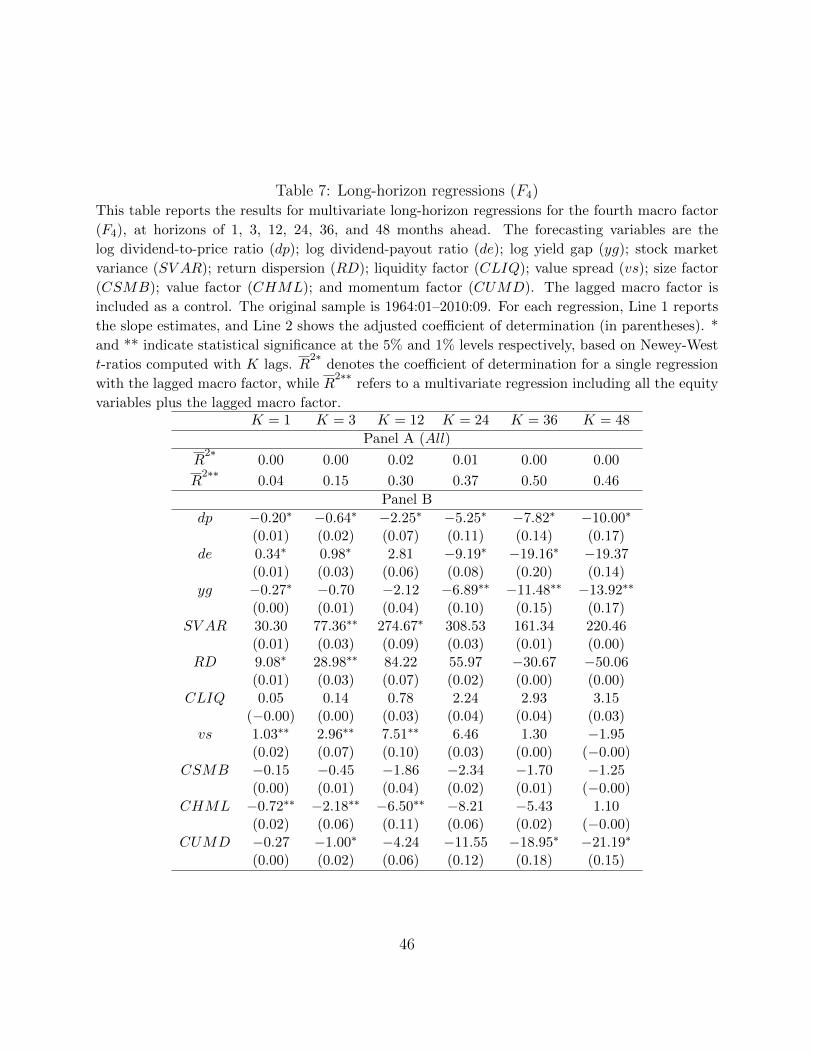
Our results from in-sample long-horizon regressions show that the contribution of the eq-

uity variables in predicting the macro factors tends to increase with the forecasting horizon,

and thus is especially relevant at long horizons, after accounting for the lagged macro fac-

tors. The yield gap, the value factor, and especially the dividend-payout ratio, are relevant

forecasters of future output. On the other hand, the most successful variable in forecast-

ing inflation is the dividend payout-ratio. Moreover, it turns out that the dividend yield,

dividend-payout ratio, yield gap, and the momentum factor have forecasting ability for the

2

housing factor at long horizons.

Third, we also conduct an out-of-sample forecasting analysis, in contrast with most of the

related literature, which relies on in-sample regression analysis. Contrary to the evidence

from the in-sample regressions, the out-of-sample forecasting power tends to be stronger

at short and intermediate forecasting horizons. Furthermore, by comparing with the in-

sample results, we observe that the predictive power at long horizons associated with the

yield gap, value factor, momentum factor, and especially the dividend payout ratio, does

not subsist out-of-sample. Moreover, several variables that do not forecast the factors in the

in-sample regressions have some out-of-sample forecasting power at long horizons—dividend

yield, stock market variance, return dispersion, and the liquidity factor. Taking into account

both the in-sample and out-of-sample performance, the stock-bond yield gap seems to be

the variable with the best overall performance.

Fourth, we put in perspective the evidence on the forecasting ability of the equity vari-

ables, by analysing the predictability of interest rate variables for the macro factors. The

comparison across both sets of variables yields mixed results: the term spread underper-

forms the dividend-payout ratio in forecasting output at long horizons, but it significantly

outperforms all equity predictors in terms of forecasting future inflation. However, the bond

predictors clearly lag behind most of the equity predictors when it comes to predicting future

housing activity.

Fifth, we evaluate the dynamic correlation between expectations of future equity cash

flows and the macro factors. The results suggest that there is in some cases a statistically

significant positive correlation between cash flow news and measures of future economic activ-

ity. However, these correlations are relatively small in magnitude, and thus not economically

significant.

3

The paper proceeds as follows. In Section 2, we present the macro factors and financial

variables used in the subsequent sections. Section 3 shows the in-sample predictability re-

sults, while Section 4 presents the out-of-sample predictability results. The predictability

from interest rate variables is analysed in Section 5. Section 6 analyses the dynamic correla-

tion between expectations of future equity cash flows and the macro factors. Finally, Section

7 concludes.

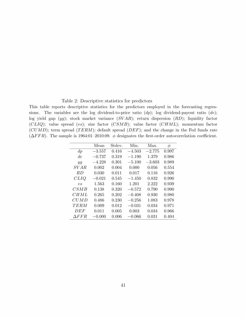
2 Data and variables

2.1 Macro factors

In the empirical analysis, we use the common macro factors estimated in Maio and Philip

(2013a) from a large set of 107 U.S. macroeconomic variables spanning the period from

1964:01 to 2010:09. This data set was originally used by Stock and Watson (2002, 2006),

and consists of seven broad categories, namely: output and income; employment and labor

force; housing ; manufacturing, inventories and sales ; money and credit ; exchange rates ;

and prices. By using asymptotic principal component analysis, Maio and Philip (2013a)

estimate four factors that summarize the common variation in the original macro variables.1

The descriptive statistics in Table 1 show that the four factors jointly explain around 36%

of the variation in the macroeconomic time-series, with the first factor explaining the bulk

of the common variation (18%).

The autocorrelations presented in Table 1 show that the first factor is relatively per-

sistent (autocorrelation coefficients around 0.71), while F3 presents a significantly smaller

1Other papers that use common macro factors, estimated by principal components analysis, to studythe interaction between the economy and the stock market include Ludvigson and Ng (2007) and Maio andPhilip (2013b).

4

autocorrelation (0.38). On the other hand, the fourth factor is not serially correlated, while

F2 contains a small negative autocorrelation (-0.20).

Panel B in Table 1 reports the highest coefficient of determination (R2) per category from

simple univariate regressions of the estimated factors against each of the 107 macroeconomic

variables,

Fjt = τi,jyit + ui,jt, j = 1, ..., 4, i = 1, ..., 107, (1)

where yit represents the ith original macro variable and ui,jt denotes an i.i.d. error term.

The results indicate that each of these four factors has to some extent an economic interpre-

tation in the sense that they are more correlated with a specific group of macro variables.

Specifically, the first common factor (F1) is an output factor since it is highly correlated

with the output and income, employment and labor force, and manufacturing, inventories,

and sales categories. The second factor (F2) is basically an inflation factor since it is highly

correlated with the prices category. On the other hand, the third factor (F3) may be classi-

fied as an output and housing factor, given that it is more correlated with the housing and

manufacturing, inventories, and sales categories. Finally, the fourth factor (F4) seems to

drive variation in the real estate sector since it is more correlated with the housing category.

2.2 Stock market variables

One of the key innovations in this study is to employ a wide range of stock market indicators

to forecast macro variables. The first group of equity variables contains indicators that

are used in the return predictability literature to forecast the stock market (excess) return.

The first variable is the aggregate log dividend-to-price ratio (dp, Fama and French (1988,

1989), Campbell and Shiller (1988)). dp is computed as the log ratio of the sum of annual

5

dividends to the level of the Standard and Poors (S&P) 500 index. The second variable is the

aggregate log dividend-payout ratio (de, Lamont (1998)), which represents the log ratio of

annual dividends to earnings of the S&P 500 index. The price, dividend, and earnings data

associated with the S&P 500 index are available from Robert Shiller’s website. A variable

related to dp is the log equity-bond yield spread, denoted as log yield gap (yg, Asness (2003),

Bekaert and Engstrom (2010), and Maio (2013d)). Following Maio (2013d), yg is computed

as yg = dp− 10y, where y is the log yield on a ten-year Treasury bond. The bond yield data

are available from St. Louis Fed. The fourth equity variable is the realized stock market

variance (SV AR, Guo (2006), Goyal and Welch (2008), Maio and Santa-Clara (2012)), which

is available from Amit Goyal’s website. A related variable is the stock return dispersion (RD,

Stivers and Sun (2010), Maio (2012)). RD represents a three-month moving average of the

cross-sectional standard deviation of the returns on 100 portfolios sorted on size and book-

to-market. The portfolio return data are from Kenneth French’s website. The next variable

is the value spread (vs, Campbell and Vuolteenaho (2004), Maio and Santa-Clara (2012)),

which represents the spread in the log book-to-market ratios of small-value and small-growth

portfolios. For details on the construction of vs, see the online appendix to Campbell and

Vuolteenaho (2004).

The remaining four variables are related to risk factors used in the empirical asset pricing

literature to explain the cross-section of stock returns. The first two factors are the size

(SMB) and value (HML) factors from Fama and French (1993, 1996). The third variable

is the return momentum factor (UMD) from Carhart (1997). The data on these three risk

factors are retrieved from Kenneth French’s webpage. Finally, we employ the non-traded

liquidity factor (LIQ) from Pastor and Stambaugh (2003). The data on LIQ are obtained

from Lubos Pastor’s Web site.

6

Following Maio and Santa-Clara (2012), we use a 60-month rolling sum of the original

factors. For example, in the case of SMB, the rolling cumulative return is given by

CSMBt =t∑

s=t−59

SMBs, (2)

and similarly for CHML, CUMD, and CLIQ. Since these return-based factors are highly

volatile, by using a rolling sum we are able to measure a more stable dynamic correlation

between these variables and the macro factors.

The descriptive statistics associated with the equity variables, presented in Table 2, show

that dp, de, and yg are very persistent, as indicated by the autocorrelation coefficients above

0.98. The cumulative returns (CSMB,CHML,CUMD) and the liquidity factor also exhibit

serial correlations very close to one. On the other hand, both RD and vs are less persistent

over time than the other variables, with autoregressive coefficients below 0.94. By far the

least persistent variable is SV AR, with an autocorrelation of 0.55.

Figure 1 displays the time-series of the equity risk factors, CSMB, CHML, CUMD,

and CLIQ. We can see that all the factors are quite volatile, especially the size and value

factors, which exhibit large up-and-down swings. After the significant drop in the second

half of the 1990s, both the rolling size and value premiums have rebounded before initiating

a significant decline in the mid 2000s. On the other hand, both the liquidity and especially

the momentum factor registered a significant decline around or at the end of the recent bear

equity market.

Table 3 presents the contemporaneous correlations between the stock market variables

and the four macro factors. The equity variables are not significantly correlated with the

macro factors, as most correlations are below 0.20 in magnitude. The first factor is weakly

7

negatively correlated with de, SV AR, RD, and vs, while the inflation factor shows corre-

lations very close to zero against all equity predictors. On the other hand, the third factor

is slightly positively correlated with both de and vs, whereas the housing factor (F4) has a

small positive correlation with SV AR.

3 In-sample predictability

In this section, we analyze the in-sample (IS) predictability of the different stock market

variables for each of the four common factors described in the previous section.

3.1 Methodology

We run multivariate long-horizon predictive regressions of the form,

Fj,t+1,t+K = aK + bKxt + cKFj,t + ut+1,t+K , j = 1, ...6, (3)

where Fj,t+1,t+K ≡ Fj,t+1 + ...+Fj,t+K is the cumulative sum of the j-th macro factor over K

months in the future, and xt is one of the equity variables known at time t used as predictor.

The forecasting horizons are 1, 3, 12, 24, 36, and 48 months ahead. We also estimate a

multivariate regression including all the predictors to gauge the joint forecasting power of

the equity variables.

It is important to note that in the regression above the current macro factor is one of the

predictors, as in Stock and Watson (2003), which allows one to assess if each of the equity

variables has predictive power for future macro variables in addition to the lagged macro

factor. The statistical inference for the slope estimates is based on the Newey and West (1987)

8

asymptotic t-statistics (computed with K lags), which correct for the heteroskedasticity and

serial correlation in the regression residuals (caused by the overlapping in the dependent

variable).

The t-stats associated with the slope, bK , represent a test of the statistical significance of

each predictor, while the adjusted coefficient of determination of the regression, R2, denotes

a measure of the joint economic significance of the equity variable and lagged macro factor in

forecasting the future realizations of the macro factor. To better assess the incremental fore-

casting power associated with the equity variable, we also estimate the adjusted coefficient

of determination from a univariate regression that excludes the equity variable:

Fj,t+1,t+K = aK + bKFj,t + ut+1,t+K , j = 1, ...6. (4)

3.2 Empirical results

The results for the forecasting regressions associated with the first factor (F1) are displayed

in Table 4. We can see that the current value of the factor has significant forecasting

ability for its future values at the nearest horizons (until 12 months), as indicated by the R2

estimates varying between 27% (K = 12) and 54% (K = 3). However, for horizons beyond

24 months this forecasting power disappears, as shown by the estimates of the coefficient of

determination very close to zero. The R2 values for the multivariate regressions including all

the predictors show a u-shaped pattern: the forecasting ability is quite large at short-horizons

(mostly driven by the lagged macro factor) with forecasting ratios above 50%, declining to

38% at intermediate horizons (K = 24), and increasing again at long horizons (K = 48) to

values above 50%. Therefore, the contribution of the equity variables is especially relevant

at intermediate and long horizons (K ≥ 24), as shown by the difference in the adjusted R2

9

against the single regression.

We proceed with the forecasting ability of each stock variable, which represents the core

of our empirical analysis. The log dividend yield does not help to forecast the output factor

as none of the slopes is significant at the 5% level. On the other hand, the log yield gap

clearly outperforms dp, forecasting an increase in future output at all horizons. For horizons

beyond three months, the coefficients associated with yg are significant at the 5% or 1%

levels. At long horizons (K ≥ 36), the forecasting ratios are around 16%, compared to R2

estimates around zero in the univariate regressions containing only the lagged macro factor.

Except the shortest horizons (K ≤ 3), the log dividend-payout ratio forecasts positive output

growth with the slopes being strongly significant (at the 1% level). The forecasting power

of d − e is even greater than that observed for yg, with R2 estimates above 30% at long

horizons (K ≥ 36).

Both SV AR and RD forecast a decline in future output, and this effect is statistically

significant at short and medium horizons (K ≤ 24), except the regression with SV AR

at K = 24. The values for the coefficient of determination are similar in the regressions

with either stock volatility measure and show only marginal predictive power relative to the

regressions including only the lagged macro factor. Yet, at long horizons (K ≥ 36) neither

SV AR nor RD helps to forecast the first macro factor, as indicated by the non-significant

slopes and the very low R2 estimates (below 5%), which lag behind the forecasting ability

from dp. None of the remaining equity predictors are significant predictors (at the 5% level)

of future output. The predictor showing the best performance at long horizons is CUMD,

with forecasting ratios around 8%, yet the respective slopes are not significant at the 5%

level.

The results for the second macro factor (inflation factor) are displayed in Table 5. The

10

lagged inflation factor has much less forecasting power for its future realizations than the

first macro factor as shown by the fact that the highest R2 estimate is now only 12% (at the

three-month horizon). Similarly to F1, the predictive ability of the lagged factor vanishes at

long horizons with R2 estimates below 5%. In the multivariate regression including all the

equity variables, the forecasting power tends to increase with the horizon, with forecasting

ratios varying between 4% (K = 1) and 45% (K = 36). Thus, as in the case of the output

factor, the value added of the joint equity variables for forecasting inflation is greater at

longer horizons (K ≥ 24).

Regarding the individual predictors, de forecasts a decline in future inflation, and the

slopes are statistically significant (at the 1% level) for horizons after 12 months. The coeffi-

cients of determination tend to increase with the forecasting horizon, varying between 4% at

K = 1 and 18% at K = 48, which compares to only 3% in the single forecasting regression.

Thus, the forecasting ability of the dividend-payout ratio for the second factor is economi-

cally significant at long horizons. yg is also negatively correlated with future inflation, but

the respective slope is only statistically significant at the 12-month horizon. Moreover, the

associated forecasting ratios are only marginally above the corresponding estimates in the

single regression containing only the lagged macro factor.

The value factor (CHML) forecasts a significant decline in future inflation for horizons

between 12 and 36 months. The highest fit is achieved at K = 24 (15%), which is similar

to the fit obtained in the regression with de. Still, at K = 36, CHML lags behind the

dividend-payout ratio with a R2 estimate of 8% (versus 17% in the bivariate regression

including de). The remaining equity variables do not help to forecast future inflation, as

indicated by the insignificant coefficients and quite low forecasting ratios. Among these

predictors, the variable with the highest forecasting power at long horizons is the liquidity

11

factor (R2 = 8%), yet the respective slopes are not significant at the 5% level.

The results for the third factor (output and housing factor) are displayed in Table 6.

The forecasting ability of the lagged output-housing factor for its future realizations declines

approximately with the forecasting horizon: the highest fit is achieved at K = 3 (24%) and

decreases to near zero R2 values for horizons beyond 12 months. On the other hand, the

joint forecasting power of the equity variables increases almost monotonically with horizon,

with forecasting ratios that vary between 18% (K = 1) and 50% (K = 36, 48). Thus, the

joint forecasting power of the equity predictors at long horizons is similar to the fit observed

for the regressions associated with the first macro factor. This similarity should be related

to the fact that both macro factors are related with output variables.

In terms of individual predictors, the dividend-payout ratio forecasts an increase in F3

at shorter horizons (K =≤ 12) and the respective slopes are statistically significant at

the one- and three-month horizons. The highest fit occurs at K = 3 with a R2 of 28%,

compared to 24% in the single regression containing the lagged macro factor. The yield gap

is negatively correlated with future output and housing activity at most horizons, yet only

at longer horizons (K ≥ 36) are the slopes statistically significant. At these horizons, the R2

estimates are around 10%, compared to zero values in the corresponding single regressions.

SV AR forecasts an increase in the housing-output factor, but only at K = 12 is the

slope statistically significant. The forecasting ratio is 18%, which represents an improvement

relative to the fit in the corresponding univariate regression (12%). In comparison, Return

dispersion outperforms SV AR at most horizons, and the respective slopes are significant at

horizons after three months. The largest contribution of RD occurs at K = 24, with an R2 of

12%, compared to 2% in the single regression, indicating that the cross-sectional variance of

stock returns helps to predict F3 at this horizon. The liquidity factor is positively correlated

12

with future housing and output at intermediate and long horizons, but only at K = 48 is the

coefficient significant at the 5% level. The corresponding forecasting ratio is 7%, compared

to zero in the single regression.

The positive slopes associated with vs are strongly significant at most horizons, except

the longest horizon. At intermediate horizons (K = 12, 24), the fit is similar to the one

obtained in the regression with RD. On the other hand, the value factor forecasts a decline

in F3 and the slopes are significant (5% or 1% level) at all forecasting horizons. At longer

horizons (K ≥ 24), CHML outperforms all the other predictors with R2 estimates around

or above 15%. This shows that the forecasting power associated with the value factor is

economically significant at the longer horizons. CUMD is also positively correlated with

future housing and output activity, although the slopes are statistically significant only at

the 12-month horizon. The corresponding R2 estimate is 16%, which is slightly above the fit

in the single regression with the lagged macro factor (12%).

In the case of the fourth factor (Table 7), the lagged housing factor basically has no

forecasting power over its future realizations as the R2 estimates in the single regressions

are all near zero. In contrast, the equity variables have strong joint predictive power for the

housing factor, especially at long horizons (K ≥ 36), with forecasting ratios around 50%.

Both dp and yg forecast a decrease in housing activity at all horizons, and the respective

slopes are statistically significant at most horizons (the exceptions are for yg at K = 3, 12).

Both variables offer a similar forecasting power, with the highest fit occurring at the longest

horizon (17% in both cases). On the other hand, de is positively correlated with the housing

factor at short horizons (K ≤ 12), but this correlation turns negative for horizons greater

than 12 months. The respective slopes are statistically significant, except at the 12-month

horizon. The largest amount of predictability from de is achieved at K = 36 with a fore-

13

casting ratio of 20%, slightly higher than the fit in the corresponding regressions with dp or

yg.

Both SV AR and RD (at most horizons) forecast an increase in the housing factor,

but only at short horizons (K ≤ 12) are the slopes statistically significant. The highest

forecasting power from both variables is achieved at K = 12 with R2 estimates of 9% and

7% for SV AR and RD respectively, above the fit of the corresponding univariate regression

(2%). The value spread is also positively correlated with the fourth factor and the slopes

statistically significant (1% level) for horizons until 12 months. Similarly to both SV AR

and RD, the highest amount of predictability occurs at K = 12, with a forecasting ratio of

10%.

The equity risk factors (CHML and CUMD) are negatively correlated with the housing

factor. However, in the case of CHML the slopes are not statistically significant at long

horizons (K ≥ 24), while in the case of CUMD the slopes are significant only at the three-

month and long horizons (K = 36, 48). CHML outperforms CUMD at the nearest horizons

while a converse relation holds for longer horizons, as indicated by the R2 estimates between

12% (K = 24) and 18% (K = 36) in the regressions with CUMD. Hence, the predictive

ability of the momentum factor is economically significant at long horizons.

The results from the in-sample long-horizon regressions can be summarized as follows.

At short horizons, the output factor is basically predicted by its past realizations, while

at long horizons, yg, and especially de, are relevant forecasters of future output. On the

other hand, the most successful variable in forecasting inflation is the dividend payout ratio,

especially at long horizons. The value risk factor outperforms all the other predictors in

terms of forecasting the housing-output factor, although the yield gap has also predictive

power at long horizons. Moreover, all dp, de, yg, and the momentum factor have forecasting

14

ability for the housing factor at long horizons. We also conclude that the contribution of

the equity variables in predicting the macro factors tends to increase with the forecasting

horizon, and thus is especially relevant at long horizons.

4 Out-of-sample predictability

In this section, we evaluate the out-of-sample (OS) predictive power of each equity variable

for the six macro factors. The OS regressions enable us to evaluate the parameter instability

over time in the IS regressions, and also to simulate real-time forecasting. Nevertheless, these

results should be interpreted with caution, given the low statistical power of OS regressions

when the forecasting horizon increases. The reason is that there are significantly fewer usable

observations at longer horizons, which is especially relevant in the first recursive regressions

conducted for the earlier periods (see Inoue and Kilian (2004)).

4.1 Methodology

To assess the OS predictability of the equity variables, the null (or restricted) model consid-

ered is the predictive regression containing only the lagged macro factor, while the alternative

(or unrestricted) model incorporates each equity variable:

H0 : Fj,t+1,t+K = aK + bKFj,t + uR,t+1,t+K , j = 1, ...6, (5)

Ha : Fj,t+1,t+K = aK + bKxt + cKFj,t + uU,t+1,t+K , j = 1, ...6.

15

The first OS measure is the OS coefficient of determination,

R2OS = 1 − MSEU

MSER

, (6)

where MSEU = 1TOS

∑TOS

t=1 u2U,t+1,t+K denotes the mean-squared forecasting error associated

with the unrestricted model, and MSER represents the same for the restricted model. TOS

is the number of observations in the evaluation (or out-of-sample) period. The OS R2 is

positive whenever MSEU < MSER; that is, the forecasting squared errors associated with

the augmented regression have lower magnitude than those associated with the restricted

regression.

The second OS evaluation measure is the F -test from McCracken (2007),

MSE-F = (TOS −K + 1)MSER −MSEU

MSEU

, (7)

where the null hypothesis is that the MSE associated with the restricted model is less than

or equal to that of the unrestricted model. The alternative hypothesis is that the MSE

associated with the unrestricted model is below the value from the restricted model.

The third OS test statistic is the encompassing test proposed by Harvey, Leybourne, and

Newbold (1998) and Clark and McCracken (2001),

ENC-NEW =TOS −K + 1

TOS

∑TOS

t=1

(u2R,t+1,t+K − uR,t+1,t+K uU,t+1,t+K

)MSEU

, (8)

in which the null hypothesis is that the restricted model encompasses the unrestricted model;

that is, the unrestricted model cannot improve the restricted model in forecasting future

macro factors. The alternative hypothesis is that the unrestricted model has additional

16

information that can improve the forecast obtained from the restricted model. The statistical

inference associated with the MSE-F and ENC-NEW statistics is based on the critical values

derived in McCracken (2007) and Clark and McCracken (2001), respectively.

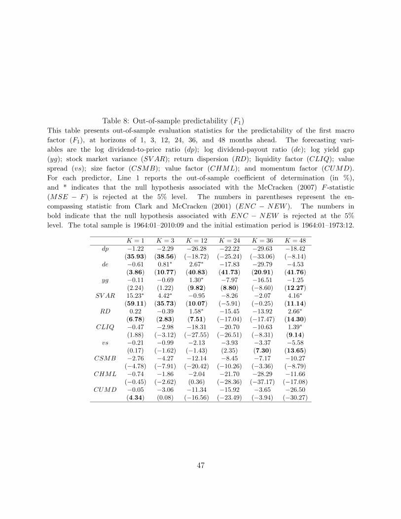
4.2 Empirical results

The results for the OS statistics associated with the first factor are in Table 8. At short

horizons, SV AR contains predictive power for the output factor as indicated by the positive

OS R2 estimates (15.23% and 4.42% at K = 1 and k = 3 respectively) and the rejection of

the null hypothesis associated with either MSE-F or ENC-NEW. The dividend payout ratio

also delivers a positive forecasting ratio at K = 3, yet it does not help to forecast F1 at the

one-month horizon. On the other hand, the forecasting ratio in the regression with RD is

marginally positive (0.22%), but the the model fails to pass the MSE-F test. At K = 12, it

turns out that de, yg, and RD have predictive ability for the output factor, with R2 estimates

above 1%. The largest degree of predictability comes from de, with a forecasting ratio of

2.67%. At the 48-month horizon, both volatility variables and the liquidity factor help to

forecast the output factor, with R2 estimates of 4.16%, 2.66%, and 1.39% for SV AR, RD,

and CLIQ respectively. Moreover, the null associated with either test is rejected at the 5%

level in the regressions with these three predictors.

The results in Table 9 show that the OS forecasting ability of all the equity predictors

for the second factor (inflation) is quite weak, as most OS R2 estimates are negative. The

few exceptions are SV AR at K = 12 (1.01%), and RD (0.28%) and CHML (3.90%), both

at K = 48. Nevertheless, in all three cases the null-hypothesis associated with MSE-F is

not rejected at the 5% level, while the model fails to pass the ENC-NEW test in the case of

RD.

17

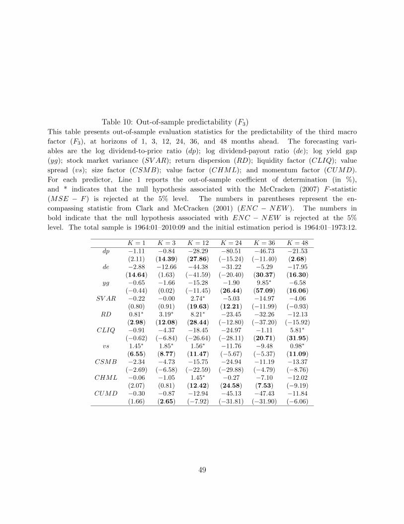
The results for the third factor are displayed in Table 10. At short and intermediate

horizons (K ≤ 12), both RD and vs have OS predictive ability for the third factor, as

indicated by the positive forecasting ratios and the non-rejection of the null hypotheses

associated with both MSE-F and ENC-NEW. At K = 1, vs outperforms RD, while a

converse relation holds at the three- and 12-month horizons. Both SV AR and CHML also

produce positive R2 estimates and pass both tests at K = 12, although for shorter horizons

the forecasting ratios associated with these two predictors are negative. At long horizons

(K ≥ 36), it turns out that yg (K = 36) and both CLIQ and vs (both at K = 48) are the

only predictors with positive forecasting ability for the housing-output factor. The greatest

forecasting power is achieved in the regressions with yg (K = 36) and RD (K = 12) with

R2 estimates of 9.85% and 8.21% respectively.

Regarding the fourth factor (Table 11), at short horizons (K = 1, 3), both vs and CHML

have forecasting ability for future housing activity, as indicated by the positive values for the

coefficient of determination (above 1%) and the rejection of the null hypothesis associated

with either MSE-F or ENC-NEW. Moreover, de (at the three-month horizon) and SV AR

(at the one-month horizon) help to forecast the housing factor, although the forecasting

ratios are below 1% in both cases. The regression with RD also produces marginal positive

coefficients of determination, yet the model does not pass either the ENC-NEW (K = 1) or

the MSE-F (K = 3) tests. At the 24-month horizon, both yg and CUMD help to forecast

F4, as shown by the R2 estimates of 3.09% and 2.74% respectively, and the fact that the

corresponding predictive regressions pass both statistical tests. At K = 12, SV AR produces

a marginal positive forecasting ratio, yet the null associated with ENC-NEW is not rejected

at the 5% level.

At K = 36, only one predictor (yg) has predictive ability, with a forecasting ratio of

18

1.63%. SV AR also delivers a positive coefficient of determination (0.75%), yet the model

does not pass the encompassing test. On the other hand, at K = 48, we observe the largest

degree of OS predictability, with five predictors (dp, yg, SV AR, RD, and CSMB) helping

to forecast housing activity. yg produces the highest fit with a forecasting ratio of 9.04%,

followed by dp (5.53%). In the regression with vs, we have a marginally positive R2 (0.27%),

yet the null associated with MSE-F is not rejected at the 5% level.

The results in this section show that, contrary to the evidence from the IS regressions,

the OS forecasting power tends to be stronger at short and intermediate forecasting horizons.

Furthermore, consistent with previous evidence (e.g., Maio (2013b, 2013d)) the OS evidence

for all four factors shows that it is easier to pass the ENC-NEW test than the MSE-F test

for most equity predictors. Overall, by comparing the results in this section with the IS

results from the previous section, we observe that the predictive power at long horizons of

yg (for F1), CHML (for F3), CUMD (for F4), and especially de (for F1, F2, and F4) does

not subsist out-of-sample.

Moreover, several variables that do not forecast the factors in the IS regressions at long

horizons have OS forecasting power for some of the macro factors (F1 and F4), like SV AR,

RD, CSMB, and the liquidity factor. These results are partially consistent with previous

evidence in the related literature. Specifically, Loungani, Rush, and Tave (1990) find that re-

turn dispersion forecasts an increase in unemployment. Næs, Skjeltorp, and Ødegaard (2011)

show that a decrease in stock market liquidity leads to lower future output growth, condi-

tional on several controls (term spread, credit spread, market volatility, and excess market

return).2 Moreover, several studies (e.g., Campbell, Lettau, Malkiel, and Xu (2001), Bloom

2In related work, Beber, Brandt, and Kavajecz (2011) show that sector orderflow can predict the state ofthe economy. Specifically, large orderflow into the material sector forecasts an expanding economy, while largeorderflow into consumer discretionary, financials, and telecommunications forecasts a contracting economy.

19

(2009), Bakshi, Panayotov, and Skoulakis (2011), and Fornari and Mele (2011)) indicate

that alternative measures of stock market volatility help to forecast the economy.3 Vassalou

(2003) provides evidence that size/book-to-market portfolios (used in the construction of

SMB and HML) provide information for future GDP growth, while Liew and Vassalou

(2000) provides similar evidence for both SMB and HML.

5 Credit markets and the economy

In this section, we use alternative predictors that are related to short-term interest rates and

bond yields in order to forecast the macro factors. Using variables from the credit markets

allows us to put in perspective the evidence on the forecasting ability of the equity variables

analysed in the previous section. Moreover, most of the related literature has focused on

bond market predictors to forecast the economy, rather than stock market indicators (see

the survey in Stock and Watson (2003)).

The new predictors are the first-difference in the Fed funds rate (∆FFR); the term spread

or slope of the yield curve (TERM); and the default spread (DEF ). Among these, both

TERM and DEF have been widely used to forecast future economic activity or inflation

(see, for example, Harvey (1988, 1989), Stock and Watson (1989), Mishkin (1990), Estrella

and Hardouvelis (1991), Jorion and Mishkin (1991), Estrella and Mishkin (1998), and Estrella

(2004) on the term spread, and Bernanke (1983), Stock and Watson (1989), Gertler and Lown

(1999), and Gilchrist, Yankov, and Zakrajsek (2009) on the default spread). Less attention

has been devoted to using short-term interest rates to forecast future output, with Bernanke

and Blinder (1992) and Ang, Piazzesi, and Wei (2006) representing two exceptions. TERM

3In related work, Allen, Bali, and Tang (2012) show that a measure of aggregate systemic risk, related tovalue-at-risk, conveys information about the future state of the economy.

20

is computed as the yield spread between the ten-year and the one-year Treasury bonds, and

DEF denotes the yield spread between BAA and AAA corporate bonds from Moody’s. The

interest rate and bond yield data are available from St. Louis Fed Web page.

5.1 In-sample predictability

The in-sample predictability results associated with the first two factors are displayed in

Table 12. In the case of the first factor, the R2 estimates of the multivariate regressions in-

cluding the three interest rate predictors (plus the lagged macro factor) have an approximate

declining monotonic pattern with the forecasting horizon, varying between 57% (K = 3) and

12% (K = 48). The largest contribution of the three interest rate predictors for forecasting

F1 occurs at the 24- and 36-month horizons, with R2 estimates (in the multivariate regres-

sions) of 25% and 22% respectively, compared to only 8% and 1% in the corresponding single

regression containing the macro factor.

The term spread forecasts an increase in the output factor and the slopes are strongly

significant at most horizons, with the sole exception of the one-month horizon, in which the

coefficient is not significant at the 5% level. The largest contribution in terms of forecasting

power of TERM is achieved at K = 24 and K = 36, with forecasting ratios of 24% and 21%

respectively, which are only marginally below the adjusted coefficients of determination in

the corresponding multiple regressions including all three interest rate predictors. The neg-

ative coefficient associated with DEF at the one-month horizon is statistically significant.

However, the R2 values from the bivariate regression are very similar to the corresponding

estimates from the univariate regressions, indicating that the credit spread does not add rele-

vant forecasting power to the lagged factor. At horizons beyond three months the coefficients

associated with DEF turn positive, but the slopes are not significant at the 5% level. On

21

the other hand, the change in the Fed funds rate predicts a significant decline in the output

factor for horizons beyond three months, yet the forecasting ratios are significantly lower

than in the bivariate regressions with TERM , especially at the 24- and 36-month horizons.

Moreover, these estimates are only marginally higher than the corresponding values in the

single regression, thereby indicating that such predictability is not economically significant.

Thus, the term spread remains the only economically significant forecaster of future output

at intermediate and long horizons.

Regarding the second factor, the joint bond predictors add forecasting power for future

inflation at horizons beyond 12 months: the forecasting ratios vary between 12% (K = 48)

and 25% (K = 24), which compare with 0% and 8% in the corresponding single regressions

including only the lagged macro factor. The term spread forecasts a decline in future inflation

for horizons beyond one month and the slopes are significant (5% or 1% levels) for K ≥

12. The R2 estimates in the bivariate regression tend to increase with horizon, reaching

a maximum of 26% (compared to 2% in the univariate regression) at K = 36. Thus, the

forecasting power of TERM for future inflation has large economic significance at long

horizons. On the other hand, the slopes associated with DEF alternate in sign, but are not

statistically significant at any horizon. ∆FFR forecasts a significant increase in inflation at

the 48-month horizon, yet the R2 is relatively modest (4%). Therefore, as for the output

factor, the term spread is the only economically significant predictor of future inflation at

intermediate and long horizons.

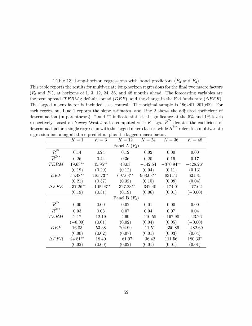
Table 13 shows the predictability results for the third and fourth factors. In the case of

the third factor, the multivariate regressions including all the interest rate variables show

a near monotonic decline in fit, with R2 estimates varying between 44% (K = 3) and 17%

(K = 48). However, the joint forecasting ability of the interest rate predictors is economically

22

significant at all horizons, as shown by the sizable differences between the forecasting ratios in

the multiple and corresponding single regressions containing only the lagged macro factor.

This contrasts with the first two factors, for which the joint bond variables do not add

relevant forecasting power at short horizons.

For horizons until 12 months, it happens that TERM predicts an increase in future

housing-output activity, and the respective coefficients are significant for K ≤ 3. At short

horizons (K = 1, 3), the R2 estimates are slightly above the fit in the corresponding single

regressions. However, after 12 months, the slopes associated with TERM turn negative

and there is statistical significance at long horizons (K ≥ 36). At these horizons, the

coefficient of determination is above 10%, compared to zero estimates in the corresponding

single regressions. Thus, the economic significance of the predictability associated with

TERM is greater at long horizons.

The default spread forecasts an increase in the housing-output factor, with the slopes be-

ing significant except at long horizons (K ≥ 36). The largest forecasting power is achieved at

the three- and 12-month horizons, with R2 above 30%, well above the fit in the correspond-

ing single regressions. Thus, the predictability associated with the default spread for the

third factor is economically significant, especially at short and intermediate horizons. The

change in the Fed funds rate is negatively correlated with future housing-output activity at

all horizons, although this effect is only statistically significant at horizons upto 12 months.

The largest fit occurs at the three-month horizon with an R2 of 31%, which is marginally

above the fit in the regression with TERM , but below the estimate associated with DEF .

At long horizons, there is no predictive ability as the R2 estimates are around zero and the

slopes are not significant.

Regarding the fourth factor, the bond predictors do not add much forecasting power as

23

a whole, since the R2 estimates are quite modest at all forecasting horizons. The highest

fit is achieved at K = 12 and K = 36, with a forecasting ratio of 7% in both cases, which

compares to 2% and 0% in the corresponding single regressions. Thus, in contrast to the first

three factors the joint predictability from the bond variables is not economically significant.

Specifically, the slopes associated with both TERM and DEF alternate in sign between

short and long horizons, but there is no statistical significance at any horizon. Thus, neither

spread conveys information about future real estate activity. On the other hand, ∆FFR

forecasts an increase in F4 at both short (K = 1, 3) and long (K = 36, 48) horizons, and

the respective slopes are significant at both the one- and 48-month horizons. However, the

forecasting ratios are quite small (around 1-2%), showing that this predictive relation is not

economically significant.

In sum, the in-sample results show that the largest contribution of the bond predictors

in forecasting the macro factors occurs at intermediate and long horizons, similarly to the

evidence for the equity predictors in Section 3. In terms of individual predictive perfor-

mance, the term spread helps to forecast both the output and inflation factors at middle

and long horizons. On the other hand, all three interest rate variables help to forecast the

housing-output factor, although the default spread tends to outperform the other predictors,

especially at short and intermediate horizons. Finally, none of the predictors significantly

helps to forecast the housing factor.

By comparing with the in-sample results for the equity variables, discussed in Section

3, the results tend to be mixed. Regarding the first factor, it follows that the term spread

underperforms relative to the dividend-payout ratio at long horizons (K ≥ 36). However,

TERM compares favorably with the other equity predictors, including yg, in forecasting

future output. Moreover, the term spread outperforms all equity predictors for forecasting

24

future inflation at most horizons. In what concerns the third factor, it turns out that both

DEF and ∆FFR outperform the best performing equity predictors (CHML and yg) at

short and intermediate horizons (K ≤ 12). However, at long horizons (K ≥ 36) a converse

relation holds up. Finally, the bond predictors clearly lag behind most of the equity predictors

in terms of predicting future housing activity.

5.2 Out-of-sample predictability

We also analyse the OS forecasting ability of the bond predictors for the four macro factors.

The OS statistics associated with the first two factors are shown in Table 14. The results

show that TERM has forecasting ability for the first factor at horizons upto 12 months: the

forecasting ratios vary between 5.05% (K = 1) and 10.87% (K = 3), and in all three cases

the forecasting model passes both the MSE-F and ENC-NEW tests. On the other hand,

the default spread cannot predict the output factor out-of-sample as all the R2OS estimates

are negative. In the regressions containing the innovation in the Fed funds rate, we obtain

positive forecasting ratios at the one- and 12-month horizons, yet only at K = 12 are both

null hypotheses rejected at the 5% level. The OS forecasting power for the inflation factor is

quite poor since only in one case do we obtain a positive forecasting ratio: in the regression

with TERM at K = 12, the R2OS estimate is 5.45% and the model passes both the MSE-F

and ENC-NEW tests at the 5% level.

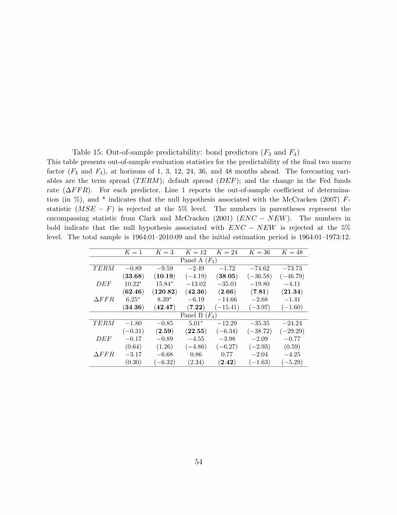
Regarding the third factor, the results in Table 15 show that both ∆FFR, and especially

DEF , have strong OS predictive power at short horizons (K = 1, 3). The R2OS estimates

are positive in all four cases, varying between 6.25% (∆FFR, K = 1) and 15.84% (DEF ,

K = 3). Moreover, in the regressions with either of these two predictors the null associated

with either MSE-F or ENC-NEW is rejected. Similarly to the inflation factor, the OS

25

forecasting ability for the housing factor is rather weak. Only in one case (TERM , K = 12)

do we obtain both a positive forecasting ratio (5.01%) and the rejection of the null in both

statistical tests. In the regressions with the change in the Fed funds rate at the 12- and

24-month horizons we also observe slightly positive R2OS estimates, yet the model does not

pass the MSE-F test.

By comparing with the IS results discussed above, we observe that the IS predictive power

of the bond predictors at long horizons does not subsist out-of-sample. This is especially

relevant for the term spread in forecasting the first three factors. Thus, only at short horizons

(K ≤ 12) are the interest rate variables valid OS predictors for the macro factors. At short

horizons, the main difference from the IS regressions is that TERM has no OS forecasting

power for the third factor, although it helps to predict the housing factor at the 12-month

horizon.

In terms of comparing with the OS predictive performance of the equity variables, the

results are again mixed. Regarding the first factor, the term spread tends to offer better

OS predictability than the equity indicators at near horizons (K ≤ 12). The sole exception

is against SV AR at the one-month horizon, which produces a R2OS estimate of 15.23%

(versus 5.05% for TERM). Nevertheless, at the 48-month horizon, there are several equity

predictors with positive OS forecasting power (SV AR, RD, and CLIQ), unlike any of the

bond predictors. In what concerns the inflation factor, it turns out that the term spread helps

to forecast inflation at the 12-month horizon. This is in contrast to the equity predictors,

which mostly produce negative forecasting ratios.

At short horizons (K ≤ 3), both the default spread and the change in the Fed funds rate

do better than the best performing equity predictors (RD and vs) in predicting the third

factor. However, at long horizons (K ≥ 36), there are several equity variables that help

26

to forecast the housing-output factor, in contrast to the interest rate predictors. Regarding

the fourth factor, as in the comparison of the IS results, the bond predictors clearly lag

behind the equity predictors. The only exception is the model with TERM at the 12-month

horizon.

6 Macro variables and expectations about future cash-

flows

In this section, we evaluate the dynamic correlation between expectations of future equity

cash flows and the macro factors. To the extent that equity earnings, and thus dividends,

are positively correlated to economic activity, we expect current expectations of future cash

flows (dividends) to forecast the macro factors, at least those more directly related with

real economic activity, like the output and housing factors. In related work, Maio and Philip

(2013b) analyse whether the macro factors have an impact in the estimates of future expected

aggregate cash flows. The analysis pursued in this section goes in the other direction: it

analyses whether expected cash flows forecast future economic activity.

6.1 Methodology

To estimate future expected cash flows, we use the present-value relation derived in Campbell

(1991). In this framework, the innovation in the current excess log stock market return, ret+1,

can be decomposed into revisions of future expected excess log returns (discount-rate news)

27

and revisions in expectations of future log dividend growth (cash-flow news),

ret+1 − Et(ret+1) ≈ (Et+1 −Et)

∞∑j=0

ρj∆dt+1+j − (Et+1−Et)∞∑j=1

ρjret+1+j

≡ NCF,t+1 −NDR,t+1, (9)

where Et denotes the conditional expectation at time t; NCF,t+1 represents cash-flow news;

and NDR,t+1 denotes discount-rate news. Equation (9) represents a dynamic present-value

relation obtained from the definition of the stock market return and by imposing a terminal

no-bubble condition. This equation also assumes that the revision in future short-term

interest rates (interest rate news) represents a small component of the current unexpected

excess stock return, in line with the evidence from Campbell and Ammer (1993), Bernanke

and Kuttner (2005), and Maio (2013a). The parameter ρ is a discount coefficient linked to

the average aggregate log dividend-to-price ratio. Following previous work (Campbell and

Vuolteenaho (2004) and Maio (2013a, 2013c)), we fix ρ at 0.95112 , which corresponds to an

annualized dividend yield of approximately 5%.

As in Campbell (1991) and Campbell and Ammer (1993), we employ a first-order VAR

to identify both NCF and NDR. The state vector xt, which includes the excess log market

return and other variables that help to forecast ret+1, follows the following process,

xt+1 = Axt + εt+1, (10)

where A is the VAR coefficient matrix, and εt+1 is a vector of zero-mean shocks.4

4The VAR variables xt are previously demeaned, thus the vector of intercepts is not included in the VARspecification.

28

The components of the excess market return are then estimated as follows,

NDR,t+1 = e1′ρA (I − ρA)−1 εt+1 = ϕ′εt+1, (11)

NCF,t+1 = ret+1 − Et

(ret+1

)+NDR,t+1

=[e1′ + e1′ρA (I − ρA)−1

]εt+1 = (e1 +ϕ)′ εt+1, (12)

where e1 is an indicator vector that takes a value of one in the cell corresponding to

the position of the excess market return in the VAR; I is an identity matrix; and ϕ′ ≡

e1′ρA (I − ρA)−1 is the function that translates the VAR shocks into discount-rate news.

This represents the standard identification method conducted in the related literature, in

which cash-flow news is the residual component of the unexpected stock market return. Thus

we do not have to define a direct model for the dynamics of aggregate dividends.

To check the robustness of our results against the way cash-flow news is measured, we

conduct an alternative identification procedure in which cash-flow news is estimated directly,

and discount-rate news represents the residual component of the (unexpected) excess market

return (see Maio (2013a) and Maio and Philip (2013b)),

NCF,t+1 = e2′ (I − ρA)−1 εt+1 = λ′εt+1 (13)

NDR,t+1 = NCF,t+1 − [ret+1 − Et(ret+1)]

=[e2′ (I − ρA)−1 − e1′

]εt+1 = (λ− e1)′ εt+1, (14)

where e2 is an indicator vector that takes a value of one in the cell corresponding to the

position of log dividend growth in the VAR, and λ′ ≡ e2′ (I − ρA)−1 is the function that

translates the VAR residuals into cash-flow news.

29

The VAR state vector taken to the data is given by

xt ≡ [∆FFRt, TERMt, DEFt, ygt,det, SV ARt, RDt, vst,∆dt, ret ]′ . (15)

We use the same VAR specification under the two alternative identification methods to

enable the comparison between both methods. The inclusion of the log aggregate dividend

growth, ∆dt, is needed in order to identify cash-flow news under the alternative identification

procedure. The excess log stock return corresponds to the log return on the value-weighted

stock index, available from CRSP, in excess of the log one-month T-bill rate. The data on

the T-bill rate are from Kenneth French’s web page. The remaining state variables contain

some of the equity variables analysed in the previous sections, which are frequently used as

predictors of the excess market return (yg, de, SV AR, RD, and V S).5 We use yg instead

of dp since the former has greater forecasting power for the aggregate equity premium (see

Maio (2013d)). In addition to the equity variables, we use the three interest rate predictors

used in the previous section (∆FFR, TERM , and DEF ), which are frequently employed

in the return predictability literature to forecast the equity premium.6

In the first identification method, the variance decomposition (in percentage) for the

excess stock market return is given by

1 =Var (NCF,t+1)

Var[ret+1 − Et(ret+1)

] +Var (NDR,t+1)

Var[ret+1 − Et(ret+1)

] − 2 Cov (NCF,t+1, NDR,t+1)

Var[ret+1 − Et(ret+1)

]= 0.81 + 0.78 − 0.59. (16)

5See, for example, Maio (2013d) for the yield gap; Lamont (1998) for the dividend-payout ratio; Guo(2006) for the stock market variance; Maio (2012) for the stock return dispersion; and Campbell andVuolteenaho (2004) for the value spread.

6See, for example, Patelis (1997) and Maio (2013b) for the predictability associated with ∆FFR; Camp-bell (1987) and Fama and French (1989) for TERM ; and Keim and Stambaugh (1986) and Fama and French(1989) for DEF .

30

These results indicate that cash flow and discount rate news have a similar share in explaining

the variation in the excess market return.

The variance decomposition associated with the second identification method is given by

1 =Var (NCF,t+1)

Var[ret+1 − Et(ret+1)

] +Var (NDR,t+1)

Var[ret+1 − Et(ret+1)

] − 2 Cov (NCF,t+1, NDR,t+1)

Var[ret+1 − Et(ret+1)

]= 0.28 + 1.22 − 0.49. (17)

Thus, we obtain a significantly larger share for discount rate news than for cash flow

news in driving the excess stock market return, which should be a consequence of the low

forecasting power of our VAR for future aggregate dividend growth. These results provide

evidence that the identification method has an influence in the resulting estimates of both

NCF and NDR.

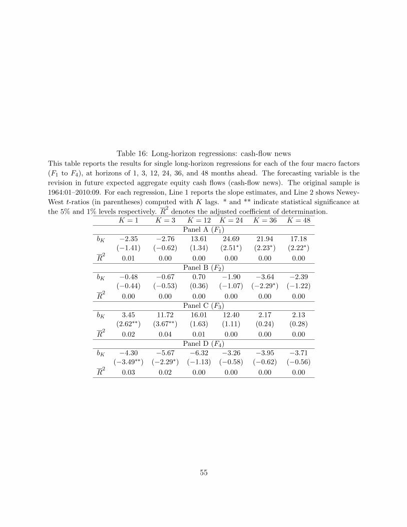
To assess the forecasting power of cash flow news for the macro factors, we conduct the

following single long-horizon regressions:

Fj,t+1,t+K = aK + bKNCF,t + ut+1,t+K , j = 1, ...6. (18)

6.2 Empirical results

The results for the forecasting regressions based on the benchmark identification of cash

flow news are presented in Table 16. Cash flow news is negatively correlated with the output

factor at short horizons horizon (K = 1, 3), but the slopes are not significant at the 5% level.

However, for horizons beyond 12 months, the coefficients become positive and statistically

significant. NCF also forecasts an increase in the output-housing factor, yet the slopes are

only significant at short horizons (K = 1, 3). Interestingly, the coefficients associated with

31

the inflation factor are negative at most horizons, although only at the 36-month horizon is

there statistical significance. On the other hand, cash flow news forecasts a decline in the

housing factor, but this effect is only statistically significant at the one- and three-month

horizons. The fit of the forecasting regressions for all the factors is quite low, as shown

by the R2 estimates: the highest forecasting power occurs for the third (K = 3) and fourth

(K = 1) factors, with forecasting ratios of 4% and 3% respectively. However, at long horizons

(K ≥ 24) the R2 estimates are all around zero.

The results based on the alternative identification of cash flow news are presented in

Table 17. NCF forecasts an increase in F1 at all horizons, and the slopes are significant at

short horizons, in contrast to the results based on the benchmark identification, for which

the predictability is concentrated at long horizons. In the regressions with either F2 or F3,

the slopes are negative in most cases except at short horizons. However, the slopes are not

significant at the 5% level. As in the benchmark identification, NCF is negatively correlated

with the future housing factor, but this effect is no longer significant. Similarly to the

benchmark case, the economic significance of the predictability associated with cash flow

news is quite low, as indicated by the R2 estimates close to zero. The largest fit occurs for

the first factor at short horizons, with forecasting ratios around 2-3%.

Overall, the results from this section suggest that there is a positive correlation between

cash flow news and output. However, these correlations are relatively small, as indicated by

the very low R2 estimates.

32

7 Conclusion

This paper attempts to conduct a comprehensive analysis of the forecasting role of stock

market indicators for macroeconomic variables. We contribute to this literature in several

ways. First, we use information from a large set of macroeconomic variables. In particular,

we use four common macro factors, estimated by applying principal component analysis

to a data set of 107 U.S. macroeconomic variables spanning the period from 1964:01 to

2010:09. The estimated macro factors are mainly related to aggregate output, inflation, and

the housing sector.

Our second innovation relative to the existent literature is that we use a more compre-

hensive set of equity indicators than most related papers. Specifically, we employ several

equity variables that are typically used in the stock return predictability literature: the log

dividend-to-price ratio, log dividend-payout ratio, stock-bond yield gap, stock market vari-

ance, stock return dispersion, and the value spread. In addition, we use equity risk factors

commonly employed in the cross-sectional asset pricing literature—the size, value, and mo-

mentum factors from Fama and French (1993) and Carhart (1997), and the liquidity factor

used in Pastor and Stambaugh (2003).

Our results from in-sample long-horizon regressions show that the contribution of the

equity variables in predicting the macro factors tends to increase with the forecasting horizon,

and thus is especially relevant at long horizons. The yield gap, the value factor, and especially

the dividend-payout ratio are relevant forecasters of future output. On the other hand, the

most successful variable in forecasting inflation is the dividend payout-ratio. Moreover, it

turns out that the dividend yield, dividend-payout ratio, yield gap, and the momentum

factor have forecasting ability for the housing factor at long horizons.

Third, we also conduct an out-of-sample forecasting analysis. Contrary to the evidence

33

from the in-sample regressions, the out-of-sample forecasting power tends to be stronger at

short and intermediate forecasting horizons. Furthermore, by comparing with the in-sample

results, we observe that the predictive power at long horizons associated with the yield gap,

value factor, momentum factor, and especially the dividend payout ratio does not subsist

out-of-sample.

Fourth, we put in perspective the evidence on the forecasting ability of the equity vari-

ables, by analysing the predictability of interest rate variables for the macro factors. The

comparison across both sets of variables yields mixed results: the term spread underper-

forms the dividend-payout ratio in forecasting output at long horizons, but it significantly

outperforms all equity predictors in terms of forecasting future inflation. However, the bond

predictors clearly lag behind most of the equity predictors when it comes to predicting future

housing activity.

Fifth, we evaluate the dynamic correlation between expectations of future equity cash

flows and the macro factors. The results suggest that there is in some cases a statistically

significant positive correlation between cash flow news and measures of future economic activ-

ity. However, these correlations are relatively small in magnitude, and thus not economically

significant.

34

References

Allen, L., T. Bali, and Y. Tang, 2012, Does systemic risk in the financial sector predict futureeconomic downturns? Review of Financial Studies 25, 3000–3036.

Andreou, E., E. Ghysels, and A. Kourtellos, 2012, Should macroeconomic forecasters usedaily financial data and how? Journal of Business and Economic Statistics, forthcoming.

Ang, A., M. Piazzesi, and M. Wei, 2006, What does the yield curve tell us about GDPgrowth? Journal of Econometrics 131, 359–403.

Asness, C., 2003, Fight the FED model: the relationship between future returns and stockand bond market yields, Journal of Portfolio Management 30, 11–24.

Bakshi, G., G. Panayotov, and G. Skoulakis, 2011, Improving the predictability of realeconomic activity and asset returns with forward variances inferred from option portfolios,Journal of Financial Economics 100, 475–495.

Barro, R., 1990, The stock market and investment, Review of Financial Studies 3, 115–131.

Beber, A., M. Brandt, and K. Kavajecz, 2011, What does equity sector orderflow tell usabout the economy? Review of Financial Studies 24, 3688–3730.

Bekaert, G., and E. Engstrom, 2010, Inflation and the stock market: Understanding the”Fed Model”, Journal of Monetary Economics 57, 278–294.

Bernanke, B., 1983, Nonmonetary effects of the financial crisis in the propagation of thegreat depression, American Economic Review 73, 257–276.

Bernanke, B., and A. Blinder, 1992, The Federal funds rate and the channels of monetarytransmission, American Economic Review 82, 901–921.

Bernanke, B., and K. Kuttner, 2005, What explains the stock market’s reaction to FederalReserve policy? Journal of Finance 60, 1221–1257.

Bloom, N., 2009, The impact of uncertainty shocks, Econometrica 77, 623–685.

Campbell, J., 1987, Stock returns and the term structure, Journal of Financial Economics18, 373–99.

Campbell, J., 1991, A variance decomposition for stock returns, Economic Journal 101,157–179.

Campbell, J., 1999, Asset prices, consumption and the business cycle, Handbook of Macroe-conomics, e.d. by John Taylor and Michael Woodford, Elsevier.

Campbell, J., M. Lettau, B. Malkiel, and Y. Xu, 2001, Have individual stocks become morevolatile? An empirical exploration of idiosyncratic risk, Journal of Finance 56, 1–43.

Campbell, J., and J. Ammer, 1993, What moves the stock and bond markets? A variancedecomposition for long-term asset returns, Journal of Finance 48, 3–26.

35

Campbell, J., and R. Shiller, 1988, The dividend price ratio and expectations of futuredividends and discount factors, Review of Financial Studies 1, 195–228.

Campbell, J., and T. Vuolteenaho, 2004, Bad beta, good beta, American Economic Review94, 1249–1275.

Carhart, M., 1997, On persistence in mutual fund performance, Journal of Finance 52, 57–82.

Chen, L., and L. Zhang, 2011, Do time-varying risk premiums explain labor market perfor-mance? Journal of Financial Economics 99, 385–399.

Clark, T., and M. McCracken, 2001, Tests of equal forecast accuracy and encompassing fornested models, Journal of Econometrics 105, 85–110.

Estrella, A., 2004, Why does the yield curve predict output and inflation? Economic Journal115, 722-744.

Estrella, A., and G. Hardouvelis, 1991, The term structure as a predictor of real economicactivity, Journal of Finance 46, 555–576.

Estrella, A., and F. Mishkin, 1998, Predicting U.S. recessions: Financial variables as leadingindicators, Review of Economics and Statistics 80, 45–61.

Fama, E., 1981, Stock returns, real activity, inflation, and money, American Economic Re-view 71, 545–565.

Fama, E., 1990, Stock returns, expected returns, and real activity, Journal of Finance 45,1089–1108.

Fama, E., and K. French, 1988, Dividend yields and expected stock returns, Journal ofFinancial Economics 22, 3–25.

Fama, E., and K. French, 1989, Business conditions and expected returns on stock andbonds, Journal of Financial Economics 25, 23–49.

Fama, E., and K. French, 1993, Common risk factors in the returns on stocks and bonds,Journal of Financial Economics 33, 3–56.

Fama, E., and K. French, 1996, Multifactor explanations of asset pricing anomalies, Journalof Finance 51, 55–84.

Fornari, F., and A. Mele, 2011, Financial volatility and economic activity, Working paper,University of Lugano.

Gertler, M., and C. Lown, 1999, The information content of the high yield bond spread forthe business cycle, Oxford Review of Economic Policy 15, 132–150.

Geske, R., and R. Roll, 1983, The fiscal and monetary linkage between stock returns andinflation, Journal of Finance 38, 1–33.

36

Gilchrist, S., V. Yankov, and E. Zakrajsek, 2009, Credit market shocks and economic fluctua-tions: Evidence from corporate bond and stock markets, Journal of Monetary Economics56, 471–493.

Goyal, A., and I. Welch, 2008, A comprehensive look at the empirical performance of equitypremium prediction, Review of Financial Studies 21, 1455–1508.

Guo, H., 2002, Stock market returns, volatility, and future output, Federal Reserve Bank ofSt. Louis Review 84, 75–86.

Guo, H., 2006, On the out-of-sample predictability of stock returns, Journal of Business 79,645–670.

Harvey, C., 1988, The real term structure and consumption growth, Journal of FinancialEconomics 22, 305–333.

Harvey, C., 1989, Forecasts of economic growth from the bond and stock markets, FinancialAnalysts Journal 45, 38–45.

Harvey, D., S. Leybourne, and P. Newbold, 1998, Tests for forecast encompassing, Journalof Business and Economic Statistics 16, 254–259.

Inoue, A., and L. Kilian, 2004, In-sample or out-of-sample tests of predictability: Which oneshould we use? Econometric Reviews 23, 371–402.

Jorion, P., and F. Mishkin, 1991, A multi-country comparison of term structure forecasts atlong horizons, Journal of Financial Economics 29, 59–80.

Keim, D., and R. Stambaugh, 1986, Predicting returns in the stock and bond markets,Journal of Financial Economics 17, 357–390.

Lamont, O., 1998, Earnings and expected returns, Journal of Finance 53, 1563–1587.

Lee, B., 1992, Causal relations among stock returns, interest rates, real activity, and inflation,Journal of Finance 47, 1591–1603.

Lettau, M., and S. Ludvigson, 2005, Expected returns and expected dividend growth, Journalof Financial Economics 76, 583–626.

Liew, J., and M. Vassalou, 2000, Can book-to-market, size and momentum be risk factorsthat predict economic growth? Journal of Financial Economics 57, 221–245.

Loungani, P., M. Rush, and W. Tave, 1990, Stock market dispersion and unemployment,Journal of Monetary Economics 25, 367–388.

Ludvigson, S., and S. Ng, 2007, The empirical risk-return relation: A factor analysis ap-proach, Journal of Financial Economics 83, 171–222.

Maio, P., 2012, Return dispersion and the predictability of stock returns, Working paper,Hanken School of Economics.

37

Maio, P., 2013a, Another look at the stock return response to monetary policy actions,Review of Finance, forthcoming.

Maio, P., 2013b, Don’t fight the Fed! Review of Finance, forthcoming.

Maio, P., 2013c, Intertemporal CAPM with conditioning variables, Management Science 59,122–141.

Maio, P., 2013d, The “Fed model” and the predictability of stock returns, Review of Finance17, 1489–1533.

Maio, P., and D. Philip, 2013a, Macro factors and the cross-section of stock returns, Workingpaper, Hanken School of Economics.

Maio, P., and D. Philip, 2013b, Macro variables and the components of stock returns, Work-ing paper, Hanken School of Economics.

Maio, P., and P. Santa-Clara, 2012, Multifactor models and their consistency with theICAPM, Journal of Financial Economics 106, 586–613.

McCracken, M., 2007, Asymptotics for out of sample tests of Granger causality, Journal ofEconometrics 140, 719–752.

Mishkin, F., 1990, The information in the longer-maturity term structure about future in-flation, Quarterly Journal of Economics 55, 815–828.

Næs, R., J. Skjeltorp, and B. Ødegaard, 2011, Stock market liquidity and the business cycle,Journal of Finance 66, 139–176.

Newey, W., and K. West, 1987, A simple, positive semi-definite, heteroskedasticity andautocorrelation consistent covariance matrix, Econometrica 55, 703–708.

Nieto, B., and G. Rubio, 2013, Volatility bounds, size, and real activity prediction, Reviewof Finance, forthcoming.

Pastor, L., and R. Stambaugh, 2003, Liquidity risk and expected stock returns, Journal ofPolitical Economy 111, 642–684.

Patelis, A., 1997, Stock return predictability and the role of monetary policy, Journal ofFinance 52, 1951–1972.

Schwert, W., 1990, Stock returns and treal activity: A century of evidence, Journal ofFinance 45, 1237–1257.

Stivers, C., and L. Sun, 2010, Cross-sectional return dispersion and time variation in valueand momentum premiums, Journal of Financial and Quantitative Analysis 45, 987–1014.

Stock, J., and M. Watson, 1989, New indexes of coincident and leading economic indicators,NBER Macroeconomics Annual 1989, 352–394.

38

Stock, J., and M. Watson, 2002, Macroeconomic forecasting using diffusion indexes, Journalof Business and Economic Statistics 20, 147–162.

Stock, J., and M. Watson, 2003, Forecasting output and inflation: The role of asset prices,Journal of Economic Literature 41, 788–829.

Stock, J., and M. Watson, 2006, Macroeconomic forecasting using many predictors, Hand-book of Economic Forecasting, e.d. by Graham Elliott, Clive Granger, and Allan Tim-merman, North Holland.

Vassalou, M., 2003, News related to future GDP growth as a risk factor in equity returns,Journal of Financial Economics 68, 47–73.

39

Table 1: Summary statistics for the macroeconomic factorsThis table, in Panel A, reports the summary statistics for the factors estimated using asymp-totic principal component analysis on the macroeconomic panel of 107 variables. The sam-ple is from 1964:01 to 2010:09. F1 to F4 are the four statistically significant factors ofthe macroeconomic panel. The Row φ(1) designates the first-order autocorrelation coeffi-cients of the factors. The Row Proportion reports the proportion of the variance explainedby the factors. Panel B reports the highest r-squares per category from simple univari-ate regressions of the four factors against each of the 107 macroeconomic variables belong-ing to the seven broad categories (output and income; employment and labor force; hous-ing; manufacturing, inventories, and sales; money and credit; exchange rates; and prices).

F1 F2 F3 F4

Panel A: Summary Statistics

φ(1) 0.710 -0.200 0.381 0.003

Proportion 0.182 0.081 0.064 0.039

Panel B: Highest r-squares per category

Output and income 0.752 0.043 0.206 0.196Employment and labor force 0.800 0.008 0.241 0.178

Housing 0.013 0.033 0.352 0.327Manufacturing, inventories and sales 0.628 0.006 0.413 0.029

Money and credit 0.008 0.104 0.046 0.024Exchange rates 0.002 0.061 0.006 0.157

Prices 0.125 0.827 0.254 0.157

40

Table 2: Descriptive statistics for predictorsThis table reports descriptive statistics for the predictors employed in the forecasting regres-

sions. The variables are the log dividend-to-price ratio (dp); log dividend-payout ratio (de);

log yield gap (yg); stock market variance (SV AR); return dispersion (RD); liquidity factor

(CLIQ); value spread (vs); size factor (CSMB); value factor (CHML); momentum factor

(CUMD); term spread (TERM); default spread (DEF ); and the change in the Fed funds rate

(∆FFR). The sample is 1964:01–2010:09. φ designates the first-order autocorrelation coefficient.

Mean Stdev. Min. Max. φ

dp −3.557 0.416 −4.503 −2.775 0.997de −0.737 0.319 −1.190 1.379 0.986yg −4.228 0.301 −5.100 −3.603 0.989

SV AR 0.002 0.004 0.000 0.056 0.554RD 0.030 0.011 0.017 0.116 0.926CLIQ −0.021 0.545 −1.450 0.832 0.990vs 1.563 0.160 1.201 2.222 0.939

CSMB 0.138 0.320 −0.572 0.790 0.990CHML 0.265 0.202 −0.408 0.930 0.980CUMD 0.486 0.230 −0.256 1.083 0.978TERM 0.009 0.012 −0.031 0.034 0.971DEF 0.011 0.005 0.003 0.034 0.966

∆FFR −0.000 0.006 −0.066 0.031 0.404

41

Table 3: Correlations for predictors and macro factorsThis table reports the correlations between the predictors employed in the forecasting regres-

sions and each of the four macro factors (F1 to F4). The financial predictors are the log

dividend-to-price ratio (dp); log dividend-payout ratio (de); log yield gap (yg); stock market vari-

ance (SV AR); return dispersion (RD); liquidity factor (CLIQ); value spread (vs); size factor

(CSMB); value factor (CHML); momentum factor (CUMD); term spread (TERM); default

spread (DEF ); and the change in the Fed funds rate (∆FFR). The sample is 1964:01–2010:09.

F1 F2 F3 F4

dp −0.05 0.00 −0.02 −0.07de −0.23 −0.04 0.26 0.11yg −0.04 −0.02 −0.05 −0.08

SV AR −0.28 0.15 0.01 0.20RD −0.25 0.03 0.06 0.07CLIQ 0.08 0.02 0.00 0.02vs −0.21 0.02 0.22 0.15

CSMB 0.00 0.00 0.05 −0.05CHML 0.16 −0.01 −0.17 −0.15CUMD −0.05 0.01 0.05 −0.07TERM −0.07 −0.00 0.34 −0.01DEF −0.51 0.02 0.32 0.08

∆FFR 0.34 −0.00 −0.10 0.14

42

Table 4: Long-horizon regressions (F1)This table reports the results for multivariate long-horizon regressions for the first macro factor

(F1), at horizons of 1, 3, 12, 24, 36, and 48 months ahead. The forecasting variables are the

log dividend-to-price ratio (dp); log dividend-payout ratio (de); log yield gap (yg); stock market

variance (SV AR); return dispersion (RD); liquidity factor (CLIQ); value spread (vs); size factor

(CSMB); value factor (CHML); and momentum factor (CUMD). The lagged macro factor is

included as a control. The original sample is 1964:01–2010:09. For each regression, Line 1 reports

the slope estimates, and Line 2 shows the adjusted coefficient of determination (in parentheses). *

and ** indicate statistical significance at the 5% and 1% levels respectively, based on Newey-West

t-ratios computed with K lags. R2∗

denotes the coefficient of determination for a single regression

with the lagged macro factor, while R2∗∗

refers to a multivariate regression including all the equity

variables plus the lagged macro factor.K = 1 K = 3 K = 12 K = 24 K = 36 K = 48

Panel A (All)

R2∗

0.50 0.54 0.27 0.08 0.01 0.00

R2∗∗

0.52 0.59 0.39 0.38 0.46 0.51

Panel B

dp −0.03 −0.07 1.56 6.48 10.05 12.09(0.50) (0.54) (0.28) (0.11) (0.08) (0.09)

de −0.06 0.21 5.05∗∗ 26.71∗∗ 43.14∗∗ 48.34∗∗

(0.50) (0.54) (0.30) (0.23) (0.31) (0.32)yg 0.02 0.29 5.21∗ 14.89∗∗ 20.22∗ 22.32∗

(0.50) (0.54) (0.30) (0.18) (0.16) (0.16)SV AR −34.38∗∗ −128.92∗∗ −330.98∗ −762.12 −738.23 −846.13

(0.52) (0.58) (0.29) (0.10) (0.03) (0.02)RD −7.88∗∗ −24.10∗∗ −116.32∗ −261.23∗ −232.10 −244.74

(0.51) (0.55) (0.29) (0.11) (0.04) (0.02)CLIQ 0.03 0.04 −0.73 −2.26 −2.39 −1.09

(0.50) (0.54) (0.27) (0.08) (0.02) (−0.00)vs −0.23 −0.55 −3.14 −4.64 5.60 12.97

(0.51) (0.54) (0.27) (0.08) (0.02) (0.01)CSMB 0.01 −0.00 −0.84 −2.37 −4.61 −5.54

(0.50) (0.54) (0.27) (0.08) (0.02) (0.01)CHML 0.18 0.57 6.04 13.78 9.79 −3.95

(0.51) (0.54) (0.29) (0.12) (0.03) (0.00)CUMD −0.13 −0.55 0.88 11.35 20.14 25.81

(0.50) (0.54) (0.27) (0.10) (0.07) (0.08)

43

Table 5: Long-horizon regressions (F2)This table reports the results for multivariate long-horizon regressions for the second macro factor

(F2), at horizons of 1, 3, 12, 24, 36, and 48 months ahead. The forecasting variables are the

log dividend-to-price ratio (dp); log dividend-payout ratio (de); log yield gap (yg); stock market

variance (SV AR); return dispersion (RD); liquidity factor (CLIQ); value spread (vs); size factor

(CSMB); value factor (CHML); and momentum factor (CUMD). The lagged macro factor is

included as a control. The original sample is 1964:01–2010:09. For each regression, Line 1 reports

the slope estimates, and Line 2 shows the adjusted coefficient of determination (in parentheses). *

and ** indicate statistical significance at the 5% and 1% levels respectively, based on Newey-West

t-ratios computed with K lags. R2∗

denotes the coefficient of determination for a single regression

with the lagged macro factor, while R2∗∗

refers to a multivariate regression including all the equity

variables plus the lagged macro factor.K = 1 K = 3 K = 12 K = 24 K = 36 K = 48

Panel A (All)

R2∗

0.04 0.12 0.06 0.08 0.02 0.03

R2∗∗

0.04 0.16 0.16 0.35 0.45 0.37

Panel B

dp −0.01 −0.06 −0.14 −0.22 −0.21 −0.27(0.04) (0.12) (0.06) (0.08) (0.02) (0.03)

de −0.17 −0.37 −0.63 −2.71∗∗ −4.05∗∗ −4.48∗∗

(0.04) (0.13) (0.08) (0.16) (0.17) (0.18)yg −0.12 −0.34 −0.85∗ −1.19 −1.26 −1.17

(0.04) (0.13) (0.09) (0.11) (0.05) (0.05)SV AR 16.50 −49.84 −42.61 42.42 7.08 −1.16

(0.04) (0.15) (0.07) (0.08) (0.02) (0.03)RD 1.57 4.07 16.27 19.89 −0.72 −22.10

(0.04) (0.12) (0.07) (0.09) (0.02) (0.04)CLIQ 0.03 0.11 0.32 0.64 0.92 0.89

(0.04) (0.12) (0.07) (0.11) (0.08) (0.08)vs 0.18 0.49 1.39 1.37 0.05 −0.80

(0.04) (0.12) (0.08) (0.09) (0.02) (0.03)CSMB −0.00 0.01 0.12 0.20 0.57 0.72

(0.04) (0.12) (0.06) (0.08) (0.02) (0.04)CHML −0.03 −0.17 −1.46∗ −2.57∗ −2.55∗ −0.94

(0.04) (0.12) (0.09) (0.15) (0.08) (0.04)CUMD 0.13 0.24 0.11 0.19 −0.26 −0.90

(0.04) (0.12) (0.06) (0.07) (0.02) (0.03)

44

Table 6: Long-horizon regressions (F3)This table reports the results for multivariate long-horizon regressions for the third macro factor

(F3), at horizons of 1, 3, 12, 24, 36, and 48 months ahead. The forecasting variables are the

log dividend-to-price ratio (dp); log dividend-payout ratio (de); log yield gap (yg); stock market

variance (SV AR); return dispersion (RD); liquidity factor (CLIQ); value spread (vs); size factor

(CSMB); value factor (CHML); and momentum factor (CUMD). The lagged macro factor is

included as a control. The original sample is 1964:01–2010:09. For each regression, Line 1 reports

the slope estimates, and Line 2 shows the adjusted coefficient of determination (in parentheses). *

and ** indicate statistical significance at the 5% and 1% levels respectively, based on Newey-West

t-ratios computed with K lags. R2∗

denotes the coefficient of determination for a single regression

with the lagged macro factor, while R2∗∗

refers to a multivariate regression including all the equity

variables plus the lagged macro factor.K = 1 K = 3 K = 12 K = 24 K = 36 K = 48

Panel A (All)

R2∗

0.14 0.24 0.12 0.02 0.00 0.00

R2∗∗

0.18 0.31 0.30 0.38 0.50 0.50

Panel B

dp 0.02 0.19 1.29 0.65 −0.28 −1.17(0.14) (0.24) (0.12) (0.02) (0.00) (−0.00)

de 0.54∗∗ 1.53∗∗ 3.35 −4.46 −14.80 −20.29(0.17) (0.28) (0.14) (0.03) (0.06) (0.09)

yg −0.03 0.07 −1.10 −8.24 −12.83∗ −14.66∗

(0.14) (0.24) (0.12) (0.08) (0.10) (0.12)SV AR 9.53 52.09 416.61∗∗ 708.36 746.25 740.07

(0.14) (0.25) (0.18) (0.06) (0.03) (0.03)RD 6.00 24.89 140.02∗ 308.51∗∗ 304.76∗∗ 241.73∗

(0.15) (0.25) (0.17) (0.12) (0.07) (0.04)CLIQ −0.01 −0.07 0.19 2.06 4.22 6.06∗∗

(0.14) (0.24) (0.12) (0.03) (0.04) (0.07)vs 0.83∗∗ 2.33∗∗ 10.24∗∗ 21.79∗∗ 20.80∗∗ 14.97

(0.16) (0.26) (0.17) (0.12) (0.07) (0.03)CSMB 0.05 0.04 0.22 0.66 0.49 0.39

(0.14) (0.24) (0.12) (0.02) (0.00) (−0.00)CHML −0.46∗∗ −1.28∗ −7.13∗ −18.85∗∗ −26.44∗∗ −25.59∗∗

(0.15) (0.25) (0.16) (0.15) (0.19) (0.16)CUMD 0.17 0.75 6.67∗ 12.66 15.03 9.38

(0.14) (0.24) (0.16) (0.08) (0.06) (0.02)

45

Table 7: Long-horizon regressions (F4)This table reports the results for multivariate long-horizon regressions for the fourth macro factor

(F4), at horizons of 1, 3, 12, 24, 36, and 48 months ahead. The forecasting variables are the

log dividend-to-price ratio (dp); log dividend-payout ratio (de); log yield gap (yg); stock market

variance (SV AR); return dispersion (RD); liquidity factor (CLIQ); value spread (vs); size factor

(CSMB); value factor (CHML); and momentum factor (CUMD). The lagged macro factor is

included as a control. The original sample is 1964:01–2010:09. For each regression, Line 1 reports

the slope estimates, and Line 2 shows the adjusted coefficient of determination (in parentheses). *

and ** indicate statistical significance at the 5% and 1% levels respectively, based on Newey-West

t-ratios computed with K lags. R2∗

denotes the coefficient of determination for a single regression

with the lagged macro factor, while R2∗∗

refers to a multivariate regression including all the equity

variables plus the lagged macro factor.K = 1 K = 3 K = 12 K = 24 K = 36 K = 48

Panel A (All)

R2∗

0.00 0.00 0.02 0.01 0.00 0.00

R2∗∗

0.04 0.15 0.30 0.37 0.50 0.46

Panel B

dp −0.20∗ −0.64∗ −2.25∗ −5.25∗ −7.82∗ −10.00∗

(0.01) (0.02) (0.07) (0.11) (0.14) (0.17)de 0.34∗ 0.98∗ 2.81 −9.19∗ −19.16∗ −19.37

(0.01) (0.03) (0.06) (0.08) (0.20) (0.14)yg −0.27∗ −0.70 −2.12 −6.89∗∗ −11.48∗∗ −13.92∗∗

(0.00) (0.01) (0.04) (0.10) (0.15) (0.17)SV AR 30.30 77.36∗∗ 274.67∗ 308.53 161.34 220.46

(0.01) (0.03) (0.09) (0.03) (0.01) (0.00)RD 9.08∗ 28.98∗∗ 84.22 55.97 −30.67 −50.06

(0.01) (0.03) (0.07) (0.02) (0.00) (0.00)CLIQ 0.05 0.14 0.78 2.24 2.93 3.15

(−0.00) (0.00) (0.03) (0.04) (0.04) (0.03)vs 1.03∗∗ 2.96∗∗ 7.51∗∗ 6.46 1.30 −1.95

(0.02) (0.07) (0.10) (0.03) (0.00) (−0.00)CSMB −0.15 −0.45 −1.86 −2.34 −1.70 −1.25

(0.00) (0.01) (0.04) (0.02) (0.01) (−0.00)CHML −0.72∗∗ −2.18∗∗ −6.50∗∗ −8.21 −5.43 1.10

(0.02) (0.06) (0.11) (0.06) (0.02) (−0.00)CUMD −0.27 −1.00∗ −4.24 −11.55 −18.95∗ −21.19∗

(0.00) (0.02) (0.06) (0.12) (0.18) (0.15)

46

Table 8: Out-of-sample predictability (F1)This table presents out-of-sample evaluation statistics for the predictability of the first macro

factor (F1), at horizons of 1, 3, 12, 24, 36, and 48 months ahead. The forecasting vari-

ables are the log dividend-to-price ratio (dp); log dividend-payout ratio (de); log yield gap

(yg); stock market variance (SV AR); return dispersion (RD); liquidity factor (CLIQ); value

spread (vs); size factor (CSMB); value factor (CHML); and momentum factor (CUMD).

For each predictor, Line 1 reports the out-of-sample coefficient of determination (in %),

and * indicates that the null hypothesis associated with the McCracken (2007) F -statistic

(MSE − F ) is rejected at the 5% level. The numbers in parentheses represent the en-

compassing statistic from Clark and McCracken (2001) (ENC − NEW ). The numbers in

bold indicate that the null hypothesis associated with ENC − NEW is rejected at the 5%

level. The total sample is 1964:01–2010:09 and the initial estimation period is 1964:01–1973:12.

K = 1 K = 3 K = 12 K = 24 K = 36 K = 48dp −1.22 −2.29 −26.28 −22.22 −29.63 −18.42

(35.93) (38.56) (−18.72) (−25.24) (−33.06) (−8.14)de −0.61 0.81∗ 2.67∗ −17.83 −29.79 −4.53

(3.86) (10.77) (40.83) (41.73) (20.91) (41.76)yg −0.11 −0.69 1.30∗ −7.97 −16.51 −1.25

(2.24) (1.22) (9.82) (8.80) (−8.60) (12.27)SV AR 15.23∗ 4.42∗ −0.95 −8.26 −2.07 4.16∗

(59.11) (35.73) (10.07) (−5.91) (−0.25) (11.14)RD 0.22 −0.39 1.58∗ −15.45 −13.92 2.66∗

(6.78) (2.83) (7.51) (−17.04) (−17.47) (14.30)CLIQ −0.47 −2.98 −18.31 −20.70 −10.63 1.39∗

(1.88) (−3.12) (−27.55) (−26.51) (−8.31) (9.14)vs −0.21 −0.99 −2.13 −3.93 −3.37 −5.58

(0.17) (−1.62) (−1.43) (2.35) (7.30) (13.65)CSMB −2.76 −4.27 −12.14 −8.45 −7.17 −10.27

(−4.78) (−7.91) (−20.42) (−10.26) (−3.36) (−8.79)CHML −0.74 −1.86 −2.04 −21.70 −28.29 −11.66

(−0.45) (−2.62) (0.36) (−28.36) (−37.17) (−17.08)CUMD −0.05 −3.06 −11.34 −15.92 −3.65 −26.50

(4.34) (0.08) (−16.56) (−23.49) (−3.94) (−30.27)

47

Table 9: Out-of-sample predictability (F2)This table presents out-of-sample evaluation statistics for the predictability of the second macro

factor (F2), at horizons of 1, 3, 12, 24, 36, and 48 months ahead. The forecasting vari-

ables are the log dividend-to-price ratio (dp); log dividend-payout ratio (de); log yield gap

(yg); stock market variance (SV AR); return dispersion (RD); liquidity factor (CLIQ); value

spread (vs); size factor (CSMB); value factor (CHML); and momentum factor (CUMD).

For each predictor, Line 1 reports the out-of-sample coefficient of determination (in %),

and * indicates that the null hypothesis associated with the McCracken (2007) F -statistic

(MSE − F ) is rejected at the 5% level. The numbers in parentheses represent the en-

compassing statistic from Clark and McCracken (2001) (ENC − NEW ). The numbers in

bold indicate that the null hypothesis associated with ENC − NEW is rejected at the 5%

level. The total sample is 1964:01–2010:09 and the initial estimation period is 1964:01–1973:12.

K = 1 K = 3 K = 12 K = 24 K = 36 K = 48dp −0.61 −1.00 −11.75 −28.52 −28.77 −39.09

(−0.07) (0.34) (−7.30) (−27.50) (−32.53) (−41.42)de −1.42 −1.74 −9.58 −6.61 −36.31 −31.59

(−1.74) (−0.92) (−8.94) (6.76) (−22.46) (−18.49)yg −0.30 −0.62 −7.55 −10.52 −8.87 −7.99

(0.06) (0.33) (−3.69) (−2.76) (−3.85) (−1.56)SV AR −8.60 −0.75 1.01 −6.22 −5.64 −2.56

(−11.95) (−0.48) (4.64) (−5.61) (−7.18) (−3.39)RD −0.81 −0.55 −2.97 −18.56 −6.19 0.28

(−1.54) (−0.69) (−0.70) (−23.12) (−10.12) (2.06)CLIQ −0.19 −0.64 −7.26 −12.86 −7.63 −1.69

(−0.11) (−0.80) (−10.77) (−17.31) (−6.47) (0.05)vs −0.28 −0.18 −5.38 −21.39 −12.51 −8.85

(−0.28) (0.73) (0.12) (−25.18) (−17.00) (−13.10)CSMB −0.19 −0.44 −4.46 −9.38 −10.69 −7.37

(−0.35) (−0.73) (−7.80) (−14.89) (−13.91) (−6.57)CHML −0.41 −0.16 −4.65 −28.18 −17.69 3.90

(−0.33) (0.73) (1.48) (−26.69) (−16.41) (13.94)CUMD −0.62 −0.57 −6.94 −30.26 −25.99 −4.24

(−0.46) (0.97) (0.14) (−25.12) (−23.34) (−2.29)

48

Table 10: Out-of-sample predictability (F3)This table presents out-of-sample evaluation statistics for the predictability of the third macro

factor (F3), at horizons of 1, 3, 12, 24, 36, and 48 months ahead. The forecasting vari-

ables are the log dividend-to-price ratio (dp); log dividend-payout ratio (de); log yield gap

(yg); stock market variance (SV AR); return dispersion (RD); liquidity factor (CLIQ); value

spread (vs); size factor (CSMB); value factor (CHML); and momentum factor (CUMD).

For each predictor, Line 1 reports the out-of-sample coefficient of determination (in %),

and * indicates that the null hypothesis associated with the McCracken (2007) F -statistic

(MSE − F ) is rejected at the 5% level. The numbers in parentheses represent the en-

compassing statistic from Clark and McCracken (2001) (ENC − NEW ). The numbers in

bold indicate that the null hypothesis associated with ENC − NEW is rejected at the 5%

level. The total sample is 1964:01–2010:09 and the initial estimation period is 1964:01–1973:12.

K = 1 K = 3 K = 12 K = 24 K = 36 K = 48dp −1.11 −0.84 −28.29 −80.51 −46.73 −21.53

(2.11) (14.39) (27.86) (−15.24) (−11.40) (2.68)de −2.88 −12.66 −44.38 −31.22 −5.29 −17.95

(14.64) (1.63) (−41.59) (−20.40) (30.37) (16.30)yg −0.65 −1.66 −15.28 −1.90 9.85∗ −6.58

(−0.44) (0.02) (−11.45) (26.44) (57.09) (16.06)SV AR −0.22 −0.00 2.74∗ −5.03 −14.97 −4.06

(0.80) (0.91) (19.63) (12.21) (−11.99) (−0.93)RD 0.81∗ 3.19∗ 8.21∗ −23.45 −32.26 −12.13

(2.98) (12.08) (28.44) (−12.80) (−37.20) (−15.92)CLIQ −0.91 −4.37 −18.45 −24.97 −1.11 5.81∗

(−0.62) (−6.84) (−26.64) (−28.11) (20.71) (31.95)vs 1.45∗ 1.85∗ 1.56∗ −11.76 −9.48 0.98∗

(6.55) (8.77) (11.47) (−5.67) (−5.37) (11.09)CSMB −2.34 −4.73 −15.75 −24.94 −11.19 −13.37

(−2.69) (−6.58) (−22.59) (−29.88) (−4.79) (−8.76)CHML −0.06 −1.05 1.45∗ −0.27 −7.10 −12.02

(2.07) (0.81) (12.42) (24.58) (7.53) (−9.19)CUMD −0.30 −0.87 −12.94 −45.13 −47.43 −11.84

(1.66) (2.65) (−7.92) (−31.81) (−31.90) (−6.06)

49

Table 11: Out-of-sample predictability (F4)This table presents out-of-sample evaluation statistics for the predictability of the fourth macro

factor (F4), at horizons of 1, 3, 12, 24, 36, and 48 months ahead. The forecasting vari-

ables are the log dividend-to-price ratio (dp); log dividend-payout ratio (de); log yield gap

(yg); stock market variance (SV AR); return dispersion (RD); liquidity factor (CLIQ); value

spread (vs); size factor (CSMB); value factor (CHML); and momentum factor (CUMD).

For each predictor, Line 1 reports the out-of-sample coefficient of determination (in %),

and * indicates that the null hypothesis associated with the McCracken (2007) F -statistic

(MSE − F ) is rejected at the 5% level. The numbers in parentheses represent the en-

compassing statistic from Clark and McCracken (2001) (ENC − NEW ). The numbers in

bold indicate that the null hypothesis associated with ENC − NEW is rejected at the 5%

level. The total sample is 1964:01–2010:09 and the initial estimation period is 1964:01–1973:12.

K = 1 K = 3 K = 12 K = 24 K = 36 K = 48dp −0.09 −2.02 −0.54 −0.71 −3.25 5.53∗

(1.53) (2.64) (8.54) (7.27) (5.17) (29.15)de 0.08 0.55∗ −0.93 −1.51 −11.25 −11.58

(2.64) (7.61) (6.45) (6.39) (−11.17) (−12.83)yg −0.97 −4.45 −0.63 3.09∗ 1.63∗ 9.04∗

(8.28) (12.39) (19.36) (20.14) (23.70) (48.39)SV AR 0.70∗ −0.33 0.50∗ −0.65 0.75∗ 1.65∗

(3.54) (3.89) (2.26) (−0.56) (2.26) (4.42)RD 0.48∗ 0.16 −4.67 −7.07 −1.79 1.04∗

(2.33) (4.36) (−4.09) (−11.66) (−2.29) (5.15)CLIQ −0.49 −1.60 −5.51 −16.50 −19.45 −4.39

(−0.25) (−0.46) (−1.08) (−16.29) (−18.27) (6.53)vs 2.21∗ 2.45∗ −14.76 −25.52 −7.23 0.27

(13.88) (29.85) (0.74) (−28.01) (−7.98) (4.25)CSMB −0.46 −1.03 −9.90 −16.81 −12.99 1.39∗

(−0.11) (0.99) (−10.89) (−23.42) (−18.31) (6.99)CHML 1.80∗ 3.53∗ −10.63 −34.46 −27.41 −15.39

(10.69) (28.34) (7.48) (−35.41) (−31.39) (−16.08)CUMD −0.25 0.07 −1.91 2.74∗ −7.38 −34.06

(0.65) (3.26) (−1.47) (9.17) (0.68) (−30.20)

50

Table 12: Long-horizon regressions with bond predictors (F1 and F2)This table reports the results for multivariate long-horizon regressions for the first two macro factors

(F1 and F2), at horizons of 1, 3, 12, 24, 36, and 48 months ahead. The forecasting variables are

the term spread (TERM); default spread (DEF ); and the change in the Fed funds rate (∆FFR).

The lagged macro factor is included as a control. The original sample is 1964:01–2010:09. For

each regression, Line 1 reports the slope estimates, and Line 2 shows the adjusted coefficient of

determination (in parentheses). * and ** indicate statistical significance at the 5% and 1% levels

respectively, based on Newey-West t-ratios computed with K lags. R2∗

denotes the coefficient of

determination for a single regression with the lagged macro factor, while R2∗∗

refers to a multivariate

regression including all three predictors plus the lagged macro factor.K = 1 K = 3 K = 12 K = 24 K = 36 K = 48

Panel A (F1)

R2∗

0.50 0.54 0.27 0.08 0.01 0.00

R2∗∗

0.53 0.57 0.35 0.25 0.22 0.12TERM 4.66 28.77∗∗ 225.71∗∗ 510.39∗∗ 639.56∗∗ 491.84∗∗

(0.51) (0.56) (0.35) (0.24) (0.21) (0.11)DEF −31.56∗∗ −58.68 48.12 246.93 478.32 470.89

(0.52) (0.55) (0.27) (0.08) (0.03) (0.01)∆FFR 3.13 −9.03 −168.83∗∗ −402.94∗∗ −484.89∗∗ −428.56∗

(0.50) (0.54) (0.28) (0.10) (0.04) (0.02)

Panel B (F2)

R2∗

0.04 0.12 0.06 0.08 0.02 0.03

R2∗∗

0.04 0.12 0.09 0.23 0.25 0.17TERM 0.00 −2.40 −19.48∗ −63.31∗∗ −89.43∗∗ −72.99∗

(0.04) (0.12) (0.08) (0.22) (0.26) (0.17)DEF −6.73 −10.17 2.79 36.81 −24.18 −69.53

(0.04) (0.12) (0.06) (0.08) (0.02) (0.05)∆FFR −9.19 −4.35 −17.25 3.91 31.28 48.20∗

(0.04) (0.12) (0.07) (0.07) (0.02) (0.04)

51

Table 13: Long-horizon regressions with bond predictors (F3 and F4)This table reports the results for multivariate long-horizon regressions for the final two macro factors

(F3 and F4), at horizons of 1, 3, 12, 24, 36, and 48 months ahead. The forecasting variables are

the term spread (TERM); default spread (DEF ); and the change in the Fed funds rate (∆FFR).

The lagged macro factor is included as a control. The original sample is 1964:01–2010:09. For

each regression, Line 1 reports the slope estimates, and Line 2 shows the adjusted coefficient of

determination (in parentheses). * and ** indicate statistical significance at the 5% and 1% levels

respectively, based on Newey-West t-ratios computed with K lags. R2∗

denotes the coefficient of

determination for a single regression with the lagged macro factor, while R2∗∗

refers to a multivariate

regression including all three predictors plus the lagged macro factor.K = 1 K = 3 K = 12 K = 24 K = 36 K = 48

Panel A (F3)

R2∗

0.14 0.24 0.12 0.02 0.00 0.00

R2∗∗

0.26 0.44 0.36 0.20 0.19 0.17TERM 19.63∗∗ 45.95∗∗ 48.03 −142.54 −370.94∗∗ −428.26∗

(0.19) (0.29) (0.12) (0.04) (0.11) (0.13)DEF 55.48∗∗ 185.73∗∗ 697.63∗∗ 963.03∗∗ 831.71 621.31

(0.21) (0.37) (0.32) (0.15) (0.08) (0.04)∆FFR −37.26∗∗ −108.93∗∗ −327.23∗∗ −342.40 −174.01 −77.62

(0.19) (0.31) (0.19) (0.06) (0.01) (−0.00)

Panel B (F4)

R2∗

0.00 0.00 0.02 0.01 0.00 0.00

R2∗∗

0.03 0.03 0.07 0.04 0.07 0.04TERM 2.17 12.19 4.99 −110.55 −167.90 −23.26

(−0.00) (0.01) (0.02) (0.04) (0.05) (−0.00)DEF 16.03 53.38 204.99 −11.51 −350.89 −482.69

(0.00) (0.02) (0.07) (0.01) (0.03) (0.04)∆FFR 24.81∗∗ 18.40 −61.97 −36.42 111.56 180.33∗

(0.02) (0.00) (0.02) (0.01) (0.01) (0.01)

52

Table 14: Out-of-sample predictability: bond predictors (F1 and F2)This table presents out-of-sample evaluation statistics for the predictability of the first two macro

factor (F1 and F2), at horizons of 1, 3, 12, 24, 36, and 48 months ahead. The forecasting vari-

ables are the term spread (TERM); default spread (DEF ); and the change in the Fed funds

rate (∆FFR). For each predictor, Line 1 reports the out-of-sample coefficient of determina-

tion (in %), and * indicates that the null hypothesis associated with the McCracken (2007) F -

statistic (MSE − F ) is rejected at the 5% level. The numbers in parentheses represent the

encompassing statistic from Clark and McCracken (2001) (ENC − NEW ). The numbers in

bold indicate that the null hypothesis associated with ENC − NEW is rejected at the 5%

level. The total sample is 1964:01–2010:09 and the initial estimation period is 1964:01–1973:12.

K = 1 K = 3 K = 12 K = 24 K = 36 K = 48Panel A (F1)

TERM 5.05∗ 10.87∗ 6.31∗ −50.82 −78.24 −39.58(22.29) (52.44) (83.19) (−1.94) (−49.57) (−36.12)

DEF −3.22 −5.85 −2.57 −2.31 −3.67 −2.14(4.12) (−8.84) (−3.86) (−2.88) (−4.75) (2.33)

∆FFR 0.47∗ −0.64 2.22∗ −2.73 −9.92 −5.46(2.17) (0.27) (8.87) (5.71) (−7.16) (−4.24)

Panel B (F2)TERM −0.26 −0.34 5.45∗ −13.14 −91.24 −65.04

(−0.49) (−0.63) (17.74) (28.00) (−48.57) (−48.75)DEF −0.56 −0.27 −2.36 −7.67 −15.03 −17.05

(0.11) (1.70) (3.41) (−7.37) (−20.01) (−21.45)∆FFR −0.30 −0.35 −5.51 −1.91 −1.25 −4.37

(0.52) (−0.09) (−7.05) (−3.29) (1.29) (−4.40)

53

Table 15: Out-of-sample predictability: bond predictors (F3 and F4)This table presents out-of-sample evaluation statistics for the predictability of the final two macro

factor (F3 and F4), at horizons of 1, 3, 12, 24, 36, and 48 months ahead. The forecasting vari-

ables are the term spread (TERM); default spread (DEF ); and the change in the Fed funds

rate (∆FFR). For each predictor, Line 1 reports the out-of-sample coefficient of determina-

tion (in %), and * indicates that the null hypothesis associated with the McCracken (2007) F -

statistic (MSE − F ) is rejected at the 5% level. The numbers in parentheses represent the

encompassing statistic from Clark and McCracken (2001) (ENC − NEW ). The numbers in

bold indicate that the null hypothesis associated with ENC − NEW is rejected at the 5%

level. The total sample is 1964:01–2010:09 and the initial estimation period is 1964:01–1973:12.

K = 1 K = 3 K = 12 K = 24 K = 36 K = 48Panel A (F3)

TERM −0.89 −9.59 −2.49 −1.72 −74.62 −73.73(33.68) (10.19) (−4.19) (38.05) (−36.58) (−46.79)

DEF 10.22∗ 15.84∗ −13.02 −35.01 −19.80 −4.11(62.46) (120.82) (42.36) (2.66) (7.81) (21.34)

∆FFR 6.25∗ 8.39∗ −6.19 −14.66 −2.68 −1.41(34.36) (42.47) (7.22) (−15.41) (−3.97) (−1.60)

Panel B (F4)TERM −1.80 −0.85 5.01∗ −12.29 −35.35 −24.24

(−0.31) (2.59) (22.55) (−6.34) (−38.72) (−29.29)DEF −0.17 −0.89 −4.55 −3.98 −2.09 −0.77

(0.64) (1.26) (−4.86) (−6.27) (−2.93) (0.59)∆FFR −3.17 −6.68 0.86 0.77 −2.04 −4.25

(0.30) (−6.32) (2.34) (2.42) (−1.63) (−5.29)

54

Table 16: Long-horizon regressions: cash-flow newsThis table reports the results for single long-horizon regressions for each of the four macro factors

(F1 to F4), at horizons of 1, 3, 12, 24, 36, and 48 months ahead. The forecasting variable is the

revision in future expected aggregate equity cash flows (cash-flow news). The original sample is

1964:01–2010:09. For each regression, Line 1 reports the slope estimates, and Line 2 shows Newey-

West t-ratios (in parentheses) computed with K lags. * and ** indicate statistical significance at

the 5% and 1% levels respectively. R2

denotes the adjusted coefficient of determination.K = 1 K = 3 K = 12 K = 24 K = 36 K = 48

Panel A (F1)

bK −2.35 −2.76 13.61 24.69 21.94 17.18(−1.41) (−0.62) (1.34) (2.51∗) (2.23∗) (2.22∗)

R2

0.01 0.00 0.00 0.00 0.00 0.00

Panel B (F2)

bK −0.48 −0.67 0.70 −1.90 −3.64 −2.39(−0.44) (−0.53) (0.36) (−1.07) (−2.29∗) (−1.22)

R2

0.00 0.00 0.00 0.00 0.00 0.00

Panel C (F3)

bK 3.45 11.72 16.01 12.40 2.17 2.13(2.62∗∗) (3.67∗∗) (1.63) (1.11) (0.24) (0.28)

R2

0.02 0.04 0.01 0.00 0.00 0.00

Panel D (F4)

bK −4.30 −5.67 −6.32 −3.26 −3.95 −3.71(−3.49∗∗) (−2.29∗) (−1.13) (−0.58) (−0.62) (−0.56)

R2

0.03 0.02 0.00 0.00 0.00 0.00

55

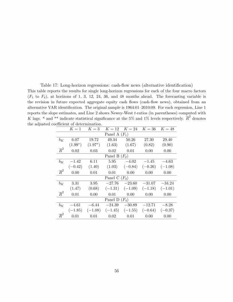
Table 17: Long-horizon regressions: cash-flow news (alternative identification)This table reports the results for single long-horizon regressions for each of the four macro factors

(F1 to F4), at horizons of 1, 3, 12, 24, 36, and 48 months ahead. The forecasting variable is

the revision in future expected aggregate equity cash flows (cash-flow news), obtained from an

alternative VAR identification. The original sample is 1964:01–2010:09. For each regression, Line 1

reports the slope estimates, and Line 2 shows Newey-West t-ratios (in parentheses) computed with

K lags. * and ** indicate statistical significance at the 5% and 1% levels respectively. R2

denotes

the adjusted coefficient of determination.K = 1 K = 3 K = 12 K = 24 K = 36 K = 48

Panel A (F1)

bK 6.07 19.72 49.34 50.26 27.30 29.40(1.99∗) (1.97∗) (1.63) (1.67) (0.82) (0.90)

R2

0.02 0.03 0.02 0.01 0.00 0.00

Panel B (F2)

bK −1.42 6.11 5.95 −4.02 −1.45 −4.63(−0.42) (1.40) (1.03) (−0.84) (−0.26) (−1.08)

R2

0.00 0.01 0.01 0.00 0.00 0.00

Panel C (F3)

bK 3.31 3.95 −27.76 −23.60 −31.07 −34.24(1.47) (0.68) (−1.31) (−1.09) (−1.18) (−1.01)

R2

0.01 0.00 0.01 0.00 0.00 0.00

Panel D (F4)

bK −4.61 −6.44 −24.39 −30.89 −12.71 −8.28(−1.85) (−1.08) (−1.45) (−1.55) (−0.64) (−0.37)

R2

0.01 0.01 0.02 0.01 0.00 0.00

56

Panel A (CSMB) Panel B (CHML)

Panel C (CUMD) Panel D (CLIQ)

Figure 1: Equity risk factorsThis figure plots the time-series for the 60-month rolling sum of the equity risk

factors. The variables are the liquidity factor (CLIQ); size factor (CSMB);

value factor (CHML); and momentum factor (CUMD). The sample period

is 1964:01–2010:09. The vertical lines indicate the NBER recession periods.

57