Effect of Pavement Conditions on Rolling Resistance and Fuel Consumption Karim Chatti, Ph.D. Department of Civil & Environmental Engineering Michigan State University East Lansing, MI 48824 Pavement Life Cycle Assessment Workshop University of California, Davis Davis, California May 5-7, 2010
Transcript
Effect of Pavement Conditions on Rolling
Resistance and Fuel Consumption
Karim Chatti, Ph.D.
Department of Civil & Environmental Engineering
Michigan State University
East Lansing, MI 48824
Pavement Life Cycle Assessment Workshop
University of California, Davis
Davis, California
May 5-7, 2010
What do we mean by driving
resistance and rolling resistance?
• air resistance
• rolling resistance
• inertial resistance
• gradient resistance
• side force resistance
• transmission losses
• losses from the use of auxiliaries
• engine friction
2
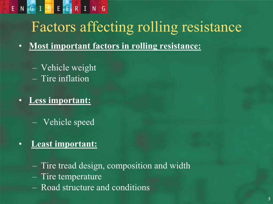
Factors affecting rolling resistance• Most important factors in rolling resistance:
– Vehicle weight
– Tire inflation
• Less important:
– Vehicle speed
• Least important:
– Tire tread design, composition and width
– Tire temperature
– Road structure and conditions3
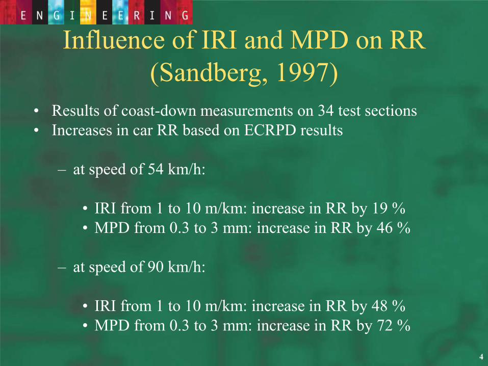
Influence of IRI and MPD on RR
(Sandberg, 1997)
• Results of coast-down measurements on 34 test sections
• Increases in car RR based on ECRPD results
– at speed of 54 km/h:
• IRI from 1 to 10 m/km: increase in RR by 19 %
• MPD from 0.3 to 3 mm: increase in RR by 46 %
– at speed of 90 km/h:
• IRI from 1 to 10 m/km: increase in RR by 48 %
• MPD from 0.3 to 3 mm: increase in RR by 72 %
4
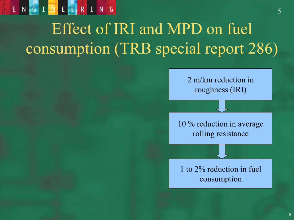
Effect of IRI and MPD on fuel
consumption (TRB special report 286)
2 m/km reduction in
roughness (IRI)
10 % reduction in average
rolling resistance
1 to 2% reduction in fuel
consumption
5
5
Gaps in knowledge
• The understanding of the relationship
between pavement surface characteristics
and vehicle fuel consumption is still in
development.
• Current models require improvement.
6
NCHRP 1-45 : Effect of pavement
conditions on fuel consumption
• Recommend models for estimating the effects of
pavement surface condition on VOC. These
models should be able to:
a) Take into account pavement, traffic and
environmental conditions encountered in the US
b) Address the full range of vehicle types
7
United States VOC Models
Development
Winfrey,
Claffey
1968-1971
Intermediate
Brazil Study
1975-1980
US Data on
1970's Vehicle
France Price
Indexing
1976
Red Book
AASHTO
1978
TRDF VOC Model
1982
MicroBENCOST
VOC
1991-1992
Canada: HUBAM
Alberta
United States:
HIAP
HPMS
HERS
State DOT
FHWA
State DOT
Counties
Municipalities
8
8
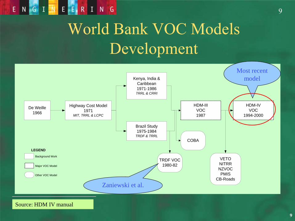
De Weille
1966
Highway Cost Model
1971MIT, TRRL & LCPC
Kenya, India &
Caribbean
1971-1986TRRL & CRRI
Brazil Study
1975-1984TRDF & TRRL
HDM-III
VOC
1987
HDM-IV
VOC
1994-2000
TRDF VOC
1980-82
COBA
VETO
NITRR
NZVOC
PMIS
CB-Roads
Background Work
LEGEND
Major VOC Model
Other VOC Model
World Bank VOC Models
Development
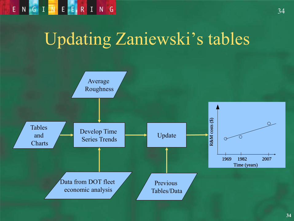
Zaniewski et al.
Most recent
model
Source: HDM IV manual
9
9
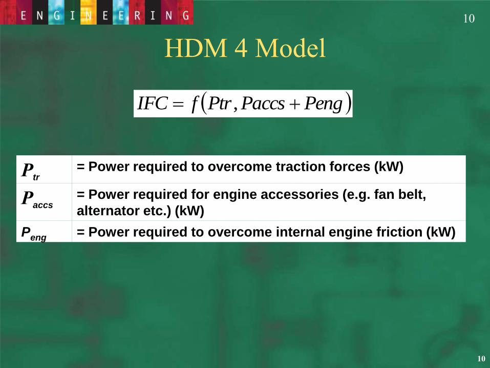
HDM 4 Model
PengPaccsPtrfIFC ,
Ptr= Power required to overcome traction forces (kW)
Paccs= Power required for engine accessories (e.g. fan belt,
alternator etc.) (kW)
Peng = Power required to overcome internal engine friction (kW)
10
10
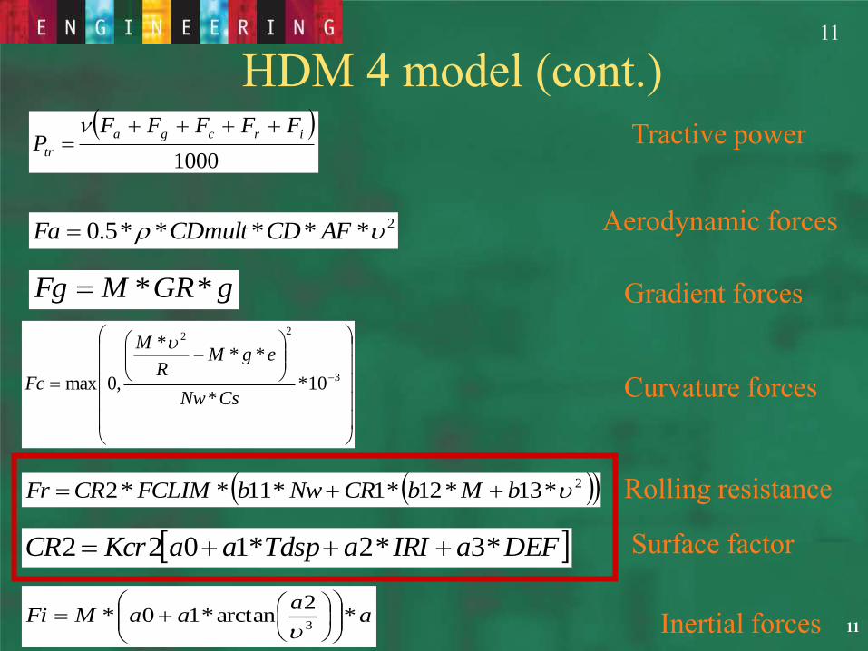
HDM 4 model (cont.)
Aerodynamic forces
Rolling resistance
Gradient forces
Curvature forces
Inertial forces
1000
ircga
tr
FFFFFP
2*****5.0 AFCDCDmultFa
gGRMFg **
3
22
10**
***
,0maxCsNw
egMR
M
Fc
2*13*12*1*11**2 bMbCRNwbFCLIMCRFr
aa
aaMFi *2
arctan*10*3
Tractive power
DEFaIRIaTdspaaKcrCR *3*2*1022 Surface factor
11
11
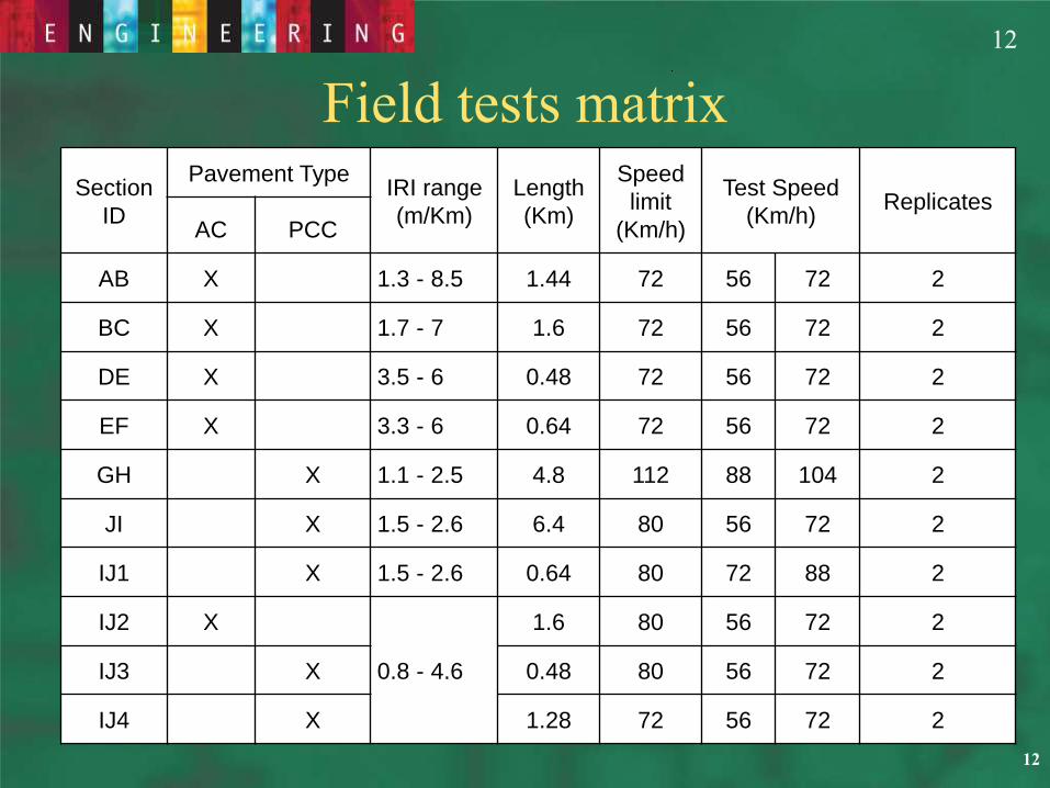
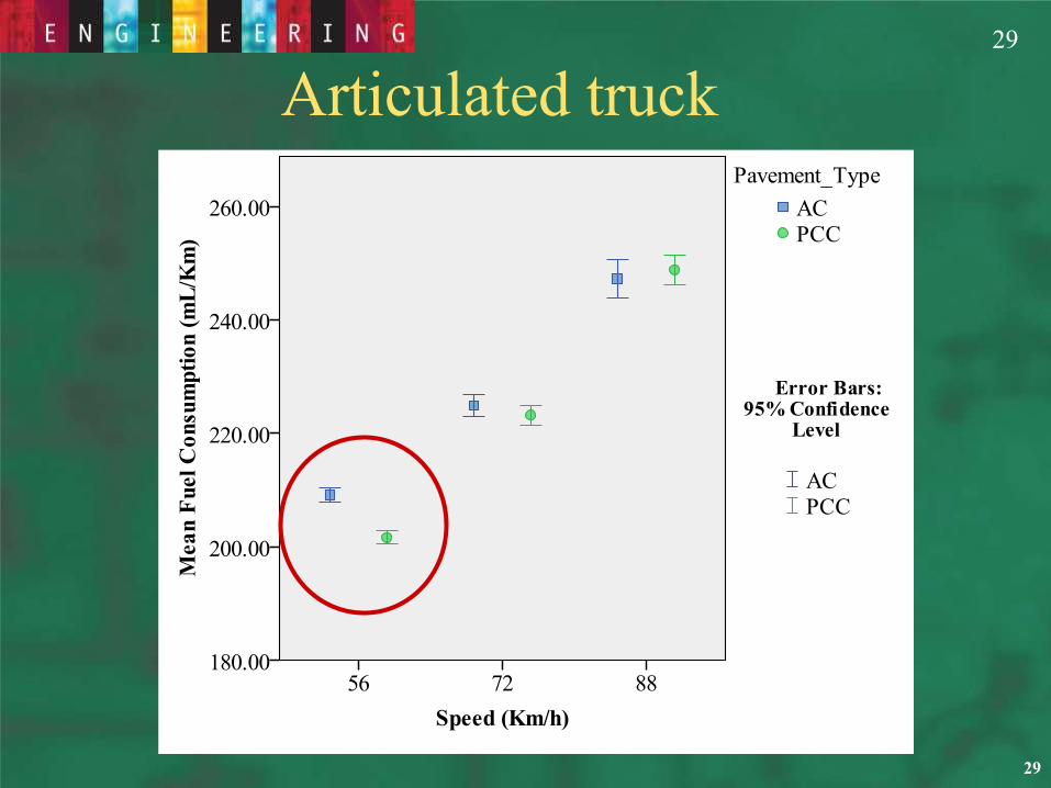
Field tests matrix
Section
ID
Pavement TypeIRI range
(m/Km)
Length
(Km)
Speed
limit
(Km/h)
Test Speed
(Km/h)Replicates
AC PCC
AB X 1.3 - 8.5 1.44 72 56 72 2
BC X 1.7 - 7 1.6 72 56 72 2
DE X 3.5 - 6 0.48 72 56 72 2
EF X 3.3 - 6 0.64 72 56 72 2
GH X 1.1 - 2.5 4.8 112 88 104 2
JI X 1.5 - 2.6 6.4 80 56 72 2
IJ1 X 1.5 - 2.6 0.64 80 72 88 2
IJ2 X
0.8 - 4.6
1.6 80 56 72 2
IJ3 X 0.48 80 56 72 2
IJ4 X 1.28 72 56 72 2
12
12
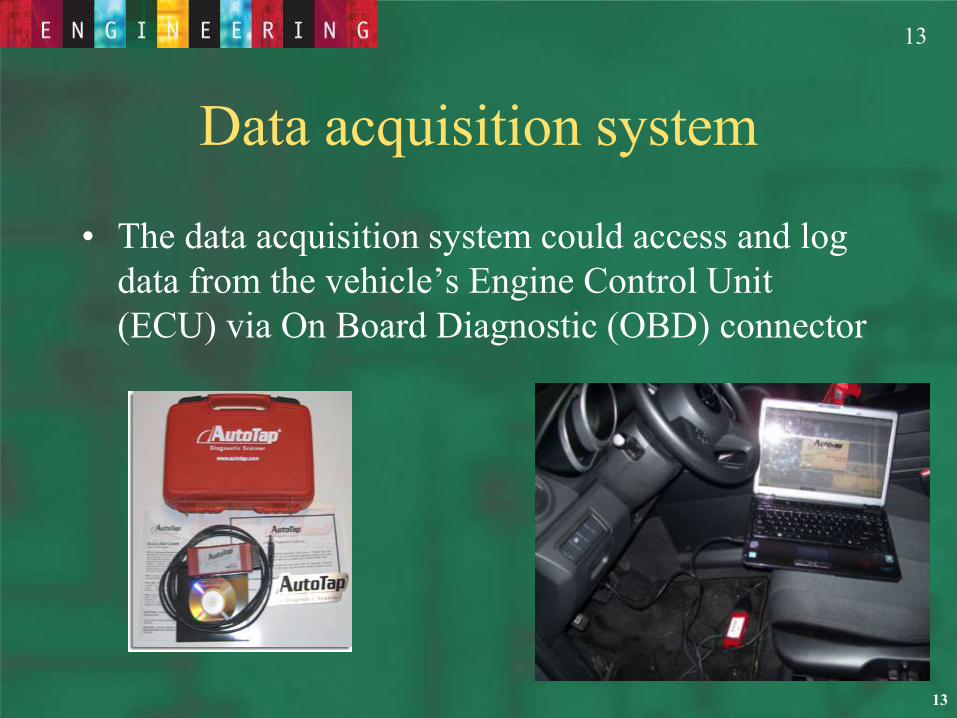
Data acquisition system
• The data acquisition system could access and log
data from the vehicle’s Engine Control Unit
(ECU) via On Board Diagnostic (OBD) connector
13
13
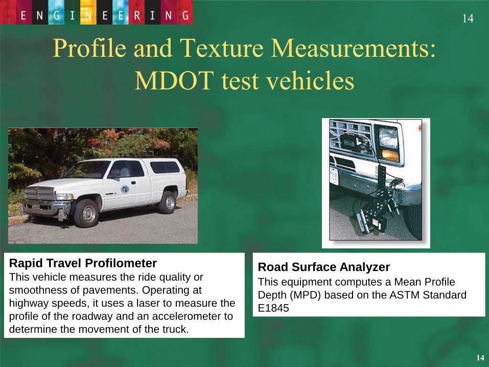
Profile and Texture Measurements:
MDOT test vehicles
Road Surface Analyzer
This equipment computes a Mean Profile
Depth (MPD) based on the ASTM Standard
E1845
Rapid Travel ProfilometerThis vehicle measures the ride quality or
smoothness of pavements. Operating at
highway speeds, it uses a laser to measure the
profile of the roadway and an accelerometer to
determine the movement of the truck.
14
14
Slope surveys: High Precision GPS
• The sampling rate is every 1 second
at highway speed (every 100ft).
• The average error is 0.5 inch per
0.3 miles,
15
15
16
16
Loading conditions
Light truck Heavy truck
6,210 lb 47,000 lb
17
17
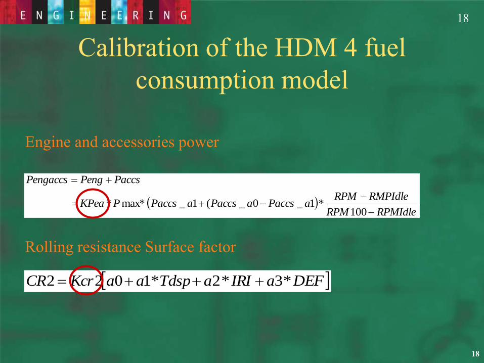
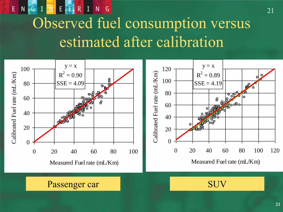
Calibration of the HDM 4 fuel
consumption model
RPMIdleRPM
RMPIdleRPMaPaccsaPaccsaPaccsPKPea
PaccsPengPengaccs
100*1_0_(1_max**
DEFaIRIaTdspaaKcrCR *3*2*1022
Rolling resistance Surface factor
Engine and accessories power
18
18
Effect of engine speed prediction errors
on the calibration
0
500
1000
1500
2000
2500
0 20 40 60 80Speed (Km/h)
Engin
e sp
eed (
rpm
)
measured engine speed
engine speed model (HDM 4)
Overestimation of the engine
speed
Overestimation of the engine
and accessories power
Underestimation of the
traction power
=
Underestimation of the effect
of pavement conditions
19
19
Calibration of the HDM 4 engine
speed model
0
500
1000
1500
2000
0 500 1000 1500 2000
Measured Engine Speed (rpm)
Pre
dic
ted
En
gin
e S
pee
d (
rpm
) .
Van
y = 0.0062x3 - 0.3018x
2 + 6.7795x + 671.98
R2 = 0.96
0
500
1000
1500
2000
2500
0 20 40 60Speed (Km/h)
En
gin
e sp
eed
(rp
m)
measured engine speed-Wet conditionengine speed model (HDM 4)measured engine speed-Dry conditionCalibrated model