PB-219 754 David B. McWhorter Colorado State …pdf.usaid.gov/pdf_docs/PNAAA055.pdfPB-219 754 STEADY...

PB-219 754

STEADY AND UNSTEADY FLOW OF FRESH WATER IN SALINE AQUIFERS

David B McWhorter

Colorado State University

Prepared for

Agency for International Development

June 1972

DISTRIBUTED BY

Naiuel Technical Infonation Service USDEPAITMNT OF COMMERCE 5285 Port Royal Road Springfield Va 22151

- -

CM UNS bullFM -COLORADO-

ri GWAER MANAGEMENTTEHNCA REPORTNO 20 -41Mshy

STEADY AND UNSTEADY FLOW OF FRESH WATER

IN SALINE AQUIFERS

Water Management Technical Report No 20

by

David B McWhorter

Pripare- under support of

United States Agency for International Development Contract No AIDcsd-2162

Water Management Research in Arid and Sub-Humid Lands of the

Less Developed Countries

180


Fort Collins Colorado

June 1972

AER71-72DBM27

______

-] w b + 7-bull - - 5 - ________ bull+ W U

Steady and Unsteady Flow of Fresh Water in Saline Aquifers

David B McWhorter

P j 931 -17-1-489--- Colorado State Unive bull

tEngineering Research Center Io G -- p ---- C AIDcsd-2162

COvered Technical 68 - i71Department of State - 6

Agency for International Development Washington DC 20523

1 6 Abieat

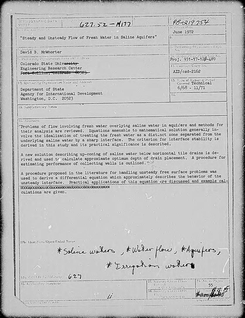
gtProblems of flow involving fresh water overlying saline waterinaquifers and methods for

their analysis are reviewed Equations amenable to mathematical solution generally inshy

volve the idealization of treating the fresh water as a distinct zone separated from the

underlying saline water by a sharp interface The criterion for interface stability is

derived in this study and its practical significance is described

A new solution describing up-coning of saline water below horizontal tile drains is de-A procedure forrived and used tr~calcuiate approximate optimum depth of drain placement

estimating performance of collecting wells is outlined V)

A procedure proposed in the literature for handling unsteady free surface problems was

used to derive a differential equation which approximately describes the behavior of the

unsteady intqrface Practical applications of this equationgtre discussed and example calshy

culations are given

AA

17b fl uni-esiOpe nFndedTe i r 2 Ji+ I

1T

l - (This 21-

j i C

J+ _____ _+4 +_ _ - T ___ ~L- 4

IL K ~ r3~ ~2

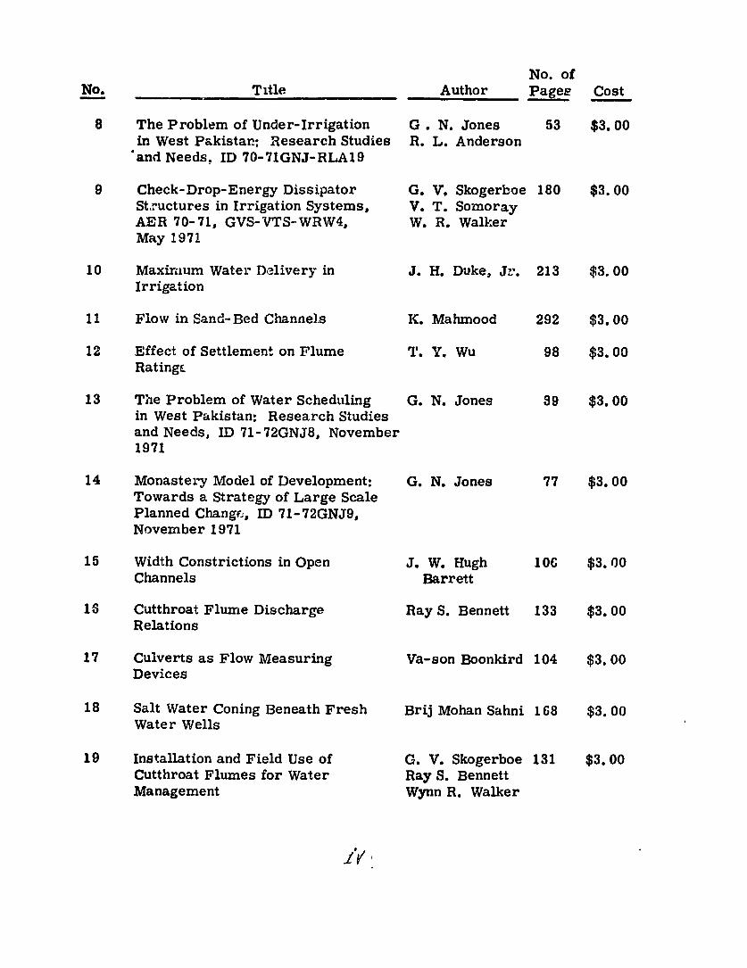
Reports published previously in this s ries are listed below Copies can be obtained by contacting Mrs Mary Fox Engineering Research Center Colorado State University Fort Collins Colorado 80521 The prices noted are effective as long as supplies last After the supply of reports is exhausted xerox copies can be provided at 10 cents per page

No of No Title Author Pages Cost

1 Bibliography with Annotations on K Mahrmood 165 $300 Water Diversion Conveyance and A G Mercer Application for Irrigation and E V Richardson Drainage CER69-70KgtT3 Sept 69

2 Organization of Water Management P 0 Foss 148 $300 for Agricultural Production in J A Straayer West Pakistan (a Progress Report) R Dildine ID70-71-1 May 1970 A Dwyer

R Schmidt

3 Dye Dilution Method of Discharge W S Liang 36 $300 Measurement CER70-71WSL- E V Richardson EVR47 January 1971

4 Water Management in West Robert Schmidt 167 $3JO Pakistan MISC-T-70-71RFS43 May 1970

5 The Economics oplusmn Water Use An Debebe Worku 176 $3 00 Inquiry into the Economic Beshyhavior of Farmers in West Pakistan MISC-D-70-71DW44 March 1971

6 Pakistan Government and Garth N Jones 114 $300 Administration A Compreshyhensive Bibliography ID70-71GNJ17 March 1971

7 The Effect of Data Limitations Luis E 225 $300 on the Application of Systems Garcia-Martinez Analysis to Water Resources Planning in Developing Countries CED70-71LG35 May 1971

U

No Title Author No of Pagee Cost

8 The Problem of Under-Irrigation in West Pakistan Research Studies and Needs ID 70-71GNJ-RLA19

G R

N Jones L Anderson

53 $300

9 Check-Drop-Energy Dissipator Structures in Irrigation Systems AER 70-71 GVS-VTS-WRW4 May 1971

G V Skogerboe V T Somoray W R Walker

180 $300

10 Maximum Water Delivery in Irrigation

J H Duke Jr 213 $300

11 Flow in Sand-Bed Channels K Mahmood 292 $300

12 Effect of Settlement on Flume Rating

T Y Wu 98 $300

13 The Problem of Water Scheduling in West Pakistan Research Studies and Needs ID 71-72GNJ8 November 1971

G N Jones 39 $300

14 Monastery Model of Development Towards a Strategy of Large Scale Planned Changre ID 71-72GNJ9 November 1971

G N Jones 77 $300

15 Width Constrictions in Open Channels

J W Hugh Barrett

106 $300

1 Cutthroat Flume Discharge Relations

Ray S Bennett 133 $300

17 Culverts as Flow Measuring Devices

Va-son Boonkird 104 $300

18 Salt Water Coning Beneath Fresh Water Wells

Brij Mohan Sahni 168 $300

19 Installation and Field Use of Cutthroat Flumes for Water Management

G V Skogerboe Ray S Bennett Wynn R Walker

131 $300

TABLE OF CONTENTS

SUMMARY 1

INTRODUCTION

PROBLEM FORMULATION

3

4

Miscible Flow Formulation

Immiscible Flow Formulation 7

Free Surface Problems 8

9Conditions on the Interface

12SOLUTIONS FOR STEADY UPCONING BENEATH WELLS

Muskat and Wyckoff 12

Bear and Dagan 15

Wang 16

17McWhorter

Other Solutions

19

SOLlION FOR STEADY UPCONING BENEATH DRAINS 20

SOLUTION FOR STEADY UPCONING BENEATH COLLECTOR WELLS 26

UNSTEADY UPCONING BENEATH WELLS 27

PRACTICAL CONSIDERATIONS 30

3SFUTURE WORK

36References

APPENDICES

A - DERIVATION OF THE DIFFERENTIAL EQUATION FOR UNSTEADY FLOW TO

SKIMMING WELLS 40

DRAIN DEPTH 46B - EXAMPLE CALCULATION FOR OPTIMUM

48C - EXAMPLE CALCULATION USING UNSTEADY FORMULA

I

SUMMARY

This report presents a relatively detailed review of the methods

that have been reported in the literature for analyzing problems of flow

in aquifers that are saturated with a zone of relatively fresh water

which becomes increasingly saline with depLh The equations which

describe the problem as one of flow of miscible fluids are presented

and discussed It is pointed out that difficulty of obtaining solutions

to these equations has fostered numerous attempts to obtain solutions

to a more idealized version of the problem The idealization consists

of treating the fresh water as a distinct zone separated from the undershy

lying saline water by a sharp interface The principle difficulty with

the latter formulation is a non-linear boundary condition on the intershy

face between the two zones

The conditions at the interface are discussed in detail It is

shown that interface is unstable under certain conditions The criterion

for interface stability is derived and its practical significance disshy

cussed

Various solutions for steady up-coning beneath wells are presented

and their limitations discussed A new solution to the problem of

steady up-coning beneath horizontal tile drains is derived in this

report It is shown how this solution can be used to calculate the

approximate optimum depth to which drains should be placed Example

calculations are given in the appendix A procedure for estimating the

performance of collector wells is discussed briefly

A procedure for handling unsteady free-surface problems previously

proposed in the literature was used to derive a differential equation

which approximately describes the behavior of the unsteady interface

- Ishy

2

Some practical applications of this equation are discussed and example

calculations given

Finally some needs for future research are outlined

3

INTRODUCTION

Exploitation of groundwater supplies for agricultural municipal

and industrial uses is severely hampered in many regions of the world

by the encroachment of unuseable saline water in response to fresh water

withdrawals Examples of salt water encroachment are most numerous in

coastal aquifers but sometimes presents a problem in inland aquifers as

well Probably the most important example of the latter case exists in

the India-Pakistan subcontinent in the Indus River Basin

Pakistan has an area of almost 200 million acres over 30 million

acres of which is irrigated The irrigated area is laced with thousands

of miles of canals and ditches used to supply farmers with essential

irrigation water Seepage for the extensive distribution system and

deep percolation from precipitation and irrigation over the years has

in many areas produced a high water table in the underlying alluvial

aquifer The high water table has caused wide-spread problems ef watershy

logging and salinity necessitating the installation of extensive drainshy

age and reclamation programs (15 33)

The problem of drainage is complicated by the fact that highly

saline watro underlies virtually all of the relatively fresh water

throughout the aquifer Near the rivers and canals uhere a supply of

fresh surface water is available the saline water exists only at great

Near the center of the doabs between the major tributaries todepths

the Indus a zone of relatively fresh water less than 100 feet thick

commonly overlies a zone of more highly saline water (9) In such areas

drainage facilities are apt to draw a substantial portion of their disshy

charge from the saline zone unless special care is taken The disposal

of the saline water produced by such facilities presents a major problem

4

In many cases the saline water can be discharged into nearby canals or

otherwise mixed with canal water and used for irrigation This procedure

can only constitute a short term solution to the problem however This

fact coupled with the need for supplemental irrigation water provides

substantial incentive to skim the fresh water from the aquifer with

a minimum disturbance of the saline zone

Research was underLaken to examine the various methods by which

skimming can be accomplished A dissertation entitled Salt-Water

Coni ag Beneath Fresh-Water Wells by B M Sahni (29) presents the

results of efforts to improve the design of shallow tubewells constructed

for skimming purposes This paper presents a review of several of the

methods for analyzing fresh-salt water interface problems as well as

reporting on a portion of the research dealing with the design of horizonshy

tal drains Another purpose of this paper is to report the development

of a procedure for estimating the behavior of the interface between

fresh and salt water under unsteady flow conditions The formulation

of the unsteady state problem is totally untested at the present but

should provide relatively satisfactory engineering answers when used

with caution Some examples of possible applications of the unsteady

state equation are presented

PROBLEM FORMULATION

The complexity of the phenomenon of flow of fresh water underlain

by brine has led investigators to make numerous idealizations in attempts

to reduce the mathematical description of the phenomenon to a tractable

form A very common practice is to regard the fresh water and brine as

In realityimmiscible liquids with an abrupt interface between them

5

the two liquids are miscible and a transition zone separates the brine

and the fresh water The transition zone is characterized by a continushy

ous decrease of concentration of salt from that of the undiluted brine

to that of the uncontaminated water above A mathematical formulamption

which considers the fluids to ba miscible is more realistic but less

tractable than one which considers the liquids to be immiscible Both

formulatiois are important however and are discussed in some detail

in the following paragraphs

Miscible Flow Formuiation

Any discussion of the flow of miscible fluids in porous media requires

consideration of hydrodynamic dispersion Hydrodynamic dispersion is

the name given the process by which a contaminant becomes mixed and

distributed in a porous medium as the result of velocity distributions

and fluctuations and molecular diffusion on a pore-size scale Mathematical

characterization of the phenomenon has required consideration of contaminshy

ant transport at the pore-size (microscopic) scale and the development

of an averaging procedure by which the microscopic mechanisms can be

expressed in macrosocopic terms which are observable and measureable

The result is the following equation known as the differential equation

)f hydrodynamic dispersion

ac a Ic e

a xDi j ax - ()

in which

c = contaminant concentration - ML3

t = time - T

x = i th cartesian coordinate - L 1

6

= coefficient of hydrodynamic dispersion (atensor of

rank 2) - L2T

i th direction shyv = the component of seepage velocity in the

LT

S1 = source or sink - ML3 T

Several analytic solutions of the above equation exist under a

variety of boundary and initial conditions and with different formulations

The analytic solshyof the source-sink term (5 13 17 18 23 24 25)

utions have contributed greatly to the understanding of hydrodynamic

dispersion and their importance cannot be over emphasized However the

analytic solutions are ordinarily derived for boundary and initial condishy

tions that are relatively simple in comparison to the wide variety of

situations encountered in the field

Numerical solutions using finite difference formulations and the

finite element method have also been developed (28 22) Numerical

solutions are usually more general in as much as complex boundary and

initial conditions can be handled for dispersion in non-isotropic and

-Numerical solutions are ordinarily lessnon-homogeneous porous media

convenient for analysis and design than are analytical solutions In

many cases however numerical methods offer the only feasible means of

solving the problem

Becauss the seepage velocity vi is present in equation 1 and

because the coefficient of hydrodynamic dispersion Di j depends on vi

the phenomenon of dispersion is strongly dependent upon the flow of the

To some extent the bulk flow of the solution phase is solution phase

also dependent on the concentration distribution of the contaminant

This is true because the contaminant effects the density and viscosity

7

of the solution The differential equation for flow including the influshy

ence of the contaminant can be written as in equation 2

pkxi ag ) ] + S 2)

1 1 1

where

L2kxi = intrinsic permeability in the xi direction -

P = pressure - FL2

2 g = gravitational constant - LT

h = elevation with respect to an arbitrary datum - L

P = density - ML3

p = dynamic viscosity - FTL2

0 = porosity

S2 = source or sink - ML3T

and other symbols are as previously defined Equations 1 and 2 constitute

a system of non-linear coupled partial differential equations which

describe bulk flow of a liquid and dispersion of a contaminant in that

liquid

Immiscible Flow Formulation

One of the objectives of the study reported herein is to provide

a method for comparing different methods of producing the relatively

fresh water with a minimum disturbance of the underlying brine From

an academic standpoint the ideal way to accomplish such a comparison

would be to solve equations 1 and 2 simultaneously for each method under

consideration Because of limitations on time and financial recources

such a procedure is quite impractical Therefore a less rigorous but

8

This approach involves severalmore practical approach was taken

idealizations which are discussed in the following paragraphs

It is often the case that the disperse (or transition) zone between

the fresh-water region and the salt-water region is small compared to

the total thickness of the fresh-water region It is therefore possible

to consider the transition zone as a sharp boundary separating the two

The problem is reduced to locating the interface betweenregions of flow

the two regions for various boundary conditions which is often called a

free-surface problem

Free Surface Problems

Within each region separated by the abrupt interface the flow is

given by Darcys law in vector notation for isotropic media

(3)qf = - KfV (PfYf + z)

(4)qs = - KsV (PsYs + z)

inwhich

q = Darcy velocity vector - LT

K = hydraulic conductivity - LT

P = pressure - FL2

-z = elevation relative to an arbitrary datum L

- FL3 y = specific weight

refer to fresh and salt water respectivelyand the subscripts f and s

Through-The quantity in parathenses is often called the hydraulic head

out the remainder of this report the hydraulic head is denoted by the

symbol H For a homogeneous medium equation 3 can be combined with

9

the equation for mass conservation for incompressible homogeneous fluids

to obtain

V2Hf= 0 bull (5)

The same equation applies to the salt-water region with the subscript

Equation 5 is known as the Laplace equation Thef replaced by s

hydraulic head Hf is a function of space and time in general

The problem is to solve the linear Laplace equation in the fresh

water region subject to the boundary conditions Dagan (6) has shown

that the problem represented by equation 5 within a region whose boundary

is partially a free surface is non-linear because of a non-linear boundshy

ary condition on the interface The non-linear boundary condition conshy

stitutes the major difficulty with the immiscible formulation of the

problem

Conditions on the Interface

At any point the pressure must be continuous across the interface

Therefore solving for pressure from the definitions of hydraulic head

in the fresh and salt water regions and equating at the interface yields

H i y yf S- Eys (6)

in which C is the vertical coordinate of the interface at any point

denotes the value of hydraulic head on the interfacethe superscript i

and other symbols are as pr3viously defined

10

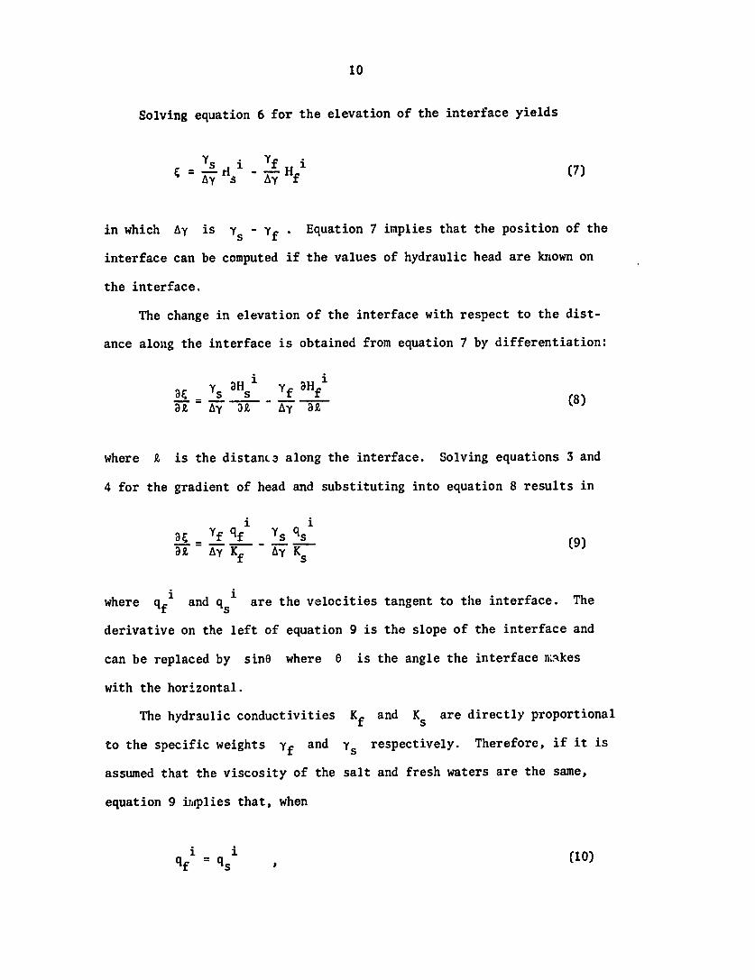
Solving equation 6 for the elevation of the interface yields

s d i Yf 1 = s - Hf 7)

in which Ay is ys- Yf Equation 7 implies that the position of the

interface can be computed if the values of hydraulic head are known on

the interface

The change in elevation of the interface with respect to the distshy

ance along the interface is obtained from equation 7 by differentiation

i Hi

Sys 3Hs Yf 3Hf at A A(y 8)

where k is the distana along the interface Solving equations 3 and

4 for the gradient of head and substituting into equation 8 results in

DE _ f qf YS q s (9)ii

where qf and qs are the velocities tangent to the interface The

derivative on the left of equation 9 is the slope of the interface and

can be replaced by sine where 0 is the angle the interface nAkes

with the horizontal

The hydraulic conductivities Kf and Ks are directly proportional

to the specific weights Yf and ys respectively Therefore if it is

assumed that the viscosity of the salt and fresh waters are the same

equation 9 implies that when

qf = qs P (10)

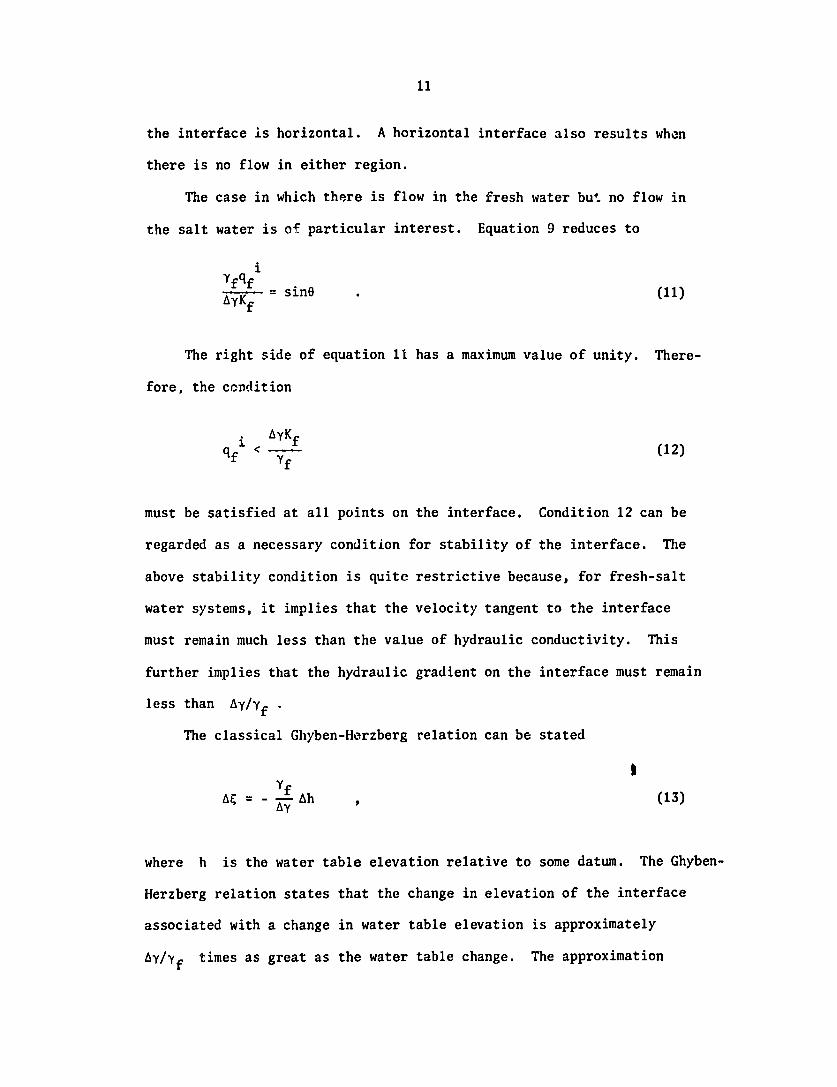
11

the interface is horizontal A horizontal interface also results when

there is no flow in either region

The case in which there is flow in the fresh water but no flow in

the salt water is of particular interest Equation 9 reduces to

i yfqf

AyK sin (11)

The right side of equation II has a maximum value of unity Thereshy

fore the condition

i AyKf

qf Y (12)Yf

must be satisfied at all points on the interface Condition 12 can be

regarded as a necessary condition for stability of the interface The

above stability condition is quite restrictive because for fresh-salt

water systems it implies that the velocity tangent to the interface

must remain much less than the value of hydraulic conductivity This

further implies that the hydraulic gradient on the interface must remain

less than AyYf

The classical Ghyben-Herzberg relation can be stated

Yf

A = - - Ah (13)

where h is the water table elevation relative to some datum The Ghyben-

Herzberg relation states that the change in elevation of the interface

associated with a change in water table elevation is approximately

Ayyf times as great as the water table change The approximation

12

necessary to arrive at equation 13 follows directly from equation 8 with

8H at = 0 S

ac Yf aHf(AE =UAL= y atAk (14)

or iTf

AE= - A- Hf (15)

Equation 15 is identical to the Ghyben-Herzberg relation provided the

hydraulic head on the interface is equal to the water table elevacion

Such a condition exists only if the flow is horizontal In situations

of interest in this report the flow is not horizontal because of the

slope of the interface and the water table Therefore use of the Ghyben-

Herzberg relation is tantamount to neglecting the vertical component of

flow

SOLUTIONS FOR STEADY UPCONING BENEATH WELLS

Muskat and Wyckoff

Probably the first approximate solution to the problem of upconing

beneath wells was derived by Muskat and Wyckoff (21) Their problem was

that of upconing of brine in response to pumping in the overlying oil

zone The theory does not depend upon the particular liquids involved

so the author of this report has taken the liberty of translating the

analysis into terms of the fresh water-salt water problem

Muskat and Wyckoff obtained a steady state distribution of hydraulic

head for flow toward a well partially penetratig a confined aquifer of

thickness m They then assumed that this distribution of head applies

to a situation in which thc well penetrates a fresh water zone of thickness

13

m This assumption amounts to assuming that the upconing of the saltshy

water does not disturb the flow

Explanation of the method used by Muskat and Wyckoff can be presented

in mathematical terms Let the distribution of hydraulic head be given

by

(16)Hf = Hf (rz)

z is the vertical coordinatewhere r is the radial coordinate and

An explicit expression for equation 16 is obtained as discussed in the

previous paragraph On the interface equation 16 becomes

Hf1 (17)= Hf (r )

Hfi an equation for the interface involving

two unknowns which is

Because there are two unknowns in equation 17 a second indeshyand

pendent equation is necessary The second equation is provided by the

Since interest is focused oninterface condition given by equation 7

a steady state solution the head in the salt-water zone is taken as

constant and equation 7 becomes

Yf i (18)constant - 1f

The constant in equation 18 depends upon the selection of the datum

used for measuring hydraulic head Equations 17 and 18 are a pair of

which can be solved simultaneouslyequations in the unknowns Hfi and C

to obtain the position of the interface

14

The particular form of equation 17 used by Muskat and Wyckoff made

it necessary to obtain the simultaneous solution of equations 17 and 18

by graphical methods It was found that for any particular distribution

of hydraulic head as given by equation 17 that one of the following

situations exist

1) No simultaneous solution exists

2) Two roots of the simultaneous equations exist

3) One root exists

These authors show that situation i corresponds to the physical condition

of an unstable interface that is inequality 12 is not satisfied They

further show that the only root which has physical meaning in situation

2 is the one which gives the lowest position of the interface The

third possible situation represents the highest position at which a

stable interfaco exists This position has been called the critical

cone height

Muskat and Wyckoff also present a formula for the well discharge

as calculated from the distribution of hydraulic head According to

their theory the maximum discharge is obtained when the cone height is

criticl This value of discharge has been termed the critical disshy

charge

Thus the Muskat-Wyckoff model has the advantages that the condition

of interface instability is implicit in the theory and that the vertical

component of flow is not neglected On the other hand the assumption

that the distribution of head is not effected by the upconing of the

interface is a serious constraint on the applicability of the metnod

is

Bear and Dagan

Schmorak and Mercado (30) report an equation for salt-water rise

beneath a pumping well that was derived by Bear and Dagan using the

method of small perturbations The original report of Bear and Dagan

is not in English and therefore is not used directly in this report

The equation for steady flow in a homogeneous and isotropic aquifer

is

L YfQ 1 (19)

d 21Td 2 Ay K [1+ r 2]1

in which

Q = discharge rate - L3T

r = radial distance - L

d = distance between bottom of well and the original powition

of interface - L

and other symbols are as previously defined Bear and Dagan recognized

that equation 19 does not account for the fact that the interface becomes

(t ) These authorsunstable if exceeds a certain critical value

recommend that the discharge of the well be regulated so that

(20)CM lt f d

where f is some fraction (m 05) Subject to condition 20 the

maximum safe discharge of the well is given by

r27rfd2AyK [I+(j)21] (21)Qmax - f [1(=2](1

16

where is the radius of the well These formulas were derived orrw

a very thick fresh water zone and considered the well to be a point sink

Wang

The Wang theory (32) is based on the assumption that the rising

salt-water mound beneath the pumping well does not effect the discharge

of the well In this respect the Wang theory is similar to that of

Muskat and Wyckoff The Wang theory however makes no use of a detailed

distribution of hydraulic head for locating the position of the intershy

face The approach was to use the formula presented by Muskat (20) which

relates the well discharge to drawdown and incorporates the Ghyben-

Herzberg relation The formula for discharge is

D rw2nK ms r1+ wD 2[1+7 w cos-] T (22)

Mrerw m

where

s = drawdown - L

D = distance between original water table and the bottom

of well - L

m = original fresh water thickness - L

re = radius of influence - L

Strictly speaking equation 22 applies only for flow in confined aquifers

Wang reasoned that if s is small compared to m the formula could

be used for flow in water table aquifers as well

As already pointed out the Ghyben-Herzberg equation predicts the

interface will rise yfAy feet for every foot of drawdown on the water

table (see equation 13) Therefore the elevation of the interface at

17

r = rw as a function of discharge is

QAykn rer 1w

YrnKm~yfewrjn m 1 CrO DD (2D[ 1+7 (W2 cs

Wang did not account for the possible instability of the interface

and assumed that the interface could rise to the bottom of the well as

a limiting condition This fact causes the Wang equation for maximum

discharge to be impractical It is not good for large salt-water mound

heights

McWhorter

In view of the restrictive assumptions and complicated methods by

which the above solutions were obtained the author of this report felt

that a formula that required a much simpler analysis might be useful

The major difference between the following analysis and that used in

obtaining the above equations is that the increased convergence caused

by the upconing of the interface is accounted for approximately

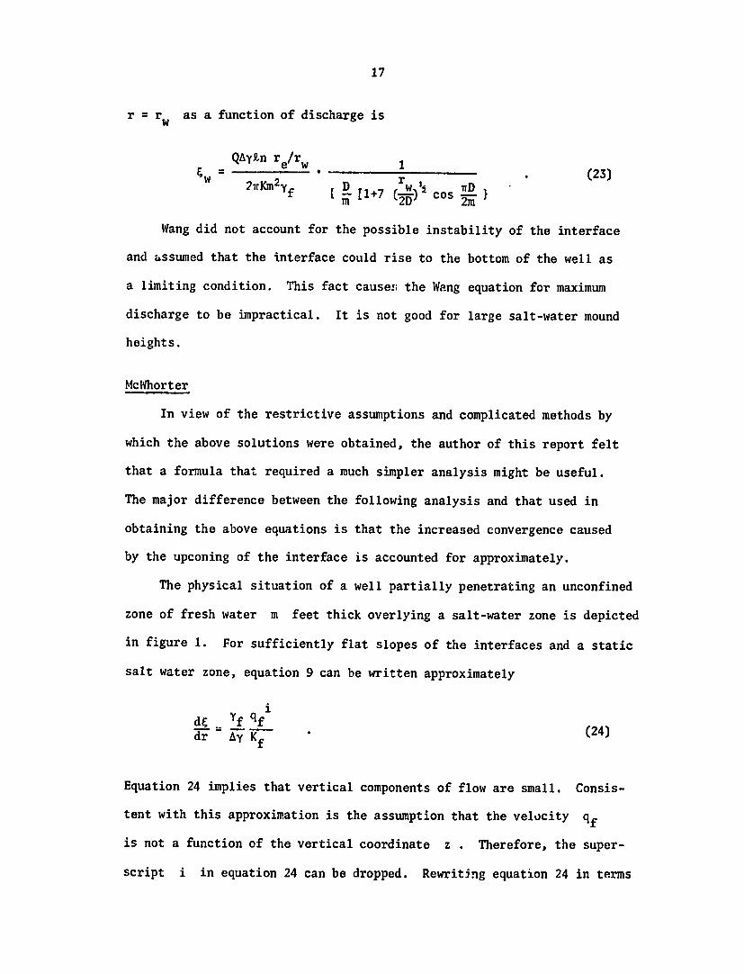
The physical situation of a well partially penetrating an unconfined

zone of fresh water m feet thick overlying a salt-water zone is depicted

in figure 1 For sufficiently flat slopes of the interfaces and a static

salt water zone equation 9 can be written approximately

i

Yf qf (24) d Ay Kf

Equation 24 implies that vertical components of flow are small Consisshy

tent with this approximation is the assumption that the velocity qf

is not a function of the vertical coordinate z Therefore the supershy

script i in equation 24 can be dropped Rewriting equation 24 in terms

18

_ original water table

7shyre shy

z d h -interface

interface

Figure 1 Upconing of salt-water beneath a pumping well

--original

of the well discharge Q results in

Q = A Ay K d (25)fYf

where A is the area perpendicular to flow and is given by

A = 2w (h-=)r (26)

The water table elevation h can be related to 9 by use of the

Ghyben-Herzberg relation which is consistent with the approximation that

vertical components of flow are small The result is

(27)A=Ayfn +1L~) r

2S u m - (7- i1t 2A = y e p n r

Substitution of equation 27 into equation 25 separation of variables

19

and integration yields

I 1Qyenfpound nrrI

)2+ - (28) mm 2AKf (l+AYYf) l+Ayyf

Equation 28 is an approximate discription of the variation of interface

elevation with r For a particular value of r say r = rw the

equation descrioes the interface elevation as a function of well disshy

charge

The derivation of equation 28 does not account for the fact that

the interface can become unstable Therefore application of equation

28 must be restricted tu the range of C values in which the interface

remains stable

Other Solutions

Bennett et al (1)used an electrical analog to obtain solutions

for the steady flow case The potential distribution in the simulated

fresh water zone was determined from the analog with a first guess as

to the shape and position of the boundary simulating the interface

The interface was then adjusted and a new potential distribution detershy

mined until the boundary conditions that must be satisfied on the intershy

face were in agreement with the potential distribution The procedure

relied heavily on the theo-ry of Muskat (20) the significant improvement

however being that the distortion of the distributlon of hydraulic

head caused by the mounding was given full consideration

Sahni (29) used both numerical and physical models to study the

design of partially penetrating wells in the fresh water zone He

developed a numerical solution by writing the differential equation in

finite difference and solving the resulting set of algebraic equations

20

The non-linear boundary condition on the interface was handled by iterashy

tion A solution was obtained with a first estimate of the position of

the interface and then the interface was adjusted until equation 7 (in

a different form) was satisfied The adjustment of the interface changes

the geometry rf the flow region and therefore a new distribution of

hydraulic head Once a new distribution of hydraulic head was determined

the interface was again adjusted This procedure was continued until

the change in the distribution of hydraulic head for a particular iterashy

tion was negligibly small Sahnis model also includes the effects of

flow in the partially saturated portion of the aquifer above the water

table

The major conclusion obtained from Sahnis work is that the optimum

penetration of the wells is between 15 and 30 ptrcent of the thickshy

ness of the fresh water zonA a much shallower penetration than was

previously recommended It was also deiionstrated by comparison with

physical model measurements that the numerical model accurately predicts

the well discharge under a variety of values for the boundary conditions

SOLUTION FOR STEADY UPCONING BENEATH DRAINS

Solutions reported in the literature for upconing beneath draiiis

are not as numerous as for the well problem Therefore as a part of

this research solutions for the drain problem were derived which parallel

solutions for the well case

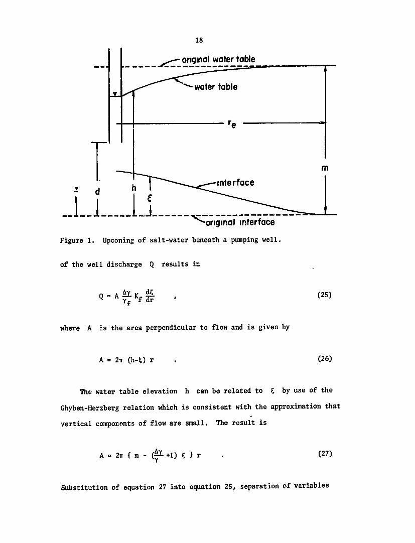
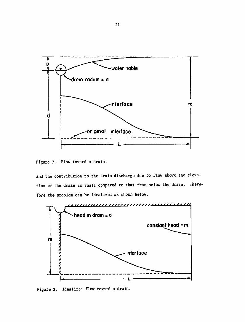
The situation treated in this report is depicted in figure 2 Flow

a disshyoccurs toward a drain of radius the center line of which isa

tance D below the original water table A constant-head boundary is

D lt lt dlocated a distance L from the drain In practical cases

21

water table

drain radius =a

interface I original interface

S-L

Figure 2 Flow toward a drain

and the contribution to the drain discharge due to flow above the elevashy

tion of the drain is small compared to that from below the drain Thereshy

fore the problem can be idealized as shown below

head indrain =d constant head =m

bull interface

-L

Figure 3 Idealized flow toward a drain

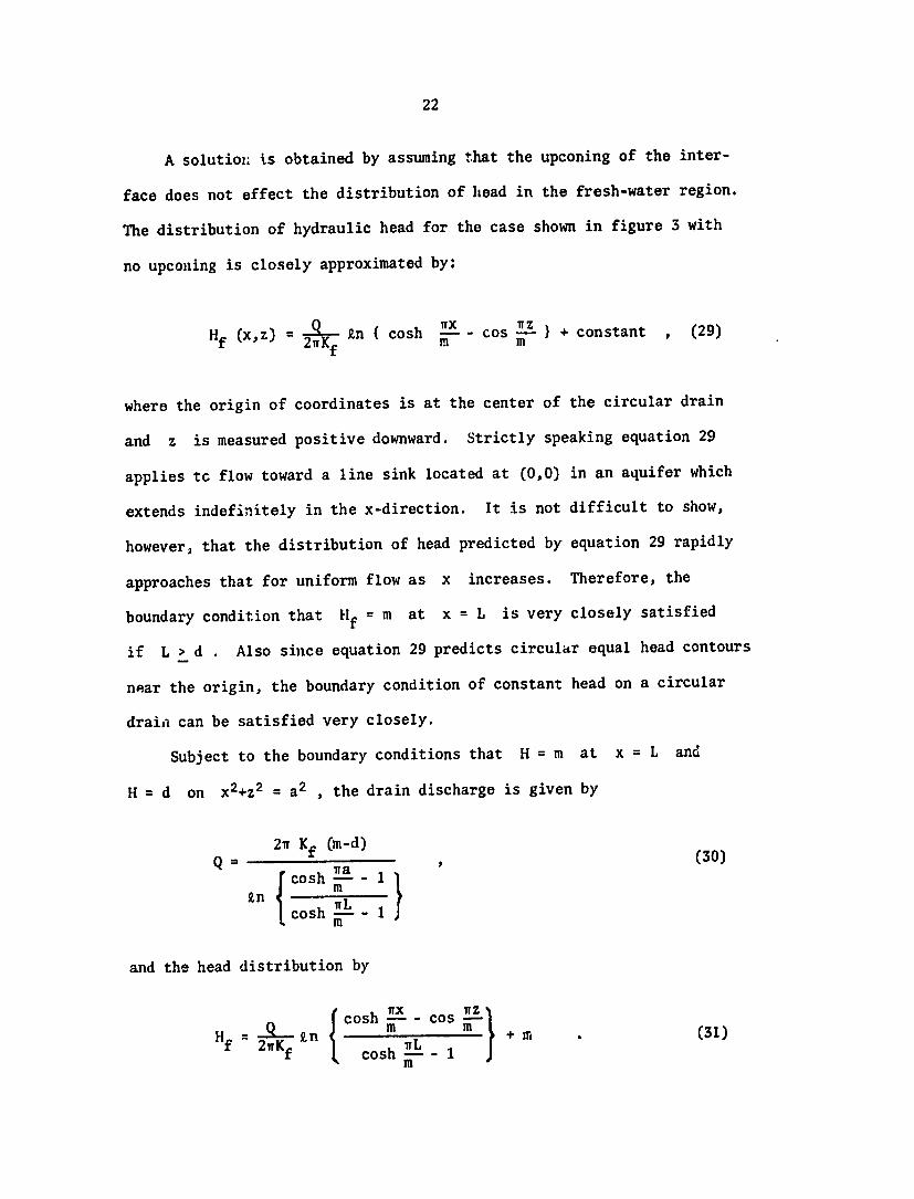
22

A solution is obtained by assuming that the upconing of the intershy

face does not effect the distribution of head in the fresh-water region

The distribution of hydraulic head for the case shown in figure 3 with

no upconing is closely approximated by

Hf (xz) = poundn ( cosh 21 - c f- + constant (29)

where the origin of coordinates is at the center of the circular drain

and z is measured positive downward Strictly speaking equation 29

applies tc flow toward a line sink located at (00) in an aquifer which

extends indefinitely in the x-direction It is not difficult to show

however that the distribution of head predicted by equation 29 rapidly

approaches that for uniform flow as x increases Therefore the

boundary condition that Hf = m at x = L is very closely satisfied

if L gt d Also since equation 29 predicts circular equal head contours

near the origin the boundary condition of constant head on a circular

drain can be satisfied very closely

Subject to the boundary conditions that H = m at x = L and

2H = d on x2+z2 = a the drain discharge is given by

27r Kf (m-d) (30)Q = co aCJcosh ITshy

mLXn

cosh--- 1

and the head distribution by

cosh n- - cos - + - -Hf f 2wKQ f 9n coshm1- 1 (31)

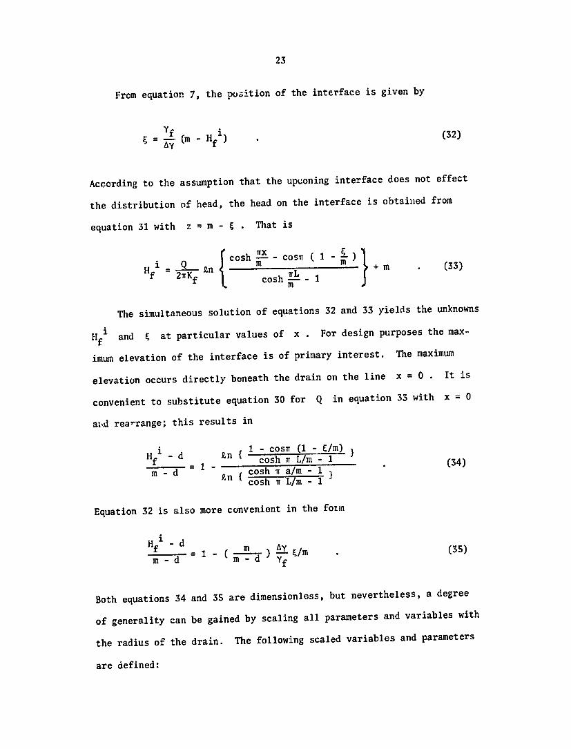
23

From equation 7 the position of the interface is given by

Yf i (32) Tf (m - Hf i )

According to the assumption that the upeoning interface does not effect

the distribution of head the head on the interface isobtained from

= m - That isequation 31 with z

- cosshycosh M

ch L 1 + M (33)2Kf m-Hf1 Q cosh L-

The simultaneous solution of equations 32 and 33 yields the unknowns

x For design purposes the max-Hf and amp at particular values of

The maximumimum elevation of the interface is of primary interest

x = 0 It iselevation occurs directly beneath the drain on the line

Q in equation 33 with x = 0convenient to substitute equation 30 for

ahd rea-range this results in

H 1 - d poundn 1- cosir (1- m) = 1 - cosh 7 Lm- 1 (34)

m - d in cosh iramshycosh TrLm - 1

Equation 32 is also more convenient in the foim

Hf - d Ay (35)

m-d = 1 - (------) fm

Both equations 34 and 35 are dimensionless but nevertheless a degree

of generality can be gained by scaling all parameters and variables with

The following scaled variables and parametersthe radius of the drain

are defined

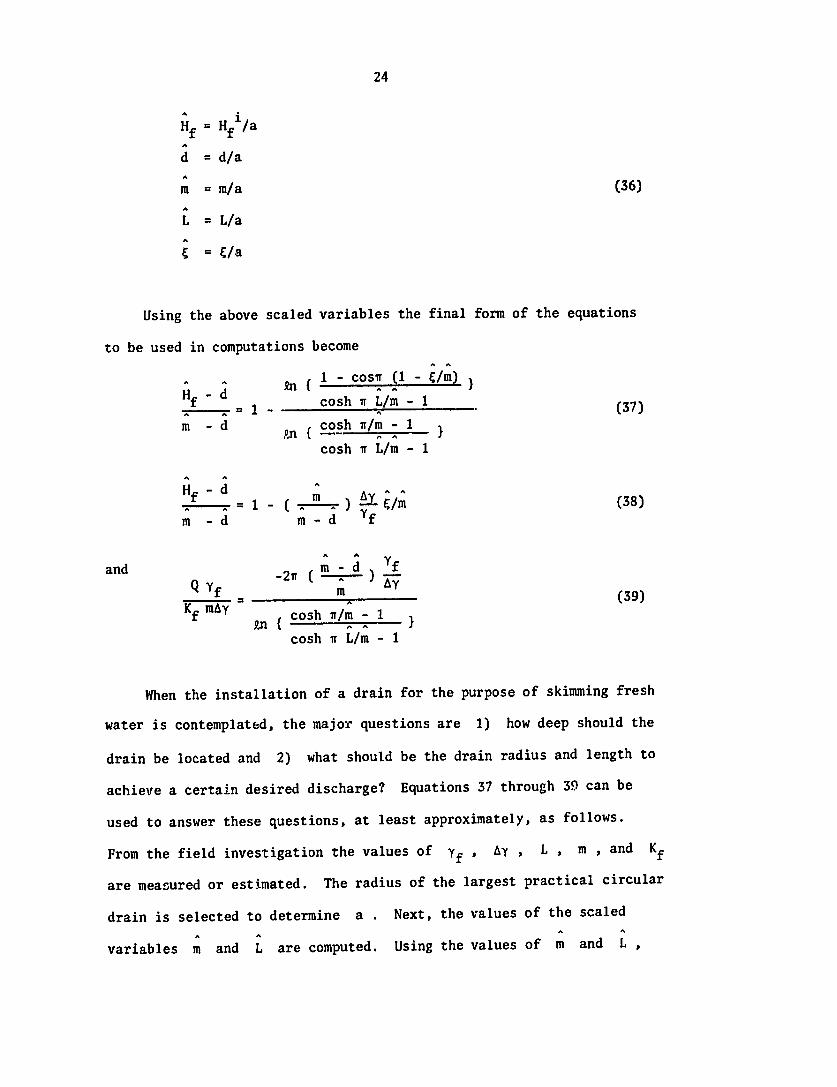
24

Hf = 1f a

d =da

m = ma (36)

L= La

Using the above scaled variables the final form of the equations

to be used in computations become

A A ~ In cosff1~) Hf d cosh w Lm - 1 (37)

m -d cosh nm^ 1

cosh ffLm - 1

Hfd d A (38)

A A

m -d m- f

and m-d YfQ m (39)-y

Kf may cosh 7rm -1

cosh n Lm - I

When the installation of a drain for the purpose of skimming fresh

water is contemplated the major questions are 1) how deep should the

drain be located and 2) what should be the drain radius and length to

achieve a certain desired discharge Equations 37 through 39 can be

used to answer these questions at least approximately as follows

From the field investigation the values of yf Ay L m and Kf

are measured or estimated The radius of the largest practical circular

drain is selected to determine a Next the values of the scaled

m and Lvariables m and L are computed Using the values of

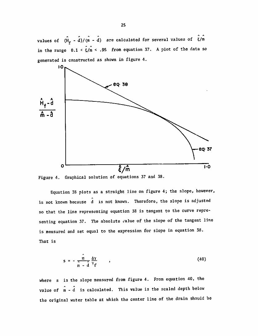
25

AA A a AA

values of (Hf - d)(m - d) are calculated for several values of Em

in the range 01 lt ampm lt 95 from equation 37 A plot of the data so

generated is constructed as shown in figure 4

10

eq 3e

A A

Hf-d

A-a

eq 37

0 00

Figure 4 Graphical solution of equations 37 and 38

Equation 38 plots as a straight line on figure 4 the slope however

is not known because d is not known Therefore the slope is adjusted

so that the line representing equation 38 is tangent to the curve represhy

senting equation 37 The absolute alue of the slope of the tangent line

is measured and set equal to the expression for slope in equation 38

That is

m Ay (40)

m-dYf

where s is the slope measured from figure 4 From equation 40 the

value of m - d is calculated This value is the scaled depth below

the original water table at which the center line of the drain should be

26

placed

The horizontal coordinate of the point of tangency in figure 4 is

the scaled height of the interface beneath the drain If the straight

line is drawn with a steeper slope the point of intersection of the

two curves represents a stable interface elevation at a drain depth less

than the one calculated above On the other hand a straight line drawn

so that there is no intersection represents a greater drain depth which

will cause an unstable interface and salt water will be entrained Thus

the tangent condition represents the greatest 3afe depth at which the

drain can be placed

The next step is to use the measured value of slope in equation 39

to compute the discharge per unit length of drain It should be pointed

out that the assumptions made in the development of the above theory are

such that the predicted discharge for a particular interface elevation

is larger than that which would be measured The descrepancy is probably

not large for thick fresh water layers but becomes larger for thin

layers An example calculation is presented in the appendix

SOLUTIONS FOR STEADY UPCONING BENEATH COLLECTOR WELLS

Collector well is the name given a collection system constructed by

lowering a vertical caisson into the aquifer sealing the bottom and

forcing perforated pipe horizontally into the formation on a radial

pattern The diameter of the caisson is ordinarily between 10 and

15 feet and the length of the laterals may be as great as 250 feet

Collector wells are expensive to construct but provide large discharges

per unit of drawdown a desirable feature of skimming facilities

27

Mathematical analysis of the yield and drawdown for collector wells

is relatively difficult because the flow is three dimensional Hantush

and Papadopulos (12) have presented an extensive analysis of flow to

A simpler but less rigorouscollector wells for a variety of cases

approach is to simulate the collector well by an equivalent vertical

Mikels and Klaer (19) report that a vertical production well withwell

90 percent of the average lateral lengthan effective radius of about

will have the some specific capacity as the collector well if the laterals

are spaced 225 degrees apart (or less) in a full circle

The assumption that a collector well can be simulated by an ordinary

081 (L= average length ofwell with an effective radius equal to

laterals) means that the formulas derived for the upconing of the intershy

face beneath wells can be used to estimate the effectiveness of collector

wells as skimming facilities by simply substituting 081 for rw in

these equations

UNSTEADY UPCONING BENEATH WELLS

an import-The time-rate of rise of the fresh-salt water interface is

ant aspect of ground water development in aquifers in which a saline zone

is present Field situations rarely exist in which the flow field is

truly steady and the optimum operation of skimming wells must certainly

depend on he rate of upconing as affected by well discharge Solutions

for steady flow while very useful for design purposes are of limited

utility in many other aspects of groundwater investigation

Unfortunately solutions to the unsteady problem are even less

Schmorak and Mercado (30)abundant than for the steady state case

report a solution for unsteady upconing in response to pumping from a

28

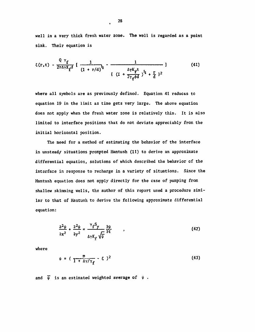
well in a very thick fresh water zone The well is regarded as a point

sink Their equation is

t(rt) QYf I1 1 (41)(1 + rd) AyKt )t r2

where all symbols are as previously defined Equation 41 reduces to

equation 19 in the limit as time gets very large The above equation

does not apply when the fresh water zone is relatively thin It is also

limited to interface positions that do not deviate appreciably from the

initial horizontal position

The need for a method of estimating the behavior of the interface

in unsteady situations prompted Hantush (11) to derive an approximate

differential equation solutions of which described the behavior of the

interface in response to recharge in a variety of situations Since the

Hantush equation does not apply directly for the case of pumping from

shallow skimming wells the author of this report used a procedure simishy

lar to that of Hantush to derive the following approximate differential

equation

D2 = _ + YfS Z (42) t

aX2 By2 AyKf a

where

m )2 (43)

and f is an estimated weighted average of 4

29

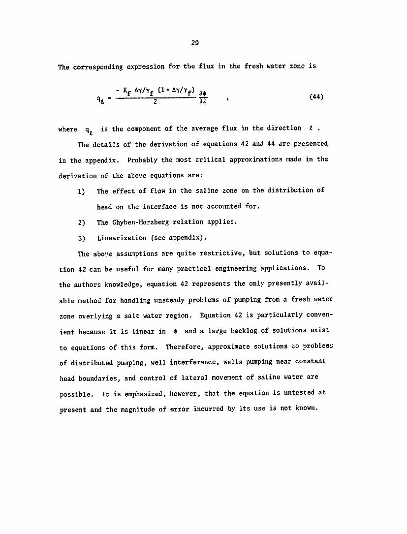
The corresponding expression for the flux in the fresh water zone is

- Kf AYYf (1+ AYYf) 34 qX = 2 a (44)

where q is the component of the average flux in the direction pound

The details of the derivation of equations 42 and 44 are presented

in the appendix Probably the most critical approximations made in the

derivation of the above equations are

1) The effect of flow in the saline zone on the distribution of

head on the interface is not accounted for

2) The Ghyben-Herzberg relation applies

3) Linearization (see appendix)

The above assumptions are quite restrictive but solutions to equashy

tion 42 can be useful for many practical engineering applications To

the authors knowledge equation 42 represents the only presently availshy

able method for handling unsteady problems of pumping from a fresh water

zone overlying a salt water region Equation 42 is particularly convenshy

ient because it is linear in $ and a large backlog of solutions exist

to equations of this form Therefore approximate solutions to problems

of distributed pumping well interference wells pumping near constant

head boundaries and control of lateral movement of saline water are

possible It is emphasized however that the equation is untested at

present and the magnitude of error incurred by its use is not known

30

PRACTICAL CONSIDERATIONS

It is virtually impossible to discuss the relation of the foregoing

theories to all of the practical problems that might be encountered In

fact the most practical solution to a particular problem will undoubtedly

involve aspects that lie far outside the scope of this report Nevertheshy

less it is instructive to discuss a few practical situations and how the

various theories in this report can be applied

One question of practical significance is that of selecting a method

of skimming the fresh water from a thin fresh-water zone The answer to

this question obviously involves consideration of factors other than the

technical Ferformance of the various facilities that might be used A

partial list of considerations other than the performance characteristics

is given below

1) Source of materials (local foreign etc)

2) Cost of construction and availability of funds

3) Impact on local employment levels

4) Impact on local manufacturers

5) Existing facilities and traditions

6) Legal

7) Technical factors such as boundary conditions or declining

water levels

The theories outlined in this report provide a method by which the

engineer can estimate the performance of various skimming facility altershy

natives He can estimate how many wells or how many feet of drain are

required to provide a given quantity of water Assuming that more than

one alternative is technically feasible the selection must be based on

considerations similar to those listed above in conference with economists

31

and other social scientists

Another important practical consideration is the operating schedules

of skimming wells For example the question of the length of time a

well can be pumped at a particular rate without running a risk of pumping

If the well is shut down what is thethe underlying salt water irises

rate of decline of the salt waser mound is another question that might

Rough answers to these questions are provided by solutions tobe asked

equation 42 as demonstrated below

A skimming ell a large distance from other wells in the area is

considered Equation 42 in radial coordinates is

32 + 1 = a (45)

Dr2 r Dr at

The boundary and initial conditions arewhere a = yfSyAyKfv

limi r9r Ay (I + Ay (46)limit r 22= r+O r Yf Yf f

2 = (-t) = m(l + AYpound))

(rO) = m(l + ATyTf)1 2 = o (47)

Q is the wellwhere m is the thickness of the fresh water zone and

discharge The solution is

(48)2i0 W(u) 27 --(1+ -) Kf

Yf Yf

32

where

(9W(U) ffr2dId~ du

4t

The function W(u) is exponential integral which is tabulated in several

standard mathematical tables

The above solution in 4 describes the time and spatial variation

of for constant well discharge The relationship of 4 to the intershy

is given by equation 43 Values of 4 (and thereforeface elevation E

t ) influenced by variable pumping rates can be estimated by applying the

principle of superpeition

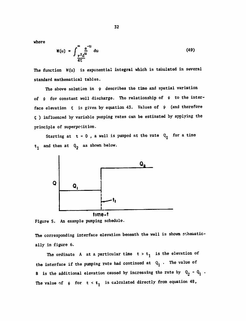
for a timeStarting at t = 0 a well is pumped at the rate

t and then at Q2 as shown below

02

I

time-t Figure S An example pumping schedule

The corresponding interface elevation beneath the well is shown sheaticshy

ally in figure 6

The ordinate A at a particular time t gt t1 is the elevation of

Q The value ofthe interface if the pumping rate had continued at

B is the additional elevation caused by increasing the rate by Q2 - Q1

The value of 0 for t lt t1 is calculated directly from equation 48

33

C(r r)

A

0 time-t

Figure 6 Schematic of the interface elevation cor-esponding to the

pumping schedule shown in figure S

is computed by -extending this solution forward in and for t gt tI

and adding to it the solution for discharge at the rate

time beyond t

t = t bull Mathematically this statement is Q2 - Q1 beginning at

In Qi Q w(t) +(rWt) (+= 2 A

2Yf_ 21r L (I +L-)Kfm rf

(Q - Ql) W~t t (50)

21T - (1 + -) Kf

2

YfYf

r shywhere W(t) is the function given in equation 49 with rw and

W(t - t1) is the same function with r = rw and t replaced by t - t bull

The above process can be extended to any number of steps in discharge

The result for n steps is

M -1(r t)C r+AYyf 2r I + _) Kf

n QI W(t) + E - Qi)W(t - ti-1 ) (51)

i=z

34

In the limit as the variation of discharge becomes continuous equation

becomes

m t2 1 w 1+ AyYf 2 Ay (1+ AY)Kf

Q1 W(t) dT W(t - T) di (52)

which is the familiar convolution integral

Equations 51 or 52 can be used to calculate the growth and decay

of the salt water mound in response to any variation in pumping rate

An example calculation is presented in the appendix

The principje of super position can also be used to calculate the

effects of well interference This is an important consideration because

the interface elevation in the vicinity of interferring wells is higher

than one would calculate taking each well individually

Since equation 45 is linear the value of 0 at any particular

point in a well field can be calculated by adding the values of

produced at the point b eacn individual well Thus

n

T i (53)i=l1

where is the value i produced by the i th well and T is

the total

35

FUTURE WORK

The most apparent need for further work is in the area of field

testing The numerical solution to the steady flow problem given by

Sahni (29) represents the most realistic solution presently available

for the steady flow case It is important to field test this work to

ascertain whether or not an even more complicated solution of the miscible

flow formulation is warranted In conjunction with the field tests it

should be determined if any of the simpler analytic solutions are adeshy

quate for practical engineering purposes

A study to determine the effects of anisotropy on the mound height

It is likely that the effects of anisotropy are most signifshyis needed

icant during unsteady flow and relatively insignificant in cases of

steady flow

The formulatinn developed for the unsteady state problem should be

As a first step a Hele-Shaw model could be used tothoroughly tested

examine the applicability and limitations of the equation

36

REFERENCES

1 Bennett G D Mundorff M J and Hussain S A Electric analog

studies of brine coning beneath fresh water wells in the Punjab

region West Pakistan U S Geol Survey Water Supply Paper 1608-J

1968

2 Bresler E and Hanks R J Numerical method for estimating simultanshy

eous flow of water and salt in unsaturated soils Soil Sci Soc

Amer Proc V 33 No 6 1969 pp 827-832

3 Carslaw H S and Jaeger J C 1959 Conduction of heat in solids

Oxford University Press London 2nd ed 510 p

4 Crank J 1956 The mathematics of diffusion Oxford University Press

London

5 Dagan G 2971 Perturbation solutions of the dispersion equation in

porous mediums WRR V 7 No 1 pp 135-142

6 Dagan G Second order linearized theory of free surface flow in porous

media La Houille Blanche No 8 1964 pp 901-910

7 Dagan G and Bear J 1968 Solving the problem of local interface

upconing in a coastal aquifer by the method of small perturbations

J Hydraul Res V 1 pp 15-44

8 Garder A 0 Peaceman D W and Pozzi A L Jr 1964 Numerical

calculation of multidimensional miscible displacement by the method

of characteristics Soc of Pet Eng Journal Vol 4 No 1

pp 2b-36

9 Greenman D W Swarzenski W V and Bennett G D Groundwater hydrolshy

ogy of the Punjab West Pakistan with emphasis on problems caused

by canal irrigation U S Geol Survey Water Supply Paper 1608-H

1967

37

Scott V H and Herrmann L R 1970 A general numershy10 Guymon G L

ical solution of the two-dimensional diffusion convection equation

by the finite element method WRR V 6 No 6 pp 1611-1617

1968 Unsteady movement of fresh water in thick unconfined 11 Hantush M S

saline aquifers Bull Intern Assoc of Sci Hydrology V 13

No 2 pp 40=60

Flow of ground water to collector 12 Hantush H S and Papadopulos I S

wells Proc ASCE Jour of Hydraulics Div Hf 5 Sept 1962

pp 221-244

13 Harleman D R F and Rumer R R Jr 1963 Longitudinal and lateral

an isotropic porous medium Journal of Fluid Mechanicsdispersion in

V 16 Part 3pp 385-394

1965 Waste water recharge and 14 Hoopes J A and Hlarleman D R F

Tech Report No 75 Hydrodynamicsdispersion in porous media

Laboratory MIT Cambridge Mass 166 p

- Programme for 15 International Bank for Reconstruction and Development

-the development of irrigation and agriculture in

West Pakistan

- Drainage and Flood ControlComprehensive Report V 6 Annexure 8

May 1966

16 Lai S H Jurinak J J 1972 Cation adsorption in one-dimensional

flow through soils a numerical solution WRR V 8 No 1 pp 99shy

107

17 Lapidus L and Amundson N R 1952 Mathematics of adsorption in beds

VI the effect of longitudinal diffusion in ion exchange and chromashy

tographic columns Journal of Physical Chemistry V 56 pp 984shy

988

38

18 Lindstrom R T Boersma L and Stockard D A theory on the mass

transport of previously distributed chemicals in a water saturated

sorbing porous medium isothermal cases Soil Science V 112 No 5

1971

19 Mikels F C and Klaer F H 1956 Application of groundwater hydraulics

in the development of water supplies by induced infiltration Intern

Assoc Sci Hydrology Symp Darcy Dijon Publ 41

20 Muskat M 1946 The flow of homogeneous fluids through porous media

J W Edwards Ann Arbor Mich

21 Muskat M and Wyckoff R D 1935 An approximate theory of water-coning

in oil production AIME Trans V 114 pp 144-163

22 Nalluswami M 1971 Numerical simulation of general hydrodynamic disshy

persion in porous medium Unpublished Ph D dissertation CSU

Fort Collins Colorado 138 p

Predicted distribution of23 Oddson J K Letey J and Weeks L V

organic chemicals in solution and adsorbed as a function of position

and time for various chemical and soil properties Soil Sci Soc

Amer Proc V 34 1970 pp 412-417

24 Ogata A 1964 Mathematics of dispersion with linear adsorption isoshy

therm Prof Paper 411-H U S Geol Survey U S Govt Printing

Office Washington D C 9 p

1961 A solution of the differential equation25 Ogata A and Banks R B

of longitudinal dispersion in porous media Prof Paper 411-A USGS

U S Govt Printing Office Washington D C 7 p

26 Peaceman D W and Rachford H H 1962 Numerical calculation of multishy

dimensional miscible displacement Soc of Pet Eng Jour V 2

No 4 pp 327-339

39

27 Pinder G F and Cooper H H 1970 A numerical technique for calculatshy

ing the transient position of the saltwater front WRR V 6 No 3

pp 875-882

Numerical simulation of dispersion in28 Reddell D L and Sunada D K

groundwater aquifers Hydrology Paper No 41 June 1970 CSU Fort

Collips Colorado

Salt water coning beneath fresh water wells Unpublished29 Sahni B M

Ph D dissertation Department of Agricultural Engineering Colorado

State University Fort Collins Colorado 1972

30 Schmorak S and Mercado A 1969 Upconing of fresh water- sea water

interface below pumping wells Field Study WRR V 5 No 6

pp 1290-1311

1971 Motion of the seawater interface in31 Shamir V and Dagan G

coastal aquifers a numerical solution WRR V 7 No 3 pp 644shy

657

32 Wang F C 1965 Approximate theory for skimming well formulation in

the Indus Plain of West Pakistan Jour of Geoph Res V 70 No 20

pp 5055-5063

33 West Pakistan Water and Power Devolopment Authority Publication Programme

for Waterlogging and Salinity Control in the Irrigated areas of

West Pakistan Lahore 1961

40

APPENDIX A

DERIVATION OF THE DIFFERENTIAL EQUATION

FOR UNSTEADY FLOW TO SKIMMING WELLS

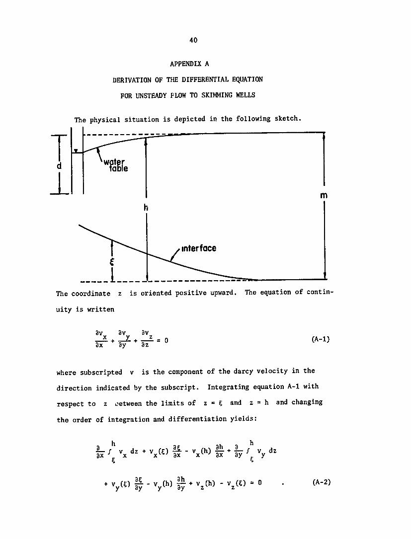
The physical situation is depicted in the following sketch

d

h

interface

-pound----------The coordinate z is oriented positive upward The equation of continshy

uity is written

avav av (A-1)

x By az

where subscripted v is the component of the darcy velocity in the

direction indicated by the subscript Integrating equation A-1 with

z = C and z = h and changingrespect to z oetween the limits of

the order of integration and differentiation yields

ha h ax v dz + v(C) 1 v ah + l- fVy dz

- V(h) - ayaa

ah + v=h 0 (A-2)+ V y()E--v(h)+ y y a+ Vzh v z

41

The vertical component of darcy velocity at the water table and at

the interface are given by

v (h)= (A-3)z dt

and

v (E)= 0 dt (A-4)Vz ( =euro dt

respectively Calculating the total derivative of h and E with

respect to time yields

dh 3h dx + ah + _ (A-S)

dt xdt aydt at

and d Dampadx + aE dL + a_amp (A-6)

dt x dt y dt at

The factors dxdt and dydt are the actual velocities components of

the interfaces Substituting equations A-5 and A-6 into equations A-3

and A-4 and expressing dxdt and dydt in terms of Darcy velocity

yields

h 8h h(A7 v (h) =vx(h) L- + vy(h) 2- +0 (A-7)

and

+ + v () = v (E) c vy (A-8)

Equations A-7 and A-8 can be substituted into equation A-2 to yield

fvh x dz + y- f h vy dz or0 (h - )(A-9)

42

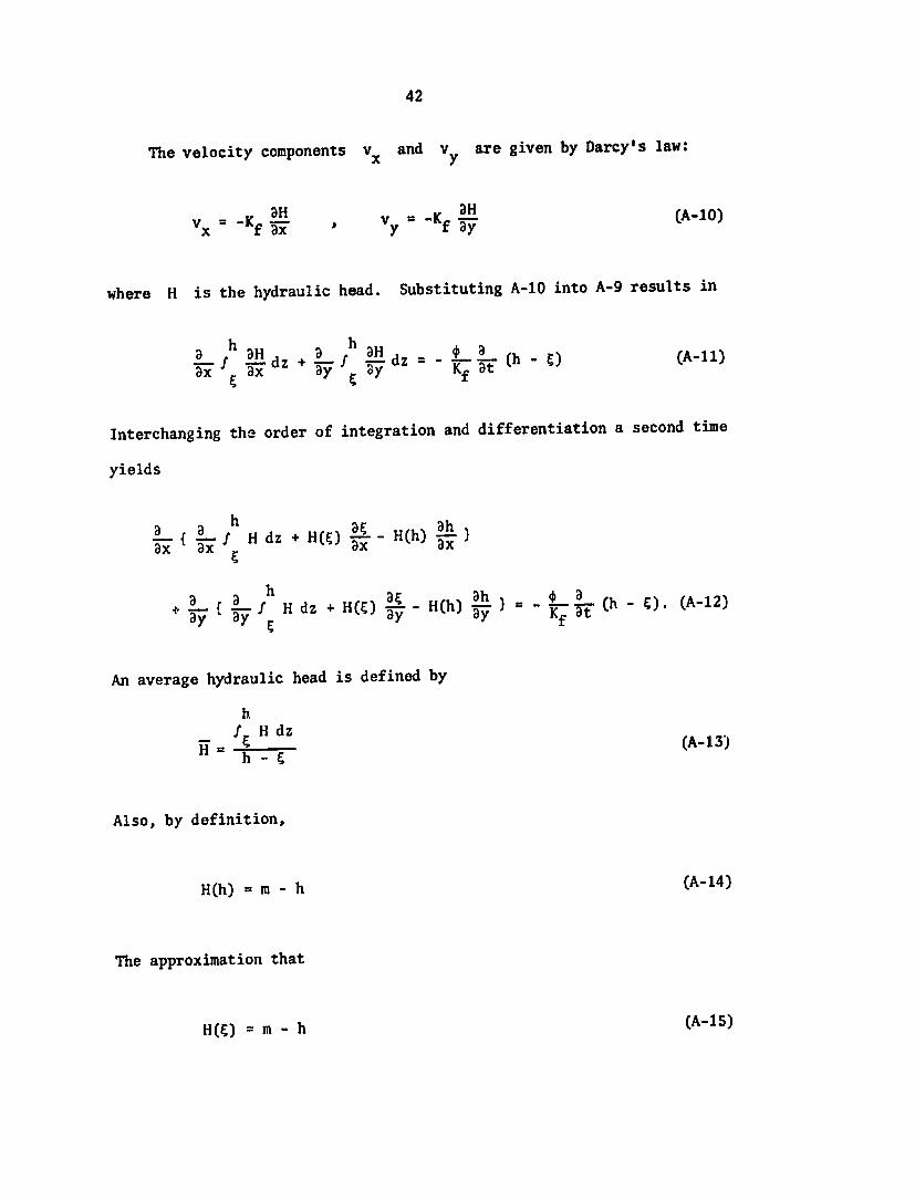
The velocity components vx and Vy are given by Darcys law

vx =-f ax v =-- -Kf By CA-10)=-Kf3H

where H is the hydraulic head Substituting A-10 into A-9 results in

fh 8H h a BHx dz + fh dz = - - B (h - ) (A-11)

Interchanging the order of integration and differentiation a second time

yields

- H dz + H( ) - H(h)1

a axEax ax

a 2 f Hd+H()a- H(h) =h a (h - E) (A-12)

An average hydraulic head is defined by

h fE H dz (A-13)

h -C

Also by definition

(A-14)H(h) = m - h

The approximation that

(A-is)H(E) = m - h

43

is also made Substitution of equations A-13 through A-15 into A-12

gives

- a (h- ) +[ h h)

K a (h - (A-16)

y is indicated by dots for where the equivalent term in the variable

convenience in notation

TIis equal to (m - h) and It is assumed that the average head

A-16 becomes

I + (h- ) (A-17)(h

h The Ghyben-Herzberg approximation is used to relate

the variables

and E by

(A-18)h = m -A

Yf

Substitution of A-18 into A-17 and considerable rearrangement eventually

yields

32 a2m m 2 a- 1 + AYlYf -a I + AYT~f

ay2ax2 Y

( Y+ - aKf - - (A-19)

Yf I+ Yf

44

Defining a new variable by

m +)2 (A-20)

allows equation A-19 to be written as

ax 2 2Dy Ay Kf at

Equation A-21 is non-linear because of the dependence of the coefficient

of at on Arbitrarily taking this coefficient to be constant

linearizes the equation and allows one to obtain solutions which are

useful for engineering purposes Therefore A-21 is rewritten as

2D2 9 _____Yf a_ (A-22) 2 2 Ay Kf T ataX ay

where T is an estimated weighted average of A large number of

solutions to equation A-22 for various initial and boundary conditions

are available in the literature

To complete the formulation an expression for the flux of fresh

water is required This is obtained from

h q= Kf f -dz (A-23)

Equation A-23 is a definition of an average fresh water flux in the

direction pound across a vertical plane Interchanging the order of

differentiation and integration yields

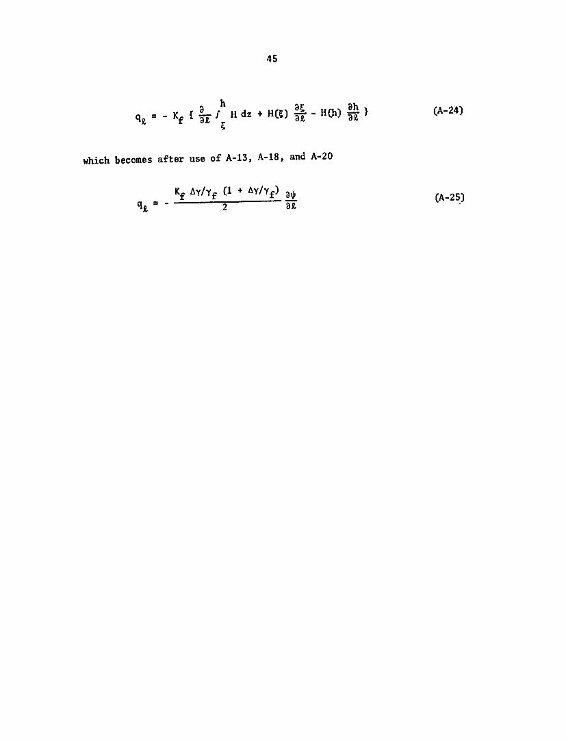
45

~n ah= h

q K -h Hdz + H(E) H~( h- (A-24)

which becomes after use of A-13 A-18 and A-20

Kf Ayf (1 + AyYf) (A-25) at)2

46

APPENDIX B

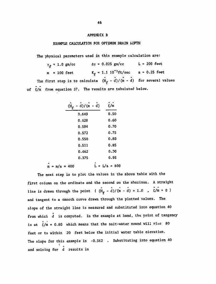
EXAMPLE CALCULATION FOR OPTIMUM DRAIN DEPTH

The physical parameters used in this example calculation are

Yf = 10 gmcc Ay = 0025 gmcc L = 200 feet

m = 100 feet Kf = 11 10 3ftsec a = 025 feet A A

The first step is to calculate (Hf - d)(m - d) for several values

of Zm from equation 37 The results are tabulated below

(Hf - d)(m - d) Em

0649 050

0628 060

0594 070

0572 075

0550 080

0511 085

0462 090

0375 095 AA

m =ma 400 L = La = 800

The next step is to plot the values in the above table with the

first column on the ordinate and the second on the abscissa A straight

line is drawn through the point (Hf - d)(m - d) = 10 Em = 0

and tangent to a smooth curve drawn through the plotted values The

slope of the straight line is measured and substituted into equation 40

from which d is computed In the example at hand the point of tangency

is at ^m 080 which means that the salt-water mound will ribe 80=

feet below the initial water table elevationfeet or to within 20

The slope for this example is -0562 Substituting into equation 40

and solving for d results in

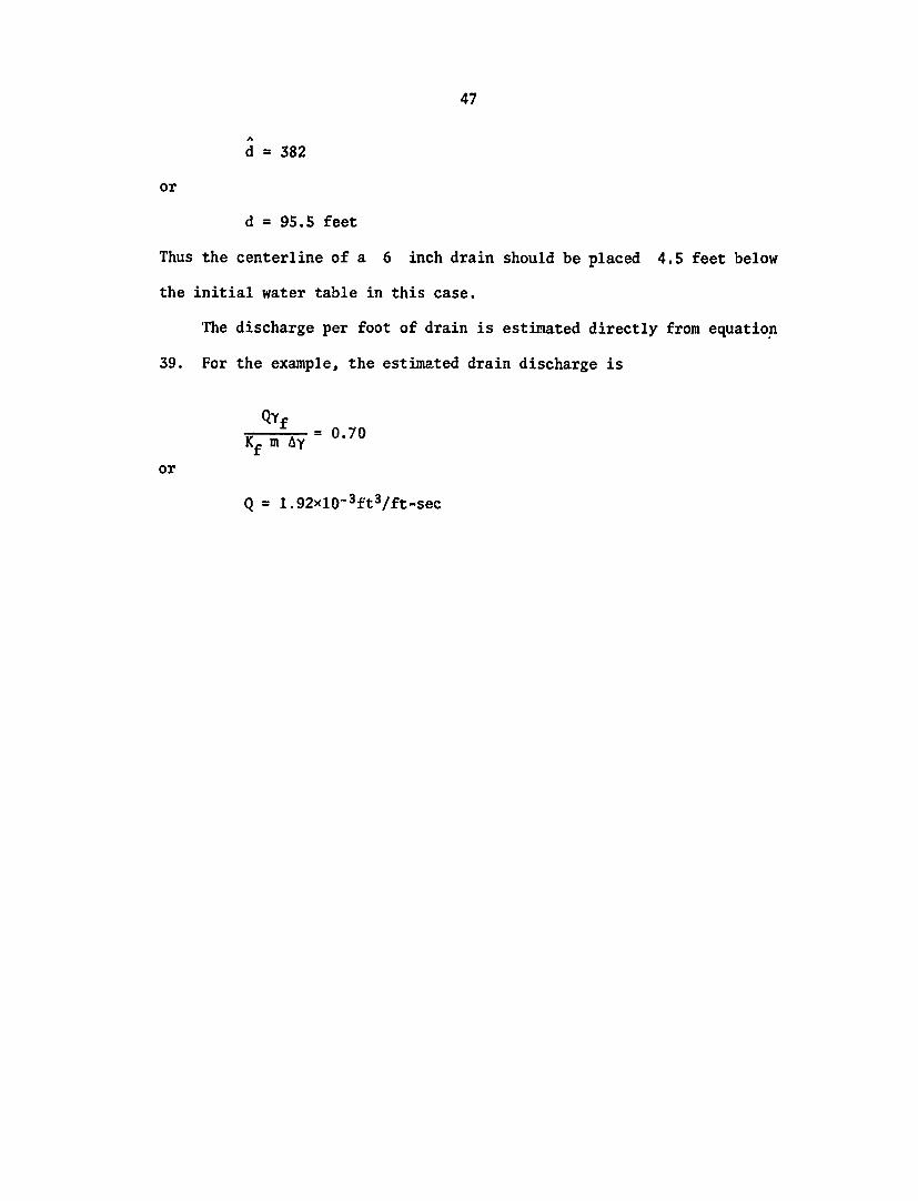
47

d = 382

or

d = 955 feet

Thus the centerline of a 6 inch drain should be placed 45 feet below

the initial water table in this case

The discharge per foot of drain is estimated directly from equation

39 For the example the estimated drain discharge is

QYf = 070

Kf m AT

or

Q = 192xlO-3ft3ft-sec

48

APPENDIX C

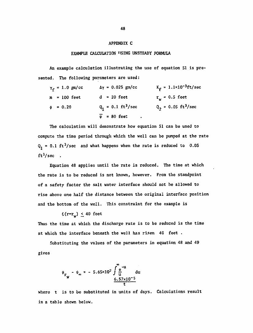
EXAMPLE CALCULATION IUSING UNSTEADY FORMULA

An example calculation illustrating the use of equation 51 is preshy

sented The following parameters are used

Yf = 10 gmcc Ay = 0025 gmcc Kf = 1lxlO3ftsec

m = 100 feet d = 20 feet rw = 05 feet

= 020 Q1 = 01 ft3sec Q2 = 005 ft3sec

T= 80 feet

The calculation will demonstrate how equation 51 can be used to

compute the time period through which the well can be pumped at the rate

Q1 = 01 ft3sec and what happens when the rate is reduced to 005

ft3sec

Equation 48 applies until the rate is reduced The time at which

the rate is to be reduced is not known however From the standpoint

of a safety factor the salt water interface should not be allowed to

rise above one half the distance between the original interface position

and the bottom of the well This constraint for the example is

E(r=rw) lt 40 feet

Thus the time at which the discharge rate is to be reduced is the time

at which the interface beneath the well has risen 40 feet

Substituting the values of the parameters in equation 48 and 49

gives

f-u - p = - 565x102Jf du

657x10-5

t

where t is to be substituted in units of days Calculations result

in a table shown below

49

u W(u) E(r=r) - ft t - days

- 5 3009051 657x10

-3 3289712 328x10

5 3624 164x10 1049

6 40010 657x10 1134

days the mound will have risen 40 feet beneath the well Thus at 10

For time larger than 10 days equation 51 is used

eu -u -2 I dudu + 282xi0 - 5=65x102 Je(r=rw) - 5

657x10657x10-5

tt

The results of calculations are shown below

t - days E(r=rW) - ft

3001

3282

3624

40010

36811

37014

38420

- -

CM UNS bullFM -COLORADO-

ri GWAER MANAGEMENTTEHNCA REPORTNO 20 -41Mshy


IN SALINE AQUIFERS


by

David B McWhorter





180



June 1972

AER71-72DBM27

______

-] w b + 7-bull - - 5 - ________ bull+ W U


David B McWhorter





1 6 Abieat











culations are given

AA


1T

l - (This 21-

j i C

J+ _____ _+4 +_ _ - T ___ ~L- 4

IL K ~ r3~ ~2





R Schmidt






U



G R

N Jones L Anderson

53 $300



180 $300





T Y Wu 98 $300


G N Jones 39 $300


G N Jones 77 $300


J W Hugh Barrett

106 $300









131 $300

TABLE OF CONTENTS

SUMMARY 1

INTRODUCTION

PROBLEM FORMULATION

3

4







Bear and Dagan 15

Wang 16

17McWhorter

Other Solutions

19





3SFUTURE WORK

36References

APPENDICES


SKIMMING WELLS 40



I

SUMMARY
















cussed











- Ishy

2


calculations given


3

INTRODUCTION



























4





















PROBLEM FORMULATION






5





















ac a Ic e

a xDi j ax - ()

in which


t = time - T


6


rank 2) - L2T


LT

















solving the problem







7



pkxi ag ) ] + S 2)

1 1 1

where


P = pressure - FL2



P = density - ML3


0 = porosity





liquid









8















inwhich



P = pressure - FL2







9


to obtain

V2Hf= 0 bull (5)










problem





H i y yf S- Eys (6)




10


s d i Yf 1 = s - Hf 7)



the interface



i Hi








with the horizontal





qf = qs P (10)

11





i yfqf

AyK sin (11)


fore the condition

i AyKf

qf Y (12)Yf







less than AyYf


Yf

A = - - Ah (13)





12


8H at = 0 S


or iTf

AE= - A- Hf (15)







flow


Muskat and Wyckoff











13





by

(16)Hf = Hf (rz)




Hf1 (17)= Hf (r )













14





situations exist



3) One root exists







cone height





charge






is

Bear and Dagan






is

L YfQ 1 (19)

d 21Td 2 Ay K [1+ r 2]1

in which




of interface - L





(20)CM lt f d



r27rfd2AyK [I+(j)21] (21)Qmax - f [1(=2](1

16



Wang










Mrerw m

where

s = drawdown - L


of well - L









17


QAykn rer 1w






heights

McWhorter











i

Yf qf (24) d Ay Kf





18


7shyre shy

z d h -interface

interface


--original




A = 2w (h-=)r (26)




(27)A=Ayfn +1L~) r

2S u m - (7- i1t 2A = y e p n r


19


I 1Qyenfpound nrrI





charge




remains stable

Other Solutions















20











table
















21

water table

drain radius =a


S-L






bull interface

-L


22



















mLXn

cosh--- 1



23


Yf i (32) Tf (m - Hf i )




- cosshycosh M











Hf - d Ay (35)

m-d = 1 - (------) fm




are defined

24

Hf = 1f a

d =da

m = ma (36)

L= La




m -d cosh nm^ 1

cosh ffLm - 1

Hfd d A (38)

A A

m -d m- f


Kf may cosh 7rm -1

cosh n Lm - I










25

AA A a AA




10

eq 3e

A A

Hf-d

A-a

eq 37

0 00







That is

m Ay (40)

m-dYf




26

placed









drain can be placed
















27















these equations












28
















equation

D2 = _ + YfS Z (42) t

aX2 By2 AyKf a

where

m )2 (43)


29


- Kf AYYf (1+ AYYf) 34 qX = 2 a (44)




















30













is given below






6) Legal


water levels







31











32 + 1 = a (45)

Dr2 r Dr at



2 = (-t) = m(l + AYpound))

(rO) = m(l + ATyTf)1 2 = o (47)



(48)2i0 W(u) 27 --(1+ -) Kf

Yf Yf

32

where

(9W(U) ffr2dId~ du

4t










02

I



ally in figure 6





33

C(r r)

A

0 time-t





time beyond t




(Q - Ql) W~t t (50)

21T - (1 + -) Kf

2

YfYf






n QI W(t) + E - Qi)W(t - ti-1 ) (51)

i=z

34


becomes


Q1 W(t) dT W(t - T) di (52)












n

T i (53)i=l1


the total

35

FUTURE WORK












steady flow




36

REFERENCES




1968



Amer Proc V 33 No 6 1969 pp 827-832




London











pp 2b-36




1967

37






No 2 pp 40=60



pp 221-244



V 16 Part 3pp 385-394






West Pakistan


May 1966



107




988

38




1971














Amer Proc V 34 1970 pp 412-417









No 4 pp 327-339

39



pp 875-882



Collips Colorado






pp 1290-1311



657



pp 5055-5063




40

APPENDIX A




d

h

interface


uity is written

avav av (A-1)

x By az






- V(h) - ayaa


41



v (h)= (A-3)z dt

and




dh 3h dx + ah + _ (A-S)

dt xdt aydt at


dt x dt y dt at




yields

h 8h h(A7 v (h) =vx(h) L- + vy(h) 2- +0 (A-7)

and

+ + v () = v (E) c vy (A-8)



42






yields

- H dz + H( ) - H(h)1

a axEax ax

a 2 f Hd+H()a- H(h) =h a (h - E) (A-12)


h fE H dz (A-13)

h -C

Also by definition

(A-14)H(h) = m - h


(A-is)H(E) = m - h

43


gives

- a (h- ) +[ h h)

K a (h - (A-16)




A-16 becomes

I + (h- ) (A-17)(h


the variables

and E by

(A-18)h = m -A

Yf


yields


ay2ax2 Y

( Y+ - aKf - - (A-19)

Yf I+ Yf

44


m +)2 (A-20)


ax 2 2Dy Ay Kf at















45

~n ah= h

q K -h Hdz + H(E) H~( h- (A-24)



46

APPENDIX B







(Hf - d)(m - d) Em

0649 050

0628 060

0594 070

0572 075

0550 080

0511 085

0462 090

0375 095 AA

m =ma 400 L = La = 800











47

d = 382

or

d = 955 feet





QYf = 070

Kf m AT

or


48

APPENDIX C






= 020 Q1 = 01 ft3sec Q2 = 005 ft3sec

T= 80 feet




ft3sec






E(r=rw) lt 40 feet




gives

f-u - p = - 565x102Jf du

657x10-5

t



49


- 5 3009051 657x10

-3 3289712 328x10

5 3624 164x10 1049

6 40010 657x10 1134




657x10657x10-5

tt



3001

3282

3624

40010

36811

37014

38420


IN SALINE AQUIFERS


by

David B McWhorter





180



June 1972

AER71-72DBM27

______

-] w b + 7-bull - - 5 - ________ bull+ W U


David B McWhorter





1 6 Abieat











culations are given

AA


1T

l - (This 21-

j i C

J+ _____ _+4 +_ _ - T ___ ~L- 4

IL K ~ r3~ ~2





R Schmidt






U



G R

N Jones L Anderson

53 $300



180 $300





T Y Wu 98 $300


G N Jones 39 $300


G N Jones 77 $300


J W Hugh Barrett

106 $300









131 $300

TABLE OF CONTENTS

SUMMARY 1

INTRODUCTION

PROBLEM FORMULATION

3

4







Bear and Dagan 15

Wang 16

17McWhorter

Other Solutions

19





3SFUTURE WORK

36References

APPENDICES


SKIMMING WELLS 40



I

SUMMARY
















cussed











- Ishy

2


calculations given


3

INTRODUCTION



























4





















PROBLEM FORMULATION






5





















ac a Ic e

a xDi j ax - ()

in which


t = time - T


6


rank 2) - L2T


LT

















solving the problem







7



pkxi ag ) ] + S 2)

1 1 1

where


P = pressure - FL2



P = density - ML3


0 = porosity





liquid









8















inwhich



P = pressure - FL2







9


to obtain

V2Hf= 0 bull (5)










problem





H i y yf S- Eys (6)




10


s d i Yf 1 = s - Hf 7)



the interface



i Hi








with the horizontal





qf = qs P (10)

11





i yfqf

AyK sin (11)


fore the condition

i AyKf

qf Y (12)Yf







less than AyYf


Yf

A = - - Ah (13)





12


8H at = 0 S


or iTf

AE= - A- Hf (15)







flow


Muskat and Wyckoff











13





by

(16)Hf = Hf (rz)




Hf1 (17)= Hf (r )













14





situations exist



3) One root exists







cone height





charge






is

Bear and Dagan






is

L YfQ 1 (19)

d 21Td 2 Ay K [1+ r 2]1

in which




of interface - L





(20)CM lt f d



r27rfd2AyK [I+(j)21] (21)Qmax - f [1(=2](1

16



Wang










Mrerw m

where

s = drawdown - L


of well - L









17


QAykn rer 1w






heights

McWhorter











i

Yf qf (24) d Ay Kf





18


7shyre shy

z d h -interface

interface


--original




A = 2w (h-=)r (26)




(27)A=Ayfn +1L~) r

2S u m - (7- i1t 2A = y e p n r


19


I 1Qyenfpound nrrI





charge




remains stable

Other Solutions















20











table
















21

water table

drain radius =a


S-L






bull interface

-L


22



















mLXn

cosh--- 1



23


Yf i (32) Tf (m - Hf i )




- cosshycosh M











Hf - d Ay (35)

m-d = 1 - (------) fm




are defined

24

Hf = 1f a

d =da

m = ma (36)

L= La




m -d cosh nm^ 1

cosh ffLm - 1

Hfd d A (38)

A A

m -d m- f


Kf may cosh 7rm -1

cosh n Lm - I










25

AA A a AA




10

eq 3e

A A

Hf-d

A-a

eq 37

0 00







That is

m Ay (40)

m-dYf




26

placed









drain can be placed
















27















these equations












28
















equation

D2 = _ + YfS Z (42) t

aX2 By2 AyKf a

where

m )2 (43)


29


- Kf AYYf (1+ AYYf) 34 qX = 2 a (44)




















30













is given below






6) Legal


water levels







31











32 + 1 = a (45)

Dr2 r Dr at



2 = (-t) = m(l + AYpound))

(rO) = m(l + ATyTf)1 2 = o (47)



(48)2i0 W(u) 27 --(1+ -) Kf

Yf Yf

32

where

(9W(U) ffr2dId~ du

4t










02

I



ally in figure 6





33

C(r r)

A

0 time-t





time beyond t




(Q - Ql) W~t t (50)

21T - (1 + -) Kf

2

YfYf






n QI W(t) + E - Qi)W(t - ti-1 ) (51)

i=z

34


becomes


Q1 W(t) dT W(t - T) di (52)












n

T i (53)i=l1


the total

35

FUTURE WORK












steady flow




36

REFERENCES




1968



Amer Proc V 33 No 6 1969 pp 827-832




London











pp 2b-36




1967

37






No 2 pp 40=60



pp 221-244



V 16 Part 3pp 385-394






West Pakistan


May 1966



107




988

38




1971














Amer Proc V 34 1970 pp 412-417









No 4 pp 327-339

39



pp 875-882



Collips Colorado






pp 1290-1311



657



pp 5055-5063




40

APPENDIX A




d

h

interface


uity is written

avav av (A-1)

x By az






- V(h) - ayaa


41



v (h)= (A-3)z dt

and




dh 3h dx + ah + _ (A-S)

dt xdt aydt at


dt x dt y dt at




yields

h 8h h(A7 v (h) =vx(h) L- + vy(h) 2- +0 (A-7)

and

+ + v () = v (E) c vy (A-8)



42






yields

- H dz + H( ) - H(h)1

a axEax ax

a 2 f Hd+H()a- H(h) =h a (h - E) (A-12)


h fE H dz (A-13)

h -C

Also by definition

(A-14)H(h) = m - h


(A-is)H(E) = m - h

43


gives

- a (h- ) +[ h h)

K a (h - (A-16)




A-16 becomes

I + (h- ) (A-17)(h


the variables

and E by

(A-18)h = m -A

Yf


yields


ay2ax2 Y

( Y+ - aKf - - (A-19)

Yf I+ Yf

44


m +)2 (A-20)


ax 2 2Dy Ay Kf at















45

~n ah= h

q K -h Hdz + H(E) H~( h- (A-24)



46

APPENDIX B







(Hf - d)(m - d) Em

0649 050

0628 060

0594 070

0572 075

0550 080

0511 085

0462 090

0375 095 AA

m =ma 400 L = La = 800











47

d = 382

or

d = 955 feet





QYf = 070

Kf m AT

or


48

APPENDIX C






= 020 Q1 = 01 ft3sec Q2 = 005 ft3sec

T= 80 feet




ft3sec






E(r=rw) lt 40 feet




gives

f-u - p = - 565x102Jf du

657x10-5

t



49


- 5 3009051 657x10

-3 3289712 328x10

5 3624 164x10 1049

6 40010 657x10 1134




657x10657x10-5

tt



3001

3282

3624

40010

36811

37014

38420

______

-] w b + 7-bull - - 5 - ________ bull+ W U


David B McWhorter





1 6 Abieat











culations are given

AA


1T

l - (This 21-

j i C

J+ _____ _+4 +_ _ - T ___ ~L- 4

IL K ~ r3~ ~2





R Schmidt






U



G R

N Jones L Anderson

53 $300



180 $300





T Y Wu 98 $300


G N Jones 39 $300


G N Jones 77 $300


J W Hugh Barrett

106 $300









131 $300

TABLE OF CONTENTS

SUMMARY 1

INTRODUCTION

PROBLEM FORMULATION

3

4







Bear and Dagan 15

Wang 16

17McWhorter

Other Solutions

19





3SFUTURE WORK

36References

APPENDICES


SKIMMING WELLS 40



I

SUMMARY
















cussed











- Ishy

2


calculations given


3

INTRODUCTION



























4





















PROBLEM FORMULATION






5





















ac a Ic e

a xDi j ax - ()

in which


t = time - T


6


rank 2) - L2T


LT

















solving the problem







7



pkxi ag ) ] + S 2)

1 1 1

where


P = pressure - FL2



P = density - ML3


0 = porosity





liquid









8















inwhich



P = pressure - FL2







9


to obtain

V2Hf= 0 bull (5)










problem





H i y yf S- Eys (6)




10


s d i Yf 1 = s - Hf 7)



the interface



i Hi








with the horizontal





qf = qs P (10)

11





i yfqf

AyK sin (11)


fore the condition

i AyKf

qf Y (12)Yf







less than AyYf


Yf

A = - - Ah (13)





12


8H at = 0 S


or iTf

AE= - A- Hf (15)







flow


Muskat and Wyckoff











13





by

(16)Hf = Hf (rz)




Hf1 (17)= Hf (r )













14





situations exist



3) One root exists







cone height





charge






is

Bear and Dagan






is

L YfQ 1 (19)

d 21Td 2 Ay K [1+ r 2]1

in which




of interface - L





(20)CM lt f d



r27rfd2AyK [I+(j)21] (21)Qmax - f [1(=2](1

16



Wang










Mrerw m

where

s = drawdown - L


of well - L









17


QAykn rer 1w






heights

McWhorter











i

Yf qf (24) d Ay Kf





18


7shyre shy

z d h -interface

interface


--original




A = 2w (h-=)r (26)




(27)A=Ayfn +1L~) r

2S u m - (7- i1t 2A = y e p n r


19


I 1Qyenfpound nrrI





charge




remains stable

Other Solutions















20











table
















21

water table

drain radius =a


S-L






bull interface

-L


22



















mLXn

cosh--- 1



23


Yf i (32) Tf (m - Hf i )




- cosshycosh M











Hf - d Ay (35)

m-d = 1 - (------) fm




are defined

24

Hf = 1f a

d =da

m = ma (36)

L= La




m -d cosh nm^ 1

cosh ffLm - 1

Hfd d A (38)

A A

m -d m- f


Kf may cosh 7rm -1

cosh n Lm - I










25

AA A a AA




10

eq 3e

A A

Hf-d

A-a

eq 37

0 00







That is

m Ay (40)

m-dYf




26

placed









drain can be placed
















27















these equations












28
















equation

D2 = _ + YfS Z (42) t

aX2 By2 AyKf a

where

m )2 (43)


29


- Kf AYYf (1+ AYYf) 34 qX = 2 a (44)




















30













is given below






6) Legal


water levels







31











32 + 1 = a (45)

Dr2 r Dr at



2 = (-t) = m(l + AYpound))

(rO) = m(l + ATyTf)1 2 = o (47)



(48)2i0 W(u) 27 --(1+ -) Kf

Yf Yf

32

where

(9W(U) ffr2dId~ du

4t










02

I



ally in figure 6





33

C(r r)

A

0 time-t





time beyond t




(Q - Ql) W~t t (50)

21T - (1 + -) Kf

2

YfYf






n QI W(t) + E - Qi)W(t - ti-1 ) (51)

i=z

34


becomes


Q1 W(t) dT W(t - T) di (52)












n

T i (53)i=l1


the total

35

FUTURE WORK












steady flow




36

REFERENCES




1968



Amer Proc V 33 No 6 1969 pp 827-832




London











pp 2b-36




1967

37






No 2 pp 40=60



pp 221-244



V 16 Part 3pp 385-394






West Pakistan


May 1966



107




988

38




1971














Amer Proc V 34 1970 pp 412-417









No 4 pp 327-339

39



pp 875-882



Collips Colorado






pp 1290-1311



657



pp 5055-5063




40

APPENDIX A




d

h

interface


uity is written

avav av (A-1)

x By az






- V(h) - ayaa


41



v (h)= (A-3)z dt

and




dh 3h dx + ah + _ (A-S)

dt xdt aydt at


dt x dt y dt at




yields

h 8h h(A7 v (h) =vx(h) L- + vy(h) 2- +0 (A-7)

and

+ + v () = v (E) c vy (A-8)



42






yields

- H dz + H( ) - H(h)1

a axEax ax

a 2 f Hd+H()a- H(h) =h a (h - E) (A-12)


h fE H dz (A-13)

h -C

Also by definition

(A-14)H(h) = m - h


(A-is)H(E) = m - h

43


gives

- a (h- ) +[ h h)

K a (h - (A-16)




A-16 becomes

I + (h- ) (A-17)(h


the variables

and E by

(A-18)h = m -A

Yf


yields


ay2ax2 Y

( Y+ - aKf - - (A-19)

Yf I+ Yf

44


m +)2 (A-20)


ax 2 2Dy Ay Kf at















45

~n ah= h

q K -h Hdz + H(E) H~( h- (A-24)



46

APPENDIX B







(Hf - d)(m - d) Em

0649 050

0628 060

0594 070

0572 075

0550 080

0511 085

0462 090

0375 095 AA

m =ma 400 L = La = 800











47

d = 382

or

d = 955 feet





QYf = 070

Kf m AT

or


48

APPENDIX C






= 020 Q1 = 01 ft3sec Q2 = 005 ft3sec

T= 80 feet




ft3sec






E(r=rw) lt 40 feet




gives

f-u - p = - 565x102Jf du

657x10-5

t



49


- 5 3009051 657x10

-3 3289712 328x10

5 3624 164x10 1049

6 40010 657x10 1134




657x10657x10-5

tt



3001

3282

3624

40010

36811

37014

38420





R Schmidt






U



G R

N Jones L Anderson

53 $300



180 $300





T Y Wu 98 $300


G N Jones 39 $300


G N Jones 77 $300


J W Hugh Barrett

106 $300









131 $300

TABLE OF CONTENTS

SUMMARY 1

INTRODUCTION

PROBLEM FORMULATION

3

4







Bear and Dagan 15

Wang 16

17McWhorter

Other Solutions

19





3SFUTURE WORK

36References

APPENDICES


SKIMMING WELLS 40



I

SUMMARY
















cussed











- Ishy

2


calculations given


3

INTRODUCTION



























4





















PROBLEM FORMULATION






5





















ac a Ic e

a xDi j ax - ()

in which


t = time - T


6


rank 2) - L2T


LT

















solving the problem







7



pkxi ag ) ] + S 2)

1 1 1

where


P = pressure - FL2



P = density - ML3


0 = porosity





liquid









8















inwhich



P = pressure - FL2







9


to obtain

V2Hf= 0 bull (5)










problem





H i y yf S- Eys (6)




10


s d i Yf 1 = s - Hf 7)



the interface



i Hi








with the horizontal





qf = qs P (10)

11





i yfqf

AyK sin (11)


fore the condition

i AyKf

qf Y (12)Yf







less than AyYf


Yf

A = - - Ah (13)





12


8H at = 0 S


or iTf

AE= - A- Hf (15)







flow


Muskat and Wyckoff











13





by

(16)Hf = Hf (rz)




Hf1 (17)= Hf (r )













14





situations exist



3) One root exists







cone height





charge






is

Bear and Dagan






is

L YfQ 1 (19)

d 21Td 2 Ay K [1+ r 2]1

in which




of interface - L





(20)CM lt f d



r27rfd2AyK [I+(j)21] (21)Qmax - f [1(=2](1

16



Wang










Mrerw m

where

s = drawdown - L


of well - L









17


QAykn rer 1w






heights

McWhorter











i

Yf qf (24) d Ay Kf





18


7shyre shy

z d h -interface

interface


--original




A = 2w (h-=)r (26)




(27)A=Ayfn +1L~) r

2S u m - (7- i1t 2A = y e p n r


19


I 1Qyenfpound nrrI





charge




remains stable

Other Solutions















20











table
















21

water table

drain radius =a


S-L






bull interface

-L


22



















mLXn

cosh--- 1



23


Yf i (32) Tf (m - Hf i )




- cosshycosh M











Hf - d Ay (35)

m-d = 1 - (------) fm




are defined

24

Hf = 1f a

d =da

m = ma (36)

L= La




m -d cosh nm^ 1

cosh ffLm - 1

Hfd d A (38)

A A

m -d m- f


Kf may cosh 7rm -1

cosh n Lm - I










25

AA A a AA




10

eq 3e

A A

Hf-d

A-a

eq 37

0 00







That is

m Ay (40)

m-dYf




26

placed









drain can be placed
















27















these equations












28
















equation

D2 = _ + YfS Z (42) t

aX2 By2 AyKf a

where

m )2 (43)


29


- Kf AYYf (1+ AYYf) 34 qX = 2 a (44)




















30













is given below






6) Legal


water levels







31











32 + 1 = a (45)

Dr2 r Dr at



2 = (-t) = m(l + AYpound))

(rO) = m(l + ATyTf)1 2 = o (47)



(48)2i0 W(u) 27 --(1+ -) Kf

Yf Yf

32

where

(9W(U) ffr2dId~ du

4t










02

I



ally in figure 6





33

C(r r)

A

0 time-t





time beyond t




(Q - Ql) W~t t (50)

21T - (1 + -) Kf

2

YfYf






n QI W(t) + E - Qi)W(t - ti-1 ) (51)

i=z

34


becomes


Q1 W(t) dT W(t - T) di (52)












n

T i (53)i=l1


the total

35

FUTURE WORK












steady flow




36

REFERENCES




1968



Amer Proc V 33 No 6 1969 pp 827-832




London











pp 2b-36




1967

37






No 2 pp 40=60



pp 221-244



V 16 Part 3pp 385-394






West Pakistan


May 1966



107




988

38




1971














Amer Proc V 34 1970 pp 412-417









No 4 pp 327-339

39



pp 875-882



Collips Colorado






pp 1290-1311



657



pp 5055-5063




40

APPENDIX A




d

h

interface


uity is written

avav av (A-1)

x By az






- V(h) - ayaa


41



v (h)= (A-3)z dt

and




dh 3h dx + ah + _ (A-S)

dt xdt aydt at


dt x dt y dt at




yields

h 8h h(A7 v (h) =vx(h) L- + vy(h) 2- +0 (A-7)

and

+ + v () = v (E) c vy (A-8)



42






yields

- H dz + H( ) - H(h)1

a axEax ax

a 2 f Hd+H()a- H(h) =h a (h - E) (A-12)


h fE H dz (A-13)

h -C

Also by definition

(A-14)H(h) = m - h


(A-is)H(E) = m - h

43


gives

- a (h- ) +[ h h)

K a (h - (A-16)




A-16 becomes

I + (h- ) (A-17)(h


the variables

and E by

(A-18)h = m -A

Yf


yields


ay2ax2 Y

( Y+ - aKf - - (A-19)

Yf I+ Yf

44


m +)2 (A-20)


ax 2 2Dy Ay Kf at















45

~n ah= h

q K -h Hdz + H(E) H~( h- (A-24)



46

APPENDIX B







(Hf - d)(m - d) Em

0649 050

0628 060

0594 070

0572 075

0550 080

0511 085

0462 090

0375 095 AA

m =ma 400 L = La = 800











47

d = 382

or

d = 955 feet





QYf = 070

Kf m AT

or


48

APPENDIX C






= 020 Q1 = 01 ft3sec Q2 = 005 ft3sec

T= 80 feet




ft3sec






E(r=rw) lt 40 feet




gives

f-u - p = - 565x102Jf du

657x10-5

t



49


- 5 3009051 657x10

-3 3289712 328x10

5 3624 164x10 1049

6 40010 657x10 1134




657x10657x10-5

tt



3001

3282

3624

40010

36811

37014

38420



G R

N Jones L Anderson

53 $300



180 $300





T Y Wu 98 $300


G N Jones 39 $300


G N Jones 77 $300


J W Hugh Barrett

106 $300









131 $300

TABLE OF CONTENTS

SUMMARY 1

INTRODUCTION

PROBLEM FORMULATION

3

4







Bear and Dagan 15

Wang 16

17McWhorter

Other Solutions

19





3SFUTURE WORK

36References

APPENDICES


SKIMMING WELLS 40



I

SUMMARY
















cussed











- Ishy

2


calculations given


3

INTRODUCTION



























4





















PROBLEM FORMULATION






5





















ac a Ic e

a xDi j ax - ()

in which


t = time - T


6


rank 2) - L2T


LT

















solving the problem







7



pkxi ag ) ] + S 2)

1 1 1

where


P = pressure - FL2



P = density - ML3


0 = porosity





liquid









8















inwhich



P = pressure - FL2







9


to obtain

V2Hf= 0 bull (5)










problem





H i y yf S- Eys (6)




10


s d i Yf 1 = s - Hf 7)



the interface



i Hi








with the horizontal





qf = qs P (10)

11





i yfqf

AyK sin (11)


fore the condition

i AyKf

qf Y (12)Yf







less than AyYf


Yf

A = - - Ah (13)





12


8H at = 0 S


or iTf

AE= - A- Hf (15)







flow


Muskat and Wyckoff











13





by

(16)Hf = Hf (rz)




Hf1 (17)= Hf (r )













14





situations exist



3) One root exists







cone height





charge






is

Bear and Dagan






is

L YfQ 1 (19)

d 21Td 2 Ay K [1+ r 2]1

in which




of interface - L





(20)CM lt f d



r27rfd2AyK [I+(j)21] (21)Qmax - f [1(=2](1

16



Wang










Mrerw m

where

s = drawdown - L


of well - L









17


QAykn rer 1w






heights

McWhorter











i

Yf qf (24) d Ay Kf





18


7shyre shy

z d h -interface

interface


--original




A = 2w (h-=)r (26)




(27)A=Ayfn +1L~) r

2S u m - (7- i1t 2A = y e p n r


19


I 1Qyenfpound nrrI





charge




remains stable

Other Solutions















20











table
















21

water table

drain radius =a


S-L






bull interface

-L


22



















mLXn

cosh--- 1



23


Yf i (32) Tf (m - Hf i )




- cosshycosh M











Hf - d Ay (35)

m-d = 1 - (------) fm




are defined

24

Hf = 1f a

d =da

m = ma (36)

L= La




m -d cosh nm^ 1

cosh ffLm - 1

Hfd d A (38)

A A

m -d m- f


Kf may cosh 7rm -1

cosh n Lm - I










25

AA A a AA




10

eq 3e

A A

Hf-d

A-a

eq 37

0 00







That is

m Ay (40)

m-dYf




26

placed









drain can be placed
















27















these equations












28
















equation

D2 = _ + YfS Z (42) t

aX2 By2 AyKf a

where

m )2 (43)


29


- Kf AYYf (1+ AYYf) 34 qX = 2 a (44)




















30













is given below






6) Legal


water levels







31











32 + 1 = a (45)

Dr2 r Dr at



2 = (-t) = m(l + AYpound))

(rO) = m(l + ATyTf)1 2 = o (47)



(48)2i0 W(u) 27 --(1+ -) Kf

Yf Yf

32

where

(9W(U) ffr2dId~ du

4t










02

I



ally in figure 6





33

C(r r)

A

0 time-t





time beyond t




(Q - Ql) W~t t (50)

21T - (1 + -) Kf

2

YfYf






n QI W(t) + E - Qi)W(t - ti-1 ) (51)

i=z

34


becomes


Q1 W(t) dT W(t - T) di (52)












n

T i (53)i=l1


the total

35

FUTURE WORK












steady flow




36

REFERENCES




1968



Amer Proc V 33 No 6 1969 pp 827-832




London











pp 2b-36




1967

37






No 2 pp 40=60



pp 221-244



V 16 Part 3pp 385-394






West Pakistan


May 1966



107




988

38




1971














Amer Proc V 34 1970 pp 412-417









No 4 pp 327-339

39



pp 875-882



Collips Colorado






pp 1290-1311



657



pp 5055-5063




40

APPENDIX A




d

h

interface


uity is written

avav av (A-1)

x By az






- V(h) - ayaa


41



v (h)= (A-3)z dt

and




dh 3h dx + ah + _ (A-S)

dt xdt aydt at


dt x dt y dt at




yields

h 8h h(A7 v (h) =vx(h) L- + vy(h) 2- +0 (A-7)

and

+ + v () = v (E) c vy (A-8)



42






yields

- H dz + H( ) - H(h)1

a axEax ax

a 2 f Hd+H()a- H(h) =h a (h - E) (A-12)


h fE H dz (A-13)

h -C

Also by definition

(A-14)H(h) = m - h


(A-is)H(E) = m - h

43


gives

- a (h- ) +[ h h)

K a (h - (A-16)




A-16 becomes

I + (h- ) (A-17)(h


the variables

and E by

(A-18)h = m -A

Yf


yields


ay2ax2 Y

( Y+ - aKf - - (A-19)

Yf I+ Yf

44


m +)2 (A-20)


ax 2 2Dy Ay Kf at















45

~n ah= h

q K -h Hdz + H(E) H~( h- (A-24)



46

APPENDIX B







(Hf - d)(m - d) Em

0649 050

0628 060

0594 070

0572 075

0550 080

0511 085

0462 090

0375 095 AA

m =ma 400 L = La = 800











47

d = 382

or

d = 955 feet





QYf = 070

Kf m AT

or


48

APPENDIX C






= 020 Q1 = 01 ft3sec Q2 = 005 ft3sec

T= 80 feet




ft3sec






E(r=rw) lt 40 feet




gives

f-u - p = - 565x102Jf du

657x10-5

t



49


- 5 3009051 657x10

-3 3289712 328x10

5 3624 164x10 1049

6 40010 657x10 1134




657x10657x10-5

tt



3001

3282

3624

40010

36811

37014

38420

TABLE OF CONTENTS

SUMMARY 1

INTRODUCTION

PROBLEM FORMULATION

3

4







Bear and Dagan 15

Wang 16

17McWhorter

Other Solutions

19





3SFUTURE WORK

36References

APPENDICES


SKIMMING WELLS 40



I

SUMMARY
















cussed











- Ishy

2


calculations given


3

INTRODUCTION



























4





















PROBLEM FORMULATION






5





















ac a Ic e

a xDi j ax - ()

in which


t = time - T


6


rank 2) - L2T


LT

















solving the problem







7



pkxi ag ) ] + S 2)

1 1 1

where


P = pressure - FL2



P = density - ML3


0 = porosity





liquid









8















inwhich



P = pressure - FL2







9


to obtain

V2Hf= 0 bull (5)










problem





H i y yf S- Eys (6)




10


s d i Yf 1 = s - Hf 7)



the interface



i Hi








with the horizontal





qf = qs P (10)

11





i yfqf

AyK sin (11)


fore the condition

i AyKf

qf Y (12)Yf







less than AyYf


Yf

A = - - Ah (13)





12


8H at = 0 S


or iTf

AE= - A- Hf (15)







flow


Muskat and Wyckoff











13





by

(16)Hf = Hf (rz)




Hf1 (17)= Hf (r )













14





situations exist



3) One root exists







cone height





charge






is

Bear and Dagan






is

L YfQ 1 (19)

d 21Td 2 Ay K [1+ r 2]1

in which




of interface - L





(20)CM lt f d



r27rfd2AyK [I+(j)21] (21)Qmax - f [1(=2](1

16



Wang










Mrerw m

where

s = drawdown - L


of well - L









17


QAykn rer 1w






heights

McWhorter











i

Yf qf (24) d Ay Kf





18


7shyre shy

z d h -interface

interface


--original




A = 2w (h-=)r (26)




(27)A=Ayfn +1L~) r

2S u m - (7- i1t 2A = y e p n r


19


I 1Qyenfpound nrrI





charge




remains stable

Other Solutions















20











table
















21

water table

drain radius =a


S-L






bull interface

-L


22



















mLXn

cosh--- 1



23


Yf i (32) Tf (m - Hf i )




- cosshycosh M











Hf - d Ay (35)

m-d = 1 - (------) fm




are defined

24

Hf = 1f a

d =da

m = ma (36)

L= La




m -d cosh nm^ 1

cosh ffLm - 1

Hfd d A (38)

A A

m -d m- f


Kf may cosh 7rm -1

cosh n Lm - I










25

AA A a AA




10

eq 3e

A A

Hf-d

A-a

eq 37

0 00







That is

m Ay (40)

m-dYf




26

placed









drain can be placed
















27















these equations












28
















equation

D2 = _ + YfS Z (42) t

aX2 By2 AyKf a

where

m )2 (43)


29


- Kf AYYf (1+ AYYf) 34 qX = 2 a (44)




















30













is given below






6) Legal


water levels







31











32 + 1 = a (45)

Dr2 r Dr at



2 = (-t) = m(l + AYpound))

(rO) = m(l + ATyTf)1 2 = o (47)



(48)2i0 W(u) 27 --(1+ -) Kf

Yf Yf

32

where

(9W(U) ffr2dId~ du

4t










02

I



ally in figure 6





33

C(r r)

A

0 time-t





time beyond t




(Q - Ql) W~t t (50)

21T - (1 + -) Kf

2

YfYf






n QI W(t) + E - Qi)W(t - ti-1 ) (51)

i=z

34


becomes


Q1 W(t) dT W(t - T) di (52)












n

T i (53)i=l1


the total

35

FUTURE WORK












steady flow




36

REFERENCES




1968



Amer Proc V 33 No 6 1969 pp 827-832




London











pp 2b-36




1967

37






No 2 pp 40=60



pp 221-244



V 16 Part 3pp 385-394






West Pakistan


May 1966



107




988

38




1971














Amer Proc V 34 1970 pp 412-417









No 4 pp 327-339

39



pp 875-882



Collips Colorado






pp 1290-1311



657



pp 5055-5063




40

APPENDIX A




d

h

interface


uity is written

avav av (A-1)

x By az






- V(h) - ayaa


41



v (h)= (A-3)z dt

and




dh 3h dx + ah + _ (A-S)

dt xdt aydt at


dt x dt y dt at




yields

h 8h h(A7 v (h) =vx(h) L- + vy(h) 2- +0 (A-7)

and

+ + v () = v (E) c vy (A-8)



42






yields

- H dz + H( ) - H(h)1

a axEax ax

a 2 f Hd+H()a- H(h) =h a (h - E) (A-12)


h fE H dz (A-13)

h -C

Also by definition

(A-14)H(h) = m - h


(A-is)H(E) = m - h

43


gives

- a (h- ) +[ h h)

K a (h - (A-16)




A-16 becomes

I + (h- ) (A-17)(h


the variables

and E by

(A-18)h = m -A

Yf


yields


ay2ax2 Y

( Y+ - aKf - - (A-19)

Yf I+ Yf

44


m +)2 (A-20)


ax 2 2Dy Ay Kf at















45

~n ah= h

q K -h Hdz + H(E) H~( h- (A-24)



46

APPENDIX B







(Hf - d)(m - d) Em

0649 050

0628 060

0594 070

0572 075

0550 080

0511 085

0462 090

0375 095 AA

m =ma 400 L = La = 800











47

d = 382

or

d = 955 feet





QYf = 070

Kf m AT

or


48

APPENDIX C






= 020 Q1 = 01 ft3sec Q2 = 005 ft3sec

T= 80 feet




ft3sec






E(r=rw) lt 40 feet




gives

f-u - p = - 565x102Jf du

657x10-5

t



49


- 5 3009051 657x10

-3 3289712 328x10

5 3624 164x10 1049

6 40010 657x10 1134




657x10657x10-5

tt



3001

3282

3624

40010

36811

37014

38420

SUMMARY
















cussed











- Ishy

2


calculations given


3

INTRODUCTION



























4





















PROBLEM FORMULATION






5





















ac a Ic e

a xDi j ax - ()

in which


t = time - T


6


rank 2) - L2T


LT

















solving the problem







7



pkxi ag ) ] + S 2)

1 1 1

where


P = pressure - FL2



P = density - ML3


0 = porosity





liquid









8















inwhich



P = pressure - FL2







9


to obtain

V2Hf= 0 bull (5)










problem





H i y yf S- Eys (6)




10


s d i Yf 1 = s - Hf 7)



the interface



i Hi








with the horizontal





qf = qs P (10)

11





i yfqf

AyK sin (11)


fore the condition

i AyKf

qf Y (12)Yf







less than AyYf


Yf

A = - - Ah (13)





12


8H at = 0 S


or iTf

AE= - A- Hf (15)







flow


Muskat and Wyckoff











13





by

(16)Hf = Hf (rz)




Hf1 (17)= Hf (r )













14





situations exist



3) One root exists







cone height





charge






is

Bear and Dagan






is

L YfQ 1 (19)

d 21Td 2 Ay K [1+ r 2]1

in which




of interface - L





(20)CM lt f d



r27rfd2AyK [I+(j)21] (21)Qmax - f [1(=2](1

16



Wang










Mrerw m

where

s = drawdown - L


of well - L









17


QAykn rer 1w






heights

McWhorter











i

Yf qf (24) d Ay Kf





18


7shyre shy

z d h -interface

interface


--original




A = 2w (h-=)r (26)




(27)A=Ayfn +1L~) r

2S u m - (7- i1t 2A = y e p n r


19


I 1Qyenfpound nrrI





charge




remains stable

Other Solutions















20











table
















21

water table

drain radius =a


S-L






bull interface

-L


22



















mLXn

cosh--- 1



23


Yf i (32) Tf (m - Hf i )




- cosshycosh M











Hf - d Ay (35)

m-d = 1 - (------) fm




are defined

24

Hf = 1f a

d =da

m = ma (36)

L= La




m -d cosh nm^ 1

cosh ffLm - 1

Hfd d A (38)

A A

m -d m- f


Kf may cosh 7rm -1

cosh n Lm - I










25

AA A a AA




10

eq 3e

A A

Hf-d

A-a

eq 37

0 00







That is

m Ay (40)

m-dYf




26

placed









drain can be placed
















27















these equations












28
















equation

D2 = _ + YfS Z (42) t

aX2 By2 AyKf a

where

m )2 (43)


29


- Kf AYYf (1+ AYYf) 34 qX = 2 a (44)




















30













is given below






6) Legal


water levels







31











32 + 1 = a (45)

Dr2 r Dr at



2 = (-t) = m(l + AYpound))

(rO) = m(l + ATyTf)1 2 = o (47)



(48)2i0 W(u) 27 --(1+ -) Kf

Yf Yf

32

where

(9W(U) ffr2dId~ du

4t










02

I



ally in figure 6





33

C(r r)

A

0 time-t





time beyond t




(Q - Ql) W~t t (50)

21T - (1 + -) Kf

2

YfYf






n QI W(t) + E - Qi)W(t - ti-1 ) (51)

i=z

34


becomes


Q1 W(t) dT W(t - T) di (52)












n

T i (53)i=l1


the total

35

FUTURE WORK












steady flow




36

REFERENCES




1968



Amer Proc V 33 No 6 1969 pp 827-832




London











pp 2b-36




1967

37






No 2 pp 40=60



pp 221-244



V 16 Part 3pp 385-394






West Pakistan


May 1966



107




988

38




1971














Amer Proc V 34 1970 pp 412-417









No 4 pp 327-339

39



pp 875-882



Collips Colorado






pp 1290-1311



657



pp 5055-5063




40

APPENDIX A




d

h

interface


uity is written

avav av (A-1)

x By az






- V(h) - ayaa


41



v (h)= (A-3)z dt

and




dh 3h dx + ah + _ (A-S)

dt xdt aydt at


dt x dt y dt at




yields

h 8h h(A7 v (h) =vx(h) L- + vy(h) 2- +0 (A-7)

and

+ + v () = v (E) c vy (A-8)



42






yields

- H dz + H( ) - H(h)1

a axEax ax

a 2 f Hd+H()a- H(h) =h a (h - E) (A-12)


h fE H dz (A-13)

h -C

Also by definition

(A-14)H(h) = m - h


(A-is)H(E) = m - h

43


gives

- a (h- ) +[ h h)

K a (h - (A-16)




A-16 becomes

I + (h- ) (A-17)(h


the variables

and E by

(A-18)h = m -A

Yf


yields


ay2ax2 Y

( Y+ - aKf - - (A-19)

Yf I+ Yf

44


m +)2 (A-20)


ax 2 2Dy Ay Kf at















45

~n ah= h

q K -h Hdz + H(E) H~( h- (A-24)



46

APPENDIX B







(Hf - d)(m - d) Em

0649 050

0628 060

0594 070

0572 075

0550 080

0511 085

0462 090

0375 095 AA

m =ma 400 L = La = 800











47

d = 382

or

d = 955 feet





QYf = 070

Kf m AT

or


48

APPENDIX C






= 020 Q1 = 01 ft3sec Q2 = 005 ft3sec

T= 80 feet




ft3sec






E(r=rw) lt 40 feet




gives

f-u - p = - 565x102Jf du

657x10-5

t



49


- 5 3009051 657x10

-3 3289712 328x10

5 3624 164x10 1049

6 40010 657x10 1134




657x10657x10-5

tt



3001

3282

3624

40010

36811

37014

38420

2


calculations given


3

INTRODUCTION



























4





















PROBLEM FORMULATION






5





















ac a Ic e

a xDi j ax - ()

in which


t = time - T


6


rank 2) - L2T


LT

















solving the problem







7



pkxi ag ) ] + S 2)

1 1 1

where


P = pressure - FL2



P = density - ML3


0 = porosity





liquid









8















inwhich



P = pressure - FL2







9


to obtain

V2Hf= 0 bull (5)










problem





H i y yf S- Eys (6)




10


s d i Yf 1 = s - Hf 7)



the interface



i Hi








with the horizontal





qf = qs P (10)

11





i yfqf

AyK sin (11)


fore the condition

i AyKf

qf Y (12)Yf







less than AyYf


Yf

A = - - Ah (13)





12


8H at = 0 S


or iTf

AE= - A- Hf (15)







flow


Muskat and Wyckoff











13





by

(16)Hf = Hf (rz)




Hf1 (17)= Hf (r )













14





situations exist



3) One root exists







cone height





charge






is

Bear and Dagan






is

L YfQ 1 (19)

d 21Td 2 Ay K [1+ r 2]1

in which




of interface - L





(20)CM lt f d



r27rfd2AyK [I+(j)21] (21)Qmax - f [1(=2](1

16



Wang










Mrerw m

where

s = drawdown - L


of well - L









17


QAykn rer 1w






heights

McWhorter











i

Yf qf (24) d Ay Kf





18


7shyre shy

z d h -interface

interface


--original




A = 2w (h-=)r (26)




(27)A=Ayfn +1L~) r

2S u m - (7- i1t 2A = y e p n r


19


I 1Qyenfpound nrrI





charge




remains stable

Other Solutions















20











table
















21

water table

drain radius =a


S-L






bull interface

-L


22



















mLXn

cosh--- 1



23


Yf i (32) Tf (m - Hf i )




- cosshycosh M











Hf - d Ay (35)

m-d = 1 - (------) fm




are defined

24

Hf = 1f a

d =da

m = ma (36)

L= La




m -d cosh nm^ 1

cosh ffLm - 1

Hfd d A (38)

A A

m -d m- f


Kf may cosh 7rm -1

cosh n Lm - I










25

AA A a AA




10

eq 3e

A A

Hf-d

A-a

eq 37

0 00







That is

m Ay (40)

m-dYf




26

placed









drain can be placed
















27















these equations












28
















equation

D2 = _ + YfS Z (42) t

aX2 By2 AyKf a

where

m )2 (43)


29


- Kf AYYf (1+ AYYf) 34 qX = 2 a (44)




















30













is given below






6) Legal


water levels







31











32 + 1 = a (45)

Dr2 r Dr at



2 = (-t) = m(l + AYpound))

(rO) = m(l + ATyTf)1 2 = o (47)



(48)2i0 W(u) 27 --(1+ -) Kf

Yf Yf

32

where

(9W(U) ffr2dId~ du

4t










02

I



ally in figure 6





33

C(r r)

A

0 time-t





time beyond t




(Q - Ql) W~t t (50)

21T - (1 + -) Kf

2

YfYf






n QI W(t) + E - Qi)W(t - ti-1 ) (51)

i=z

34


becomes


Q1 W(t) dT W(t - T) di (52)












n

T i (53)i=l1


the total

35

FUTURE WORK












steady flow




36

REFERENCES




1968



Amer Proc V 33 No 6 1969 pp 827-832




London











pp 2b-36




1967

37






No 2 pp 40=60



pp 221-244



V 16 Part 3pp 385-394






West Pakistan


May 1966



107




988

38




1971














Amer Proc V 34 1970 pp 412-417









No 4 pp 327-339

39



pp 875-882



Collips Colorado






pp 1290-1311



657



pp 5055-5063




40

APPENDIX A




d

h

interface


uity is written

avav av (A-1)

x By az






- V(h) - ayaa


41



v (h)= (A-3)z dt

and




dh 3h dx + ah + _ (A-S)

dt xdt aydt at


dt x dt y dt at




yields

h 8h h(A7 v (h) =vx(h) L- + vy(h) 2- +0 (A-7)

and

+ + v () = v (E) c vy (A-8)



42






yields

- H dz + H( ) - H(h)1

a axEax ax

a 2 f Hd+H()a- H(h) =h a (h - E) (A-12)


h fE H dz (A-13)

h -C

Also by definition

(A-14)H(h) = m - h


(A-is)H(E) = m - h

43


gives

- a (h- ) +[ h h)

K a (h - (A-16)




A-16 becomes

I + (h- ) (A-17)(h


the variables

and E by

(A-18)h = m -A

Yf


yields


ay2ax2 Y

( Y+ - aKf - - (A-19)

Yf I+ Yf

44


m +)2 (A-20)


ax 2 2Dy Ay Kf at















45

~n ah= h

q K -h Hdz + H(E) H~( h- (A-24)



46

APPENDIX B







(Hf - d)(m - d) Em

0649 050

0628 060

0594 070

0572 075

0550 080

0511 085

0462 090

0375 095 AA

m =ma 400 L = La = 800











47

d = 382

or

d = 955 feet





QYf = 070

Kf m AT

or


48

APPENDIX C






= 020 Q1 = 01 ft3sec Q2 = 005 ft3sec

T= 80 feet




ft3sec






E(r=rw) lt 40 feet




gives

f-u - p = - 565x102Jf du

657x10-5

t



49


- 5 3009051 657x10

-3 3289712 328x10

5 3624 164x10 1049

6 40010 657x10 1134




657x10657x10-5

tt



3001

3282

3624

40010

36811

37014

38420

3

INTRODUCTION



























4





















PROBLEM FORMULATION






5





















ac a Ic e

a xDi j ax - ()

in which


t = time - T


6


rank 2) - L2T


LT

















solving the problem







7



pkxi ag ) ] + S 2)

1 1 1

where


P = pressure - FL2



P = density - ML3


0 = porosity





liquid









8















inwhich



P = pressure - FL2







9


to obtain

V2Hf= 0 bull (5)










problem





H i y yf S- Eys (6)




10


s d i Yf 1 = s - Hf 7)



the interface



i Hi








with the horizontal





qf = qs P (10)

11





i yfqf

AyK sin (11)


fore the condition

i AyKf

qf Y (12)Yf







less than AyYf


Yf

A = - - Ah (13)





12


8H at = 0 S


or iTf

AE= - A- Hf (15)







flow


Muskat and Wyckoff











13





by

(16)Hf = Hf (rz)




Hf1 (17)= Hf (r )













14





situations exist



3) One root exists







cone height





charge






is

Bear and Dagan






is

L YfQ 1 (19)

d 21Td 2 Ay K [1+ r 2]1

in which




of interface - L





(20)CM lt f d



r27rfd2AyK [I+(j)21] (21)Qmax - f [1(=2](1

16



Wang










Mrerw m

where

s = drawdown - L


of well - L









17


QAykn rer 1w






heights

McWhorter











i

Yf qf (24) d Ay Kf





18


7shyre shy

z d h -interface

interface


--original




A = 2w (h-=)r (26)




(27)A=Ayfn +1L~) r

2S u m - (7- i1t 2A = y e p n r


19


I 1Qyenfpound nrrI





charge




remains stable

Other Solutions















20











table
















21

water table

drain radius =a


S-L






bull interface

-L


22



















mLXn

cosh--- 1



23


Yf i (32) Tf (m - Hf i )




- cosshycosh M











Hf - d Ay (35)

m-d = 1 - (------) fm




are defined

24

Hf = 1f a

d =da

m = ma (36)

L= La




m -d cosh nm^ 1

cosh ffLm - 1

Hfd d A (38)

A A

m -d m- f


Kf may cosh 7rm -1

cosh n Lm - I










25

AA A a AA




10

eq 3e

A A

Hf-d

A-a

eq 37

0 00







That is

m Ay (40)

m-dYf




26

placed









drain can be placed
















27















these equations












28
















equation

D2 = _ + YfS Z (42) t

aX2 By2 AyKf a

where

m )2 (43)


29


- Kf AYYf (1+ AYYf) 34 qX = 2 a (44)




















30













is given below






6) Legal


water levels







31











32 + 1 = a (45)

Dr2 r Dr at



2 = (-t) = m(l + AYpound))

(rO) = m(l + ATyTf)1 2 = o (47)



(48)2i0 W(u) 27 --(1+ -) Kf

Yf Yf

32

where

(9W(U) ffr2dId~ du

4t










02

I



ally in figure 6





33

C(r r)

A

0 time-t





time beyond t




(Q - Ql) W~t t (50)

21T - (1 + -) Kf

2

YfYf






n QI W(t) + E - Qi)W(t - ti-1 ) (51)

i=z

34


becomes


Q1 W(t) dT W(t - T) di (52)












n

T i (53)i=l1


the total

35

FUTURE WORK












steady flow




36

REFERENCES




1968



Amer Proc V 33 No 6 1969 pp 827-832




London











pp 2b-36




1967

37






No 2 pp 40=60



pp 221-244



V 16 Part 3pp 385-394






West Pakistan


May 1966



107




988

38




1971














Amer Proc V 34 1970 pp 412-417









No 4 pp 327-339

39



pp 875-882



Collips Colorado






pp 1290-1311



657



pp 5055-5063




40

APPENDIX A




d

h

interface


uity is written

avav av (A-1)

x By az






- V(h) - ayaa


41



v (h)= (A-3)z dt

and




dh 3h dx + ah + _ (A-S)

dt xdt aydt at


dt x dt y dt at




yields

h 8h h(A7 v (h) =vx(h) L- + vy(h) 2- +0 (A-7)

and

+ + v () = v (E) c vy (A-8)



42






yields

- H dz + H( ) - H(h)1

a axEax ax

a 2 f Hd+H()a- H(h) =h a (h - E) (A-12)


h fE H dz (A-13)

h -C

Also by definition

(A-14)H(h) = m - h


(A-is)H(E) = m - h

43


gives

- a (h- ) +[ h h)

K a (h - (A-16)




A-16 becomes

I + (h- ) (A-17)(h


the variables

and E by

(A-18)h = m -A

Yf


yields


ay2ax2 Y

( Y+ - aKf - - (A-19)

Yf I+ Yf

44


m +)2 (A-20)


ax 2 2Dy Ay Kf at















45

~n ah= h

q K -h Hdz + H(E) H~( h- (A-24)



46

APPENDIX B







(Hf - d)(m - d) Em

0649 050

0628 060

0594 070

0572 075

0550 080

0511 085

0462 090

0375 095 AA

m =ma 400 L = La = 800











47

d = 382

or

d = 955 feet





QYf = 070

Kf m AT

or


48

APPENDIX C






= 020 Q1 = 01 ft3sec Q2 = 005 ft3sec

T= 80 feet




ft3sec






E(r=rw) lt 40 feet




gives

f-u - p = - 565x102Jf du

657x10-5

t



49


- 5 3009051 657x10

-3 3289712 328x10

5 3624 164x10 1049

6 40010 657x10 1134




657x10657x10-5

tt



3001

3282

3624

40010

36811

37014

38420

4





















PROBLEM FORMULATION






5





















ac a Ic e

a xDi j ax - ()

in which


t = time - T


6


rank 2) - L2T


LT

















solving the problem







7



pkxi ag ) ] + S 2)

1 1 1

where


P = pressure - FL2



P = density - ML3


0 = porosity





liquid









8















inwhich



P = pressure - FL2







9


to obtain

V2Hf= 0 bull (5)










problem





H i y yf S- Eys (6)




10


s d i Yf 1 = s - Hf 7)



the interface



i Hi








with the horizontal





qf = qs P (10)

11





i yfqf

AyK sin (11)


fore the condition

i AyKf

qf Y (12)Yf







less than AyYf


Yf

A = - - Ah (13)





12


8H at = 0 S


or iTf

AE= - A- Hf (15)







flow


Muskat and Wyckoff











13





by

(16)Hf = Hf (rz)




Hf1 (17)= Hf (r )













14





situations exist



3) One root exists







cone height





charge






is

Bear and Dagan






is

L YfQ 1 (19)

d 21Td 2 Ay K [1+ r 2]1

in which




of interface - L





(20)CM lt f d



r27rfd2AyK [I+(j)21] (21)Qmax - f [1(=2](1

16



Wang










Mrerw m

where

s = drawdown - L


of well - L









17


QAykn rer 1w






heights

McWhorter











i

Yf qf (24) d Ay Kf





18


7shyre shy

z d h -interface

interface


--original




A = 2w (h-=)r (26)




(27)A=Ayfn +1L~) r

2S u m - (7- i1t 2A = y e p n r


19


I 1Qyenfpound nrrI





charge




remains stable

Other Solutions















20











table
















21

water table

drain radius =a


S-L






bull interface

-L


22



















mLXn

cosh--- 1



23


Yf i (32) Tf (m - Hf i )




- cosshycosh M











Hf - d Ay (35)

m-d = 1 - (------) fm




are defined

24

Hf = 1f a

d =da

m = ma (36)

L= La




m -d cosh nm^ 1

cosh ffLm - 1

Hfd d A (38)

A A

m -d m- f


Kf may cosh 7rm -1

cosh n Lm - I










25

AA A a AA




10

eq 3e

A A

Hf-d

A-a

eq 37

0 00







That is

m Ay (40)

m-dYf




26

placed









drain can be placed
















27















these equations












28
















equation

D2 = _ + YfS Z (42) t

aX2 By2 AyKf a

where

m )2 (43)


29


- Kf AYYf (1+ AYYf) 34 qX = 2 a (44)




















30













is given below






6) Legal


water levels







31











32 + 1 = a (45)

Dr2 r Dr at



2 = (-t) = m(l + AYpound))

(rO) = m(l + ATyTf)1 2 = o (47)



(48)2i0 W(u) 27 --(1+ -) Kf

Yf Yf

32

where

(9W(U) ffr2dId~ du

4t










02

I



ally in figure 6





33

C(r r)

A

0 time-t





time beyond t




(Q - Ql) W~t t (50)

21T - (1 + -) Kf

2

YfYf






n QI W(t) + E - Qi)W(t - ti-1 ) (51)

i=z

34


becomes


Q1 W(t) dT W(t - T) di (52)












n

T i (53)i=l1


the total

35

FUTURE WORK












steady flow




36

REFERENCES




1968



Amer Proc V 33 No 6 1969 pp 827-832




London











pp 2b-36




1967

37






No 2 pp 40=60



pp 221-244



V 16 Part 3pp 385-394






West Pakistan


May 1966



107




988

38




1971














Amer Proc V 34 1970 pp 412-417









No 4 pp 327-339

39



pp 875-882



Collips Colorado






pp 1290-1311



657



pp 5055-5063




40

APPENDIX A




d

h

interface


uity is written

avav av (A-1)

x By az






- V(h) - ayaa


41



v (h)= (A-3)z dt

and




dh 3h dx + ah + _ (A-S)

dt xdt aydt at


dt x dt y dt at




yields

h 8h h(A7 v (h) =vx(h) L- + vy(h) 2- +0 (A-7)

and

+ + v () = v (E) c vy (A-8)



42






yields

- H dz + H( ) - H(h)1

a axEax ax

a 2 f Hd+H()a- H(h) =h a (h - E) (A-12)


h fE H dz (A-13)

h -C

Also by definition

(A-14)H(h) = m - h


(A-is)H(E) = m - h

43


gives

- a (h- ) +[ h h)

K a (h - (A-16)




A-16 becomes

I + (h- ) (A-17)(h


the variables

and E by

(A-18)h = m -A

Yf


yields


ay2ax2 Y

( Y+ - aKf - - (A-19)

Yf I+ Yf

44


m +)2 (A-20)


ax 2 2Dy Ay Kf at















45

~n ah= h

q K -h Hdz + H(E) H~( h- (A-24)



46

APPENDIX B







(Hf - d)(m - d) Em

0649 050

0628 060

0594 070

0572 075

0550 080

0511 085

0462 090

0375 095 AA

m =ma 400 L = La = 800











47

d = 382

or

d = 955 feet





QYf = 070

Kf m AT

or


48

APPENDIX C






= 020 Q1 = 01 ft3sec Q2 = 005 ft3sec

T= 80 feet




ft3sec






E(r=rw) lt 40 feet




gives

f-u - p = - 565x102Jf du

657x10-5

t



49


- 5 3009051 657x10

-3 3289712 328x10

5 3624 164x10 1049

6 40010 657x10 1134




657x10657x10-5

tt



3001

3282

3624

40010

36811

37014

38420

5





















ac a Ic e

a xDi j ax - ()

in which


t = time - T


6


rank 2) - L2T


LT

















solving the problem







7



pkxi ag ) ] + S 2)

1 1 1

where


P = pressure - FL2



P = density - ML3


0 = porosity





liquid









8















inwhich



P = pressure - FL2







9


to obtain

V2Hf= 0 bull (5)










problem





H i y yf S- Eys (6)




10


s d i Yf 1 = s - Hf 7)



the interface



i Hi








with the horizontal





qf = qs P (10)

11





i yfqf

AyK sin (11)


fore the condition

i AyKf

qf Y (12)Yf







less than AyYf


Yf

A = - - Ah (13)





12


8H at = 0 S


or iTf

AE= - A- Hf (15)







flow


Muskat and Wyckoff











13





by

(16)Hf = Hf (rz)




Hf1 (17)= Hf (r )













14





situations exist



3) One root exists







cone height





charge






is

Bear and Dagan






is

L YfQ 1 (19)

d 21Td 2 Ay K [1+ r 2]1

in which




of interface - L





(20)CM lt f d



r27rfd2AyK [I+(j)21] (21)Qmax - f [1(=2](1

16



Wang










Mrerw m

where

s = drawdown - L


of well - L









17


QAykn rer 1w






heights

McWhorter











i

Yf qf (24) d Ay Kf





18


7shyre shy

z d h -interface

interface


--original




A = 2w (h-=)r (26)




(27)A=Ayfn +1L~) r

2S u m - (7- i1t 2A = y e p n r


19


I 1Qyenfpound nrrI





charge




remains stable

Other Solutions















20











table
















21

water table

drain radius =a


S-L






bull interface

-L


22



















mLXn

cosh--- 1



23


Yf i (32) Tf (m - Hf i )




- cosshycosh M











Hf - d Ay (35)

m-d = 1 - (------) fm




are defined

24

Hf = 1f a

d =da

m = ma (36)

L= La




m -d cosh nm^ 1

cosh ffLm - 1

Hfd d A (38)

A A

m -d m- f


Kf may cosh 7rm -1

cosh n Lm - I










25

AA A a AA




10

eq 3e

A A

Hf-d

A-a

eq 37

0 00







That is

m Ay (40)

m-dYf




26

placed









drain can be placed
















27















these equations












28
















equation

D2 = _ + YfS Z (42) t

aX2 By2 AyKf a

where

m )2 (43)


29


- Kf AYYf (1+ AYYf) 34 qX = 2 a (44)




















30













is given below






6) Legal


water levels







31











32 + 1 = a (45)

Dr2 r Dr at



2 = (-t) = m(l + AYpound))

(rO) = m(l + ATyTf)1 2 = o (47)



(48)2i0 W(u) 27 --(1+ -) Kf

Yf Yf

32

where

(9W(U) ffr2dId~ du

4t










02

I



ally in figure 6





33

C(r r)

A

0 time-t





time beyond t




(Q - Ql) W~t t (50)

21T - (1 + -) Kf

2

YfYf






n QI W(t) + E - Qi)W(t - ti-1 ) (51)

i=z

34


becomes


Q1 W(t) dT W(t - T) di (52)












n

T i (53)i=l1


the total

35

FUTURE WORK












steady flow




36

REFERENCES




1968



Amer Proc V 33 No 6 1969 pp 827-832




London











pp 2b-36




1967

37






No 2 pp 40=60



pp 221-244



V 16 Part 3pp 385-394






West Pakistan


May 1966



107




988

38




1971














Amer Proc V 34 1970 pp 412-417









No 4 pp 327-339

39



pp 875-882



Collips Colorado






pp 1290-1311



657



pp 5055-5063




40

APPENDIX A




d

h

interface


uity is written

avav av (A-1)

x By az






- V(h) - ayaa


41



v (h)= (A-3)z dt

and




dh 3h dx + ah + _ (A-S)

dt xdt aydt at


dt x dt y dt at




yields

h 8h h(A7 v (h) =vx(h) L- + vy(h) 2- +0 (A-7)

and

+ + v () = v (E) c vy (A-8)



42






yields

- H dz + H( ) - H(h)1

a axEax ax

a 2 f Hd+H()a- H(h) =h a (h - E) (A-12)


h fE H dz (A-13)

h -C

Also by definition

(A-14)H(h) = m - h


(A-is)H(E) = m - h

43


gives

- a (h- ) +[ h h)

K a (h - (A-16)




A-16 becomes

I + (h- ) (A-17)(h


the variables

and E by

(A-18)h = m -A

Yf


yields


ay2ax2 Y

( Y+ - aKf - - (A-19)

Yf I+ Yf

44


m +)2 (A-20)


ax 2 2Dy Ay Kf at















45

~n ah= h

q K -h Hdz + H(E) H~( h- (A-24)



46

APPENDIX B







(Hf - d)(m - d) Em

0649 050

0628 060

0594 070

0572 075

0550 080

0511 085

0462 090

0375 095 AA

m =ma 400 L = La = 800











47

d = 382

or

d = 955 feet





QYf = 070

Kf m AT

or


48

APPENDIX C






= 020 Q1 = 01 ft3sec Q2 = 005 ft3sec

T= 80 feet




ft3sec






E(r=rw) lt 40 feet




gives

f-u - p = - 565x102Jf du

657x10-5

t



49


- 5 3009051 657x10

-3 3289712 328x10

5 3624 164x10 1049

6 40010 657x10 1134




657x10657x10-5

tt



3001

3282

3624

40010

36811

37014

38420

6


rank 2) - L2T


LT

















solving the problem







7



pkxi ag ) ] + S 2)

1 1 1

where


P = pressure - FL2



P = density - ML3


0 = porosity





liquid









8















inwhich



P = pressure - FL2







9


to obtain

V2Hf= 0 bull (5)










problem





H i y yf S- Eys (6)




10


s d i Yf 1 = s - Hf 7)



the interface



i Hi








with the horizontal





qf = qs P (10)

11





i yfqf

AyK sin (11)


fore the condition

i AyKf

qf Y (12)Yf







less than AyYf


Yf

A = - - Ah (13)





12


8H at = 0 S


or iTf

AE= - A- Hf (15)







flow


Muskat and Wyckoff











13





by

(16)Hf = Hf (rz)




Hf1 (17)= Hf (r )













14





situations exist



3) One root exists







cone height





charge






is

Bear and Dagan






is

L YfQ 1 (19)

d 21Td 2 Ay K [1+ r 2]1

in which




of interface - L





(20)CM lt f d



r27rfd2AyK [I+(j)21] (21)Qmax - f [1(=2](1

16



Wang










Mrerw m

where

s = drawdown - L


of well - L









17


QAykn rer 1w






heights

McWhorter











i

Yf qf (24) d Ay Kf





18


7shyre shy

z d h -interface

interface


--original




A = 2w (h-=)r (26)




(27)A=Ayfn +1L~) r

2S u m - (7- i1t 2A = y e p n r


19


I 1Qyenfpound nrrI





charge




remains stable

Other Solutions















20











table
















21

water table

drain radius =a


S-L






bull interface

-L


22



















mLXn

cosh--- 1



23


Yf i (32) Tf (m - Hf i )




- cosshycosh M











Hf - d Ay (35)

m-d = 1 - (------) fm




are defined

24

Hf = 1f a

d =da

m = ma (36)

L= La




m -d cosh nm^ 1

cosh ffLm - 1

Hfd d A (38)

A A

m -d m- f


Kf may cosh 7rm -1

cosh n Lm - I










25

AA A a AA




10

eq 3e

A A

Hf-d

A-a

eq 37

0 00







That is

m Ay (40)

m-dYf




26

placed









drain can be placed
















27















these equations












28
















equation

D2 = _ + YfS Z (42) t

aX2 By2 AyKf a

where

m )2 (43)


29


- Kf AYYf (1+ AYYf) 34 qX = 2 a (44)




















30













is given below






6) Legal


water levels







31











32 + 1 = a (45)

Dr2 r Dr at



2 = (-t) = m(l + AYpound))

(rO) = m(l + ATyTf)1 2 = o (47)



(48)2i0 W(u) 27 --(1+ -) Kf

Yf Yf

32

where

(9W(U) ffr2dId~ du

4t










02

I



ally in figure 6





33

C(r r)

A

0 time-t





time beyond t




(Q - Ql) W~t t (50)

21T - (1 + -) Kf

2

YfYf






n QI W(t) + E - Qi)W(t - ti-1 ) (51)

i=z

34


becomes


Q1 W(t) dT W(t - T) di (52)












n

T i (53)i=l1


the total

35

FUTURE WORK












steady flow




36

REFERENCES




1968



Amer Proc V 33 No 6 1969 pp 827-832




London











pp 2b-36




1967

37






No 2 pp 40=60



pp 221-244



V 16 Part 3pp 385-394






West Pakistan


May 1966



107




988

38




1971














Amer Proc V 34 1970 pp 412-417









No 4 pp 327-339

39



pp 875-882



Collips Colorado






pp 1290-1311



657



pp 5055-5063




40

APPENDIX A




d

h

interface


uity is written

avav av (A-1)

x By az






- V(h) - ayaa


41



v (h)= (A-3)z dt

and




dh 3h dx + ah + _ (A-S)

dt xdt aydt at


dt x dt y dt at




yields

h 8h h(A7 v (h) =vx(h) L- + vy(h) 2- +0 (A-7)

and

+ + v () = v (E) c vy (A-8)



42






yields

- H dz + H( ) - H(h)1

a axEax ax

a 2 f Hd+H()a- H(h) =h a (h - E) (A-12)


h fE H dz (A-13)

h -C

Also by definition

(A-14)H(h) = m - h


(A-is)H(E) = m - h

43


gives

- a (h- ) +[ h h)

K a (h - (A-16)




A-16 becomes

I + (h- ) (A-17)(h


the variables

and E by

(A-18)h = m -A

Yf


yields


ay2ax2 Y

( Y+ - aKf - - (A-19)

Yf I+ Yf

44


m +)2 (A-20)


ax 2 2Dy Ay Kf at















45

~n ah= h

q K -h Hdz + H(E) H~( h- (A-24)



46

APPENDIX B







(Hf - d)(m - d) Em

0649 050

0628 060

0594 070

0572 075

0550 080

0511 085

0462 090

0375 095 AA

m =ma 400 L = La = 800











47

d = 382

or

d = 955 feet





QYf = 070

Kf m AT

or


48

APPENDIX C






= 020 Q1 = 01 ft3sec Q2 = 005 ft3sec

T= 80 feet




ft3sec






E(r=rw) lt 40 feet




gives

f-u - p = - 565x102Jf du

657x10-5

t



49


- 5 3009051 657x10

-3 3289712 328x10

5 3624 164x10 1049

6 40010 657x10 1134




657x10657x10-5

tt



3001

3282

3624

40010

36811

37014

38420

7



pkxi ag ) ] + S 2)

1 1 1

where


P = pressure - FL2



P = density - ML3


0 = porosity





liquid









8















inwhich



P = pressure - FL2







9


to obtain

V2Hf= 0 bull (5)










problem





H i y yf S- Eys (6)




10


s d i Yf 1 = s - Hf 7)



the interface



i Hi








with the horizontal





qf = qs P (10)

11





i yfqf

AyK sin (11)


fore the condition

i AyKf

qf Y (12)Yf







less than AyYf


Yf

A = - - Ah (13)





12


8H at = 0 S


or iTf

AE= - A- Hf (15)







flow


Muskat and Wyckoff











13





by

(16)Hf = Hf (rz)




Hf1 (17)= Hf (r )













14





situations exist



3) One root exists







cone height





charge






is

Bear and Dagan






is

L YfQ 1 (19)

d 21Td 2 Ay K [1+ r 2]1

in which




of interface - L





(20)CM lt f d



r27rfd2AyK [I+(j)21] (21)Qmax - f [1(=2](1

16



Wang










Mrerw m

where

s = drawdown - L


of well - L









17


QAykn rer 1w






heights

McWhorter











i

Yf qf (24) d Ay Kf





18


7shyre shy

z d h -interface

interface


--original




A = 2w (h-=)r (26)




(27)A=Ayfn +1L~) r

2S u m - (7- i1t 2A = y e p n r


19


I 1Qyenfpound nrrI





charge




remains stable

Other Solutions















20











table
















21

water table

drain radius =a


S-L






bull interface

-L


22



















mLXn

cosh--- 1



23


Yf i (32) Tf (m - Hf i )




- cosshycosh M











Hf - d Ay (35)

m-d = 1 - (------) fm




are defined

24

Hf = 1f a

d =da

m = ma (36)

L= La




m -d cosh nm^ 1

cosh ffLm - 1

Hfd d A (38)

A A

m -d m- f


Kf may cosh 7rm -1

cosh n Lm - I










25

AA A a AA




10

eq 3e

A A

Hf-d

A-a

eq 37

0 00







That is

m Ay (40)

m-dYf




26

placed









drain can be placed
















27















these equations












28
















equation

D2 = _ + YfS Z (42) t

aX2 By2 AyKf a

where

m )2 (43)


29


- Kf AYYf (1+ AYYf) 34 qX = 2 a (44)




















30













is given below






6) Legal


water levels







31











32 + 1 = a (45)

Dr2 r Dr at



2 = (-t) = m(l + AYpound))

(rO) = m(l + ATyTf)1 2 = o (47)



(48)2i0 W(u) 27 --(1+ -) Kf

Yf Yf

32

where

(9W(U) ffr2dId~ du

4t










02

I



ally in figure 6





33

C(r r)

A

0 time-t





time beyond t




(Q - Ql) W~t t (50)

21T - (1 + -) Kf

2

YfYf






n QI W(t) + E - Qi)W(t - ti-1 ) (51)

i=z

34


becomes


Q1 W(t) dT W(t - T) di (52)












n

T i (53)i=l1


the total

35

FUTURE WORK












steady flow




36

REFERENCES




1968



Amer Proc V 33 No 6 1969 pp 827-832




London











pp 2b-36




1967

37






No 2 pp 40=60



pp 221-244



V 16 Part 3pp 385-394






West Pakistan


May 1966



107




988

38




1971














Amer Proc V 34 1970 pp 412-417









No 4 pp 327-339

39



pp 875-882



Collips Colorado






pp 1290-1311



657



pp 5055-5063




40

APPENDIX A




d

h

interface


uity is written

avav av (A-1)

x By az






- V(h) - ayaa


41



v (h)= (A-3)z dt

and




dh 3h dx + ah + _ (A-S)

dt xdt aydt at


dt x dt y dt at




yields

h 8h h(A7 v (h) =vx(h) L- + vy(h) 2- +0 (A-7)

and

+ + v () = v (E) c vy (A-8)



42






yields

- H dz + H( ) - H(h)1

a axEax ax

a 2 f Hd+H()a- H(h) =h a (h - E) (A-12)


h fE H dz (A-13)

h -C

Also by definition

(A-14)H(h) = m - h


(A-is)H(E) = m - h

43


gives

- a (h- ) +[ h h)

K a (h - (A-16)




A-16 becomes

I + (h- ) (A-17)(h


the variables

and E by

(A-18)h = m -A

Yf


yields


ay2ax2 Y

( Y+ - aKf - - (A-19)

Yf I+ Yf

44


m +)2 (A-20)


ax 2 2Dy Ay Kf at















45

~n ah= h

q K -h Hdz + H(E) H~( h- (A-24)



46

APPENDIX B







(Hf - d)(m - d) Em

0649 050

0628 060

0594 070

0572 075

0550 080

0511 085

0462 090

0375 095 AA

m =ma 400 L = La = 800











47

d = 382

or

d = 955 feet





QYf = 070

Kf m AT

or


48

APPENDIX C






= 020 Q1 = 01 ft3sec Q2 = 005 ft3sec

T= 80 feet




ft3sec






E(r=rw) lt 40 feet




gives

f-u - p = - 565x102Jf du

657x10-5

t



49


- 5 3009051 657x10

-3 3289712 328x10

5 3624 164x10 1049

6 40010 657x10 1134




657x10657x10-5

tt



3001

3282

3624

40010

36811

37014

38420

8















inwhich



P = pressure - FL2







9


to obtain

V2Hf= 0 bull (5)










problem





H i y yf S- Eys (6)




10


s d i Yf 1 = s - Hf 7)



the interface



i Hi








with the horizontal





qf = qs P (10)

11





i yfqf

AyK sin (11)


fore the condition

i AyKf

qf Y (12)Yf







less than AyYf


Yf

A = - - Ah (13)





12


8H at = 0 S


or iTf

AE= - A- Hf (15)







flow


Muskat and Wyckoff











13





by

(16)Hf = Hf (rz)




Hf1 (17)= Hf (r )













14





situations exist



3) One root exists







cone height





charge






is

Bear and Dagan






is

L YfQ 1 (19)

d 21Td 2 Ay K [1+ r 2]1

in which




of interface - L





(20)CM lt f d



r27rfd2AyK [I+(j)21] (21)Qmax - f [1(=2](1

16



Wang










Mrerw m

where

s = drawdown - L


of well - L









17


QAykn rer 1w






heights

McWhorter











i

Yf qf (24) d Ay Kf





18


7shyre shy

z d h -interface

interface


--original




A = 2w (h-=)r (26)




(27)A=Ayfn +1L~) r

2S u m - (7- i1t 2A = y e p n r


19


I 1Qyenfpound nrrI





charge




remains stable

Other Solutions















20











table
















21

water table

drain radius =a


S-L






bull interface

-L


22



















mLXn

cosh--- 1



23


Yf i (32) Tf (m - Hf i )




- cosshycosh M











Hf - d Ay (35)

m-d = 1 - (------) fm




are defined

24

Hf = 1f a

d =da

m = ma (36)

L= La




m -d cosh nm^ 1

cosh ffLm - 1

Hfd d A (38)

A A

m -d m- f


Kf may cosh 7rm -1

cosh n Lm - I










25

AA A a AA




10

eq 3e

A A

Hf-d

A-a

eq 37

0 00







That is

m Ay (40)

m-dYf




26

placed









drain can be placed
















27















these equations












28
















equation

D2 = _ + YfS Z (42) t

aX2 By2 AyKf a

where

m )2 (43)


29


- Kf AYYf (1+ AYYf) 34 qX = 2 a (44)




















30













is given below






6) Legal


water levels







31











32 + 1 = a (45)

Dr2 r Dr at



2 = (-t) = m(l + AYpound))

(rO) = m(l + ATyTf)1 2 = o (47)



(48)2i0 W(u) 27 --(1+ -) Kf

Yf Yf

32

where

(9W(U) ffr2dId~ du

4t










02

I



ally in figure 6





33

C(r r)

A

0 time-t





time beyond t




(Q - Ql) W~t t (50)

21T - (1 + -) Kf

2

YfYf






n QI W(t) + E - Qi)W(t - ti-1 ) (51)

i=z

34


becomes


Q1 W(t) dT W(t - T) di (52)












n

T i (53)i=l1


the total

35

FUTURE WORK












steady flow




36

REFERENCES




1968



Amer Proc V 33 No 6 1969 pp 827-832




London











pp 2b-36




1967

37






No 2 pp 40=60



pp 221-244



V 16 Part 3pp 385-394






West Pakistan


May 1966



107




988

38




1971














Amer Proc V 34 1970 pp 412-417









No 4 pp 327-339

39



pp 875-882



Collips Colorado






pp 1290-1311



657



pp 5055-5063




40

APPENDIX A




d

h

interface


uity is written

avav av (A-1)

x By az






- V(h) - ayaa


41



v (h)= (A-3)z dt

and




dh 3h dx + ah + _ (A-S)

dt xdt aydt at


dt x dt y dt at




yields

h 8h h(A7 v (h) =vx(h) L- + vy(h) 2- +0 (A-7)

and

+ + v () = v (E) c vy (A-8)



42






yields

- H dz + H( ) - H(h)1

a axEax ax

a 2 f Hd+H()a- H(h) =h a (h - E) (A-12)


h fE H dz (A-13)

h -C

Also by definition

(A-14)H(h) = m - h


(A-is)H(E) = m - h

43


gives

- a (h- ) +[ h h)

K a (h - (A-16)




A-16 becomes

I + (h- ) (A-17)(h


the variables

and E by

(A-18)h = m -A

Yf


yields


ay2ax2 Y

( Y+ - aKf - - (A-19)

Yf I+ Yf

44


m +)2 (A-20)


ax 2 2Dy Ay Kf at















45

~n ah= h

q K -h Hdz + H(E) H~( h- (A-24)



46

APPENDIX B







(Hf - d)(m - d) Em

0649 050

0628 060

0594 070

0572 075

0550 080

0511 085

0462 090

0375 095 AA

m =ma 400 L = La = 800











47

d = 382

or

d = 955 feet





QYf = 070

Kf m AT

or


48

APPENDIX C






= 020 Q1 = 01 ft3sec Q2 = 005 ft3sec

T= 80 feet




ft3sec






E(r=rw) lt 40 feet




gives

f-u - p = - 565x102Jf du

657x10-5

t



49


- 5 3009051 657x10

-3 3289712 328x10

5 3624 164x10 1049

6 40010 657x10 1134




657x10657x10-5

tt



3001

3282

3624

40010

36811

37014

38420

9


to obtain

V2Hf= 0 bull (5)










problem





H i y yf S- Eys (6)




10


s d i Yf 1 = s - Hf 7)



the interface



i Hi








with the horizontal





qf = qs P (10)

11





i yfqf

AyK sin (11)


fore the condition

i AyKf

qf Y (12)Yf







less than AyYf


Yf

A = - - Ah (13)





12


8H at = 0 S


or iTf

AE= - A- Hf (15)







flow


Muskat and Wyckoff











13





by

(16)Hf = Hf (rz)




Hf1 (17)= Hf (r )













14





situations exist



3) One root exists







cone height





charge






is

Bear and Dagan






is

L YfQ 1 (19)

d 21Td 2 Ay K [1+ r 2]1

in which




of interface - L





(20)CM lt f d



r27rfd2AyK [I+(j)21] (21)Qmax - f [1(=2](1

16



Wang










Mrerw m

where

s = drawdown - L


of well - L









17


QAykn rer 1w






heights

McWhorter











i

Yf qf (24) d Ay Kf





18


7shyre shy

z d h -interface

interface


--original




A = 2w (h-=)r (26)




(27)A=Ayfn +1L~) r

2S u m - (7- i1t 2A = y e p n r


19


I 1Qyenfpound nrrI





charge




remains stable

Other Solutions















20











table
















21

water table

drain radius =a


S-L






bull interface

-L


22



















mLXn

cosh--- 1



23


Yf i (32) Tf (m - Hf i )




- cosshycosh M











Hf - d Ay (35)

m-d = 1 - (------) fm




are defined

24

Hf = 1f a

d =da

m = ma (36)

L= La




m -d cosh nm^ 1

cosh ffLm - 1

Hfd d A (38)

A A

m -d m- f


Kf may cosh 7rm -1

cosh n Lm - I










25

AA A a AA




10

eq 3e

A A

Hf-d

A-a

eq 37

0 00







That is

m Ay (40)

m-dYf




26

placed









drain can be placed
















27















these equations












28
















equation

D2 = _ + YfS Z (42) t

aX2 By2 AyKf a

where

m )2 (43)


29


- Kf AYYf (1+ AYYf) 34 qX = 2 a (44)




















30













is given below






6) Legal


water levels







31











32 + 1 = a (45)

Dr2 r Dr at



2 = (-t) = m(l + AYpound))

(rO) = m(l + ATyTf)1 2 = o (47)



(48)2i0 W(u) 27 --(1+ -) Kf

Yf Yf

32

where

(9W(U) ffr2dId~ du

4t










02

I



ally in figure 6





33

C(r r)

A

0 time-t





time beyond t




(Q - Ql) W~t t (50)

21T - (1 + -) Kf

2

YfYf






n QI W(t) + E - Qi)W(t - ti-1 ) (51)

i=z

34


becomes


Q1 W(t) dT W(t - T) di (52)












n

T i (53)i=l1


the total

35

FUTURE WORK












steady flow




36

REFERENCES




1968



Amer Proc V 33 No 6 1969 pp 827-832




London











pp 2b-36




1967

37






No 2 pp 40=60



pp 221-244



V 16 Part 3pp 385-394






West Pakistan


May 1966



107




988

38




1971














Amer Proc V 34 1970 pp 412-417









No 4 pp 327-339

39



pp 875-882



Collips Colorado






pp 1290-1311



657



pp 5055-5063




40

APPENDIX A




d

h

interface


uity is written

avav av (A-1)

x By az






- V(h) - ayaa


41



v (h)= (A-3)z dt

and




dh 3h dx + ah + _ (A-S)

dt xdt aydt at


dt x dt y dt at




yields

h 8h h(A7 v (h) =vx(h) L- + vy(h) 2- +0 (A-7)

and

+ + v () = v (E) c vy (A-8)



42






yields

- H dz + H( ) - H(h)1

a axEax ax

a 2 f Hd+H()a- H(h) =h a (h - E) (A-12)


h fE H dz (A-13)

h -C

Also by definition

(A-14)H(h) = m - h


(A-is)H(E) = m - h

43


gives

- a (h- ) +[ h h)

K a (h - (A-16)




A-16 becomes

I + (h- ) (A-17)(h


the variables

and E by

(A-18)h = m -A

Yf


yields


ay2ax2 Y

( Y+ - aKf - - (A-19)

Yf I+ Yf

44


m +)2 (A-20)


ax 2 2Dy Ay Kf at















45

~n ah= h

q K -h Hdz + H(E) H~( h- (A-24)



46

APPENDIX B







(Hf - d)(m - d) Em

0649 050

0628 060

0594 070

0572 075

0550 080

0511 085

0462 090

0375 095 AA

m =ma 400 L = La = 800











47

d = 382

or

d = 955 feet





QYf = 070

Kf m AT

or


48

APPENDIX C






= 020 Q1 = 01 ft3sec Q2 = 005 ft3sec

T= 80 feet




ft3sec






E(r=rw) lt 40 feet




gives

f-u - p = - 565x102Jf du

657x10-5

t



49


- 5 3009051 657x10

-3 3289712 328x10

5 3624 164x10 1049

6 40010 657x10 1134




657x10657x10-5

tt



3001

3282

3624

40010

36811

37014

38420

10


s d i Yf 1 = s - Hf 7)



the interface



i Hi








with the horizontal





qf = qs P (10)

11





i yfqf

AyK sin (11)


fore the condition

i AyKf

qf Y (12)Yf







less than AyYf


Yf

A = - - Ah (13)





12


8H at = 0 S


or iTf

AE= - A- Hf (15)







flow


Muskat and Wyckoff











13





by

(16)Hf = Hf (rz)




Hf1 (17)= Hf (r )













14





situations exist



3) One root exists







cone height





charge






is

Bear and Dagan






is

L YfQ 1 (19)

d 21Td 2 Ay K [1+ r 2]1

in which




of interface - L





(20)CM lt f d



r27rfd2AyK [I+(j)21] (21)Qmax - f [1(=2](1

16



Wang










Mrerw m

where

s = drawdown - L


of well - L









17


QAykn rer 1w






heights

McWhorter











i

Yf qf (24) d Ay Kf





18


7shyre shy

z d h -interface

interface


--original




A = 2w (h-=)r (26)




(27)A=Ayfn +1L~) r

2S u m - (7- i1t 2A = y e p n r


19


I 1Qyenfpound nrrI





charge




remains stable

Other Solutions















20











table
















21

water table

drain radius =a


S-L






bull interface

-L


22



















mLXn

cosh--- 1



23


Yf i (32) Tf (m - Hf i )




- cosshycosh M











Hf - d Ay (35)

m-d = 1 - (------) fm




are defined

24

Hf = 1f a

d =da

m = ma (36)

L= La




m -d cosh nm^ 1

cosh ffLm - 1

Hfd d A (38)

A A

m -d m- f


Kf may cosh 7rm -1

cosh n Lm - I










25

AA A a AA




10

eq 3e

A A

Hf-d

A-a

eq 37

0 00







That is

m Ay (40)

m-dYf




26

placed









drain can be placed
















27















these equations












28
















equation

D2 = _ + YfS Z (42) t

aX2 By2 AyKf a

where

m )2 (43)


29


- Kf AYYf (1+ AYYf) 34 qX = 2 a (44)




















30













is given below






6) Legal


water levels







31











32 + 1 = a (45)

Dr2 r Dr at



2 = (-t) = m(l + AYpound))

(rO) = m(l + ATyTf)1 2 = o (47)



(48)2i0 W(u) 27 --(1+ -) Kf

Yf Yf

32

where

(9W(U) ffr2dId~ du

4t










02

I



ally in figure 6





33

C(r r)

A

0 time-t





time beyond t




(Q - Ql) W~t t (50)

21T - (1 + -) Kf

2

YfYf






n QI W(t) + E - Qi)W(t - ti-1 ) (51)

i=z

34


becomes


Q1 W(t) dT W(t - T) di (52)












n

T i (53)i=l1


the total

35

FUTURE WORK












steady flow




36

REFERENCES




1968



Amer Proc V 33 No 6 1969 pp 827-832




London











pp 2b-36




1967

37






No 2 pp 40=60



pp 221-244



V 16 Part 3pp 385-394






West Pakistan


May 1966



107




988

38




1971














Amer Proc V 34 1970 pp 412-417









No 4 pp 327-339

39



pp 875-882



Collips Colorado






pp 1290-1311



657



pp 5055-5063




40

APPENDIX A




d

h

interface


uity is written

avav av (A-1)

x By az






- V(h) - ayaa


41



v (h)= (A-3)z dt

and




dh 3h dx + ah + _ (A-S)

dt xdt aydt at


dt x dt y dt at




yields

h 8h h(A7 v (h) =vx(h) L- + vy(h) 2- +0 (A-7)

and

+ + v () = v (E) c vy (A-8)



42






yields

- H dz + H( ) - H(h)1

a axEax ax

a 2 f Hd+H()a- H(h) =h a (h - E) (A-12)


h fE H dz (A-13)

h -C

Also by definition

(A-14)H(h) = m - h


(A-is)H(E) = m - h

43


gives

- a (h- ) +[ h h)

K a (h - (A-16)




A-16 becomes

I + (h- ) (A-17)(h


the variables

and E by

(A-18)h = m -A

Yf


yields


ay2ax2 Y

( Y+ - aKf - - (A-19)

Yf I+ Yf

44


m +)2 (A-20)


ax 2 2Dy Ay Kf at















45

~n ah= h

q K -h Hdz + H(E) H~( h- (A-24)



46

APPENDIX B







(Hf - d)(m - d) Em

0649 050

0628 060

0594 070

0572 075

0550 080

0511 085

0462 090

0375 095 AA

m =ma 400 L = La = 800











47

d = 382

or

d = 955 feet





QYf = 070

Kf m AT

or


48

APPENDIX C






= 020 Q1 = 01 ft3sec Q2 = 005 ft3sec

T= 80 feet




ft3sec






E(r=rw) lt 40 feet




gives

f-u - p = - 565x102Jf du

657x10-5

t



49


- 5 3009051 657x10

-3 3289712 328x10

5 3624 164x10 1049

6 40010 657x10 1134




657x10657x10-5

tt



3001

3282

3624

40010

36811

37014

38420

11





i yfqf

AyK sin (11)


fore the condition

i AyKf

qf Y (12)Yf







less than AyYf


Yf

A = - - Ah (13)





12


8H at = 0 S


or iTf

AE= - A- Hf (15)







flow


Muskat and Wyckoff











13





by

(16)Hf = Hf (rz)




Hf1 (17)= Hf (r )













14





situations exist



3) One root exists







cone height





charge






is

Bear and Dagan






is

L YfQ 1 (19)

d 21Td 2 Ay K [1+ r 2]1

in which




of interface - L





(20)CM lt f d



r27rfd2AyK [I+(j)21] (21)Qmax - f [1(=2](1

16



Wang










Mrerw m

where

s = drawdown - L


of well - L









17


QAykn rer 1w






heights

McWhorter











i

Yf qf (24) d Ay Kf





18


7shyre shy

z d h -interface

interface


--original




A = 2w (h-=)r (26)




(27)A=Ayfn +1L~) r

2S u m - (7- i1t 2A = y e p n r


19


I 1Qyenfpound nrrI





charge




remains stable

Other Solutions















20











table
















21

water table

drain radius =a


S-L






bull interface

-L


22



















mLXn

cosh--- 1



23


Yf i (32) Tf (m - Hf i )




- cosshycosh M











Hf - d Ay (35)

m-d = 1 - (------) fm




are defined

24

Hf = 1f a

d =da

m = ma (36)

L= La




m -d cosh nm^ 1

cosh ffLm - 1

Hfd d A (38)

A A

m -d m- f


Kf may cosh 7rm -1

cosh n Lm - I










25

AA A a AA




10

eq 3e

A A

Hf-d

A-a

eq 37

0 00







That is

m Ay (40)

m-dYf




26

placed









drain can be placed
















27















these equations












28
















equation

D2 = _ + YfS Z (42) t

aX2 By2 AyKf a

where

m )2 (43)


29


- Kf AYYf (1+ AYYf) 34 qX = 2 a (44)




















30













is given below






6) Legal


water levels







31











32 + 1 = a (45)

Dr2 r Dr at



2 = (-t) = m(l + AYpound))

(rO) = m(l + ATyTf)1 2 = o (47)



(48)2i0 W(u) 27 --(1+ -) Kf

Yf Yf

32

where

(9W(U) ffr2dId~ du

4t










02

I



ally in figure 6





33

C(r r)

A

0 time-t





time beyond t




(Q - Ql) W~t t (50)

21T - (1 + -) Kf

2

YfYf






n QI W(t) + E - Qi)W(t - ti-1 ) (51)

i=z

34


becomes


Q1 W(t) dT W(t - T) di (52)












n

T i (53)i=l1


the total

35

FUTURE WORK












steady flow




36

REFERENCES




1968



Amer Proc V 33 No 6 1969 pp 827-832




London











pp 2b-36




1967

37






No 2 pp 40=60



pp 221-244



V 16 Part 3pp 385-394






West Pakistan


May 1966



107




988

38




1971














Amer Proc V 34 1970 pp 412-417









No 4 pp 327-339

39



pp 875-882



Collips Colorado






pp 1290-1311



657



pp 5055-5063




40

APPENDIX A




d

h

interface


uity is written

avav av (A-1)

x By az






- V(h) - ayaa


41



v (h)= (A-3)z dt

and




dh 3h dx + ah + _ (A-S)

dt xdt aydt at


dt x dt y dt at




yields

h 8h h(A7 v (h) =vx(h) L- + vy(h) 2- +0 (A-7)

and

+ + v () = v (E) c vy (A-8)



42






yields

- H dz + H( ) - H(h)1

a axEax ax

a 2 f Hd+H()a- H(h) =h a (h - E) (A-12)


h fE H dz (A-13)

h -C

Also by definition

(A-14)H(h) = m - h


(A-is)H(E) = m - h

43


gives

- a (h- ) +[ h h)

K a (h - (A-16)




A-16 becomes

I + (h- ) (A-17)(h


the variables

and E by

(A-18)h = m -A

Yf


yields


ay2ax2 Y

( Y+ - aKf - - (A-19)

Yf I+ Yf

44


m +)2 (A-20)


ax 2 2Dy Ay Kf at















45

~n ah= h

q K -h Hdz + H(E) H~( h- (A-24)



46

APPENDIX B







(Hf - d)(m - d) Em

0649 050

0628 060

0594 070

0572 075

0550 080

0511 085

0462 090

0375 095 AA

m =ma 400 L = La = 800











47

d = 382

or

d = 955 feet





QYf = 070

Kf m AT

or


48

APPENDIX C






= 020 Q1 = 01 ft3sec Q2 = 005 ft3sec

T= 80 feet




ft3sec






E(r=rw) lt 40 feet




gives

f-u - p = - 565x102Jf du

657x10-5

t



49


- 5 3009051 657x10

-3 3289712 328x10

5 3624 164x10 1049

6 40010 657x10 1134




657x10657x10-5

tt



3001

3282

3624

40010

36811

37014

38420

12


8H at = 0 S


or iTf

AE= - A- Hf (15)







flow


Muskat and Wyckoff











13





by

(16)Hf = Hf (rz)




Hf1 (17)= Hf (r )













14





situations exist



3) One root exists







cone height





charge






is

Bear and Dagan






is

L YfQ 1 (19)

d 21Td 2 Ay K [1+ r 2]1

in which




of interface - L





(20)CM lt f d



r27rfd2AyK [I+(j)21] (21)Qmax - f [1(=2](1

16



Wang










Mrerw m

where

s = drawdown - L


of well - L









17


QAykn rer 1w






heights

McWhorter











i

Yf qf (24) d Ay Kf





18


7shyre shy

z d h -interface

interface


--original




A = 2w (h-=)r (26)




(27)A=Ayfn +1L~) r

2S u m - (7- i1t 2A = y e p n r


19


I 1Qyenfpound nrrI





charge




remains stable

Other Solutions















20











table
















21

water table

drain radius =a


S-L






bull interface

-L


22



















mLXn

cosh--- 1



23


Yf i (32) Tf (m - Hf i )




- cosshycosh M











Hf - d Ay (35)

m-d = 1 - (------) fm




are defined

24

Hf = 1f a

d =da

m = ma (36)

L= La




m -d cosh nm^ 1

cosh ffLm - 1

Hfd d A (38)

A A

m -d m- f


Kf may cosh 7rm -1

cosh n Lm - I










25

AA A a AA




10

eq 3e

A A

Hf-d

A-a

eq 37

0 00







That is

m Ay (40)

m-dYf




26

placed









drain can be placed
















27















these equations












28
















equation

D2 = _ + YfS Z (42) t

aX2 By2 AyKf a

where

m )2 (43)


29


- Kf AYYf (1+ AYYf) 34 qX = 2 a (44)




















30













is given below






6) Legal


water levels







31











32 + 1 = a (45)

Dr2 r Dr at



2 = (-t) = m(l + AYpound))

(rO) = m(l + ATyTf)1 2 = o (47)



(48)2i0 W(u) 27 --(1+ -) Kf

Yf Yf

32

where

(9W(U) ffr2dId~ du

4t










02

I



ally in figure 6





33

C(r r)

A

0 time-t





time beyond t




(Q - Ql) W~t t (50)

21T - (1 + -) Kf

2

YfYf






n QI W(t) + E - Qi)W(t - ti-1 ) (51)

i=z

34


becomes


Q1 W(t) dT W(t - T) di (52)












n

T i (53)i=l1


the total

35

FUTURE WORK












steady flow




36

REFERENCES




1968



Amer Proc V 33 No 6 1969 pp 827-832




London











pp 2b-36




1967

37






No 2 pp 40=60



pp 221-244



V 16 Part 3pp 385-394






West Pakistan


May 1966



107




988

38




1971














Amer Proc V 34 1970 pp 412-417









No 4 pp 327-339

39



pp 875-882



Collips Colorado






pp 1290-1311



657



pp 5055-5063




40

APPENDIX A




d

h

interface


uity is written

avav av (A-1)

x By az






- V(h) - ayaa


41



v (h)= (A-3)z dt

and




dh 3h dx + ah + _ (A-S)

dt xdt aydt at


dt x dt y dt at




yields

h 8h h(A7 v (h) =vx(h) L- + vy(h) 2- +0 (A-7)

and

+ + v () = v (E) c vy (A-8)



42






yields

- H dz + H( ) - H(h)1

a axEax ax

a 2 f Hd+H()a- H(h) =h a (h - E) (A-12)


h fE H dz (A-13)

h -C

Also by definition

(A-14)H(h) = m - h


(A-is)H(E) = m - h

43


gives

- a (h- ) +[ h h)

K a (h - (A-16)




A-16 becomes

I + (h- ) (A-17)(h


the variables

and E by

(A-18)h = m -A

Yf


yields


ay2ax2 Y

( Y+ - aKf - - (A-19)

Yf I+ Yf

44


m +)2 (A-20)


ax 2 2Dy Ay Kf at















45

~n ah= h

q K -h Hdz + H(E) H~( h- (A-24)



46

APPENDIX B







(Hf - d)(m - d) Em

0649 050

0628 060

0594 070

0572 075

0550 080

0511 085

0462 090

0375 095 AA

m =ma 400 L = La = 800











47

d = 382

or

d = 955 feet





QYf = 070

Kf m AT

or


48

APPENDIX C






= 020 Q1 = 01 ft3sec Q2 = 005 ft3sec

T= 80 feet




ft3sec






E(r=rw) lt 40 feet




gives

f-u - p = - 565x102Jf du

657x10-5

t



49


- 5 3009051 657x10

-3 3289712 328x10

5 3624 164x10 1049

6 40010 657x10 1134




657x10657x10-5

tt



3001

3282

3624

40010

36811

37014

38420

13





by

(16)Hf = Hf (rz)




Hf1 (17)= Hf (r )













14





situations exist



3) One root exists







cone height





charge






is

Bear and Dagan






is

L YfQ 1 (19)

d 21Td 2 Ay K [1+ r 2]1

in which




of interface - L





(20)CM lt f d



r27rfd2AyK [I+(j)21] (21)Qmax - f [1(=2](1

16



Wang










Mrerw m

where

s = drawdown - L


of well - L









17


QAykn rer 1w






heights

McWhorter











i

Yf qf (24) d Ay Kf





18


7shyre shy

z d h -interface

interface


--original




A = 2w (h-=)r (26)




(27)A=Ayfn +1L~) r

2S u m - (7- i1t 2A = y e p n r


19


I 1Qyenfpound nrrI





charge




remains stable

Other Solutions















20











table
















21

water table

drain radius =a


S-L






bull interface

-L


22



















mLXn

cosh--- 1



23


Yf i (32) Tf (m - Hf i )




- cosshycosh M











Hf - d Ay (35)

m-d = 1 - (------) fm




are defined

24

Hf = 1f a

d =da

m = ma (36)

L= La




m -d cosh nm^ 1

cosh ffLm - 1

Hfd d A (38)

A A

m -d m- f


Kf may cosh 7rm -1

cosh n Lm - I










25

AA A a AA




10

eq 3e

A A

Hf-d

A-a

eq 37

0 00







That is

m Ay (40)

m-dYf




26

placed









drain can be placed
















27















these equations












28
















equation

D2 = _ + YfS Z (42) t

aX2 By2 AyKf a

where

m )2 (43)


29


- Kf AYYf (1+ AYYf) 34 qX = 2 a (44)




















30













is given below






6) Legal


water levels







31











32 + 1 = a (45)

Dr2 r Dr at



2 = (-t) = m(l + AYpound))

(rO) = m(l + ATyTf)1 2 = o (47)



(48)2i0 W(u) 27 --(1+ -) Kf

Yf Yf

32

where

(9W(U) ffr2dId~ du

4t










02

I



ally in figure 6





33

C(r r)

A

0 time-t





time beyond t




(Q - Ql) W~t t (50)

21T - (1 + -) Kf

2

YfYf






n QI W(t) + E - Qi)W(t - ti-1 ) (51)

i=z

34


becomes


Q1 W(t) dT W(t - T) di (52)












n

T i (53)i=l1


the total

35

FUTURE WORK












steady flow




36

REFERENCES




1968



Amer Proc V 33 No 6 1969 pp 827-832




London











pp 2b-36




1967

37






No 2 pp 40=60



pp 221-244



V 16 Part 3pp 385-394






West Pakistan


May 1966



107




988

38




1971














Amer Proc V 34 1970 pp 412-417









No 4 pp 327-339

39



pp 875-882



Collips Colorado






pp 1290-1311



657



pp 5055-5063




40

APPENDIX A




d

h

interface


uity is written

avav av (A-1)

x By az






- V(h) - ayaa


41



v (h)= (A-3)z dt

and




dh 3h dx + ah + _ (A-S)

dt xdt aydt at


dt x dt y dt at




yields

h 8h h(A7 v (h) =vx(h) L- + vy(h) 2- +0 (A-7)

and

+ + v () = v (E) c vy (A-8)



42






yields

- H dz + H( ) - H(h)1

a axEax ax

a 2 f Hd+H()a- H(h) =h a (h - E) (A-12)


h fE H dz (A-13)

h -C

Also by definition

(A-14)H(h) = m - h


(A-is)H(E) = m - h

43


gives

- a (h- ) +[ h h)

K a (h - (A-16)




A-16 becomes

I + (h- ) (A-17)(h


the variables

and E by

(A-18)h = m -A

Yf


yields


ay2ax2 Y

( Y+ - aKf - - (A-19)

Yf I+ Yf

44


m +)2 (A-20)


ax 2 2Dy Ay Kf at















45

~n ah= h

q K -h Hdz + H(E) H~( h- (A-24)



46

APPENDIX B







(Hf - d)(m - d) Em

0649 050

0628 060

0594 070

0572 075

0550 080

0511 085

0462 090

0375 095 AA

m =ma 400 L = La = 800











47

d = 382

or

d = 955 feet





QYf = 070

Kf m AT

or


48

APPENDIX C






= 020 Q1 = 01 ft3sec Q2 = 005 ft3sec

T= 80 feet




ft3sec






E(r=rw) lt 40 feet




gives

f-u - p = - 565x102Jf du

657x10-5

t



49


- 5 3009051 657x10

-3 3289712 328x10

5 3624 164x10 1049

6 40010 657x10 1134




657x10657x10-5

tt



3001

3282

3624

40010

36811

37014

38420

14





situations exist



3) One root exists







cone height





charge






is

Bear and Dagan






is

L YfQ 1 (19)

d 21Td 2 Ay K [1+ r 2]1

in which




of interface - L





(20)CM lt f d



r27rfd2AyK [I+(j)21] (21)Qmax - f [1(=2](1

16



Wang










Mrerw m

where

s = drawdown - L


of well - L









17


QAykn rer 1w






heights

McWhorter











i

Yf qf (24) d Ay Kf





18


7shyre shy

z d h -interface

interface


--original




A = 2w (h-=)r (26)




(27)A=Ayfn +1L~) r

2S u m - (7- i1t 2A = y e p n r


19


I 1Qyenfpound nrrI





charge




remains stable

Other Solutions















20











table
















21

water table

drain radius =a


S-L






bull interface

-L


22



















mLXn

cosh--- 1



23


Yf i (32) Tf (m - Hf i )




- cosshycosh M











Hf - d Ay (35)

m-d = 1 - (------) fm




are defined

24

Hf = 1f a

d =da

m = ma (36)

L= La




m -d cosh nm^ 1

cosh ffLm - 1

Hfd d A (38)

A A

m -d m- f


Kf may cosh 7rm -1

cosh n Lm - I










25

AA A a AA




10

eq 3e

A A

Hf-d

A-a

eq 37

0 00







That is

m Ay (40)

m-dYf




26

placed









drain can be placed
















27















these equations












28
















equation

D2 = _ + YfS Z (42) t

aX2 By2 AyKf a

where

m )2 (43)


29


- Kf AYYf (1+ AYYf) 34 qX = 2 a (44)




















30













is given below






6) Legal


water levels







31











32 + 1 = a (45)

Dr2 r Dr at



2 = (-t) = m(l + AYpound))

(rO) = m(l + ATyTf)1 2 = o (47)



(48)2i0 W(u) 27 --(1+ -) Kf

Yf Yf

32

where

(9W(U) ffr2dId~ du

4t










02

I



ally in figure 6





33

C(r r)

A

0 time-t





time beyond t




(Q - Ql) W~t t (50)

21T - (1 + -) Kf

2

YfYf






n QI W(t) + E - Qi)W(t - ti-1 ) (51)

i=z

34


becomes


Q1 W(t) dT W(t - T) di (52)












n

T i (53)i=l1


the total

35

FUTURE WORK












steady flow




36

REFERENCES




1968



Amer Proc V 33 No 6 1969 pp 827-832




London











pp 2b-36




1967

37






No 2 pp 40=60



pp 221-244



V 16 Part 3pp 385-394






West Pakistan


May 1966



107




988

38




1971














Amer Proc V 34 1970 pp 412-417









No 4 pp 327-339

39



pp 875-882



Collips Colorado






pp 1290-1311



657



pp 5055-5063




40

APPENDIX A




d

h

interface


uity is written

avav av (A-1)

x By az






- V(h) - ayaa


41



v (h)= (A-3)z dt

and




dh 3h dx + ah + _ (A-S)

dt xdt aydt at


dt x dt y dt at




yields

h 8h h(A7 v (h) =vx(h) L- + vy(h) 2- +0 (A-7)

and

+ + v () = v (E) c vy (A-8)



42






yields

- H dz + H( ) - H(h)1

a axEax ax

a 2 f Hd+H()a- H(h) =h a (h - E) (A-12)


h fE H dz (A-13)

h -C

Also by definition

(A-14)H(h) = m - h


(A-is)H(E) = m - h

43


gives

- a (h- ) +[ h h)

K a (h - (A-16)




A-16 becomes

I + (h- ) (A-17)(h


the variables

and E by

(A-18)h = m -A

Yf


yields


ay2ax2 Y

( Y+ - aKf - - (A-19)

Yf I+ Yf

44


m +)2 (A-20)


ax 2 2Dy Ay Kf at















45

~n ah= h

q K -h Hdz + H(E) H~( h- (A-24)



46

APPENDIX B







(Hf - d)(m - d) Em

0649 050

0628 060

0594 070

0572 075

0550 080

0511 085

0462 090

0375 095 AA

m =ma 400 L = La = 800











47

d = 382

or

d = 955 feet





QYf = 070

Kf m AT

or


48

APPENDIX C






= 020 Q1 = 01 ft3sec Q2 = 005 ft3sec

T= 80 feet




ft3sec






E(r=rw) lt 40 feet




gives

f-u - p = - 565x102Jf du

657x10-5

t



49


- 5 3009051 657x10

-3 3289712 328x10

5 3624 164x10 1049

6 40010 657x10 1134




657x10657x10-5

tt



3001

3282

3624

40010

36811

37014

38420

is

Bear and Dagan






is

L YfQ 1 (19)

d 21Td 2 Ay K [1+ r 2]1

in which




of interface - L





(20)CM lt f d



r27rfd2AyK [I+(j)21] (21)Qmax - f [1(=2](1

16



Wang










Mrerw m

where

s = drawdown - L


of well - L









17


QAykn rer 1w






heights

McWhorter











i

Yf qf (24) d Ay Kf





18


7shyre shy

z d h -interface

interface


--original




A = 2w (h-=)r (26)




(27)A=Ayfn +1L~) r

2S u m - (7- i1t 2A = y e p n r


19


I 1Qyenfpound nrrI





charge




remains stable

Other Solutions















20











table
















21

water table

drain radius =a


S-L






bull interface

-L


22



















mLXn

cosh--- 1



23


Yf i (32) Tf (m - Hf i )




- cosshycosh M











Hf - d Ay (35)

m-d = 1 - (------) fm




are defined

24

Hf = 1f a

d =da

m = ma (36)

L= La




m -d cosh nm^ 1

cosh ffLm - 1

Hfd d A (38)

A A

m -d m- f


Kf may cosh 7rm -1

cosh n Lm - I










25

AA A a AA




10

eq 3e

A A

Hf-d

A-a

eq 37

0 00







That is

m Ay (40)

m-dYf




26

placed









drain can be placed
















27















these equations












28
















equation

D2 = _ + YfS Z (42) t

aX2 By2 AyKf a

where

m )2 (43)


29


- Kf AYYf (1+ AYYf) 34 qX = 2 a (44)




















30













is given below






6) Legal


water levels







31











32 + 1 = a (45)

Dr2 r Dr at



2 = (-t) = m(l + AYpound))

(rO) = m(l + ATyTf)1 2 = o (47)



(48)2i0 W(u) 27 --(1+ -) Kf

Yf Yf

32

where

(9W(U) ffr2dId~ du

4t










02

I



ally in figure 6





33

C(r r)

A

0 time-t





time beyond t




(Q - Ql) W~t t (50)

21T - (1 + -) Kf

2

YfYf






n QI W(t) + E - Qi)W(t - ti-1 ) (51)

i=z

34


becomes


Q1 W(t) dT W(t - T) di (52)












n

T i (53)i=l1


the total

35

FUTURE WORK












steady flow




36

REFERENCES




1968



Amer Proc V 33 No 6 1969 pp 827-832




London











pp 2b-36




1967

37






No 2 pp 40=60



pp 221-244



V 16 Part 3pp 385-394






West Pakistan


May 1966



107




988

38




1971














Amer Proc V 34 1970 pp 412-417









No 4 pp 327-339

39



pp 875-882



Collips Colorado






pp 1290-1311



657



pp 5055-5063




40

APPENDIX A




d

h

interface


uity is written

avav av (A-1)

x By az






- V(h) - ayaa


41



v (h)= (A-3)z dt

and




dh 3h dx + ah + _ (A-S)

dt xdt aydt at


dt x dt y dt at




yields

h 8h h(A7 v (h) =vx(h) L- + vy(h) 2- +0 (A-7)

and

+ + v () = v (E) c vy (A-8)



42






yields

- H dz + H( ) - H(h)1

a axEax ax

a 2 f Hd+H()a- H(h) =h a (h - E) (A-12)


h fE H dz (A-13)

h -C

Also by definition

(A-14)H(h) = m - h


(A-is)H(E) = m - h

43


gives

- a (h- ) +[ h h)

K a (h - (A-16)




A-16 becomes

I + (h- ) (A-17)(h


the variables

and E by

(A-18)h = m -A

Yf


yields


ay2ax2 Y

( Y+ - aKf - - (A-19)

Yf I+ Yf

44


m +)2 (A-20)


ax 2 2Dy Ay Kf at















45

~n ah= h

q K -h Hdz + H(E) H~( h- (A-24)



46

APPENDIX B







(Hf - d)(m - d) Em

0649 050

0628 060

0594 070

0572 075

0550 080

0511 085

0462 090

0375 095 AA

m =ma 400 L = La = 800











47

d = 382

or

d = 955 feet





QYf = 070

Kf m AT

or


48

APPENDIX C






= 020 Q1 = 01 ft3sec Q2 = 005 ft3sec

T= 80 feet




ft3sec






E(r=rw) lt 40 feet




gives

f-u - p = - 565x102Jf du

657x10-5

t



49


- 5 3009051 657x10

-3 3289712 328x10

5 3624 164x10 1049

6 40010 657x10 1134




657x10657x10-5

tt



3001

3282

3624

40010

36811

37014

38420

16



Wang










Mrerw m

where

s = drawdown - L


of well - L









17


QAykn rer 1w






heights

McWhorter











i

Yf qf (24) d Ay Kf





18


7shyre shy

z d h -interface

interface


--original




A = 2w (h-=)r (26)




(27)A=Ayfn +1L~) r

2S u m - (7- i1t 2A = y e p n r


19


I 1Qyenfpound nrrI





charge




remains stable

Other Solutions















20











table
















21

water table

drain radius =a


S-L






bull interface

-L


22



















mLXn

cosh--- 1



23


Yf i (32) Tf (m - Hf i )




- cosshycosh M











Hf - d Ay (35)

m-d = 1 - (------) fm




are defined

24

Hf = 1f a

d =da

m = ma (36)

L= La




m -d cosh nm^ 1

cosh ffLm - 1

Hfd d A (38)

A A

m -d m- f


Kf may cosh 7rm -1

cosh n Lm - I










25

AA A a AA




10

eq 3e

A A

Hf-d

A-a

eq 37

0 00







That is

m Ay (40)

m-dYf




26

placed









drain can be placed
















27















these equations












28
















equation

D2 = _ + YfS Z (42) t

aX2 By2 AyKf a

where

m )2 (43)


29


- Kf AYYf (1+ AYYf) 34 qX = 2 a (44)




















30













is given below






6) Legal


water levels







31











32 + 1 = a (45)

Dr2 r Dr at



2 = (-t) = m(l + AYpound))

(rO) = m(l + ATyTf)1 2 = o (47)



(48)2i0 W(u) 27 --(1+ -) Kf

Yf Yf

32

where

(9W(U) ffr2dId~ du

4t










02

I



ally in figure 6





33

C(r r)

A

0 time-t





time beyond t




(Q - Ql) W~t t (50)

21T - (1 + -) Kf

2

YfYf






n QI W(t) + E - Qi)W(t - ti-1 ) (51)

i=z

34


becomes


Q1 W(t) dT W(t - T) di (52)












n

T i (53)i=l1


the total

35

FUTURE WORK












steady flow




36

REFERENCES




1968



Amer Proc V 33 No 6 1969 pp 827-832




London











pp 2b-36




1967

37






No 2 pp 40=60



pp 221-244



V 16 Part 3pp 385-394






West Pakistan


May 1966



107




988

38




1971














Amer Proc V 34 1970 pp 412-417









No 4 pp 327-339

39



pp 875-882



Collips Colorado






pp 1290-1311



657



pp 5055-5063




40

APPENDIX A




d

h

interface


uity is written

avav av (A-1)

x By az






- V(h) - ayaa


41



v (h)= (A-3)z dt

and




dh 3h dx + ah + _ (A-S)

dt xdt aydt at


dt x dt y dt at




yields

h 8h h(A7 v (h) =vx(h) L- + vy(h) 2- +0 (A-7)

and

+ + v () = v (E) c vy (A-8)



42






yields

- H dz + H( ) - H(h)1

a axEax ax

a 2 f Hd+H()a- H(h) =h a (h - E) (A-12)


h fE H dz (A-13)

h -C

Also by definition

(A-14)H(h) = m - h


(A-is)H(E) = m - h

43


gives

- a (h- ) +[ h h)

K a (h - (A-16)




A-16 becomes

I + (h- ) (A-17)(h


the variables

and E by

(A-18)h = m -A

Yf


yields


ay2ax2 Y

( Y+ - aKf - - (A-19)

Yf I+ Yf

44


m +)2 (A-20)


ax 2 2Dy Ay Kf at















45

~n ah= h

q K -h Hdz + H(E) H~( h- (A-24)



46

APPENDIX B







(Hf - d)(m - d) Em

0649 050

0628 060

0594 070

0572 075

0550 080

0511 085

0462 090

0375 095 AA

m =ma 400 L = La = 800











47

d = 382

or

d = 955 feet





QYf = 070

Kf m AT

or


48

APPENDIX C






= 020 Q1 = 01 ft3sec Q2 = 005 ft3sec

T= 80 feet




ft3sec






E(r=rw) lt 40 feet




gives

f-u - p = - 565x102Jf du

657x10-5

t



49


- 5 3009051 657x10

-3 3289712 328x10

5 3624 164x10 1049

6 40010 657x10 1134




657x10657x10-5

tt



3001

3282

3624

40010

36811

37014

38420

17


QAykn rer 1w






heights

McWhorter











i

Yf qf (24) d Ay Kf





18


7shyre shy

z d h -interface

interface


--original




A = 2w (h-=)r (26)




(27)A=Ayfn +1L~) r

2S u m - (7- i1t 2A = y e p n r


19


I 1Qyenfpound nrrI





charge




remains stable

Other Solutions















20











table
















21

water table

drain radius =a


S-L






bull interface

-L


22



















mLXn

cosh--- 1



23


Yf i (32) Tf (m - Hf i )




- cosshycosh M











Hf - d Ay (35)

m-d = 1 - (------) fm




are defined

24

Hf = 1f a

d =da

m = ma (36)

L= La




m -d cosh nm^ 1

cosh ffLm - 1

Hfd d A (38)

A A

m -d m- f


Kf may cosh 7rm -1

cosh n Lm - I










25

AA A a AA




10

eq 3e

A A

Hf-d

A-a

eq 37

0 00







That is

m Ay (40)

m-dYf




26

placed









drain can be placed
















27















these equations












28
















equation

D2 = _ + YfS Z (42) t

aX2 By2 AyKf a

where

m )2 (43)


29


- Kf AYYf (1+ AYYf) 34 qX = 2 a (44)




















30













is given below






6) Legal


water levels







31











32 + 1 = a (45)

Dr2 r Dr at



2 = (-t) = m(l + AYpound))

(rO) = m(l + ATyTf)1 2 = o (47)



(48)2i0 W(u) 27 --(1+ -) Kf

Yf Yf

32

where

(9W(U) ffr2dId~ du

4t










02

I



ally in figure 6





33

C(r r)

A

0 time-t





time beyond t




(Q - Ql) W~t t (50)

21T - (1 + -) Kf

2

YfYf






n QI W(t) + E - Qi)W(t - ti-1 ) (51)

i=z

34


becomes


Q1 W(t) dT W(t - T) di (52)












n

T i (53)i=l1


the total

35

FUTURE WORK












steady flow




36

REFERENCES




1968



Amer Proc V 33 No 6 1969 pp 827-832




London











pp 2b-36




1967

37






No 2 pp 40=60



pp 221-244



V 16 Part 3pp 385-394






West Pakistan


May 1966



107




988

38




1971














Amer Proc V 34 1970 pp 412-417









No 4 pp 327-339

39



pp 875-882



Collips Colorado






pp 1290-1311



657



pp 5055-5063




40

APPENDIX A




d

h

interface


uity is written

avav av (A-1)

x By az






- V(h) - ayaa


41



v (h)= (A-3)z dt

and




dh 3h dx + ah + _ (A-S)

dt xdt aydt at


dt x dt y dt at




yields

h 8h h(A7 v (h) =vx(h) L- + vy(h) 2- +0 (A-7)

and

+ + v () = v (E) c vy (A-8)



42






yields

- H dz + H( ) - H(h)1

a axEax ax

a 2 f Hd+H()a- H(h) =h a (h - E) (A-12)


h fE H dz (A-13)

h -C

Also by definition

(A-14)H(h) = m - h


(A-is)H(E) = m - h

43


gives

- a (h- ) +[ h h)

K a (h - (A-16)




A-16 becomes

I + (h- ) (A-17)(h


the variables

and E by

(A-18)h = m -A

Yf


yields


ay2ax2 Y

( Y+ - aKf - - (A-19)

Yf I+ Yf

44


m +)2 (A-20)


ax 2 2Dy Ay Kf at















45

~n ah= h

q K -h Hdz + H(E) H~( h- (A-24)



46

APPENDIX B







(Hf - d)(m - d) Em

0649 050

0628 060

0594 070

0572 075

0550 080

0511 085

0462 090

0375 095 AA

m =ma 400 L = La = 800











47

d = 382

or

d = 955 feet





QYf = 070

Kf m AT

or


48

APPENDIX C






= 020 Q1 = 01 ft3sec Q2 = 005 ft3sec

T= 80 feet




ft3sec






E(r=rw) lt 40 feet




gives

f-u - p = - 565x102Jf du

657x10-5

t



49


- 5 3009051 657x10

-3 3289712 328x10

5 3624 164x10 1049

6 40010 657x10 1134




657x10657x10-5

tt



3001

3282

3624

40010

36811

37014

38420

18


7shyre shy

z d h -interface

interface


--original




A = 2w (h-=)r (26)




(27)A=Ayfn +1L~) r

2S u m - (7- i1t 2A = y e p n r


19


I 1Qyenfpound nrrI





charge




remains stable

Other Solutions















20











table
















21

water table

drain radius =a


S-L






bull interface

-L


22



















mLXn

cosh--- 1



23


Yf i (32) Tf (m - Hf i )




- cosshycosh M











Hf - d Ay (35)

m-d = 1 - (------) fm




are defined

24

Hf = 1f a

d =da

m = ma (36)

L= La




m -d cosh nm^ 1

cosh ffLm - 1

Hfd d A (38)

A A

m -d m- f


Kf may cosh 7rm -1

cosh n Lm - I










25

AA A a AA




10

eq 3e

A A

Hf-d

A-a

eq 37

0 00







That is

m Ay (40)

m-dYf




26

placed









drain can be placed
















27















these equations












28
















equation

D2 = _ + YfS Z (42) t

aX2 By2 AyKf a

where

m )2 (43)


29


- Kf AYYf (1+ AYYf) 34 qX = 2 a (44)




















30













is given below






6) Legal


water levels







31











32 + 1 = a (45)

Dr2 r Dr at



2 = (-t) = m(l + AYpound))

(rO) = m(l + ATyTf)1 2 = o (47)



(48)2i0 W(u) 27 --(1+ -) Kf

Yf Yf

32

where

(9W(U) ffr2dId~ du

4t










02

I



ally in figure 6





33

C(r r)

A

0 time-t





time beyond t




(Q - Ql) W~t t (50)

21T - (1 + -) Kf

2

YfYf






n QI W(t) + E - Qi)W(t - ti-1 ) (51)

i=z

34


becomes


Q1 W(t) dT W(t - T) di (52)












n

T i (53)i=l1


the total

35

FUTURE WORK












steady flow




36

REFERENCES




1968



Amer Proc V 33 No 6 1969 pp 827-832




London











pp 2b-36




1967

37






No 2 pp 40=60



pp 221-244



V 16 Part 3pp 385-394






West Pakistan


May 1966



107




988

38




1971














Amer Proc V 34 1970 pp 412-417









No 4 pp 327-339

39



pp 875-882



Collips Colorado






pp 1290-1311



657



pp 5055-5063




40

APPENDIX A




d

h

interface


uity is written

avav av (A-1)

x By az






- V(h) - ayaa


41



v (h)= (A-3)z dt

and




dh 3h dx + ah + _ (A-S)

dt xdt aydt at


dt x dt y dt at




yields

h 8h h(A7 v (h) =vx(h) L- + vy(h) 2- +0 (A-7)

and

+ + v () = v (E) c vy (A-8)



42






yields

- H dz + H( ) - H(h)1

a axEax ax

a 2 f Hd+H()a- H(h) =h a (h - E) (A-12)


h fE H dz (A-13)

h -C

Also by definition

(A-14)H(h) = m - h


(A-is)H(E) = m - h

43


gives

- a (h- ) +[ h h)

K a (h - (A-16)




A-16 becomes

I + (h- ) (A-17)(h


the variables

and E by

(A-18)h = m -A

Yf


yields


ay2ax2 Y

( Y+ - aKf - - (A-19)

Yf I+ Yf

44


m +)2 (A-20)


ax 2 2Dy Ay Kf at















45

~n ah= h

q K -h Hdz + H(E) H~( h- (A-24)



46

APPENDIX B







(Hf - d)(m - d) Em

0649 050

0628 060

0594 070

0572 075

0550 080

0511 085

0462 090

0375 095 AA

m =ma 400 L = La = 800











47

d = 382

or

d = 955 feet





QYf = 070

Kf m AT

or


48

APPENDIX C






= 020 Q1 = 01 ft3sec Q2 = 005 ft3sec

T= 80 feet




ft3sec






E(r=rw) lt 40 feet




gives

f-u - p = - 565x102Jf du

657x10-5

t



49


- 5 3009051 657x10

-3 3289712 328x10

5 3624 164x10 1049

6 40010 657x10 1134




657x10657x10-5

tt



3001

3282

3624

40010

36811

37014

38420

19


I 1Qyenfpound nrrI





charge




remains stable

Other Solutions















20











table
















21

water table

drain radius =a


S-L






bull interface

-L


22



















mLXn

cosh--- 1



23


Yf i (32) Tf (m - Hf i )




- cosshycosh M











Hf - d Ay (35)

m-d = 1 - (------) fm




are defined

24

Hf = 1f a

d =da

m = ma (36)

L= La




m -d cosh nm^ 1

cosh ffLm - 1

Hfd d A (38)

A A

m -d m- f


Kf may cosh 7rm -1

cosh n Lm - I










25

AA A a AA




10

eq 3e

A A

Hf-d

A-a

eq 37

0 00







That is

m Ay (40)

m-dYf




26

placed









drain can be placed
















27















these equations












28
















equation

D2 = _ + YfS Z (42) t

aX2 By2 AyKf a

where

m )2 (43)


29


- Kf AYYf (1+ AYYf) 34 qX = 2 a (44)




















30













is given below






6) Legal


water levels







31











32 + 1 = a (45)

Dr2 r Dr at



2 = (-t) = m(l + AYpound))

(rO) = m(l + ATyTf)1 2 = o (47)



(48)2i0 W(u) 27 --(1+ -) Kf

Yf Yf

32

where

(9W(U) ffr2dId~ du

4t










02

I



ally in figure 6





33

C(r r)

A

0 time-t





time beyond t




(Q - Ql) W~t t (50)

21T - (1 + -) Kf

2

YfYf






n QI W(t) + E - Qi)W(t - ti-1 ) (51)

i=z

34


becomes


Q1 W(t) dT W(t - T) di (52)












n

T i (53)i=l1


the total

35

FUTURE WORK












steady flow




36

REFERENCES




1968



Amer Proc V 33 No 6 1969 pp 827-832




London











pp 2b-36




1967

37






No 2 pp 40=60



pp 221-244



V 16 Part 3pp 385-394






West Pakistan


May 1966



107




988

38




1971














Amer Proc V 34 1970 pp 412-417









No 4 pp 327-339

39



pp 875-882



Collips Colorado






pp 1290-1311



657



pp 5055-5063




40

APPENDIX A




d

h

interface


uity is written

avav av (A-1)

x By az






- V(h) - ayaa


41



v (h)= (A-3)z dt

and




dh 3h dx + ah + _ (A-S)

dt xdt aydt at


dt x dt y dt at




yields

h 8h h(A7 v (h) =vx(h) L- + vy(h) 2- +0 (A-7)

and

+ + v () = v (E) c vy (A-8)



42






yields

- H dz + H( ) - H(h)1

a axEax ax

a 2 f Hd+H()a- H(h) =h a (h - E) (A-12)


h fE H dz (A-13)

h -C

Also by definition

(A-14)H(h) = m - h


(A-is)H(E) = m - h

43


gives

- a (h- ) +[ h h)

K a (h - (A-16)




A-16 becomes

I + (h- ) (A-17)(h


the variables

and E by

(A-18)h = m -A

Yf


yields


ay2ax2 Y

( Y+ - aKf - - (A-19)

Yf I+ Yf

44


m +)2 (A-20)


ax 2 2Dy Ay Kf at















45

~n ah= h

q K -h Hdz + H(E) H~( h- (A-24)



46

APPENDIX B







(Hf - d)(m - d) Em

0649 050

0628 060

0594 070

0572 075

0550 080

0511 085

0462 090

0375 095 AA

m =ma 400 L = La = 800











47

d = 382

or

d = 955 feet





QYf = 070

Kf m AT

or


48

APPENDIX C






= 020 Q1 = 01 ft3sec Q2 = 005 ft3sec

T= 80 feet




ft3sec






E(r=rw) lt 40 feet




gives

f-u - p = - 565x102Jf du

657x10-5

t



49


- 5 3009051 657x10

-3 3289712 328x10

5 3624 164x10 1049

6 40010 657x10 1134




657x10657x10-5

tt



3001

3282

3624

40010

36811

37014

38420

20











table
















21

water table

drain radius =a


S-L






bull interface

-L


22



















mLXn

cosh--- 1



23


Yf i (32) Tf (m - Hf i )




- cosshycosh M











Hf - d Ay (35)

m-d = 1 - (------) fm




are defined

24

Hf = 1f a

d =da

m = ma (36)

L= La




m -d cosh nm^ 1

cosh ffLm - 1

Hfd d A (38)

A A

m -d m- f


Kf may cosh 7rm -1

cosh n Lm - I










25

AA A a AA




10

eq 3e

A A

Hf-d

A-a

eq 37

0 00







That is

m Ay (40)

m-dYf




26

placed









drain can be placed
















27















these equations












28
















equation

D2 = _ + YfS Z (42) t

aX2 By2 AyKf a

where

m )2 (43)


29


- Kf AYYf (1+ AYYf) 34 qX = 2 a (44)




















30













is given below






6) Legal


water levels







31











32 + 1 = a (45)

Dr2 r Dr at



2 = (-t) = m(l + AYpound))

(rO) = m(l + ATyTf)1 2 = o (47)



(48)2i0 W(u) 27 --(1+ -) Kf

Yf Yf

32

where

(9W(U) ffr2dId~ du

4t










02

I



ally in figure 6





33

C(r r)

A

0 time-t





time beyond t




(Q - Ql) W~t t (50)

21T - (1 + -) Kf

2

YfYf






n QI W(t) + E - Qi)W(t - ti-1 ) (51)

i=z

34


becomes


Q1 W(t) dT W(t - T) di (52)












n

T i (53)i=l1


the total

35

FUTURE WORK












steady flow




36

REFERENCES




1968



Amer Proc V 33 No 6 1969 pp 827-832




London











pp 2b-36




1967

37






No 2 pp 40=60



pp 221-244



V 16 Part 3pp 385-394






West Pakistan


May 1966



107




988

38




1971














Amer Proc V 34 1970 pp 412-417









No 4 pp 327-339

39



pp 875-882



Collips Colorado






pp 1290-1311



657



pp 5055-5063




40

APPENDIX A




d

h

interface


uity is written

avav av (A-1)

x By az






- V(h) - ayaa


41



v (h)= (A-3)z dt

and




dh 3h dx + ah + _ (A-S)

dt xdt aydt at


dt x dt y dt at




yields

h 8h h(A7 v (h) =vx(h) L- + vy(h) 2- +0 (A-7)

and

+ + v () = v (E) c vy (A-8)



42






yields

- H dz + H( ) - H(h)1

a axEax ax

a 2 f Hd+H()a- H(h) =h a (h - E) (A-12)


h fE H dz (A-13)

h -C

Also by definition

(A-14)H(h) = m - h


(A-is)H(E) = m - h

43


gives

- a (h- ) +[ h h)

K a (h - (A-16)




A-16 becomes

I + (h- ) (A-17)(h


the variables

and E by

(A-18)h = m -A

Yf


yields


ay2ax2 Y

( Y+ - aKf - - (A-19)

Yf I+ Yf

44


m +)2 (A-20)


ax 2 2Dy Ay Kf at















45

~n ah= h

q K -h Hdz + H(E) H~( h- (A-24)



46

APPENDIX B







(Hf - d)(m - d) Em

0649 050

0628 060

0594 070

0572 075

0550 080

0511 085

0462 090

0375 095 AA

m =ma 400 L = La = 800











47

d = 382

or

d = 955 feet





QYf = 070

Kf m AT

or


48

APPENDIX C






= 020 Q1 = 01 ft3sec Q2 = 005 ft3sec

T= 80 feet




ft3sec






E(r=rw) lt 40 feet




gives

f-u - p = - 565x102Jf du

657x10-5

t



49


- 5 3009051 657x10

-3 3289712 328x10

5 3624 164x10 1049

6 40010 657x10 1134




657x10657x10-5

tt



3001

3282

3624

40010

36811

37014

38420

21

water table

drain radius =a


S-L






bull interface

-L


22



















mLXn

cosh--- 1



23


Yf i (32) Tf (m - Hf i )




- cosshycosh M











Hf - d Ay (35)

m-d = 1 - (------) fm




are defined

24

Hf = 1f a

d =da

m = ma (36)

L= La




m -d cosh nm^ 1

cosh ffLm - 1

Hfd d A (38)

A A

m -d m- f


Kf may cosh 7rm -1

cosh n Lm - I










25

AA A a AA




10

eq 3e

A A

Hf-d

A-a

eq 37

0 00







That is

m Ay (40)

m-dYf




26

placed









drain can be placed
















27















these equations












28
















equation

D2 = _ + YfS Z (42) t

aX2 By2 AyKf a

where

m )2 (43)


29


- Kf AYYf (1+ AYYf) 34 qX = 2 a (44)




















30













is given below






6) Legal


water levels







31











32 + 1 = a (45)

Dr2 r Dr at



2 = (-t) = m(l + AYpound))

(rO) = m(l + ATyTf)1 2 = o (47)



(48)2i0 W(u) 27 --(1+ -) Kf

Yf Yf

32

where

(9W(U) ffr2dId~ du

4t










02

I



ally in figure 6





33

C(r r)

A

0 time-t





time beyond t




(Q - Ql) W~t t (50)

21T - (1 + -) Kf

2

YfYf






n QI W(t) + E - Qi)W(t - ti-1 ) (51)

i=z

34


becomes


Q1 W(t) dT W(t - T) di (52)












n

T i (53)i=l1


the total

35

FUTURE WORK












steady flow




36

REFERENCES




1968



Amer Proc V 33 No 6 1969 pp 827-832




London











pp 2b-36




1967

37






No 2 pp 40=60



pp 221-244



V 16 Part 3pp 385-394






West Pakistan


May 1966



107




988

38




1971














Amer Proc V 34 1970 pp 412-417









No 4 pp 327-339

39



pp 875-882



Collips Colorado






pp 1290-1311



657



pp 5055-5063




40

APPENDIX A




d

h

interface


uity is written

avav av (A-1)

x By az






- V(h) - ayaa


41



v (h)= (A-3)z dt

and




dh 3h dx + ah + _ (A-S)

dt xdt aydt at


dt x dt y dt at




yields

h 8h h(A7 v (h) =vx(h) L- + vy(h) 2- +0 (A-7)

and

+ + v () = v (E) c vy (A-8)



42






yields

- H dz + H( ) - H(h)1

a axEax ax

a 2 f Hd+H()a- H(h) =h a (h - E) (A-12)


h fE H dz (A-13)

h -C

Also by definition

(A-14)H(h) = m - h


(A-is)H(E) = m - h

43


gives

- a (h- ) +[ h h)

K a (h - (A-16)




A-16 becomes

I + (h- ) (A-17)(h


the variables

and E by

(A-18)h = m -A

Yf


yields


ay2ax2 Y

( Y+ - aKf - - (A-19)

Yf I+ Yf

44


m +)2 (A-20)


ax 2 2Dy Ay Kf at















45

~n ah= h

q K -h Hdz + H(E) H~( h- (A-24)



46

APPENDIX B







(Hf - d)(m - d) Em

0649 050

0628 060

0594 070

0572 075

0550 080

0511 085

0462 090

0375 095 AA

m =ma 400 L = La = 800











47

d = 382

or

d = 955 feet





QYf = 070

Kf m AT

or


48

APPENDIX C






= 020 Q1 = 01 ft3sec Q2 = 005 ft3sec

T= 80 feet




ft3sec






E(r=rw) lt 40 feet




gives

f-u - p = - 565x102Jf du

657x10-5

t



49


- 5 3009051 657x10

-3 3289712 328x10

5 3624 164x10 1049

6 40010 657x10 1134




657x10657x10-5

tt



3001

3282

3624

40010

36811

37014

38420

22



















mLXn

cosh--- 1



23


Yf i (32) Tf (m - Hf i )




- cosshycosh M











Hf - d Ay (35)

m-d = 1 - (------) fm




are defined

24

Hf = 1f a

d =da

m = ma (36)

L= La




m -d cosh nm^ 1

cosh ffLm - 1

Hfd d A (38)

A A

m -d m- f


Kf may cosh 7rm -1

cosh n Lm - I










25

AA A a AA




10

eq 3e

A A

Hf-d

A-a

eq 37

0 00







That is

m Ay (40)

m-dYf




26

placed









drain can be placed
















27















these equations












28
















equation

D2 = _ + YfS Z (42) t

aX2 By2 AyKf a

where

m )2 (43)


29


- Kf AYYf (1+ AYYf) 34 qX = 2 a (44)




















30













is given below






6) Legal


water levels







31











32 + 1 = a (45)

Dr2 r Dr at



2 = (-t) = m(l + AYpound))

(rO) = m(l + ATyTf)1 2 = o (47)



(48)2i0 W(u) 27 --(1+ -) Kf

Yf Yf

32

where

(9W(U) ffr2dId~ du

4t










02

I



ally in figure 6





33

C(r r)

A

0 time-t





time beyond t




(Q - Ql) W~t t (50)

21T - (1 + -) Kf

2

YfYf






n QI W(t) + E - Qi)W(t - ti-1 ) (51)

i=z

34


becomes


Q1 W(t) dT W(t - T) di (52)












n

T i (53)i=l1


the total

35

FUTURE WORK












steady flow




36

REFERENCES




1968



Amer Proc V 33 No 6 1969 pp 827-832




London











pp 2b-36




1967

37






No 2 pp 40=60



pp 221-244



V 16 Part 3pp 385-394






West Pakistan


May 1966



107




988

38




1971














Amer Proc V 34 1970 pp 412-417









No 4 pp 327-339

39



pp 875-882



Collips Colorado






pp 1290-1311



657



pp 5055-5063




40

APPENDIX A




d

h

interface


uity is written

avav av (A-1)

x By az






- V(h) - ayaa


41



v (h)= (A-3)z dt

and




dh 3h dx + ah + _ (A-S)

dt xdt aydt at


dt x dt y dt at




yields

h 8h h(A7 v (h) =vx(h) L- + vy(h) 2- +0 (A-7)

and

+ + v () = v (E) c vy (A-8)



42






yields

- H dz + H( ) - H(h)1

a axEax ax

a 2 f Hd+H()a- H(h) =h a (h - E) (A-12)


h fE H dz (A-13)

h -C

Also by definition

(A-14)H(h) = m - h


(A-is)H(E) = m - h

43


gives

- a (h- ) +[ h h)

K a (h - (A-16)




A-16 becomes

I + (h- ) (A-17)(h


the variables

and E by

(A-18)h = m -A

Yf


yields


ay2ax2 Y

( Y+ - aKf - - (A-19)

Yf I+ Yf

44


m +)2 (A-20)


ax 2 2Dy Ay Kf at















45

~n ah= h

q K -h Hdz + H(E) H~( h- (A-24)



46

APPENDIX B







(Hf - d)(m - d) Em

0649 050

0628 060

0594 070

0572 075

0550 080

0511 085

0462 090

0375 095 AA

m =ma 400 L = La = 800











47

d = 382

or

d = 955 feet





QYf = 070

Kf m AT

or


48

APPENDIX C






= 020 Q1 = 01 ft3sec Q2 = 005 ft3sec

T= 80 feet




ft3sec






E(r=rw) lt 40 feet




gives

f-u - p = - 565x102Jf du

657x10-5

t



49


- 5 3009051 657x10

-3 3289712 328x10

5 3624 164x10 1049

6 40010 657x10 1134




657x10657x10-5

tt



3001

3282

3624

40010

36811

37014

38420

23


Yf i (32) Tf (m - Hf i )




- cosshycosh M











Hf - d Ay (35)

m-d = 1 - (------) fm




are defined

24

Hf = 1f a

d =da

m = ma (36)

L= La




m -d cosh nm^ 1

cosh ffLm - 1

Hfd d A (38)

A A

m -d m- f


Kf may cosh 7rm -1

cosh n Lm - I










25

AA A a AA




10

eq 3e

A A

Hf-d

A-a

eq 37

0 00







That is

m Ay (40)

m-dYf




26

placed









drain can be placed
















27















these equations












28
















equation

D2 = _ + YfS Z (42) t

aX2 By2 AyKf a

where

m )2 (43)


29


- Kf AYYf (1+ AYYf) 34 qX = 2 a (44)




















30













is given below






6) Legal


water levels







31











32 + 1 = a (45)

Dr2 r Dr at



2 = (-t) = m(l + AYpound))

(rO) = m(l + ATyTf)1 2 = o (47)



(48)2i0 W(u) 27 --(1+ -) Kf

Yf Yf

32

where

(9W(U) ffr2dId~ du

4t










02

I



ally in figure 6





33

C(r r)

A

0 time-t





time beyond t




(Q - Ql) W~t t (50)

21T - (1 + -) Kf

2

YfYf






n QI W(t) + E - Qi)W(t - ti-1 ) (51)

i=z

34


becomes


Q1 W(t) dT W(t - T) di (52)












n

T i (53)i=l1


the total

35

FUTURE WORK












steady flow




36

REFERENCES




1968



Amer Proc V 33 No 6 1969 pp 827-832




London











pp 2b-36




1967

37






No 2 pp 40=60



pp 221-244



V 16 Part 3pp 385-394






West Pakistan


May 1966



107




988

38




1971














Amer Proc V 34 1970 pp 412-417









No 4 pp 327-339

39



pp 875-882



Collips Colorado






pp 1290-1311



657



pp 5055-5063




40

APPENDIX A




d

h

interface


uity is written

avav av (A-1)

x By az






- V(h) - ayaa


41



v (h)= (A-3)z dt

and




dh 3h dx + ah + _ (A-S)

dt xdt aydt at


dt x dt y dt at




yields

h 8h h(A7 v (h) =vx(h) L- + vy(h) 2- +0 (A-7)

and

+ + v () = v (E) c vy (A-8)



42






yields

- H dz + H( ) - H(h)1

a axEax ax

a 2 f Hd+H()a- H(h) =h a (h - E) (A-12)


h fE H dz (A-13)

h -C

Also by definition

(A-14)H(h) = m - h


(A-is)H(E) = m - h

43


gives

- a (h- ) +[ h h)

K a (h - (A-16)




A-16 becomes

I + (h- ) (A-17)(h


the variables

and E by

(A-18)h = m -A

Yf


yields


ay2ax2 Y

( Y+ - aKf - - (A-19)

Yf I+ Yf

44


m +)2 (A-20)


ax 2 2Dy Ay Kf at















45

~n ah= h

q K -h Hdz + H(E) H~( h- (A-24)



46

APPENDIX B







(Hf - d)(m - d) Em

0649 050

0628 060

0594 070

0572 075

0550 080

0511 085

0462 090

0375 095 AA

m =ma 400 L = La = 800











47

d = 382

or

d = 955 feet





QYf = 070

Kf m AT

or


48

APPENDIX C






= 020 Q1 = 01 ft3sec Q2 = 005 ft3sec

T= 80 feet




ft3sec






E(r=rw) lt 40 feet




gives

f-u - p = - 565x102Jf du

657x10-5

t



49


- 5 3009051 657x10

-3 3289712 328x10

5 3624 164x10 1049

6 40010 657x10 1134




657x10657x10-5

tt



3001

3282

3624

40010

36811

37014

38420

24

Hf = 1f a

d =da

m = ma (36)

L= La




m -d cosh nm^ 1

cosh ffLm - 1

Hfd d A (38)

A A

m -d m- f


Kf may cosh 7rm -1

cosh n Lm - I










25

AA A a AA




10

eq 3e

A A

Hf-d

A-a

eq 37

0 00







That is

m Ay (40)

m-dYf




26

placed









drain can be placed
















27















these equations












28
















equation

D2 = _ + YfS Z (42) t

aX2 By2 AyKf a

where

m )2 (43)


29


- Kf AYYf (1+ AYYf) 34 qX = 2 a (44)




















30













is given below






6) Legal


water levels







31











32 + 1 = a (45)

Dr2 r Dr at



2 = (-t) = m(l + AYpound))

(rO) = m(l + ATyTf)1 2 = o (47)



(48)2i0 W(u) 27 --(1+ -) Kf

Yf Yf

32

where

(9W(U) ffr2dId~ du

4t










02

I



ally in figure 6





33

C(r r)

A

0 time-t





time beyond t




(Q - Ql) W~t t (50)

21T - (1 + -) Kf

2

YfYf






n QI W(t) + E - Qi)W(t - ti-1 ) (51)

i=z

34


becomes


Q1 W(t) dT W(t - T) di (52)












n

T i (53)i=l1


the total

35

FUTURE WORK












steady flow




36

REFERENCES




1968



Amer Proc V 33 No 6 1969 pp 827-832




London











pp 2b-36




1967

37






No 2 pp 40=60



pp 221-244



V 16 Part 3pp 385-394






West Pakistan


May 1966



107




988

38




1971














Amer Proc V 34 1970 pp 412-417









No 4 pp 327-339

39



pp 875-882



Collips Colorado






pp 1290-1311



657



pp 5055-5063




40

APPENDIX A




d

h

interface


uity is written

avav av (A-1)

x By az






- V(h) - ayaa


41



v (h)= (A-3)z dt

and




dh 3h dx + ah + _ (A-S)

dt xdt aydt at


dt x dt y dt at




yields

h 8h h(A7 v (h) =vx(h) L- + vy(h) 2- +0 (A-7)

and

+ + v () = v (E) c vy (A-8)



42






yields

- H dz + H( ) - H(h)1

a axEax ax

a 2 f Hd+H()a- H(h) =h a (h - E) (A-12)


h fE H dz (A-13)

h -C

Also by definition

(A-14)H(h) = m - h


(A-is)H(E) = m - h

43


gives

- a (h- ) +[ h h)

K a (h - (A-16)




A-16 becomes

I + (h- ) (A-17)(h


the variables

and E by

(A-18)h = m -A

Yf


yields


ay2ax2 Y

( Y+ - aKf - - (A-19)

Yf I+ Yf

44


m +)2 (A-20)


ax 2 2Dy Ay Kf at















45

~n ah= h

q K -h Hdz + H(E) H~( h- (A-24)



46

APPENDIX B







(Hf - d)(m - d) Em

0649 050

0628 060

0594 070

0572 075

0550 080

0511 085

0462 090

0375 095 AA

m =ma 400 L = La = 800











47

d = 382

or

d = 955 feet





QYf = 070

Kf m AT

or


48

APPENDIX C






= 020 Q1 = 01 ft3sec Q2 = 005 ft3sec

T= 80 feet




ft3sec






E(r=rw) lt 40 feet




gives

f-u - p = - 565x102Jf du

657x10-5

t



49


- 5 3009051 657x10

-3 3289712 328x10

5 3624 164x10 1049

6 40010 657x10 1134




657x10657x10-5

tt



3001

3282

3624

40010

36811

37014

38420

25

AA A a AA




10

eq 3e

A A

Hf-d

A-a

eq 37

0 00







That is

m Ay (40)

m-dYf




26

placed









drain can be placed
















27















these equations












28
















equation

D2 = _ + YfS Z (42) t

aX2 By2 AyKf a

where

m )2 (43)


29


- Kf AYYf (1+ AYYf) 34 qX = 2 a (44)




















30













is given below






6) Legal


water levels







31











32 + 1 = a (45)

Dr2 r Dr at



2 = (-t) = m(l + AYpound))

(rO) = m(l + ATyTf)1 2 = o (47)



(48)2i0 W(u) 27 --(1+ -) Kf

Yf Yf

32

where

(9W(U) ffr2dId~ du

4t










02

I



ally in figure 6





33

C(r r)

A

0 time-t





time beyond t




(Q - Ql) W~t t (50)

21T - (1 + -) Kf

2

YfYf






n QI W(t) + E - Qi)W(t - ti-1 ) (51)

i=z

34


becomes


Q1 W(t) dT W(t - T) di (52)












n

T i (53)i=l1


the total

35

FUTURE WORK












steady flow




36

REFERENCES




1968



Amer Proc V 33 No 6 1969 pp 827-832




London











pp 2b-36




1967

37






No 2 pp 40=60



pp 221-244



V 16 Part 3pp 385-394






West Pakistan


May 1966



107




988

38




1971














Amer Proc V 34 1970 pp 412-417









No 4 pp 327-339

39



pp 875-882



Collips Colorado






pp 1290-1311



657



pp 5055-5063




40

APPENDIX A




d

h

interface


uity is written

avav av (A-1)

x By az






- V(h) - ayaa


41



v (h)= (A-3)z dt

and




dh 3h dx + ah + _ (A-S)

dt xdt aydt at


dt x dt y dt at




yields

h 8h h(A7 v (h) =vx(h) L- + vy(h) 2- +0 (A-7)

and

+ + v () = v (E) c vy (A-8)



42






yields

- H dz + H( ) - H(h)1

a axEax ax

a 2 f Hd+H()a- H(h) =h a (h - E) (A-12)


h fE H dz (A-13)

h -C

Also by definition

(A-14)H(h) = m - h


(A-is)H(E) = m - h

43


gives

- a (h- ) +[ h h)

K a (h - (A-16)




A-16 becomes

I + (h- ) (A-17)(h


the variables

and E by

(A-18)h = m -A

Yf


yields


ay2ax2 Y

( Y+ - aKf - - (A-19)

Yf I+ Yf

44


m +)2 (A-20)


ax 2 2Dy Ay Kf at















45

~n ah= h

q K -h Hdz + H(E) H~( h- (A-24)



46

APPENDIX B







(Hf - d)(m - d) Em

0649 050

0628 060

0594 070

0572 075

0550 080

0511 085

0462 090

0375 095 AA

m =ma 400 L = La = 800











47

d = 382

or

d = 955 feet





QYf = 070

Kf m AT

or


48

APPENDIX C






= 020 Q1 = 01 ft3sec Q2 = 005 ft3sec

T= 80 feet




ft3sec






E(r=rw) lt 40 feet




gives

f-u - p = - 565x102Jf du

657x10-5

t



49


- 5 3009051 657x10

-3 3289712 328x10

5 3624 164x10 1049

6 40010 657x10 1134




657x10657x10-5

tt



3001

3282

3624

40010

36811

37014

38420

26

placed









drain can be placed
















27















these equations












28
















equation

D2 = _ + YfS Z (42) t

aX2 By2 AyKf a

where

m )2 (43)


29


- Kf AYYf (1+ AYYf) 34 qX = 2 a (44)




















30













is given below






6) Legal


water levels







31











32 + 1 = a (45)

Dr2 r Dr at



2 = (-t) = m(l + AYpound))

(rO) = m(l + ATyTf)1 2 = o (47)



(48)2i0 W(u) 27 --(1+ -) Kf

Yf Yf

32

where

(9W(U) ffr2dId~ du

4t










02

I



ally in figure 6





33

C(r r)

A

0 time-t





time beyond t




(Q - Ql) W~t t (50)

21T - (1 + -) Kf

2

YfYf






n QI W(t) + E - Qi)W(t - ti-1 ) (51)

i=z

34


becomes


Q1 W(t) dT W(t - T) di (52)












n

T i (53)i=l1


the total

35

FUTURE WORK












steady flow




36

REFERENCES




1968



Amer Proc V 33 No 6 1969 pp 827-832




London











pp 2b-36




1967

37






No 2 pp 40=60



pp 221-244



V 16 Part 3pp 385-394






West Pakistan


May 1966



107




988

38




1971














Amer Proc V 34 1970 pp 412-417









No 4 pp 327-339

39



pp 875-882



Collips Colorado






pp 1290-1311



657



pp 5055-5063




40

APPENDIX A




d

h

interface


uity is written

avav av (A-1)

x By az






- V(h) - ayaa


41



v (h)= (A-3)z dt

and




dh 3h dx + ah + _ (A-S)

dt xdt aydt at


dt x dt y dt at




yields

h 8h h(A7 v (h) =vx(h) L- + vy(h) 2- +0 (A-7)

and

+ + v () = v (E) c vy (A-8)



42






yields

- H dz + H( ) - H(h)1

a axEax ax

a 2 f Hd+H()a- H(h) =h a (h - E) (A-12)


h fE H dz (A-13)

h -C

Also by definition

(A-14)H(h) = m - h


(A-is)H(E) = m - h

43


gives

- a (h- ) +[ h h)

K a (h - (A-16)




A-16 becomes

I + (h- ) (A-17)(h


the variables

and E by

(A-18)h = m -A

Yf


yields


ay2ax2 Y

( Y+ - aKf - - (A-19)

Yf I+ Yf

44


m +)2 (A-20)


ax 2 2Dy Ay Kf at















45

~n ah= h

q K -h Hdz + H(E) H~( h- (A-24)



46

APPENDIX B







(Hf - d)(m - d) Em

0649 050

0628 060

0594 070

0572 075

0550 080

0511 085

0462 090

0375 095 AA

m =ma 400 L = La = 800











47

d = 382

or

d = 955 feet





QYf = 070

Kf m AT

or


48

APPENDIX C






= 020 Q1 = 01 ft3sec Q2 = 005 ft3sec

T= 80 feet




ft3sec






E(r=rw) lt 40 feet




gives

f-u - p = - 565x102Jf du

657x10-5

t



49


- 5 3009051 657x10

-3 3289712 328x10

5 3624 164x10 1049

6 40010 657x10 1134




657x10657x10-5

tt



3001

3282

3624

40010

36811

37014

38420

27















these equations












28
















equation

D2 = _ + YfS Z (42) t

aX2 By2 AyKf a

where

m )2 (43)


29


- Kf AYYf (1+ AYYf) 34 qX = 2 a (44)




















30













is given below






6) Legal


water levels







31











32 + 1 = a (45)

Dr2 r Dr at



2 = (-t) = m(l + AYpound))

(rO) = m(l + ATyTf)1 2 = o (47)



(48)2i0 W(u) 27 --(1+ -) Kf

Yf Yf

32

where

(9W(U) ffr2dId~ du

4t










02

I



ally in figure 6





33

C(r r)

A

0 time-t





time beyond t




(Q - Ql) W~t t (50)

21T - (1 + -) Kf

2

YfYf






n QI W(t) + E - Qi)W(t - ti-1 ) (51)

i=z

34


becomes


Q1 W(t) dT W(t - T) di (52)












n

T i (53)i=l1


the total

35

FUTURE WORK












steady flow




36

REFERENCES




1968



Amer Proc V 33 No 6 1969 pp 827-832




London











pp 2b-36




1967

37






No 2 pp 40=60



pp 221-244



V 16 Part 3pp 385-394






West Pakistan


May 1966



107




988

38




1971














Amer Proc V 34 1970 pp 412-417









No 4 pp 327-339

39



pp 875-882



Collips Colorado






pp 1290-1311



657



pp 5055-5063




40

APPENDIX A




d

h

interface


uity is written

avav av (A-1)

x By az






- V(h) - ayaa


41



v (h)= (A-3)z dt

and




dh 3h dx + ah + _ (A-S)

dt xdt aydt at


dt x dt y dt at




yields

h 8h h(A7 v (h) =vx(h) L- + vy(h) 2- +0 (A-7)

and

+ + v () = v (E) c vy (A-8)



42






yields

- H dz + H( ) - H(h)1

a axEax ax

a 2 f Hd+H()a- H(h) =h a (h - E) (A-12)


h fE H dz (A-13)

h -C

Also by definition

(A-14)H(h) = m - h


(A-is)H(E) = m - h

43


gives

- a (h- ) +[ h h)

K a (h - (A-16)




A-16 becomes

I + (h- ) (A-17)(h


the variables

and E by

(A-18)h = m -A

Yf


yields


ay2ax2 Y

( Y+ - aKf - - (A-19)

Yf I+ Yf

44


m +)2 (A-20)


ax 2 2Dy Ay Kf at















45

~n ah= h

q K -h Hdz + H(E) H~( h- (A-24)



46

APPENDIX B







(Hf - d)(m - d) Em

0649 050

0628 060

0594 070

0572 075

0550 080

0511 085

0462 090

0375 095 AA

m =ma 400 L = La = 800











47

d = 382

or

d = 955 feet





QYf = 070

Kf m AT

or


48

APPENDIX C






= 020 Q1 = 01 ft3sec Q2 = 005 ft3sec

T= 80 feet




ft3sec






E(r=rw) lt 40 feet




gives

f-u - p = - 565x102Jf du

657x10-5

t



49


- 5 3009051 657x10

-3 3289712 328x10

5 3624 164x10 1049

6 40010 657x10 1134




657x10657x10-5

tt



3001

3282

3624

40010

36811

37014

38420

28
















equation

D2 = _ + YfS Z (42) t

aX2 By2 AyKf a

where

m )2 (43)


29


- Kf AYYf (1+ AYYf) 34 qX = 2 a (44)




















30













is given below






6) Legal


water levels







31











32 + 1 = a (45)

Dr2 r Dr at



2 = (-t) = m(l + AYpound))

(rO) = m(l + ATyTf)1 2 = o (47)



(48)2i0 W(u) 27 --(1+ -) Kf

Yf Yf

32

where

(9W(U) ffr2dId~ du

4t










02

I



ally in figure 6





33

C(r r)

A

0 time-t





time beyond t




(Q - Ql) W~t t (50)

21T - (1 + -) Kf

2

YfYf






n QI W(t) + E - Qi)W(t - ti-1 ) (51)

i=z

34


becomes


Q1 W(t) dT W(t - T) di (52)












n

T i (53)i=l1


the total

35

FUTURE WORK












steady flow




36

REFERENCES




1968



Amer Proc V 33 No 6 1969 pp 827-832




London











pp 2b-36




1967

37






No 2 pp 40=60



pp 221-244



V 16 Part 3pp 385-394






West Pakistan


May 1966



107




988

38




1971














Amer Proc V 34 1970 pp 412-417









No 4 pp 327-339

39



pp 875-882



Collips Colorado






pp 1290-1311



657



pp 5055-5063




40

APPENDIX A




d

h

interface


uity is written

avav av (A-1)

x By az






- V(h) - ayaa


41



v (h)= (A-3)z dt

and




dh 3h dx + ah + _ (A-S)

dt xdt aydt at


dt x dt y dt at




yields

h 8h h(A7 v (h) =vx(h) L- + vy(h) 2- +0 (A-7)

and

+ + v () = v (E) c vy (A-8)



42






yields

- H dz + H( ) - H(h)1

a axEax ax

a 2 f Hd+H()a- H(h) =h a (h - E) (A-12)


h fE H dz (A-13)

h -C

Also by definition

(A-14)H(h) = m - h


(A-is)H(E) = m - h

43


gives

- a (h- ) +[ h h)

K a (h - (A-16)




A-16 becomes

I + (h- ) (A-17)(h


the variables

and E by

(A-18)h = m -A

Yf


yields


ay2ax2 Y

( Y+ - aKf - - (A-19)

Yf I+ Yf

44


m +)2 (A-20)


ax 2 2Dy Ay Kf at















45

~n ah= h

q K -h Hdz + H(E) H~( h- (A-24)



46

APPENDIX B







(Hf - d)(m - d) Em

0649 050

0628 060

0594 070

0572 075

0550 080

0511 085

0462 090

0375 095 AA

m =ma 400 L = La = 800











47

d = 382

or

d = 955 feet





QYf = 070

Kf m AT

or


48

APPENDIX C






= 020 Q1 = 01 ft3sec Q2 = 005 ft3sec

T= 80 feet




ft3sec






E(r=rw) lt 40 feet




gives

f-u - p = - 565x102Jf du

657x10-5

t



49


- 5 3009051 657x10

-3 3289712 328x10

5 3624 164x10 1049

6 40010 657x10 1134




657x10657x10-5

tt



3001

3282

3624

40010

36811

37014

38420

29


- Kf AYYf (1+ AYYf) 34 qX = 2 a (44)




















30













is given below






6) Legal


water levels







31











32 + 1 = a (45)

Dr2 r Dr at



2 = (-t) = m(l + AYpound))

(rO) = m(l + ATyTf)1 2 = o (47)



(48)2i0 W(u) 27 --(1+ -) Kf

Yf Yf

32

where

(9W(U) ffr2dId~ du

4t










02

I



ally in figure 6





33

C(r r)

A

0 time-t





time beyond t




(Q - Ql) W~t t (50)

21T - (1 + -) Kf

2

YfYf






n QI W(t) + E - Qi)W(t - ti-1 ) (51)

i=z

34


becomes


Q1 W(t) dT W(t - T) di (52)












n

T i (53)i=l1


the total

35

FUTURE WORK












steady flow




36

REFERENCES




1968



Amer Proc V 33 No 6 1969 pp 827-832




London











pp 2b-36




1967

37






No 2 pp 40=60



pp 221-244



V 16 Part 3pp 385-394






West Pakistan


May 1966



107




988

38




1971














Amer Proc V 34 1970 pp 412-417









No 4 pp 327-339

39



pp 875-882



Collips Colorado






pp 1290-1311



657



pp 5055-5063




40

APPENDIX A




d

h

interface


uity is written

avav av (A-1)

x By az






- V(h) - ayaa


41



v (h)= (A-3)z dt

and




dh 3h dx + ah + _ (A-S)

dt xdt aydt at


dt x dt y dt at




yields

h 8h h(A7 v (h) =vx(h) L- + vy(h) 2- +0 (A-7)

and

+ + v () = v (E) c vy (A-8)



42






yields

- H dz + H( ) - H(h)1

a axEax ax

a 2 f Hd+H()a- H(h) =h a (h - E) (A-12)


h fE H dz (A-13)

h -C

Also by definition

(A-14)H(h) = m - h


(A-is)H(E) = m - h

43


gives

- a (h- ) +[ h h)

K a (h - (A-16)




A-16 becomes

I + (h- ) (A-17)(h


the variables

and E by

(A-18)h = m -A

Yf


yields


ay2ax2 Y

( Y+ - aKf - - (A-19)

Yf I+ Yf

44


m +)2 (A-20)


ax 2 2Dy Ay Kf at















45

~n ah= h

q K -h Hdz + H(E) H~( h- (A-24)



46

APPENDIX B







(Hf - d)(m - d) Em

0649 050

0628 060

0594 070

0572 075

0550 080

0511 085

0462 090

0375 095 AA

m =ma 400 L = La = 800











47

d = 382

or

d = 955 feet





QYf = 070

Kf m AT

or


48

APPENDIX C






= 020 Q1 = 01 ft3sec Q2 = 005 ft3sec

T= 80 feet




ft3sec






E(r=rw) lt 40 feet




gives

f-u - p = - 565x102Jf du

657x10-5

t



49


- 5 3009051 657x10

-3 3289712 328x10

5 3624 164x10 1049

6 40010 657x10 1134




657x10657x10-5

tt



3001

3282

3624

40010

36811

37014

38420

30













is given below






6) Legal


water levels







31











32 + 1 = a (45)

Dr2 r Dr at



2 = (-t) = m(l + AYpound))

(rO) = m(l + ATyTf)1 2 = o (47)



(48)2i0 W(u) 27 --(1+ -) Kf

Yf Yf

32

where

(9W(U) ffr2dId~ du

4t










02

I



ally in figure 6





33

C(r r)

A

0 time-t





time beyond t




(Q - Ql) W~t t (50)

21T - (1 + -) Kf

2

YfYf






n QI W(t) + E - Qi)W(t - ti-1 ) (51)

i=z

34


becomes


Q1 W(t) dT W(t - T) di (52)












n

T i (53)i=l1


the total

35

FUTURE WORK












steady flow




36

REFERENCES




1968



Amer Proc V 33 No 6 1969 pp 827-832




London











pp 2b-36




1967

37






No 2 pp 40=60



pp 221-244



V 16 Part 3pp 385-394






West Pakistan


May 1966



107




988

38




1971














Amer Proc V 34 1970 pp 412-417









No 4 pp 327-339

39



pp 875-882



Collips Colorado






pp 1290-1311



657



pp 5055-5063




40

APPENDIX A




d

h

interface


uity is written

avav av (A-1)

x By az






- V(h) - ayaa


41



v (h)= (A-3)z dt

and




dh 3h dx + ah + _ (A-S)

dt xdt aydt at


dt x dt y dt at




yields

h 8h h(A7 v (h) =vx(h) L- + vy(h) 2- +0 (A-7)

and

+ + v () = v (E) c vy (A-8)



42






yields

- H dz + H( ) - H(h)1

a axEax ax

a 2 f Hd+H()a- H(h) =h a (h - E) (A-12)


h fE H dz (A-13)

h -C

Also by definition

(A-14)H(h) = m - h


(A-is)H(E) = m - h

43


gives

- a (h- ) +[ h h)

K a (h - (A-16)




A-16 becomes

I + (h- ) (A-17)(h


the variables

and E by

(A-18)h = m -A

Yf


yields


ay2ax2 Y

( Y+ - aKf - - (A-19)

Yf I+ Yf

44


m +)2 (A-20)


ax 2 2Dy Ay Kf at















45

~n ah= h

q K -h Hdz + H(E) H~( h- (A-24)



46

APPENDIX B







(Hf - d)(m - d) Em

0649 050

0628 060

0594 070

0572 075

0550 080

0511 085

0462 090

0375 095 AA

m =ma 400 L = La = 800











47

d = 382

or

d = 955 feet





QYf = 070

Kf m AT

or


48

APPENDIX C






= 020 Q1 = 01 ft3sec Q2 = 005 ft3sec

T= 80 feet




ft3sec






E(r=rw) lt 40 feet




gives

f-u - p = - 565x102Jf du

657x10-5

t



49


- 5 3009051 657x10

-3 3289712 328x10

5 3624 164x10 1049

6 40010 657x10 1134




657x10657x10-5

tt



3001

3282

3624

40010

36811

37014

38420

31











32 + 1 = a (45)

Dr2 r Dr at



2 = (-t) = m(l + AYpound))

(rO) = m(l + ATyTf)1 2 = o (47)



(48)2i0 W(u) 27 --(1+ -) Kf

Yf Yf

32

where

(9W(U) ffr2dId~ du

4t










02

I



ally in figure 6





33

C(r r)

A

0 time-t





time beyond t




(Q - Ql) W~t t (50)

21T - (1 + -) Kf

2

YfYf






n QI W(t) + E - Qi)W(t - ti-1 ) (51)

i=z

34


becomes


Q1 W(t) dT W(t - T) di (52)












n

T i (53)i=l1


the total

35

FUTURE WORK












steady flow




36

REFERENCES




1968



Amer Proc V 33 No 6 1969 pp 827-832




London











pp 2b-36




1967

37






No 2 pp 40=60



pp 221-244



V 16 Part 3pp 385-394






West Pakistan


May 1966



107




988

38




1971














Amer Proc V 34 1970 pp 412-417









No 4 pp 327-339

39



pp 875-882



Collips Colorado






pp 1290-1311



657



pp 5055-5063




40

APPENDIX A




d

h

interface


uity is written

avav av (A-1)

x By az






- V(h) - ayaa


41



v (h)= (A-3)z dt

and




dh 3h dx + ah + _ (A-S)

dt xdt aydt at


dt x dt y dt at




yields

h 8h h(A7 v (h) =vx(h) L- + vy(h) 2- +0 (A-7)

and

+ + v () = v (E) c vy (A-8)



42






yields

- H dz + H( ) - H(h)1

a axEax ax

a 2 f Hd+H()a- H(h) =h a (h - E) (A-12)


h fE H dz (A-13)

h -C

Also by definition

(A-14)H(h) = m - h


(A-is)H(E) = m - h

43


gives

- a (h- ) +[ h h)

K a (h - (A-16)




A-16 becomes

I + (h- ) (A-17)(h


the variables

and E by

(A-18)h = m -A

Yf


yields


ay2ax2 Y

( Y+ - aKf - - (A-19)

Yf I+ Yf

44


m +)2 (A-20)


ax 2 2Dy Ay Kf at















45

~n ah= h

q K -h Hdz + H(E) H~( h- (A-24)



46

APPENDIX B







(Hf - d)(m - d) Em

0649 050

0628 060

0594 070

0572 075

0550 080

0511 085

0462 090

0375 095 AA

m =ma 400 L = La = 800











47

d = 382

or

d = 955 feet





QYf = 070

Kf m AT

or


48

APPENDIX C






= 020 Q1 = 01 ft3sec Q2 = 005 ft3sec

T= 80 feet




ft3sec






E(r=rw) lt 40 feet




gives

f-u - p = - 565x102Jf du

657x10-5

t



49


- 5 3009051 657x10

-3 3289712 328x10

5 3624 164x10 1049

6 40010 657x10 1134




657x10657x10-5

tt



3001

3282

3624

40010

36811

37014

38420

32

where

(9W(U) ffr2dId~ du

4t










02

I



ally in figure 6





33

C(r r)

A

0 time-t





time beyond t




(Q - Ql) W~t t (50)

21T - (1 + -) Kf

2

YfYf






n QI W(t) + E - Qi)W(t - ti-1 ) (51)

i=z

34


becomes


Q1 W(t) dT W(t - T) di (52)












n

T i (53)i=l1


the total

35

FUTURE WORK












steady flow




36

REFERENCES




1968



Amer Proc V 33 No 6 1969 pp 827-832




London











pp 2b-36




1967

37






No 2 pp 40=60



pp 221-244



V 16 Part 3pp 385-394






West Pakistan


May 1966



107




988

38




1971














Amer Proc V 34 1970 pp 412-417









No 4 pp 327-339

39



pp 875-882



Collips Colorado






pp 1290-1311



657



pp 5055-5063




40

APPENDIX A




d

h

interface


uity is written

avav av (A-1)

x By az






- V(h) - ayaa


41



v (h)= (A-3)z dt

and




dh 3h dx + ah + _ (A-S)

dt xdt aydt at


dt x dt y dt at




yields

h 8h h(A7 v (h) =vx(h) L- + vy(h) 2- +0 (A-7)

and

+ + v () = v (E) c vy (A-8)



42






yields

- H dz + H( ) - H(h)1

a axEax ax

a 2 f Hd+H()a- H(h) =h a (h - E) (A-12)


h fE H dz (A-13)

h -C

Also by definition

(A-14)H(h) = m - h


(A-is)H(E) = m - h

43


gives

- a (h- ) +[ h h)

K a (h - (A-16)




A-16 becomes

I + (h- ) (A-17)(h


the variables

and E by

(A-18)h = m -A

Yf


yields


ay2ax2 Y

( Y+ - aKf - - (A-19)

Yf I+ Yf

44


m +)2 (A-20)


ax 2 2Dy Ay Kf at















45

~n ah= h

q K -h Hdz + H(E) H~( h- (A-24)



46

APPENDIX B







(Hf - d)(m - d) Em

0649 050

0628 060

0594 070

0572 075

0550 080

0511 085

0462 090

0375 095 AA

m =ma 400 L = La = 800











47

d = 382

or

d = 955 feet





QYf = 070

Kf m AT

or


48

APPENDIX C






= 020 Q1 = 01 ft3sec Q2 = 005 ft3sec

T= 80 feet




ft3sec






E(r=rw) lt 40 feet




gives

f-u - p = - 565x102Jf du

657x10-5

t



49


- 5 3009051 657x10

-3 3289712 328x10

5 3624 164x10 1049

6 40010 657x10 1134




657x10657x10-5

tt



3001

3282

3624

40010

36811

37014

38420

33

C(r r)

A

0 time-t





time beyond t




(Q - Ql) W~t t (50)

21T - (1 + -) Kf

2

YfYf






n QI W(t) + E - Qi)W(t - ti-1 ) (51)

i=z

34


becomes


Q1 W(t) dT W(t - T) di (52)












n

T i (53)i=l1


the total

35

FUTURE WORK












steady flow




36

REFERENCES




1968



Amer Proc V 33 No 6 1969 pp 827-832




London











pp 2b-36




1967

37






No 2 pp 40=60



pp 221-244



V 16 Part 3pp 385-394






West Pakistan


May 1966



107




988

38




1971














Amer Proc V 34 1970 pp 412-417









No 4 pp 327-339

39



pp 875-882



Collips Colorado






pp 1290-1311



657



pp 5055-5063




40

APPENDIX A




d

h

interface


uity is written

avav av (A-1)

x By az






- V(h) - ayaa


41



v (h)= (A-3)z dt

and




dh 3h dx + ah + _ (A-S)

dt xdt aydt at


dt x dt y dt at




yields

h 8h h(A7 v (h) =vx(h) L- + vy(h) 2- +0 (A-7)

and

+ + v () = v (E) c vy (A-8)



42






yields

- H dz + H( ) - H(h)1

a axEax ax

a 2 f Hd+H()a- H(h) =h a (h - E) (A-12)


h fE H dz (A-13)

h -C

Also by definition

(A-14)H(h) = m - h


(A-is)H(E) = m - h

43


gives

- a (h- ) +[ h h)

K a (h - (A-16)




A-16 becomes

I + (h- ) (A-17)(h


the variables

and E by

(A-18)h = m -A

Yf


yields


ay2ax2 Y

( Y+ - aKf - - (A-19)

Yf I+ Yf

44


m +)2 (A-20)


ax 2 2Dy Ay Kf at















45

~n ah= h

q K -h Hdz + H(E) H~( h- (A-24)



46

APPENDIX B







(Hf - d)(m - d) Em

0649 050

0628 060

0594 070

0572 075

0550 080

0511 085

0462 090

0375 095 AA

m =ma 400 L = La = 800











47

d = 382

or

d = 955 feet





QYf = 070

Kf m AT

or


48

APPENDIX C






= 020 Q1 = 01 ft3sec Q2 = 005 ft3sec

T= 80 feet




ft3sec






E(r=rw) lt 40 feet




gives

f-u - p = - 565x102Jf du

657x10-5

t



49


- 5 3009051 657x10

-3 3289712 328x10

5 3624 164x10 1049

6 40010 657x10 1134




657x10657x10-5

tt



3001

3282

3624

40010

36811

37014

38420

34


becomes


Q1 W(t) dT W(t - T) di (52)












n

T i (53)i=l1


the total

35

FUTURE WORK












steady flow




36

REFERENCES




1968



Amer Proc V 33 No 6 1969 pp 827-832




London











pp 2b-36




1967

37






No 2 pp 40=60



pp 221-244



V 16 Part 3pp 385-394






West Pakistan


May 1966



107




988

38




1971














Amer Proc V 34 1970 pp 412-417









No 4 pp 327-339

39



pp 875-882



Collips Colorado






pp 1290-1311



657



pp 5055-5063




40

APPENDIX A




d

h

interface


uity is written

avav av (A-1)

x By az






- V(h) - ayaa


41



v (h)= (A-3)z dt

and




dh 3h dx + ah + _ (A-S)

dt xdt aydt at


dt x dt y dt at




yields

h 8h h(A7 v (h) =vx(h) L- + vy(h) 2- +0 (A-7)

and

+ + v () = v (E) c vy (A-8)



42






yields

- H dz + H( ) - H(h)1

a axEax ax

a 2 f Hd+H()a- H(h) =h a (h - E) (A-12)


h fE H dz (A-13)

h -C

Also by definition

(A-14)H(h) = m - h


(A-is)H(E) = m - h

43


gives

- a (h- ) +[ h h)

K a (h - (A-16)




A-16 becomes

I + (h- ) (A-17)(h


the variables

and E by

(A-18)h = m -A

Yf


yields


ay2ax2 Y

( Y+ - aKf - - (A-19)

Yf I+ Yf

44


m +)2 (A-20)


ax 2 2Dy Ay Kf at















45

~n ah= h

q K -h Hdz + H(E) H~( h- (A-24)



46

APPENDIX B







(Hf - d)(m - d) Em

0649 050

0628 060

0594 070

0572 075

0550 080

0511 085

0462 090

0375 095 AA

m =ma 400 L = La = 800











47

d = 382

or

d = 955 feet





QYf = 070

Kf m AT

or


48

APPENDIX C






= 020 Q1 = 01 ft3sec Q2 = 005 ft3sec

T= 80 feet




ft3sec






E(r=rw) lt 40 feet




gives

f-u - p = - 565x102Jf du

657x10-5

t



49


- 5 3009051 657x10

-3 3289712 328x10

5 3624 164x10 1049

6 40010 657x10 1134




657x10657x10-5

tt



3001

3282

3624

40010

36811

37014

38420

35

FUTURE WORK












steady flow




36

REFERENCES




1968



Amer Proc V 33 No 6 1969 pp 827-832




London











pp 2b-36




1967

37






No 2 pp 40=60



pp 221-244



V 16 Part 3pp 385-394






West Pakistan


May 1966



107




988

38




1971














Amer Proc V 34 1970 pp 412-417









No 4 pp 327-339

39



pp 875-882



Collips Colorado






pp 1290-1311



657



pp 5055-5063




40

APPENDIX A




d

h

interface


uity is written

avav av (A-1)

x By az






- V(h) - ayaa


41



v (h)= (A-3)z dt

and




dh 3h dx + ah + _ (A-S)

dt xdt aydt at


dt x dt y dt at




yields

h 8h h(A7 v (h) =vx(h) L- + vy(h) 2- +0 (A-7)

and

+ + v () = v (E) c vy (A-8)



42






yields

- H dz + H( ) - H(h)1

a axEax ax

a 2 f Hd+H()a- H(h) =h a (h - E) (A-12)


h fE H dz (A-13)

h -C

Also by definition

(A-14)H(h) = m - h


(A-is)H(E) = m - h

43


gives

- a (h- ) +[ h h)

K a (h - (A-16)




A-16 becomes

I + (h- ) (A-17)(h


the variables

and E by

(A-18)h = m -A

Yf


yields


ay2ax2 Y

( Y+ - aKf - - (A-19)

Yf I+ Yf

44


m +)2 (A-20)


ax 2 2Dy Ay Kf at















45

~n ah= h

q K -h Hdz + H(E) H~( h- (A-24)



46

APPENDIX B







(Hf - d)(m - d) Em

0649 050

0628 060

0594 070

0572 075

0550 080

0511 085

0462 090

0375 095 AA

m =ma 400 L = La = 800











47

d = 382

or

d = 955 feet





QYf = 070

Kf m AT

or


48

APPENDIX C






= 020 Q1 = 01 ft3sec Q2 = 005 ft3sec

T= 80 feet




ft3sec






E(r=rw) lt 40 feet




gives

f-u - p = - 565x102Jf du

657x10-5

t



49


- 5 3009051 657x10

-3 3289712 328x10

5 3624 164x10 1049

6 40010 657x10 1134




657x10657x10-5

tt



3001

3282

3624

40010

36811

37014

38420

36

REFERENCES




1968



Amer Proc V 33 No 6 1969 pp 827-832




London











pp 2b-36




1967

37






No 2 pp 40=60



pp 221-244



V 16 Part 3pp 385-394






West Pakistan


May 1966



107




988

38




1971














Amer Proc V 34 1970 pp 412-417









No 4 pp 327-339

39



pp 875-882



Collips Colorado






pp 1290-1311



657



pp 5055-5063




40

APPENDIX A




d

h

interface


uity is written

avav av (A-1)

x By az






- V(h) - ayaa


41



v (h)= (A-3)z dt

and




dh 3h dx + ah + _ (A-S)

dt xdt aydt at


dt x dt y dt at




yields

h 8h h(A7 v (h) =vx(h) L- + vy(h) 2- +0 (A-7)

and

+ + v () = v (E) c vy (A-8)



42






yields

- H dz + H( ) - H(h)1

a axEax ax

a 2 f Hd+H()a- H(h) =h a (h - E) (A-12)


h fE H dz (A-13)

h -C

Also by definition

(A-14)H(h) = m - h


(A-is)H(E) = m - h

43


gives

- a (h- ) +[ h h)

K a (h - (A-16)




A-16 becomes

I + (h- ) (A-17)(h


the variables

and E by

(A-18)h = m -A

Yf


yields


ay2ax2 Y

( Y+ - aKf - - (A-19)

Yf I+ Yf

44


m +)2 (A-20)


ax 2 2Dy Ay Kf at















45

~n ah= h

q K -h Hdz + H(E) H~( h- (A-24)



46

APPENDIX B







(Hf - d)(m - d) Em

0649 050

0628 060

0594 070

0572 075

0550 080

0511 085

0462 090

0375 095 AA

m =ma 400 L = La = 800











47

d = 382

or

d = 955 feet





QYf = 070

Kf m AT

or


48

APPENDIX C






= 020 Q1 = 01 ft3sec Q2 = 005 ft3sec

T= 80 feet




ft3sec






E(r=rw) lt 40 feet




gives

f-u - p = - 565x102Jf du

657x10-5

t



49


- 5 3009051 657x10

-3 3289712 328x10

5 3624 164x10 1049

6 40010 657x10 1134




657x10657x10-5

tt



3001

3282

3624

40010

36811

37014

38420

37






No 2 pp 40=60



pp 221-244



V 16 Part 3pp 385-394






West Pakistan


May 1966



107




988

38




1971














Amer Proc V 34 1970 pp 412-417









No 4 pp 327-339

39



pp 875-882



Collips Colorado






pp 1290-1311



657



pp 5055-5063




40

APPENDIX A




d

h

interface


uity is written

avav av (A-1)

x By az






- V(h) - ayaa


41



v (h)= (A-3)z dt

and




dh 3h dx + ah + _ (A-S)

dt xdt aydt at


dt x dt y dt at




yields

h 8h h(A7 v (h) =vx(h) L- + vy(h) 2- +0 (A-7)

and

+ + v () = v (E) c vy (A-8)



42






yields

- H dz + H( ) - H(h)1

a axEax ax

a 2 f Hd+H()a- H(h) =h a (h - E) (A-12)


h fE H dz (A-13)

h -C

Also by definition

(A-14)H(h) = m - h


(A-is)H(E) = m - h

43


gives

- a (h- ) +[ h h)

K a (h - (A-16)




A-16 becomes

I + (h- ) (A-17)(h


the variables

and E by

(A-18)h = m -A

Yf


yields


ay2ax2 Y

( Y+ - aKf - - (A-19)

Yf I+ Yf

44


m +)2 (A-20)


ax 2 2Dy Ay Kf at















45

~n ah= h

q K -h Hdz + H(E) H~( h- (A-24)



46

APPENDIX B







(Hf - d)(m - d) Em

0649 050

0628 060

0594 070

0572 075

0550 080

0511 085

0462 090

0375 095 AA

m =ma 400 L = La = 800











47

d = 382

or

d = 955 feet





QYf = 070

Kf m AT

or


48

APPENDIX C






= 020 Q1 = 01 ft3sec Q2 = 005 ft3sec

T= 80 feet




ft3sec






E(r=rw) lt 40 feet




gives

f-u - p = - 565x102Jf du

657x10-5

t



49


- 5 3009051 657x10

-3 3289712 328x10

5 3624 164x10 1049

6 40010 657x10 1134




657x10657x10-5

tt



3001

3282

3624

40010

36811

37014

38420

38




1971














Amer Proc V 34 1970 pp 412-417









No 4 pp 327-339

39



pp 875-882



Collips Colorado






pp 1290-1311



657



pp 5055-5063




40

APPENDIX A




d

h

interface


uity is written

avav av (A-1)

x By az






- V(h) - ayaa


41



v (h)= (A-3)z dt

and




dh 3h dx + ah + _ (A-S)

dt xdt aydt at


dt x dt y dt at




yields

h 8h h(A7 v (h) =vx(h) L- + vy(h) 2- +0 (A-7)

and

+ + v () = v (E) c vy (A-8)



42






yields

- H dz + H( ) - H(h)1

a axEax ax

a 2 f Hd+H()a- H(h) =h a (h - E) (A-12)


h fE H dz (A-13)

h -C

Also by definition

(A-14)H(h) = m - h


(A-is)H(E) = m - h

43


gives

- a (h- ) +[ h h)

K a (h - (A-16)




A-16 becomes

I + (h- ) (A-17)(h


the variables

and E by

(A-18)h = m -A

Yf


yields


ay2ax2 Y

( Y+ - aKf - - (A-19)

Yf I+ Yf

44


m +)2 (A-20)


ax 2 2Dy Ay Kf at















45

~n ah= h

q K -h Hdz + H(E) H~( h- (A-24)



46

APPENDIX B







(Hf - d)(m - d) Em

0649 050

0628 060

0594 070

0572 075

0550 080

0511 085

0462 090

0375 095 AA

m =ma 400 L = La = 800











47

d = 382

or

d = 955 feet





QYf = 070

Kf m AT

or


48

APPENDIX C






= 020 Q1 = 01 ft3sec Q2 = 005 ft3sec

T= 80 feet




ft3sec






E(r=rw) lt 40 feet




gives

f-u - p = - 565x102Jf du

657x10-5

t



49


- 5 3009051 657x10

-3 3289712 328x10

5 3624 164x10 1049

6 40010 657x10 1134




657x10657x10-5

tt



3001

3282

3624

40010

36811

37014

38420

39



pp 875-882



Collips Colorado






pp 1290-1311



657



pp 5055-5063




40

APPENDIX A




d

h

interface


uity is written

avav av (A-1)

x By az






- V(h) - ayaa


41



v (h)= (A-3)z dt

and




dh 3h dx + ah + _ (A-S)

dt xdt aydt at


dt x dt y dt at




yields

h 8h h(A7 v (h) =vx(h) L- + vy(h) 2- +0 (A-7)

and

+ + v () = v (E) c vy (A-8)



42






yields

- H dz + H( ) - H(h)1

a axEax ax

a 2 f Hd+H()a- H(h) =h a (h - E) (A-12)


h fE H dz (A-13)

h -C

Also by definition

(A-14)H(h) = m - h


(A-is)H(E) = m - h

43


gives

- a (h- ) +[ h h)

K a (h - (A-16)




A-16 becomes

I + (h- ) (A-17)(h


the variables

and E by

(A-18)h = m -A

Yf


yields


ay2ax2 Y

( Y+ - aKf - - (A-19)

Yf I+ Yf

44


m +)2 (A-20)


ax 2 2Dy Ay Kf at















45

~n ah= h

q K -h Hdz + H(E) H~( h- (A-24)



46

APPENDIX B







(Hf - d)(m - d) Em

0649 050

0628 060

0594 070

0572 075

0550 080

0511 085

0462 090

0375 095 AA

m =ma 400 L = La = 800











47

d = 382

or

d = 955 feet





QYf = 070

Kf m AT

or


48

APPENDIX C






= 020 Q1 = 01 ft3sec Q2 = 005 ft3sec

T= 80 feet




ft3sec






E(r=rw) lt 40 feet




gives

f-u - p = - 565x102Jf du

657x10-5

t



49


- 5 3009051 657x10

-3 3289712 328x10

5 3624 164x10 1049

6 40010 657x10 1134




657x10657x10-5

tt



3001

3282

3624

40010

36811

37014

38420

40

APPENDIX A




d

h

interface


uity is written

avav av (A-1)

x By az






- V(h) - ayaa


41



v (h)= (A-3)z dt

and




dh 3h dx + ah + _ (A-S)

dt xdt aydt at


dt x dt y dt at




yields

h 8h h(A7 v (h) =vx(h) L- + vy(h) 2- +0 (A-7)

and

+ + v () = v (E) c vy (A-8)



42






yields

- H dz + H( ) - H(h)1

a axEax ax

a 2 f Hd+H()a- H(h) =h a (h - E) (A-12)


h fE H dz (A-13)

h -C

Also by definition

(A-14)H(h) = m - h


(A-is)H(E) = m - h

43


gives

- a (h- ) +[ h h)

K a (h - (A-16)




A-16 becomes

I + (h- ) (A-17)(h


the variables

and E by

(A-18)h = m -A

Yf


yields


ay2ax2 Y

( Y+ - aKf - - (A-19)

Yf I+ Yf

44


m +)2 (A-20)


ax 2 2Dy Ay Kf at















45

~n ah= h

q K -h Hdz + H(E) H~( h- (A-24)



46

APPENDIX B







(Hf - d)(m - d) Em

0649 050

0628 060

0594 070

0572 075

0550 080

0511 085

0462 090

0375 095 AA

m =ma 400 L = La = 800











47

d = 382

or

d = 955 feet





QYf = 070

Kf m AT

or


48

APPENDIX C






= 020 Q1 = 01 ft3sec Q2 = 005 ft3sec

T= 80 feet




ft3sec






E(r=rw) lt 40 feet




gives

f-u - p = - 565x102Jf du

657x10-5

t



49


- 5 3009051 657x10

-3 3289712 328x10

5 3624 164x10 1049

6 40010 657x10 1134




657x10657x10-5

tt



3001

3282

3624

40010

36811

37014

38420

41



v (h)= (A-3)z dt

and




dh 3h dx + ah + _ (A-S)

dt xdt aydt at


dt x dt y dt at




yields

h 8h h(A7 v (h) =vx(h) L- + vy(h) 2- +0 (A-7)

and

+ + v () = v (E) c vy (A-8)



42






yields

- H dz + H( ) - H(h)1

a axEax ax

a 2 f Hd+H()a- H(h) =h a (h - E) (A-12)


h fE H dz (A-13)

h -C

Also by definition

(A-14)H(h) = m - h


(A-is)H(E) = m - h

43


gives

- a (h- ) +[ h h)

K a (h - (A-16)




A-16 becomes

I + (h- ) (A-17)(h


the variables

and E by

(A-18)h = m -A

Yf


yields


ay2ax2 Y

( Y+ - aKf - - (A-19)

Yf I+ Yf

44


m +)2 (A-20)


ax 2 2Dy Ay Kf at















45

~n ah= h

q K -h Hdz + H(E) H~( h- (A-24)



46

APPENDIX B







(Hf - d)(m - d) Em

0649 050

0628 060

0594 070

0572 075

0550 080

0511 085

0462 090

0375 095 AA

m =ma 400 L = La = 800











47

d = 382

or

d = 955 feet





QYf = 070

Kf m AT

or


48

APPENDIX C






= 020 Q1 = 01 ft3sec Q2 = 005 ft3sec

T= 80 feet




ft3sec






E(r=rw) lt 40 feet




gives

f-u - p = - 565x102Jf du

657x10-5

t



49


- 5 3009051 657x10

-3 3289712 328x10

5 3624 164x10 1049

6 40010 657x10 1134




657x10657x10-5

tt



3001

3282

3624

40010

36811

37014

38420

42






yields

- H dz + H( ) - H(h)1

a axEax ax

a 2 f Hd+H()a- H(h) =h a (h - E) (A-12)


h fE H dz (A-13)

h -C

Also by definition

(A-14)H(h) = m - h


(A-is)H(E) = m - h

43


gives

- a (h- ) +[ h h)

K a (h - (A-16)




A-16 becomes

I + (h- ) (A-17)(h


the variables

and E by

(A-18)h = m -A

Yf


yields


ay2ax2 Y

( Y+ - aKf - - (A-19)

Yf I+ Yf

44


m +)2 (A-20)


ax 2 2Dy Ay Kf at















45

~n ah= h

q K -h Hdz + H(E) H~( h- (A-24)



46

APPENDIX B







(Hf - d)(m - d) Em

0649 050

0628 060

0594 070

0572 075

0550 080

0511 085

0462 090

0375 095 AA

m =ma 400 L = La = 800











47

d = 382

or

d = 955 feet





QYf = 070

Kf m AT

or


48

APPENDIX C






= 020 Q1 = 01 ft3sec Q2 = 005 ft3sec

T= 80 feet




ft3sec






E(r=rw) lt 40 feet




gives

f-u - p = - 565x102Jf du

657x10-5

t



49


- 5 3009051 657x10

-3 3289712 328x10

5 3624 164x10 1049

6 40010 657x10 1134




657x10657x10-5

tt



3001

3282

3624

40010

36811

37014

38420

43


gives

- a (h- ) +[ h h)

K a (h - (A-16)




A-16 becomes

I + (h- ) (A-17)(h


the variables

and E by

(A-18)h = m -A

Yf


yields


ay2ax2 Y

( Y+ - aKf - - (A-19)

Yf I+ Yf

44


m +)2 (A-20)


ax 2 2Dy Ay Kf at















45

~n ah= h

q K -h Hdz + H(E) H~( h- (A-24)



46

APPENDIX B







(Hf - d)(m - d) Em

0649 050

0628 060

0594 070

0572 075

0550 080

0511 085

0462 090

0375 095 AA

m =ma 400 L = La = 800











47

d = 382

or

d = 955 feet





QYf = 070

Kf m AT

or


48

APPENDIX C






= 020 Q1 = 01 ft3sec Q2 = 005 ft3sec

T= 80 feet




ft3sec






E(r=rw) lt 40 feet




gives

f-u - p = - 565x102Jf du

657x10-5

t



49


- 5 3009051 657x10

-3 3289712 328x10

5 3624 164x10 1049

6 40010 657x10 1134




657x10657x10-5

tt



3001

3282

3624

40010

36811

37014

38420

44


m +)2 (A-20)


ax 2 2Dy Ay Kf at















45

~n ah= h

q K -h Hdz + H(E) H~( h- (A-24)



46

APPENDIX B







(Hf - d)(m - d) Em

0649 050

0628 060

0594 070

0572 075

0550 080

0511 085

0462 090

0375 095 AA

m =ma 400 L = La = 800











47

d = 382

or

d = 955 feet





QYf = 070

Kf m AT

or


48

APPENDIX C






= 020 Q1 = 01 ft3sec Q2 = 005 ft3sec

T= 80 feet




ft3sec






E(r=rw) lt 40 feet




gives

f-u - p = - 565x102Jf du

657x10-5

t



49


- 5 3009051 657x10

-3 3289712 328x10

5 3624 164x10 1049

6 40010 657x10 1134




657x10657x10-5

tt



3001

3282

3624

40010

36811

37014

38420

45

~n ah= h

q K -h Hdz + H(E) H~( h- (A-24)



46

APPENDIX B







(Hf - d)(m - d) Em

0649 050

0628 060

0594 070

0572 075

0550 080

0511 085

0462 090

0375 095 AA

m =ma 400 L = La = 800











47

d = 382

or

d = 955 feet





QYf = 070

Kf m AT

or


48

APPENDIX C






= 020 Q1 = 01 ft3sec Q2 = 005 ft3sec

T= 80 feet




ft3sec






E(r=rw) lt 40 feet




gives

f-u - p = - 565x102Jf du

657x10-5

t



49


- 5 3009051 657x10

-3 3289712 328x10

5 3624 164x10 1049

6 40010 657x10 1134




657x10657x10-5

tt



3001

3282

3624

40010

36811

37014

38420

46

APPENDIX B







(Hf - d)(m - d) Em

0649 050

0628 060

0594 070

0572 075

0550 080

0511 085

0462 090

0375 095 AA

m =ma 400 L = La = 800











47

d = 382

or

d = 955 feet





QYf = 070

Kf m AT

or


48

APPENDIX C






= 020 Q1 = 01 ft3sec Q2 = 005 ft3sec

T= 80 feet




ft3sec






E(r=rw) lt 40 feet




gives

f-u - p = - 565x102Jf du

657x10-5

t



49


- 5 3009051 657x10

-3 3289712 328x10

5 3624 164x10 1049

6 40010 657x10 1134




657x10657x10-5

tt



3001

3282

3624

40010

36811

37014

38420

47

d = 382

or

d = 955 feet





QYf = 070

Kf m AT

or


48

APPENDIX C






= 020 Q1 = 01 ft3sec Q2 = 005 ft3sec

T= 80 feet




ft3sec






E(r=rw) lt 40 feet




gives

f-u - p = - 565x102Jf du

657x10-5

t



49


- 5 3009051 657x10

-3 3289712 328x10

5 3624 164x10 1049

6 40010 657x10 1134




657x10657x10-5

tt



3001

3282

3624

40010

36811

37014

38420

48

APPENDIX C






= 020 Q1 = 01 ft3sec Q2 = 005 ft3sec

T= 80 feet




ft3sec






E(r=rw) lt 40 feet




gives

f-u - p = - 565x102Jf du

657x10-5

t



49


- 5 3009051 657x10

-3 3289712 328x10

5 3624 164x10 1049

6 40010 657x10 1134




657x10657x10-5

tt



3001

3282

3624

40010

36811

37014

38420

49


- 5 3009051 657x10

-3 3289712 328x10

5 3624 164x10 1049

6 40010 657x10 1134




657x10657x10-5

tt



3001

3282

3624

40010

36811

37014

38420

Date post:	18-Apr-2018
Category:	Documents
Upload:	phamkhue
View:	222 times
Download:	3 times

PB-219 754 David B. McWhorter Colorado State …pdf.usaid.gov/pdf_docs/PNAAA055.pdfPB-219 754 STEADY...

Documents