92
PCA and ICA Julie Nutini Machine Learning Reading Group February 6, 2017 1 / 40

PCA and ICA
Julie Nutini
Machine Learning Reading Group
February 6, 2017
1 / 40
What is PCA?
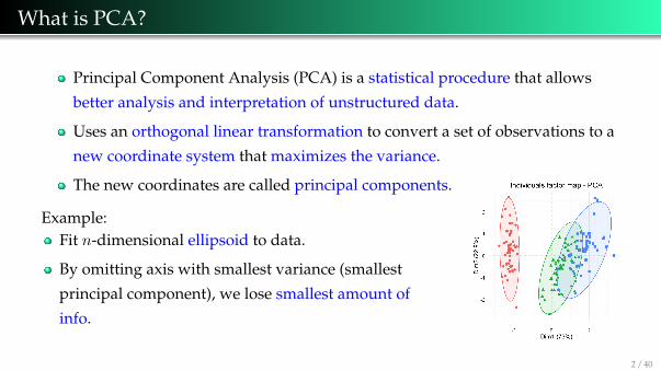
Principal Component Analysis (PCA) is a statistical procedure that allows
better analysis and interpretation of unstructured data.
Uses an orthogonal linear transformation to convert a set of observations to a
new coordinate system that maximizes the variance.
The new coordinates are called principal components.
Example:Fit n-dimensional ellipsoid to data.
By omitting axis with smallest variance (smallest
principal component), we lose smallest amount of
info.
2 / 40

What is PCA?
Principal Component Analysis (PCA) is a statistical procedure that allows
better analysis and interpretation of unstructured data.
Uses an orthogonal linear transformation to convert a set of observations to a
new coordinate system that maximizes the variance.
The new coordinates are called principal components.
Example:Fit n-dimensional ellipsoid to data.
By omitting axis with smallest variance (smallest
principal component), we lose smallest amount of
info.
2 / 40
Principal Component Analysis (PCA) aka...
Signal processing: discrete Kosambi-Karhunen-Loeve transform (KLT)
Multivariate quality control: the Hotelling transform
Mechanical engineering: proper orthogonal decomposition (POD)
Linear algebra: singular value decomposition (SVD) of X (Golub and Van Loan, 1983)
Linear algebra: eigenvalue decomposition (EVD) of XTX
Psychometrics: factor analysis, Eckart-Young theorem (Harman, 1960), or Schmidt-Mirskytheorem
Meteorological science: empirical orthogonal functions (EOF)
Noise and vibration: empirical eigenfunction decomposition (Sirovich, 1987), empiricalcomponent analysis (Lorenz, 1956), quasiharmonic modes (Brooks et al., 1988), spectraldecomposition
Structural dynamics: empirical modal analysis
...
3 / 40

Applications of PCA
Dimension construction
Feature extraction
Data visualization
Image compression
Medical imaging
Lossy data compression
...
4 / 40

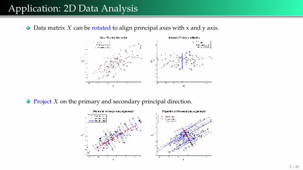
Application: 2D Data Analysis
Data matrix X can be rotated to align principal axes with x and y axis.
Project X on the primary and secondary principal direction.
5 / 40
Application: 2D Data Analysis
Data matrix X can be rotated to align principal axes with x and y axis.
Project X on the primary and secondary principal direction.
5 / 40
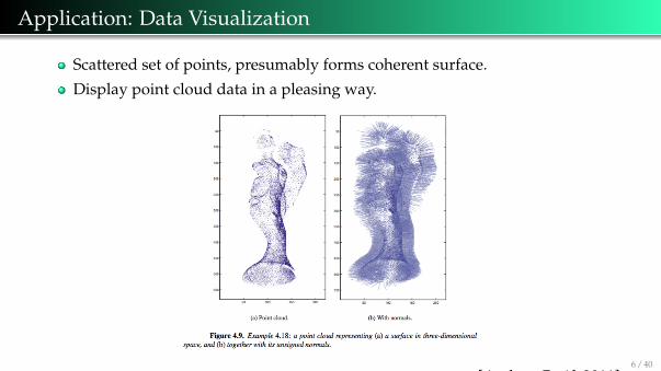
Application: Data Visualization
Scattered set of points, presumably forms coherent surface.
Display point cloud data in a pleasing way.
[Ascher, Greif, 2011]6 / 40

Application: Image Compression
Effectively represent image with limited number of principal components.
Do not know # of principal components needed for successful reconstruction.
7 / 40

Application: Image Compression
Effectively represent image with limited number of principal components.
Do not know # of principal components needed for successful reconstruction.
7 / 40

Application: Image Compression
8 / 40
The Problem
Let X be a D-dimensional random vector with covariance matrix S.
Problem: Consecutively find the unit vectors u1,u2, . . . ,uD such that
Yi = XTui
satisfies:1 var(Y1) is the maximum.2 var(Y2) is the maximum subject to cov(Y2, Y1) = 0.3 var(Yk) is the maximum subject to cov(Yk, Yi) = 0, where k = 3, 4, . . . , D andk > i.
9 / 40
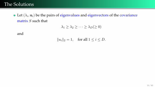
The Solutions
Let (λi,ui) be the pairs of eigenvalues and eigenvectors of the covariance
matrix S such that
λ1 ≥ λ2 ≥ · · · ≥ λD(≥ 0)
and
‖ui‖2 = 1, for all 1 ≤ i ≤ D.
Then var(Yi) = λi for 1 ≤ i ≤ D.
→ The principal components of X are the eigenvectors of S.→ The variance will be a maximum when we set u1 to the eigenvector having the
largest eigenvalue.
→ The proportion of variance each eigenvector represents is given by the ratio of
the given eigenvalue to the sum of all the eigenvalues.
10 / 40

The Solutions
Let (λi,ui) be the pairs of eigenvalues and eigenvectors of the covariance
matrix S such that
λ1 ≥ λ2 ≥ · · · ≥ λD(≥ 0)
and
‖ui‖2 = 1, for all 1 ≤ i ≤ D.
Then var(Yi) = λi for 1 ≤ i ≤ D.
→ The principal components of X are the eigenvectors of S.→ The variance will be a maximum when we set u1 to the eigenvector having the
largest eigenvalue.
→ The proportion of variance each eigenvector represents is given by the ratio of
the given eigenvalue to the sum of all the eigenvalues.10 / 40

Restrictions of PCA
Linear, nonparametric analysis that cannot incorporate prior knowledge.
Important that variance can be used to differentiate/imply similarity.
If the given data set is nonlinear or multimodal distribution, PCA fails to
provide meaningful data reduction.
To incorporate the prior knowledge of data to PCA, researchers haveproposed dimension reduction techniques as extensions of PCA:
e.g., kernel PCA, multilinear PCA, and independent component analysis (ICA).
11 / 40
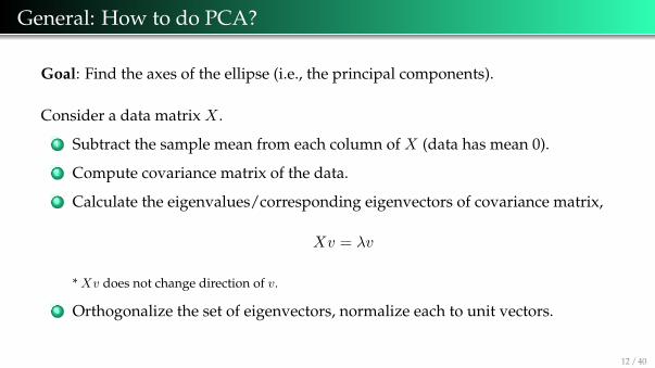
General: How to do PCA?
Goal: Find the axes of the ellipse (i.e., the principal components).
Consider a data matrix X .
1 Subtract the sample mean from each column of X (data has mean 0).
2 Compute covariance matrix of the data.
3 Calculate the eigenvalues/corresponding eigenvectors of covariance matrix,
Xv = λv
* Xv does not change direction of v.
4 Orthogonalize the set of eigenvectors, normalize each to unit vectors.
12 / 40

Formulations of PCA
There are two main formulations of PCA:
Maximum variance formulation: The orthogonal projection of the data onto
a lower dimensional linear space (principal subspace) such that the variance
of the projected data is maximized.
Minimum-error formulation: The linear projection that minimizes the
average projection cost, defined as the mean squared distance between the
data points and their projections.x1
x2
x1
x2
x1
x2
x1
x2
u1 u1
u1u1
13 / 40

Maximum Variance Formulation
Goal: Project data onto space having dimensionality M < D while maximizingvariance of projected data.
Consider a data set of observations {xn}where n = 1, . . . , N .
Each xn is a Euclidean variable with dimensionality D.
Assume projecting onto a one-dimensional space (M = 1).
Define the direction of this space using u1.
Assume u1 is a unit vector (uT1 u1 = 1).
14 / 40

Maximum Variance Formulation
The mean of the projected data is uT1 x where x is the sample set mean
x =1
N
N∑n=1
xn
The variance of the projected data is given by
1
N
N∑n=1
(uT1 xn − uT
1 x)2
= uT1 Su1
where S is the covariance matrix of the data,
S =1
N
N∑n=1
(xn − x)(xn − x)T .
15 / 40

Maximum Variance Formulation
The mean of the projected data is uT1 x where x is the sample set mean
x =1
N
N∑n=1
xn
The variance of the projected data is given by
1
N
N∑n=1
(uT1 xn − uT
1 x)2
= uT1 Su1
where S is the covariance matrix of the data,
S =1
N
N∑n=1
(xn − x)(xn − x)T .
15 / 40
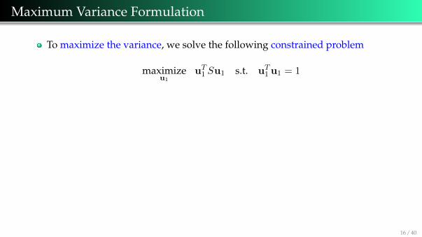
Maximum Variance Formulation
To maximize the variance, we solve the following constrained problem
maximizeu1
uT1 Su1 s.t. uT
1 u1 = 1
The Lagrangian of this problem is given by
L(u1, λ1) = uT1 Su1 + λ1(1− uT
1 u1).
Differentiating with respect to u1, we have a stationary point when
Su1 = λ1u1.
16 / 40
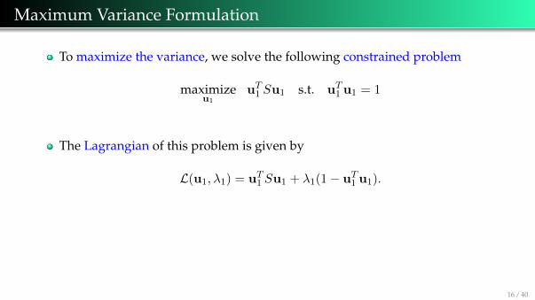

Maximum Variance Formulation
By left-multiplying by u1 and using uT1 u1 = 1, we have
uT1 Su1 = λ1.
Thus, the maximum variance will occur when we set u1 to the eigenvector
having the largest eigenvalue λ1.
Additional principal components can be defined in an incremental fashion.
A similar problem can be formed for the minimum error formulation.
Solution is in terms of the D −M smallest eigenvalues of the eigenvectors thatare orthogonal to the principal subspace.
17 / 40

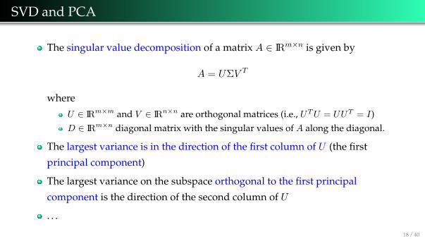
SVD and PCA
The singular value decomposition of a matrix A ∈ IRm×n is given by
A = UΣV T
where
U ∈ IRm×m and V ∈ IRn×n are orthogonal matrices (i.e., UTU = UUT = I)D ∈ IRm×n diagonal matrix with the singular values of A along the diagonal.
The largest variance is in the direction of the first column of U (the first
principal component)
The largest variance on the subspace orthogonal to the first principal
component is the direction of the second column of U
. . .
18 / 40

SVD and PCA
Therefore,
B = UTA = ΣV T
represents a better alignment than the given A in terms of variance
differentiation.
Covariance matrix of A is a positive semi-definite matrix,
C = AAT = UΣΣTUT
and the eigenvectors are the columns of U (namely, the singular vectors
which are the principal components).Application of PCA with respect to SVD:
Solving almost singular linear systemsIf the problem is too ill-conditioned, then regularize it.
19 / 40

SVD and PCA
Therefore,
B = UTA = ΣV T
represents a better alignment than the given A in terms of variance
differentiation.
Covariance matrix of A is a positive semi-definite matrix,
C = AAT = UΣΣTUT
and the eigenvectors are the columns of U (namely, the singular vectors
which are the principal components).
Application of PCA with respect to SVD:Solving almost singular linear systems
If the problem is too ill-conditioned, then regularize it.
19 / 40

SVD and PCA
Therefore,
B = UTA = ΣV T
represents a better alignment than the given A in terms of variance
differentiation.
Covariance matrix of A is a positive semi-definite matrix,
C = AAT = UΣΣTUT
and the eigenvectors are the columns of U (namely, the singular vectors
which are the principal components).Application of PCA with respect to SVD:
Solving almost singular linear systemsIf the problem is too ill-conditioned, then regularize it.
19 / 40
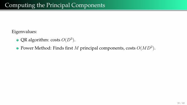
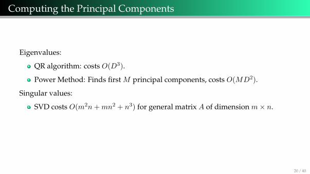
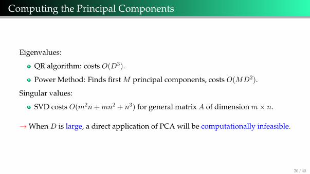
Computing the Principal Components
Eigenvalues:
QR algorithm: costs O(D3).
Power Method: Finds first M principal components, costs O(MD2).
Singular values:
SVD costs O(m2n+mn2 + n3) for general matrix A of dimension m× n.
→When D is large, a direct application of PCA will be computationally infeasible.
20 / 40
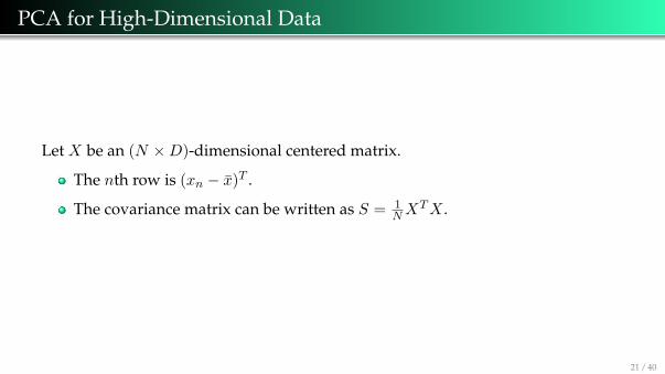
PCA for High-Dimensional Data
Let X be an (N ×D)-dimensional centered matrix.
The nth row is (xn − x)T .
The covariance matrix can be written as S = 1NX
TX .
21 / 40

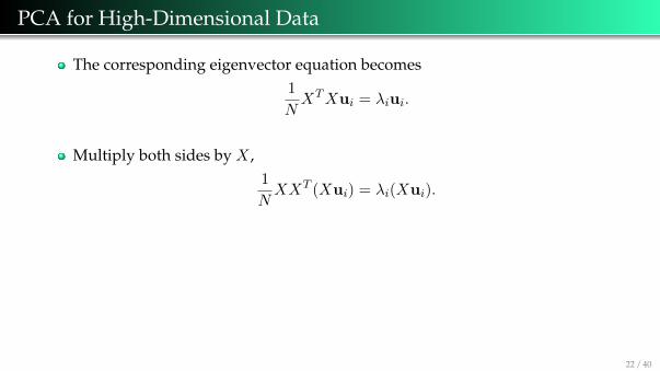
PCA for High-Dimensional Data
The corresponding eigenvector equation becomes1
NXTXui = λiui.
Multiply both sides by X ,1
NXXT (Xui) = λi(Xui).
Let vi = Xui to get1
NXXTvi = λivi,
which is the eigenvector equation for the N ×N matrix 1NXX
T .
This has the same N − 1 eigenvalues as the original covariance matrix.
We can solve the eigenvalue problem for cost of O(N3).
22 / 40

PCA for High-Dimensional Data
The corresponding eigenvector equation becomes1
NXTXui = λiui.
Multiply both sides by X ,1
NXXT (Xui) = λi(Xui).
Let vi = Xui to get1
NXXTvi = λivi,
which is the eigenvector equation for the N ×N matrix 1NXX
T .
This has the same N − 1 eigenvalues as the original covariance matrix.
We can solve the eigenvalue problem for cost of O(N3).22 / 40
Discussion
PCA is a statistical procedure that uses an orthogonal linear transformation to
reduce the dimension of a dataset while maximizing the variance.
PCs of a dataset X are the eigenvectors of its covariance matrix.
Formulated as a maximum variance problem or a minimum error problem.
Transformation for high-dimensional data.
Allows you to find principal components in smaller subspace.
Extensions:Probabilistic PCA
Maximum likelihood PCA, EM algorithm for PCA, Bayesian PCA, Factor analysis
Kernel PCA
23 / 40
Independent Component Analysis
PCA focuses on models with latent variables based on linear-Gaussiandistributions.
The PCs represent a rotation of the coordinate system in data space.Data distribution in the new coordinates is uncorrelated.
This is a necessary condition for independence, but not a sufficient condition.
24 / 40

Independent Component Analysis
PCA focuses on models with latent variables based on linear-Gaussiandistributions.
The PCs represent a rotation of the coordinate system in data space.Data distribution in the new coordinates is uncorrelated.This is a necessary condition for independence, but not a sufficient condition.
24 / 40

Independent Component Analysis
Independent Component Analysis (ICA):
Similar to PCA, finds a new basis to represent data.
Computational method for separating multivariate signal into additivesubcomponents that are maximally independent.Observed variables are linear combination of the latent variables.Assumes subcomponents are non-Gaussian signals and are statisticallyindependent.
25 / 40

Independent Component Analysis
Independent Component Analysis (ICA):
Similar to PCA, finds a new basis to represent data.Computational method for separating multivariate signal into additivesubcomponents that are maximally independent.
Observed variables are linear combination of the latent variables.Assumes subcomponents are non-Gaussian signals and are statisticallyindependent.
25 / 40

Independent Component Analysis
Independent Component Analysis (ICA):
Similar to PCA, finds a new basis to represent data.Computational method for separating multivariate signal into additivesubcomponents that are maximally independent.Observed variables are linear combination of the latent variables.
Assumes subcomponents are non-Gaussian signals and are statisticallyindependent.
25 / 40
Independent Component Analysis
Independent Component Analysis (ICA):
Similar to PCA, finds a new basis to represent data.Computational method for separating multivariate signal into additivesubcomponents that are maximally independent.Observed variables are linear combination of the latent variables.Assumes subcomponents are non-Gaussian signals and are statisticallyindependent.
25 / 40

Example: blind source separation
Example: blind source separation
ICA is used to recover the sources.26 / 40

Example: blind source separation
Consider some data s ∈ IRn that is generated via n independent sources
x = As,
where A is an unknown matrix (mixing matrix), x received signal.
Repeated observations gives a data set {x(i), i = 1, . . . ,m}.
Goal: Recover s(i).
27 / 40
Example: blind source separation
Consider some data s ∈ IRn that is generated via n independent sources
x = As,
where A is an unknown matrix (mixing matrix), x received signal.
Repeated observations gives a data set {x(i), i = 1, . . . ,m}.
Goal: Recover s(i).
27 / 40

Example: blind source separation
Consider some data s ∈ IRn that is generated via n independent sources
x = As,
where A is an unknown matrix (mixing matrix), x received signal.
Repeated observations gives a data set {x(i), i = 1, . . . ,m}.
Goal: Recover s(i).
27 / 40

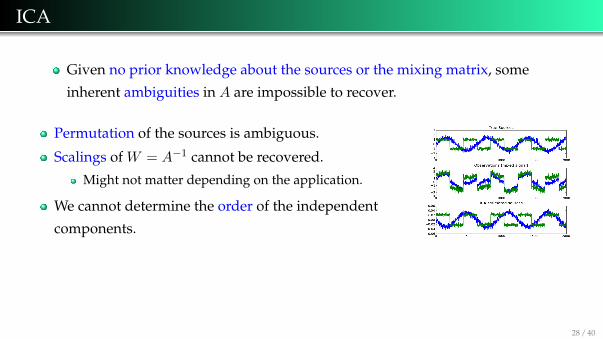
ICA
Given no prior knowledge about the sources or the mixing matrix, some
inherent ambiguities in A are impossible to recover.
Permutation of the sources is ambiguous.
Scalings of W = A−1 cannot be recovered.
Might not matter depending on the application.
We cannot determine the order of the independent
components.
These are the ONLY ambiguities assuming the sources si are non-Gaussian.
As long as the data is non-Gaussian, we can recover the n independent
sources.
28 / 40
ICA Algorithm (Bell and Sejnowski)
Suppose the distribution of each source si is given by a density ps.
The joint distribution of the sources s is given by
p(s) =
n∏i=1
ps(si).
→ By modelling the joint distribution as a product of the marginal, we capture
the assumption that the sources are independent.
This implies the following density on x = As = W−1s :
p(x) =
n∏i=1
ps(wTi x) · |W |.
Need to specify a density for the individual sources ps.
29 / 40

ICA Algorithm (Bell and Sejnowski)
Suppose the distribution of each source si is given by a density ps.
The joint distribution of the sources s is given by
p(s) =
n∏i=1
ps(si).
→ By modelling the joint distribution as a product of the marginal, we capture
the assumption that the sources are independent.
This implies the following density on x = As = W−1s :
p(x) =
n∏i=1
ps(wTi x) · |W |.
Need to specify a density for the individual sources ps.29 / 40

ICA Algorithm
We need to specify a cdf for it that slowly increases from 0 to 1.
Reasonable default: the sigmoid function
g(s) =1
(1 + e−s).
This yields ps(s) = g′(s).
Given a training set {x(i), i = 1, . . . ,m}, the log likelihood for our parameter
matrix W is
`(W ) =m∑i=1
n∑j=1
log g′(wTj x
(i)) + log |W |
.
30 / 40
ICA Algorithm
We need to specify a cdf for it that slowly increases from 0 to 1.
Reasonable default: the sigmoid function
g(s) =1
(1 + e−s).
This yields ps(s) = g′(s).
Given a training set {x(i), i = 1, . . . ,m}, the log likelihood for our parameter
matrix W is
`(W ) =
m∑i=1
n∑j=1
log g′(wTj x
(i)) + log |W |
.
30 / 40

ICA Algorithm
Maximizing this in terms of W , we derive a stochastic gradient ascent
learning rule for training example x(i):
W := W + α
1− 2g(wT
1 x(i))
1− 2g(wT2 x
(i))...
1− 2g(wTnx
(i))
x(i)T
+ (W T )−1
where α is the learning rate.
After the algorithm converges, we compute s(i) = Wx(i) to recover the
original sources.
31 / 40

FastICA Algorithm
FastICA [http://research.ics.aalto.fi/ica/fastica/]
Implements the fast fixed-point algorithm for ICA and projection pursuit.
Can download (for R, C++, Python and Matlab)
32 / 40
FastICA Algorithm
33 / 40

FastICA Algorithm
34 / 40

FastICA Algorithm
35 / 40

FastICA Algorithm
36 / 40
FastICA Algorithm
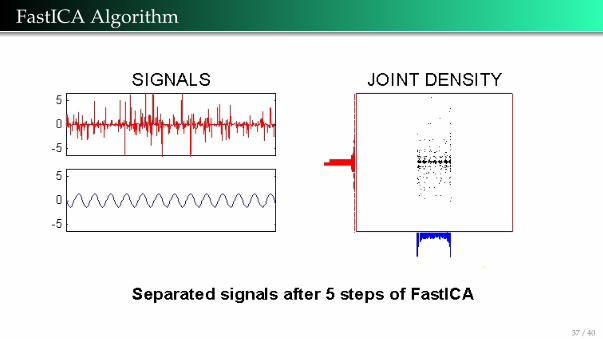
37 / 40

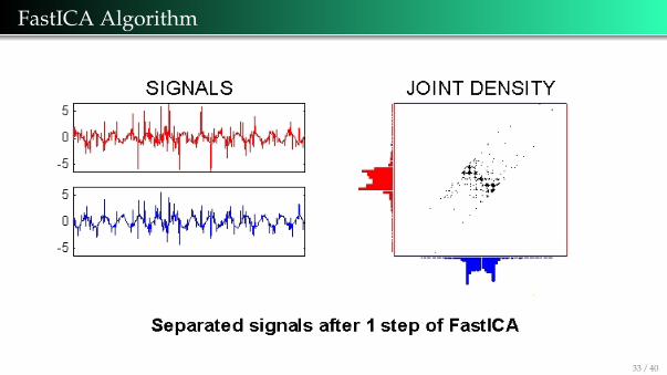
FastICA Algorithm
The source signals were sinusoidal
and impulsive noise.
The joint density is the product ofthe marginal densities.
Definition of independence.
38 / 40

Discussion
ICA is a statistical and computational technique used to reveal hidden factors
that underlie sets of random variables, measurements, or signals.
Data assumed to be linear combinations of some unknown latent variables.
Latent variables are assumed to be non-Gaussian and independent.
ICA finds these independent components.
Stochastic gradient ascent learning rule for training example x(i).
FastICA
. . .
39 / 40
Thank you!
U. M. Ascher and C. Greif, A First Course in Numerical Methods, SIAM, 2011.
C. M. Bishop. Pattern Recognition and Machine Learning, Springer, 2006.
A. Hyvarinen. What is Independent Component Analysis?https://www.cs.helsinki.fi/u/ahyvarin/whatisica.shtml
S. Jang. Basics and Examples of Principal Component Analysis (PCA), slecture, 2014https://www.projectrhea.org/rhea/index.php/PCA_Theory_Examples.
A. Ng. Independent Component Analysis, CS299 Lecture Notes.
FastICA, http://research.ics.aalto.fi/ica/fastica/.
40 / 40


![Consolidation of Unorganized Point Clouds for Surface …ascher/papers/hlzac.pdf · 2009. 8. 31. · predictor-corrector scheme (see [Ascher and Petzold 1998] for ori-gins and analogies](https://static.documents.pub/doc/80x56/61042ad1ca767d7f2c473345/consolidation-of-unorganized-point-clouds-for-surface-ascherpapershlzacpdf.jpg)


