Analysis of mesh models is gaining prominence as it has wide range of applications from engineering to medicine. In this paper, we present a method for analyzing meshes through the abstraction of its prominent cross-sections (PCS). An algorithm that can robustly yield prominent cross-section at any point on the mesh that approximates the local sweep has been presented. Two types of prominent cross-sections, full (FPCS) and partial (PPCS) are defined and computed over the model. These cross-sections, that cover the object, can then be used in further analysis. Skeleton computation and shape matching using prominent cross-sections have been demonstrated.
Analysis and representation of meshes is gaining prominence as it is useful in understanding 3D shape content. Mesh model analysis has been prominently used for segmentation and is broadly classified as surface-based and part-based methods. Most of the surface-based methods, in particular region growing and watershed methods, use various forms of curvature, dihedral angle or surface normals to identify the types of surfaces the regions represent. The part-based methods such as reeb graphs uses height function or geodesic distance to construct a skeleton by identifying the convex or concave regions to segment the object into parts. For a detailed review please see [2], [5] and [36]. These methods typically cater to only a particular application such as segmentation, skeletonization or search. More recently, volume-based methods are being used to explore the mesh models such as for search [37] and for skeletonization [6]. It is important to derive a meaningful representation that captures geometry and topology of the mesh to understand the shape to support multiple applications.
Meshes represent complex objects in a discrete form and hence identifying local shape features in a complex mesh model is a difficult task. Although a lot of work has been done for local analysis of
meshes ([25], [28], [37]), the local representation does not support global reasoning. On the other hand global analysis ([14], [20], [23], [29]), and their representations do not capture the local shape. The challenges in the understanding of meshes arise because the local methods do not capture the global characteristics and global representations lose local knowledge. Additional difficulties are caused because the representation arising from mesh model analysis have to be invariant to model articulation, deformation, geometrical and topological noise.
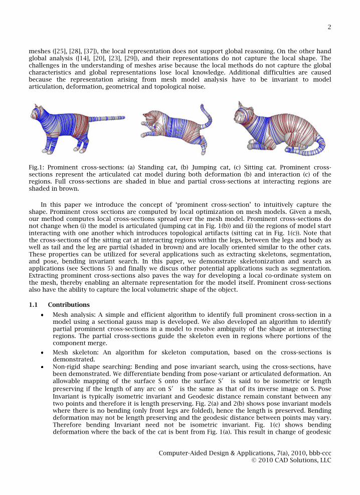
Fig.1: Prominent cross-sections: (a) Standing cat, (b) Jumping cat, (c) Sitting cat. Prominent cross-sections represent the articulated cat model during both deformation (b) and interaction (c) of the regions. Full cross-sections are shaded in blue and partial cross-sections at interacting regions are shaded in brown.
In this paper we introduce the concept of ‘prominent cross-section’ to intuitively capture the
shape. Prominent cross sections are computed by local optimization on mesh models. Given a mesh, our method computes local cross-sections spread over the mesh model. Prominent cross-sections do not change when (i) the model is articulated (jumping cat in Fig. 1(b)) and (ii) the regions of model start interacting with one another which introduces topological artifacts (sitting cat in Fig. 1(c)). Note that the cross-sections of the sitting cat at interacting regions within the legs, between the legs and body as well as tail and the leg are partial (shaded in brown) and are locally oriented similar to the other cats. These properties can be utilized for several applications such as extracting skeletons, segmentation, and pose, bending invariant search. In this paper, we demonstrate skeletonization and search as applications (see Sections 5) and finally we discus other potential applications such as segmentation. Extracting prominent cross-sections also paves the way for developing a local co-ordinate system on the mesh, thereby enabling an alternate representation for the model itself. Prominent cross-sections also have the ability to capture the local volumetric shape of the object.
1.1 Contributions
Mesh analysis: A simple and efficient algorithm to identify full prominent cross-section in a model using a sectional gauss map is developed. We also developed an algorithm to identify partial prominent cross-sections in a model to resolve ambiguity of the shape at intersecting regions. The partial cross-sections guide the skeleton even in regions where portions of the component merge.
Mesh skeleton: An algorithm for skeleton computation, based on the cross-sections is demonstrated.
Non-rigid shape searching: Bending and pose invariant search, using the cross-sections, have been demonstrated. We differentiate bending from pose-variant or articulated deformation. An allowable mapping of the surface S onto the surface S′ is said to be isometric or length
preserving if the length of any arc on S′ is the same as that of its inverse image on S. Pose
Invariant is typically isometric invariant and Geodesic distance remain constant between any two points and therefore it is length preserving. Fig. 2(a) and 2(b) shows pose invariant models where there is no bending (only front legs are folded), hence the length is preserved. Bending deformation may not be length preserving and the geodesic distance between points may vary. Therefore bending Invariant need not be isometric invariant. Fig. 1(c) shows bending deformation where the back of the cat is bent from Fig. 1(a). This result in change of geodesic
distance between any two points and hence the length is not preserved in these two variants of cat models
2 RELATED WORK
In the previous section, we have reviewed shape analysis. We demonstrate skeletonization and shape searching to illustrate the potential uses of the proposed representation. Hence, we provide a review of related work in the context of the skeletonization and search in the following sections.
2.1 Skeletonization
Li et al. [26] and Mortara et al. [28] have proposed to decompose a mesh using the cross-sections of the mesh. Li et al. [26] used space sweeping with predefined sweep paths (similar to skeletons), obtained by edge contraction [18] of the mesh model to identify cross-sections. Plumber [28] uses the intersection of sphere with the mesh to generate generalized cylinders or cones. Recent curve-skeleton generation methods have adopted approaches such as approximate medial computation and refining [12], decomposition [27], reconstruction [38] and shape diameter function [37]. For a detailed review of various skeletons, refer to [10]. The main difficulty in computing curve-skeletons for complex objects is to correctly interpret their shape and this requires a robust and accurate interpretation mechanism [38]. In contrast, our approach does not require predefined sweep paths and generates cross-section that are planar. We also address the cross-sections at the ambiguous regions of intersections.
To construct skeletons, most of the prior work on meshes has predominantly dealt with operations on the mesh model directly. In contrast to the existing approaches, we propose to use the prominent cross-sections to generate skeletons as they can be computed robustly and efficiently. Our approach uses full prominent cross-sections and partial prominent cross sections that characterize the local shape of the object, to evolve the skeleton of the object.
2.2 Shape Search
Most of the state-of-the-art approaches deal with only rigid shape matching. Global feature-based methods use global properties of the model such as moment invariants [11], fourier descriptors [35], [30] and geometric ratios [32]. Histograms [4], [24] and shape distributions [31], [29] use properties such as distance, angle, area and volume between random points on the model. Light-field descriptor (LFD) [9], a view-based method, has been shown to give very good retrieval results for rigid matching. Graph-based methods such as Reeb graph [17], [7] are hard, slow, complex and susceptible to topology changes, in general.
Diameter shape-function [16] has been shown to be invariant to various poses of the model. Bending-invariant representation based on multidimensional scaling has been presented in [13]. This method, has shown to be too sensitive to modifications and hard to control on general 3D meshes [16]. Recent approaches [21], [34] for non-rigid matching have used the concepts from manifold learning. The utility of these methods depend upon the quality of the descriptors which enter into the construction of the affinity matrices [20]. Research on partial shape matching using features has been the topic of [14], [15]. A detailed review of various shape descriptors for 3D model retrieval can be found in [40] and [19].
Fig. 2: Similar signatures are obtained based on the cross-sections for pose invariant lion models.
Computing prominent cross-sections can be efficiently used in bending/pose invariant shape matching. Figure 1 shows cross-sections on cat models that are bending/scaling variants of each other. The cross-sections are similar in these models. They are not sensitive to any deformation that does not change the volumetric shape locally such as articulated deformations, rigid transformations and bending. In this paper, it is shown that prominent cross-sections can be used to obtain shape functions that are effective in retrieving not only pose-invariant (articulated) models but also bending-invariant ones. Figures 2(c) and 2(d) show signatures of pose-invariant lion models obtained by defining a shape function based on cross sections (for details, refer to Section 5.2).
3 COMPUTING A PROMINENT CROSS-SECTION: THEORY AND ALGORITHM
3.1 Computing Cross-sections using sectional Gauss map
In this section, computing the prominent cross-section (PCS) at a point on the model is described. PCS at a point can be defined as a cross-section of a local sweep (with or without scaling) passing through that point. Figure 3(a) shows two points P1 and P2 and their corresponding PCS: C1 and C2 on a given hyperboloid. In this case PCS is unique, but for closed surfaces like sphere or ellipsoid there can be more than one PCS that corresponds to any given point on the surface.
Fig.3: (a) PCS on Hyperbloid, (b) and (c) Sectional Gauss Map for Cross-sections on a model.
Let N be the normal to the surface at a point X. The map N: XR3 takes its values in the unit sphere [8].
S2 = {(x,y,z) ε R3 | x2+y2+z2 = 1}
The map N: X S2, thus defined is called the Local Gauss Map. The Gauss map constructed for the normals of facets from a section is called the Sectional Gauss Map. The construction is as follows: the plane normal (Np) is placed at the pole of the sphere. The normal of the facet is plotted on the unit sphere using the angle between each normal of a facet and Np. Figures 3(b) and 3(c) show sectional Gauss maps (red indicates the pole of the sphere, the green are the normals from the facets of intersection of the plane with the mesh). Let Ni be the set of facet normals, obtained by the intersection with the plane P1 or P2 and the hyperboloid. The normals Ni may not lie on the cross-section plane, in general (as in case of P2). In other words, they may not be perpendicular to the normal Np of the cross-section plane. For a reasonable cross-section (correspond to a smooth local sweep), one can assume the following:
∀ n ε Ni, n. Np = c
When c = 0, the normals Ni pass through cross-section plane (as in case of P1).
Proposition 1: Ni’s lie on a latitude (or parallel to the latitude) of the sectional gauss map.
The proof is straight forward to see as it comes from n.Np = c (or c = 0). Figure3(b) shows the sectional Gauss map where the normals lie on the latitude corresponds to PCS C1 and Figure 3(c) shows the map when it is parallel to the latitude which corresponds to PCS C2 in Figure 3(a). Proposition 1 paves the way for an algorithm to compute the prominent cross-sections. For obtaining the correct orientation of the cross-sectional plane, the normals Ni, are plotted in the sectional gauss map, with respect to the plane normal Np and optimized in the Gauss map itself.
3.2 Algorithm Description
The aim is to compute the cross section plane passing through a given vertex in the mesh. The normals in the mesh are computed using [33], which allows computing them at a non-vertex location using interpolation of the explicitly computed second fundamental form at the vertices. The algorithm begins by taking an initial plane passing through the given vertex. The intersection of the plane through the one-ring neighborhood is calculated and propagated until the complete loop is computed. The normals at the intersection of the cross section plane and the mesh edges are obtained by interpolating the corresponding vertex normal linearly. Then the sectional gauss map is constructed. This plots the relative orientation of the intersection normals with the cross section plane normal. Further these normals are analyzed on the gauss map.
Initial Planes: The initial plane is obtained from the Frenet trihedron at the given point. Either Kmin × N or Kmax × N, where N is a normal at a point in the model, can be used as initial cross-sectional plane.
Optimization, stabilizing and formation of a prominent cross-section: The optimization of plane orientation requires normals of intersecting facets. From a given point on the mesh, a facet is checked to determine whether it intersects with current plane to include in facet normals set (Ni). Intersection points are not required for optimization. In this work, the mesh model is stored in a winged edge data structure, implemented in CGAL [1]. The intersection of the plane through the one ring neighborhood is calculated for the given point pi. If the given point is a vertex on the mesh, the starting intersection will yield two edges or two vertices or one vertex and one edge. If the result is an edge, the next interesting facet is obtained by querying the opposite halfedge. If the result is a vertex, again a one-ring neighborhood is computed to identify corresponding facet. This process is repeated until the full cross-section is computed by reaching the starting point (pi).
Then, the sectional gauss map is constructed by the mapping facet normals on the unit sphere. This plots the relative orientation of the intersection normals with the cross-section plane normal. Proposition 1 implies that the normals lie on the greater circle or parallel to the great circle. However, due to a discrete representation, the normals need to be approximated. Hence, identifying the cross
Algorithm 1 ComputeCrossSections(Mesh)
for a point pi ε sampled points do
Plane = Identify starting plane (P) at point (pi)
repeat Identify point normals N
i which intersect with (P)
Plot point normals Ni on Sectional Gauss map
P = Find best fit plane on the Gauss map until The best fit plane converges to threshold Generate PCS using P at the point (p
sectional plane is similar to finding the best fit plane on the Gauss map. The best plane is obtained by least-square fitting. The newly obtained plane orientation is compared with ideal plane orientation (the one passes through the pole of the unit sphere). The above process is repeated until the best plane and pole coincide within user specified threshold (1e-6). Finally, points on the cross-section are computed using edge (line) and plane intersection.
Fig. 4: Prominent cross-section plane at a point on the dragon Figures 4(a) and 4(b) shows the initial cross-section (loop) and the corresponding section Gauss map. The cross-section and the sectional Gauss map after a few iterations are shown in Figures 4(c) and 4(d). Figure 4(d) shows that the normal (in blue) of the best fit plane is moving towards the direction of the pole (in red). Figure 4(e) shows the final (prominent) cross-section plane and the computed loop.
3.3 Robustness
Fig.5: Illustration of robustness - prominent cross-section is computed for a model spread with Gaussian noise. (a),(b) - 2% noise, (C),(d) - 5% noise, (e),(f) - 10%, (g),(h) - 20% noise To analyze the robustness of the algorithm, we introduced Gaussian noise of various levels in the model and tested for cross-section stabilization. Figure 5 shows the sectional Gauss map and the cross sections for a model with Gaussian noise of 2%, 5%, 10% and 20%. The initial cross-section stabilizes in a few iterations. Even when the noise is high (for example, 20%), the cross section gets stabilized
though the normals in the map (refer to the associated sectional Gauss map (Figure 5(g)). The convergence of the algorithm was tested on various models. For most of the models, the optimization procedure to obtain a prominent cross-section converged within ten iterations. For the dragon, a very complex model with noise, it took a bit longer (sometimes 25 iterations) to converge. For most of the cases, the convergence took place in less than a second. Even when the algorithm took more iterations, the time taken is less than a second. Hence, the algorithm is robust, and fast.
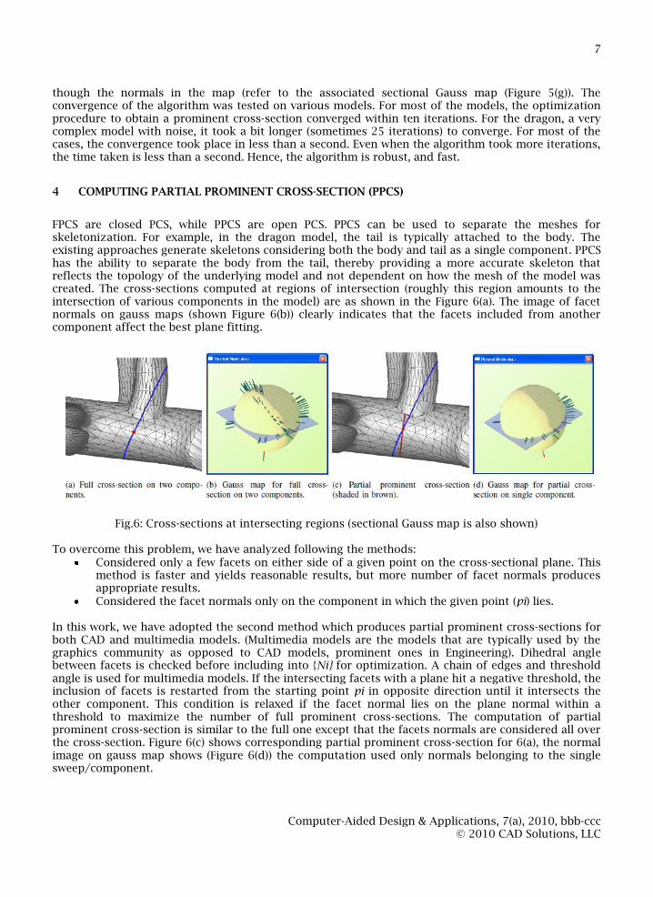
FPCS are closed PCS, while PPCS are open PCS. PPCS can be used to separate the meshes for skeletonization. For example, in the dragon model, the tail is typically attached to the body. The existing approaches generate skeletons considering both the body and tail as a single component. PPCS has the ability to separate the body from the tail, thereby providing a more accurate skeleton that reflects the topology of the underlying model and not dependent on how the mesh of the model was created. The cross-sections computed at regions of intersection (roughly this region amounts to the intersection of various components in the model) are as shown in the Figure 6(a). The image of facet normals on gauss maps (shown Figure 6(b)) clearly indicates that the facets included from another component affect the best plane fitting.
Fig.6: Cross-sections at intersecting regions (sectional Gauss map is also shown) To overcome this problem, we have analyzed following the methods:
Considered only a few facets on either side of a given point on the cross-sectional plane. This method is faster and yields reasonable results, but more number of facet normals produces appropriate results.
Considered the facet normals only on the component in which the given point (pi) lies. In this work, we have adopted the second method which produces partial prominent cross-sections for both CAD and multimedia models. (Multimedia models are the models that are typically used by the graphics community as opposed to CAD models, prominent ones in Engineering). Dihedral angle between facets is checked before including into {Ni} for optimization. A chain of edges and threshold angle is used for multimedia models. If the intersecting facets with a plane hit a negative threshold, the inclusion of facets is restarted from the starting point pi in opposite direction until it intersects the other component. This condition is relaxed if the facet normal lies on the plane normal within a threshold to maximize the number of full prominent cross-sections. The computation of partial prominent cross-section is similar to the full one except that the facets normals are considered all over the cross-section. Figure 6(c) shows corresponding partial prominent cross-section for 6(a), the normal image on gauss map shows (Figure 6(d)) the computation used only normals belonging to the single sweep/component.
4.1 Generating full and partial prominent cross-sections
Initially, prominent cross-sections are generated from sampling of the vertices in the model. Currently, a curvature-based sampling has been used. The generated prominent cross-sections using sampling only took few seconds (less than 30sec) for most models. One notable aspect is that the cross-sections get generated in the regions of intersection (of various approximately swept portions of the model) as well. Swept volume is a solid obtained by sweeping a cross-section through space. This is very useful for handling intersection regions as opposed to using an artifact between skeletal portions of the edge contraction applied in [26]. Moreover, the prominent cross-sections have been spread all over the model.
Fig. 7: (a) T-joint model, (b) Twisted tree model. Full (shaded in blue) and partial (shaded in brown) prominent cross-sections for intersecting swept volumes. Figures 7(a) and 7(b) show full and partial prominent cross-sections for CAD models. Figure 8 shows prominent cross sections for multimedia models. Most of the multimedia models are obtained from AIM@Shape shape repository ([3]). The results show that the prominent cross-sections can be computed for both CAD as well as multimedia models. Moreover, it is shown that they can be computed for a model with noise as well. The dot product threshold between plane normal and facet normal is 0.025. The threshold for dihedral angle used in computing the partial prominent cross-sections is -20 degrees.
However, the same dihedral threshold may not be applicable for models with noise. In the future, grouping of normals on Gauss sphere will be employed to handle noise in the model. Generating prominent cross-sections, in addition to complementing the existing advantages, can also overcome the deficiencies currently present in some of the applications. For example, in mesh decomposition, typical advantages such as hierarchical/multi scale decomposition, insensitivity to pose and defining various control parameters can be achieved with the generated prominent cross-sections. However, they provide different set of control parameters in addition to the typically used one such as scaling and area of the sections. Using them enables the mesh to be decomposed volumetrically. Sweep parameters such as path and transformation matrix (linear transformation between prominent cross-sections) can be computed. In addition, the real strength of the prominent cross-sections lies in partial prominent cross-sections, a very useful entity in separating out regions that are joined together in a mesh model.
Fig.8: Prominent cross-sections for mesh models. (a) Horse, (b) Dino, (c) Dog, (d) Dragon, (e) Octopus, (f) hand, (g) Fertility, (h) Elk. Full cross-sections are shaded in blue and partial cross-sections at interacting regions are shaded in brown.
Applications such as editing, animation, morphing or shape matching often need a higher level understanding of the shape and its structure. Such an understanding can be conveyed through the use of a curve-skeleton, an abstract geometrical and topological representation of its 3D shape. They are thinned 1D representation of 3D objects. Moreover, curve-skeleton is easier to handle than the medial axis since it avoids surface elements, while its topological structure still represents the shape efficiently.
The algorithm to generate the skeleton uses the computed cross-sections, both partial and full. In
order to compute the skeleton of the model, we group cross-sections belonging to the same swept volume and compute the corresponding skeleton for the sweep. While grouping the cross-sections, interacting sweeps are identified and skeletons of swept volumes are merged. Algorithm 2 describes a high-level procedure for generating the skeleton using the cross-sections.
5.1.1 Cross-sections clustering to identify swept volume
The algorithm starts by picking a seed cross-section arbitrarily. By grouping of facets from the seed cross-section on both the directions of the seed plane, all the cross-sections belongs to a swept volume are identified. Initially, facets underlying the seed cross-section are grouped. Using the facet adjacency relationship (model is stored in winged edge data-structure), neighbor facets are grouped. While grouping, facets are checked for new cross-section which is intersecting. If a new cross-section is encountered, comparison between current cross-section and newly identified cross-section is performed to check whether they belong to same swept volume. The following criteria are used to identify the cross-section belonging to same swept volume:
angle between cross-sections area and perimeter of the cross-sections and radius of cross-section.
The Radius of the cross-section is computed from three non-collinear points on the cross-section. This enables computing radius even for partial cross-section. Termination of the clustering is based on the cross-section matching or no cross-section is encountered while grouping the cross-sections.
5.1.2 Computing skeleton points
Initially, the centroid of each loop is computed and used as possible skeleton points on each of the loop. As the full loops are planar and closed, we obtain polygons. Hence, computing the centroid of a cross-section amounts to identifying the centroid of a polygon. For a partial cross-section, an approximate centroid is computed in a similar fashion. These points also ensure that the skeleton remains thin, a property that a skeleton [10] has to satisfy. Finally, the smooth skeleton is achieved by spline fitting.
5.1.3 Merging the swept volume skeletons
The individual skeleton of swept volumes is merged to obtain the final skeleton. Swept volume identifier is stored in each facet belonging to it. While grouping the facets during cross-section clustering, the adjacent facets are queried for its swept volume. If the adjacent facet belongs to different swept volume, the adjacent swept volume identifier is noted and merging of the corresponding skeletons are performed at the end of the each clustering process.
Algorithm 2 Skeleton (Cross-section)
Pick randomly a seed cross-section. Cluster neighboring cross-sections bi-directionally. Compute skeleton of swept volume. Merge interacting skeletons
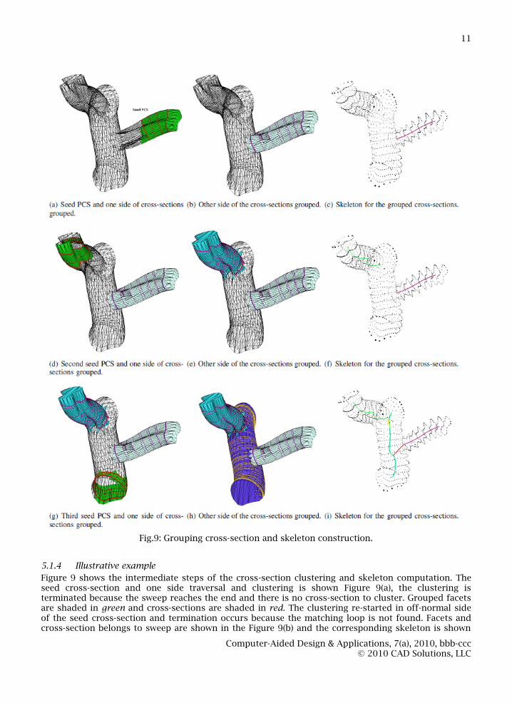
Fig.9: Grouping cross-section and skeleton construction.
5.1.4 Illustrative example
Figure 9 shows the intermediate steps of the cross-section clustering and skeleton computation. The seed cross-section and one side traversal and clustering is shown Figure 9(a), the clustering is terminated because the sweep reaches the end and there is no cross-section to cluster. Grouped facets are shaded in green and cross-sections are shaded in red. The clustering re-started in off-normal side of the seed cross-section and termination occurs because the matching loop is not found. Facets and cross-section belongs to sweep are shown in the Figure 9(b) and the corresponding skeleton is shown
in Figure 9(c). The clustering process is continued with the new seed cross-section and corresponding sweep segments and skeleton are shown in the Figures 9(d-i). The skeleton merging is shown in Figure 9(i). Partial prominent cross-sections are taken into account while clustering the cross-sections; PPCS helps growing the skeleton across the regions of sweep intersections. For example, the center swept volume is identified as single sweep as shown in the Figure 9(h). Figure 10 shows the grouped cross-sections and corresponding skeletons.
5.2 Shape Matching: Cross-sections as a tool for shape function
The key idea is to use a local geometric derivative, cross-sections, to formulate shape functions that can then be used to compute shape signatures. The shape signature can be obtained either by using a histogram of the shape function or using a probability distribution function as in [31]. To compute the shape signature, sampling of points on the mesh is used. The dissimilarity between objects can then evaluated using a metric such as L
N norm. The approach is illustrated in Algorithm 3. This approach
also satisfies the following properties that a shape matching method requires:
Rigid-invariance: Rotation-invariancy is easy to see as the cross-sections are invariant under rotation. Scaling-invariancy can be obtained by normalizing.
Robustness: It is achieved by using sampling. Metric: It comes from the properties of the norm used in the similarity measurement.
However, in contrast to most of the other approaches, we also obtain signatures that are bending invariant as the cross-sections are invariant to bending. The current approaches, based on either geodesic distance computation [13] have been shown to be too sensitive, or the diameter function (DF) [16], though shown to be pose-invariant, is not designed to be bending invariant. This is because, the DF values at a point will differ before and after bending.
5.2.1 Choosing a shape function
The properties of the computed prominent cross-sections are used to define shape function. FPCS is used to define shape function as the cross-section can be considered to define properties of the surface attributes locally. Possible parameters for shape functions are area of the cross-sections, normals of the cross-sections that will provide the orientation locally, and distance between the cross-sections. For simplicity, we focus only on the following measurements of the FPCS - area of a cross-section, which captures the geometric property and average central distance of each cross-section, which can be considered to capture the local shape of the cross-section, as our initial shape functions for experimentation. Currently, we only employ FPCS to compute the shape function. We do not take into account the details of PPCS. Note that the functions are easy to compute and is invariant to rigid transformations.
5.2.2 Shape signatures
To obtain a shape signature based on the cross-sections, we compute the following: Normalized cross-sectional area (NCSA). Normalized central distance of cross-section (NCD).
Algorithm 3 Shape Matching (Mesh) for Each query/database model do
Generate sample points on Mesh S. Compute the cross-sections for each point pi ε S using Algorithm 1 Compute shape function. Compute the Histogram/Distribution.
Initially, sampling is used to generate FPCS in the models. NCSA is obtained by dividing all the FPCS with the Maximum FPCS (FPCSmax). FPCSmax is the largest FPCS, in terms of area of the FPCS. Each FPCS in the shape signature NCSA will then contain the approximated probability value for the FPCS. NCSA can then be viewed as a histogram. The number of bins for generating the histogram is chosen as 64. Figure 12 shows that, for similar models, the histogram of the approximated probability values are similar (also see Figure 2, where the signatures for lion models are shown). The figure shows the results for cat and elephant models, which are essentially pose-variant models and also for models made of intersecting pipes, which are bending variants of each other, created using a modeler. Note that the signature NCSA is similar for bending-variant models. Moreover, for different classes, signatures are also different. For example, the elephant and cat models belong to different classes and the histogram is dissimilar. Similar signatures are also obtained using NCD through a similar procedure.
Fig. 10: Grouping Cross-sections and their skeletons. (a, b) Horse, (c, d) Dino, (e, f) Dog, (g, h) Hand, (i, j) Elk and (k, l) Fertility.
’Central distance’ is defined as the distance between centroid of each cross-section and a point on the FPCS. To compute the NCD, sample points (essentially, they are the intersection points computed during the cross-sections) are used on the cross-section and then averaged out and normalized across all cross-sections. The dissimilarity is captured by the cross-sections and their signatures from NCSA and NCD are also different. This is because the cross-sections largely remain consistent when there is change of pose/bending. In short, signatures using cross-sections (NCSA and NCD) have the ability to capture not only pose-variant but also bending-variants. Another common signature, the D2 (distance between two random points [31]) distribution for the same number of sample points (of the vertices) is also shown in the Figure 11. Also, it should be noted that the shape signatures- NCSA and NCD do not contain the spatial information. The spatial information can be augmented using a distance function between cross-sections (which essentially remains same if the length of the articulations are maintained consistent), similar to the centricity function using in [16].
Fig.11: Similar signatures are obtained for models in the same class. Figure shows Model, NCSA, NCD and D2 in that order for few models.
5.2.3 Sampling
One crucial factor in shape matching technique adopted in this paper is sampling, as FPCS computation for each vertex on the model could be expensive. A robust sampling that can capture both spatial distribution and its local geometry information using FPCS consistently is difficult to obtain, in general. Hence, to compute the shape function and the shape signatures NCSA and NCD, FPCS computation was tested with curvature, random and uniform sampling. We found that uniform sampling performed better, although this calls for further investigation. Moreover, choosing the number of samples is also critical. However, there is a tradeoff here as large samples can increase
the computation time although they can provide more accurate results. For the uniform sampling, we found that 1000 samples produces good results for both NCSA and NCD. Choosing number of samples and the sampling itself needs further investigation.
5.2.4 Qualitative Performance
In the following discussions, only the signature NCSA is discussed, unless otherwise mentioned. To test for robustness with respect to noise, Gaussian noise of the order of 2%, 5%, and 10% is introduced in a model and then the signature is obtained. Figure 12 shows the signatures of the noisy models. It can be seen that the signatures largely remain consistent. This is attributed to the fact that the PCS computation has shown to produce largely consistent cross-sections for noisy models (refer Section 3.3).
To retrieve similar models from a database, shape signatures are usually indexed that enables faster retrievals. However, a distance measure between two signatures has to be defined. Given two functions, its similarity can be computed using the following using measures such as X2, and Minkowski’s LN, among various other measures (see for example [19]). We essentially used L2 norm as the distance measure to retrieve similar models from a database.
The database that is used to compare is similar to ISDB, consisting of various different articulated models of animals such as horse, elephant, cats and lions. It should be noted that, most of the models come under the category of articulated variants. Hence, to test our approach, we also added bending variants of a model. We included couple of classes of models to the database. A three pipe-like intersection, having complex variation of transformation along the spine of the model (a construction typical to CAD models) and its bending variants are added to the database. Another class consists of bending variant models whose cross-section are similar to I-section. Some of the models have noise present in them - for example, the horse models. Essentially, the database is a combination of articulated models of ISDB and the bend variant models that we have created. We term it as PBD - Pose-Bend database. Also, each model may have different number of facets. The approach in this paper has the potential to deal with not only single manifold models but also models having cracks and missing polygons. As we use only FPCS, the models that are tested are closed manifold models.
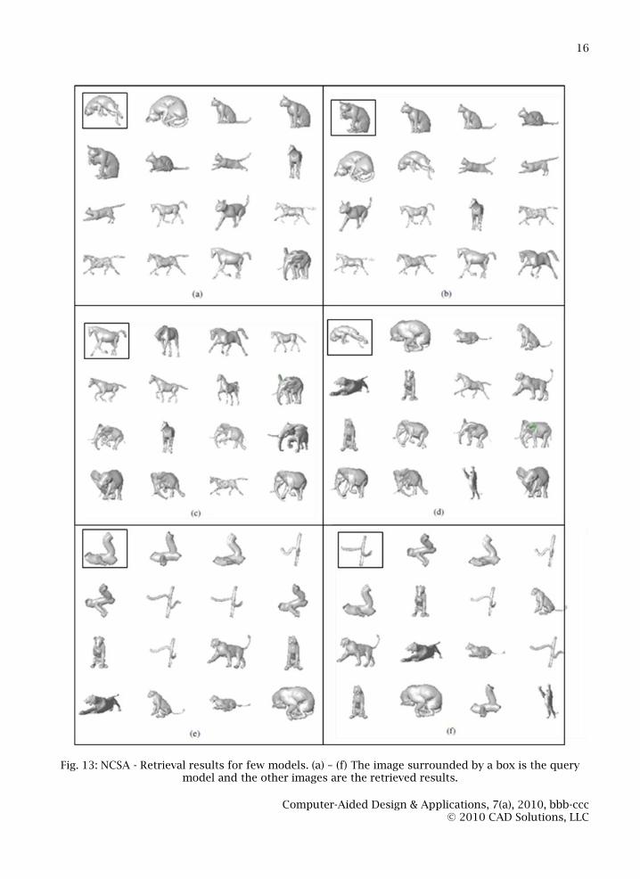
Fig.12: NCSA - Similar signatures are obtained for noisy models added using Guassian noise. 0%, 2%, 5%, and 10% noise modes and their respective NCSA are shown. Figure 13 shows the retrieval results for a few models. The query model is the first model (which is also a retrieved model). The first sixteen retrievals are shown in the figure for each model. Note that the approach works for both bend-variant (see for example Figure 13(a) and Figure 13(e)) as well as pose-variant models (Figure 13(b). In the retrieval of the horse model (Figure 13(c)), the noisy model (see the last row) is also retrieved, which shows that this approach is robust to noisy models. However, we did not test for the bounds on the percentage of noise for which the retrieval is effective. In Figures 13(e) and 13(f), the retrieved models (similar to the query model) are not only bending variants but also the length of each portion is different and the approach was not dependant on the length.
Fig. 13: NCSA - Retrieval results for few models. (a) – (f) The image surrounded by a box is the query model and the other images are the retrieved results.
In addition to the qualitative visualizations of retrieval results, we also evaluate retrieval performance by calculating various quantitative statistics based on the parameters described in [39]. Specifically, we used mean first and second tier measures. The measurements are briefly described here.
5.3.1 First and Second Tier Evaluation
First-tier and second-tier values are defined as percentage of models in the query’s class that appear in top K matches, where K is dependent on the size of the query’s class. The higher values of these statistics indicate better retrieval results. It should be noted that evaluating the results on any database strongly depends on the definition of the classes and the number of models in each class. In our database, though the number of models is small, it has both noisy models as well as variation in length of articulation. In this context, the numbers in the Table 1 are comparable to the descriptors that are specialized for pose-invariancy [16].
Model First Tier % Second Tier %
Cat(9) 87.78 90
Elephant (10) 87 100
Horse (13) 62.3 100
Lion (9) 78.87 87.78
Pipe (10) 71 85
Table 1. Mean First and Second tier statistics for few models.
6 DISCUSSION
Although we have developed a new method for computing prominent cross-sections, organizing and performing operation using them, we see a number of further improvements can be made and new insights be developed.
6.1 Sampling
In the current work, we have used k-mean clustering [22] on vertices of the mesh to obtain uniform sampling. However, this sampling technique is surface based and it is likely that there will be multiple sampling points on a single cross-section. Developing sampling techniques which are volume-aware can address some of these issues.
6.2 Computation of stable partial cross-section
Dihedral angle-based technique for terminating the growth of partial prominent cross-section does not robustly handle the noise in the mesh. To handle the noise we can consider grouping of the normals on the Gauss sphere.
6.3 Shape search
In this paper, we have experimented with the area of cross-sections and the average central distance of each cross-section. The structural information such as distances between the cross-sections along the skeleton can be used to enhance the representation for search. Also, a hierarchical classification of the cross-sections based on the radius of the cross-sections adds an advantage to shape search. We have calculated the equivalent radius of the partial cross-section by choosing three points on the crosssection. We have generated histogram for radius of the cross-sections and the bins are colored from green to red (shown in Figure 14(b) and 14(d). Figures 14(a) and 14(c) show the classified of cross-sections of articulated cat models. Note that the partial cross-sections of sitting cat and full cross-
sections of the standing cat on the body falls in the same color range. This observation enables potential for correspondences as well as hierarchical representations.
Fig. 14: Hierarchical classification of prominent cross-sections for shape search.
6.4 Segmentation
Figure 15 shows part-based segmentation for two models. The segmentation at interacting regions is well separated and will be useful for topological editing. In the present work, the segmentation of model is only shown to illustrate the potential. These initial results were obtained as by product of the skeleton construction.
Fig. 15: Mesh Segmentation using prominent cross-sections.
7 CONCLUSION
In this paper, a new high-level abstraction from a mesh model - the prominent cross-sections, using sectional Gauss map has been proposed and demonstrated. Both full and partial cross-sections are computed on variety of meshes. These cross-sections are grouped while concurrently constructing the skeleton. The partial cross-sections enable the detection of interacting regions and the corresponding skeleton merging areas. Shape functions based on the local cross sectional areas and central distance are computed and demonstrated for shape search. This method also yields part-based segmentation by combining contiguous prominent cross-sections. Other potential applications of the prominent cross-section such as correspondence, deformation and parameterization are being explored.
REFERENCES
[1] CGAL, Computational Geometry Algorithms Library. Http://www.cgal.org [2] Agathos, A., Pratikakis, I., Perantonis, S., Sapidis, N., Azariadis, P.: 3D mesh segmentation
methodologies for CAD applications. In: Computer-Aided Design and Applications, vol. 4, pp. 827–842 (2007)
[3] AIM@Shape: Shape repository v4.0 (2007) [4] Ankerst, M., Kastenm¨uller, G., Kriegel, H.P., Seidl, T.: 3d shape histograms for similarity search
and classification in spatial databases. In: SSD ’99: Proceedings of the 6th International Symposium on Advances in Spatial Databases, pp. 207–226. Springer-Verlag, London, UK (1999)
[5] Attene, M., Katz, S., Mortara, M., Patane, G., Spagnuolo, M., Tal, A.: Mesh segmentation - a comparative study. In: Shape Modeling and Applications, p. 7. IEEE Computer Society, Washington, DC, USA (2006). DOI http://dx.doi.org/10.1109/SMI.2006.24
[6] Au, O.K.C., Tai, C.L., Chu, H.K., Cohen-Or, D., Lee, T.Y.: Skeleton extraction by mesh contraction. In: SIGGRAPH ’08: ACM SIGGRAPH 2008 papers, pp. 1–10. ACM, New York, NY, USA (2008). DOI http://doi.acm.org/10.1145/1399504.1360643
[7] Biasotti, S., Giorgi, D., Spagnuolo, M., Falcidieno, B.: Reeb graphs for shape analysis and applications. Theor. Comput. Sci. 392(1-3), 5–22 (2008)
[8] do Carmo, M.P.: Differential Geometry of Curves and Surfaces. Prentice-Hall (1976). 503 pages. [9] Chen, D.Y., Ouhyoung, M., Tian, X.P., Shen, Y.T., Ouhyoung, M.: On visual similarity based 3d
model retrieval. In: Eurographics, pp. 223–232. Granada, Spain (2003) [10] Cornea, N.D., Silver, D., Min, P.: Curve-skeleton properties, applications, and algorithms. IEEE
Transactions on Visualization and Computer Graphics 13(3), 530–548 (2007). [11] Cybenko, G., Bhasin, A., Cohen, K.D.: Pattern recognition of 3D CAD objects: Towards an
electronic yellow pages of mechanical parts. Smart Engineering Systems Design 1, 1–13 (1997) [12] Dey, T.K., Sun, J.: Defining and computing curve-skeletons with medial geodesic function. In:
Symposium on Geometry Processing, pp. 143–152 (2006) [13] Elad, A., Kimmel, R.: On bending invariant signatures for surfaces (2003) [14] Funkhouser, T., Shilane, P.: Partial matching of 3d shapes with priority-driven search. In: SGP ’06:
Proceedings of the fourth Eurographics symposium on Geometry processing, pp. 131–142. Eurographics Association, Aire-la-Ville, Switzerland, Switzerland (2006)
[15] Gal, R., Cohen-Or, D.: Salient geometric features for partial shape matching and similarity. ACM Trans. Graph. 25(1), 130–150 (2006). DOI http://doi.acm.org/10.1145/1122501.1122507
[16] Gal, R., Shamir, A., Cohen-Or, D.: Pose-oblivious shape signature. IEEE Transactions on Visualization and Computer Graphics 13(2), 261–271 (2007)
[17] Hilaga, M., Shinagawa, Y., Kohmura, T., Kunii, T.L.: Topology matching for fully automatic similarity estimation of 3d shapes. In: SIGGRAPH ’01: Proceedings of the 28th annual conference on Computer graphics and interactive techniques, pp. 203–212. ACM, New York, NY, USA (2001)
[18] Hoppe, H.: Progressive meshes. In: SIGGRAPH ’96: Proceedings of the 23rd annual conference on Computer graphics and interactive techniques, pp. 99–108. ACM Press, New York, NY, USA (1996). DOI http://doi.acm.org/10.1145/237170.237216
[20] Jain, V., Zhang, H.: Robust 3d shape correspondence in the spectral domain. In: SMI ’06: Proceedings of the IEEE International Conference on Shape Modeling and Applications 2006, p. 19.IEEE Computer Society, Washington, DC, USA (2006).
[21] Jain, V., Zhang, H.: A spectral approach to shape-based retrieval of articulated 3d models. Comput. Aided Des. 39(5), 398–407 (2007).
[22] Kanungo, T., Mount, D.M., Netanyahu, N.S., Piatko, C.D., Silverman, R., Wu, A.Y.: An efficient k-means clustering algorithm: Analysis and implementation. IEEE Trans. Pattern Anal. Mach. Intell. 24(7), 881–892 (2002)
[23] Katz, S., Tal, A.: Hierarchical mesh decomposition using fuzzy clustering and cuts. ACM Trans. Graph. 22(3), 954–961 (2003). DOI http://doi.acm.org/10.1145/882262.882369
[24] Kriegel, H.P., Kr¨oger, P., Mashael, Z., Pfeifle, M., P¨otke, M., Seidl, T.: Effective similarity search on voxelized cad objects. In: DASFAA ’03: Proceedings of the Eighth International Conference on Database Systems for Advanced Applications, p. 27. IEEE Computer Society, Washington, DC, USA (2003)
[25] Lee, C.H., Varshney, A., Jacobs, D.W.: Mesh saliency. In: SIGGRAPH ’05: ACM SIGGRAPH 2005 Papers, pp. 659–666. ACM, New York, NY, USA (2005).
[26] Li, X., Toon, T.W., Huang, Z.: Decomposing polygon meshes for interactive applications. In: SI3D ’01: Proceedings of the 2001 symposium on Interactive 3D graphics, pp. 35–42. ACM Press, New York, NY, USA (2001).
[27] Lien, J.M., Keyser, J., Amato, N.M.: Simultaneous shape decomposition and skeletonization. In: SPM ’06: Proceedings of the 2006 ACM symposium on Solid and physical modeling, pp. 219–228. ACM, New York, NY, USA (2006). DOI http://doi.acm.org/10.1145/1128888.1128919
[28] Mortara, M., Patane, G., Spagnuolo, M., Falcidieno, B., Rossignac, J.: Plumber: a method for a multi-scale decomposition of 3d shapes into tubular primitives and bodies. In: SM ’04: Proceedings of the ninth ACM symposium on Solid modeling and applications, pp. 339–344. Eurographics Association, Aire-la-Ville, Switzerland, Switzerland (2004)
[29] Ohbuchi, R., Minamitani, T., Takei, T.: Shape-similarity search of 3d models by using enhanced shape functions. In: TPCG ’03: Proceedings of the Theory and Practice of Computer Graphics 2003, p. 97. IEEE Computer Society, Washington, DC, USA (2003)
[30] Ohbuchi, R., Nakazawa, M., Takei, T.: Retrieving 3d shapes based on their appearance. In: MIR ’03: Proceedings of the 5th ACM SIGMM international workshop on Multimedia information retrieval, pp. 39–45. ACM, New York, NY, USA (2003). DOI http://doi.acm.org/10.1145/973264.973272
[32] Rea, H.J., Corney, J.R., Clark, D.E.R., Pritchard, J., Breaks, M.L., Macleod, R.A.: Part-sourcing in a Global Market. Concurrent Engineering 10(4), 325–333 (2002)
[33] Rusinkiewicz, S.: Estimating curvatures and their derivatives on triangle meshes. In: 3DPVT ’04: Proceedings of the 3D Data Processing, Visualization, and Transmission, 2nd International Symposium on (3DPVT’04), pp. 486–493. IEEE Computer Society, Washington, DC, USA (2004).
[34] Rustamov, R.M.: Laplace-beltrami eigenfunctions for deformation invariant shape representation. In: SGP ’07: Proceedings of the fifth Eurographics symposium on Geometry processing, pp. 225–233. Eurographics Association, Aire-la-Ville, Switzerland, Switzerland (2007)
[35] Saupe, D., Vranic, D.V.: 3d model retrieval with spherical harmonics and moments. In: Proceedings of the 23rd DAGM-Symposium on Pattern Recognition, pp. 392–397. Springer-Verlag, London, UK (2001)
[36] Shamir, A.: Segmentation and shape extraction of 3d boundary meshes. State-of-the-Art Report, Proceedings of Eurographics 2006) pp. 137–149 (2006)
[37] Shapira, L., Shamir, A., Cohen-Or, D.: Consistent mesh partitioning and skeletonisation using the shape diameter function. Vis. Comput. 24(4), 249–259 (2008).
[38] Sharf, A., Lewiner, T., Shamir, A., Kobbelt, L.: On-the-fly Curve-skeleton Computation for 3D Shapes. Computer Graphics Forum 26(3), 323–328 (2007)
[39] Shilane, P., Min, P., Kazhdan, M., Funkhouser, T.: The princeton shape benchmark. In: Shape Modeling International (2004)
[40] Tangelder, J., Veltkamp, R.: A survey of content based 3d shape retrieval methods. In: SMI ’04: Proceedings of the Shape Modeling International 2004, pp. 145–156. IEEE Computer Society, Washington, DC, USA (2004)