PDEs from Monge-Kantorovich Mass Transportation Theory

Luca Petrelli

Math & Computer Science Dept.Mount St Mary’s University

• Monge-Kantorovich mass transportation problem

• Gradient Flow formalism

• Time-step discretization of gradient flows

• Application of theory to nonlinear diffusion problems

• Signed measures

Outline

Monge’s original problem

move a pile of soil from a deposit to an excavation with minimum amount of work

from “Memoir sur la theorie des deblais et des remblais” - 1781

+

-

Mathematical Model of Monge’s Problem

s#µ+ = µ

− (s#)

one-to-one mapping rearranging intos : !d→ !

d µ+

µ−

or

for

∫X

h(s(x)) dµ+(x) =

∫Y

h(y) dµ−(y) ∀h ∈ C(#d;#d)

X = spt(µ+), Y = spt(µ−)

, nonnegative Radon measures on

µ+

(!

d)

= µ−

(!

d)

< ∞

µ+

µ−

!d

total cost I[s] :=

∫!d

c(x, s(x)) dµ+(x)

c(x,y) cost of moving a unit mass fromto

x ∈ "d

y ∈ "d

I[s∗] = mins∈A

I[s] (M)

such that:

Monge’s problem is then to find (admissable set) s∗ ∈ A

with A =s∣∣ s#(µ+) = µ

−

Problem is too hard!

· Hard to identify minimum!

minimizing sequence such thatsk∞

k=1 ⊂ A I[sk] → infs∈A

I[s]

Hard to find skj subsequence such that skj

→ s∗ optimal.

· Constraint is highly nonlinear!∫X

h(s(x)) dµ+(x) =

∫Y

h(y) dµ−(y) ∀h ∈ C(#d;#d)

· Classical methods of Calculus of Variation fail!·

·

No terms create compactness for

does not involve gradients hence it can not I[·]I[·]

be shown coercive on any Sobolev space

Kantorovich’s relaxation -1940’s

Kantorovich’s idea: transform (M) into linear problem

Define:

J [µ] :=

∫!d×!d

c(x, y) dµ(x, y)

M :=

prob. meas. µ on !d ×!d

∣∣∣∣ projx µ = µ+, projy µ = µ−

Find such that J [µ∗] = minµ∈M

J [µ] (K)µ∗∈ M

given s ∈ A we can define µ ∈ M as

Motivation

µ(E) := µ+x ∈ "

d∣∣ (x, s(x)) ∈ E

(E ⊂ "

d×"

d, E Borel)

need not be generated by any one-to-one mapping s ∈ Aµ∗

Problem

only look for “weak” or generalized solutions

Solution

Linear programming analogy

Mass Balance Conditionn∑

i=1

µ+i =

m∑

j=1

µ−

j < ∞

Constraintsm∑

j=1

µi,j = µ+i ,

n∑

i=1

µi,j = µ−

j , µi,j > 0

Linear programming problem minimize

n∑

i=1

m∑

j=1

ci,jµi,j

Then dual problem ismaximize

n∑

i=1

uiµ+i +

m∑

j=1

vjµ−

j

subject to ui + vj ≤ ci,j

(Finite dimensional case)

µ+(x) −→ µ+

i µ−(y) −→ µ−

j

µ(x, y) −→ µi,j c(x, y) −→ ci,j

(i = 1, · · · , n, j = 1, · · · , m)

Define:

L :=

(u, v)

∣∣∣∣ u, v : !d → !+ continuous , u(x) + v(y) ≤ c(x, y)(x, y ∈ !d

)

K(u, v) :=

∫!d

u(x) dµ+(x) +

∫!d

v(y) dµ−(y)

Then dual problem to (K) is:

Find such that K(u∗, v∗) = max(u,v)∈L

K(u, v)u∗, v

∗

Kantorovich’s Dual Problem

Gradient FlowsE

Then for all vector fields along .s ugu

(du

dt, s

)+ diff E|u · s = 0

Then is the gradient flow of on .E (M, g)du

dt= − gradE(u)

To define a gradient flow we need:

· a differentiable manifold M

· a metric tensor on which makes a Riemannian manifoldg (M, g)M

· and a functional on E M

where for all vector fields on .s Mg(gradE, s) = diffE · s

Main property of gradient flows:

· energy of system is decreasing along trajectories, i.e.

d

dtE(u) = diff E|u ·

du

dt= −gu

(du

dt,

du

dt

)

Partial Differential Equations as gradient flows

Let

define the tangent space to as

and identify it with

via the elliptic equation .

M :=

u ≥ 0, measurable, with

∫u dx = 1

TuM :=s measurable, with

∫s dx = 0

M

p measurable

/∼

−∇ · (u∇p) = s

Then

gu

(du

dt, s

)+ diff E|u · s =

∫ (∂u

∂tp −∇ · (u∇p) e′(u)

)dx =

=

∫ (∂u

∂tp + ∇p · (u∇e′(u))

)dx =

∫p

(∂u

∂t−∇ · (u∇e′(u))

)dx = 0

=⇒∂u

∂t= ∇ · (u∇e

′(u))

Define

and

gu(s1, s2) =

∫u∇p1 ·∇p2 dx

(≡

∫s1p2 dx

)

E(u) =

∫e(u) dx

Note: equations are only solved in a weak or generalized way.

e(u) = u log u∂u

∂t= ∆u Heat Equation

e(u) = u log u + u V∂u

∂t= ∆u + ∇ · (u∇V ) Fokker-Planck Equation

e(u) =1

m − 1u

m ∂u

∂t= ∆u

m Porous Medium Equation

Examples of PDE that can be obtained as Gradient Flows

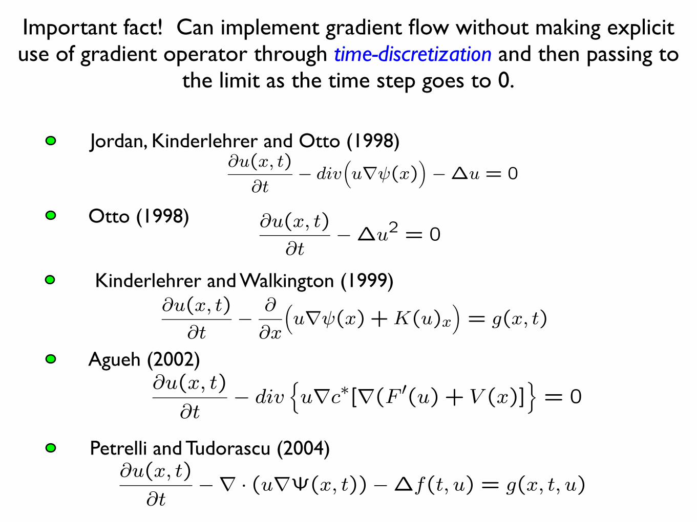
Important fact! Can implement gradient flow without making explicit use of gradient operator through time-discretization and then passing to

the limit as the time step goes to 0.

Jordan, Kinderlehrer and Otto (1998)

Otto (1998)

∂u(x, t)

∂t− ∆u2 = 0

Jordan, Kinderlehrer & Otto (1998)

∂u(x, t)

∂t− div

(u∇ψ(x)

)− ∆u = 0

Kinderlehrer & Walkington (1999)

∂u(x, t)

∂t−

∂

∂x

(u∇ψ(x) + K(u)x

)= g(x, t)

Agueh (2002)

∂u(x, t)

∂t− div

u∇c∗[∇(F ′(u) + V (x)]

= 0

Petrelli & Tudorascu (2004)

∂u(x, t)

∂t−∇ · (u∇Ψ(x, t))−∆f(t, u) = g(x, t, u)

4

Kinderlehrer and Walkington (1999)

Otto (1998)

∂u(x, t)

∂t− ∆u2 = 0

Jordan, Kinderlehrer & Otto (1998)

∂u(x, t)

∂t− div

(u∇ψ(x)

)− ∆u = 0

Kinderlehrer & Walkington (1999)

∂u(x, t)

∂t−

∂

∂x

(u∇ψ(x) + K(u)x

)= g(x, t)

Agueh (2002)

∂u(x, t)

∂t− div

u∇c∗[∇(F ′(u) + V (x)]

= 0

Petrelli & Tudorascu (2004)

∂u(x, t)

∂t−∇ · (u∇Ψ(x, t))−∆f(t, u) = g(x, t, u)

4

Agueh (2002)

Otto (1998)

∂u(x, t)

∂t− ∆u2 = 0

Jordan, Kinderlehrer & Otto (1998)

∂u(x, t)

∂t− div

(u∇ψ(x)

)− ∆u = 0

Kinderlehrer & Walkington (1999)

∂u(x, t)

∂t−

∂

∂x

(u∇ψ(x) + K(u)x

)= g(x, t)

Agueh (2002)

∂u(x, t)

∂t− div

u∇c∗[∇(F ′(u) + V (x)]

= 0

Petrelli & Tudorascu (2004)

∂u(x, t)

∂t−∇ · (u∇Ψ(x, t))−∆f(t, u) = g(x, t, u)

4

Petrelli and Tudorascu (2004)

Otto (1998)

∂u(x, t)

∂t− ∆u2 = 0

Jordan, Kinderlehrer & Otto (1998)

∂u(x, t)

∂t− div

(u∇ψ(x)

)− ∆u = 0

Kinderlehrer & Walkington (1999)

∂u(x, t)

∂t−

∂

∂x

(u∇ψ(x) + K(u)x

)= g(x, t)

Agueh (2002)

∂u(x, t)

∂t− div

u∇c∗[∇(F ′(u) + V (x)]

= 0

Petrelli & Tudorascu (2004)

∂u(x, t)

∂t−∇ · (u∇Ψ(x, t))−∆f(t, u) = g(x, t, u)

4

Otto (1998)Otto (1998)

∂u(x, t)

∂t− ∆u2 = 0

Jordan, Kinderlehrer & Otto (1998)

∂u(x, t)

∂t− div

(u∇ψ(x)

)− ∆u = 0

Kinderlehrer & Walkington (1999)

∂u(x, t)

∂t−

∂

∂x

(u∇ψ(x) + K(u)x

)= g(x, t)

Agueh (2002)

∂u(x, t)

∂t− div

u∇c∗[∇(F ′(u) + V (x)]

= 0

Petrelli & Tudorascu (2004)

∂u(x, t)

∂t−∇ · (u∇Ψ(x, t))−∆f(t, u) = g(x, t, u)

4

1. Set up variational principle

Time-discretized gradient flows

minu∈M

1

2hd

(uh

k−1, u)2

+ E(u)

(P )

Let h > 0 be the time step. Define the sequence recursively

solution of the minimization problemas follows: is the intial datum ; given , define as the

u

hk

k≥0

uhk

uhk−1u

h0 u

0

where d, the Wasserstein metric, is defined as

d(µ+, µ−)2 := infµ∈M

∫#d×#d

|x − y|2dµ(x, y)

i.e. d is the least cost of Monge-Kantorovich mass reallocation of to

for .

µ+

µ−

c(x, y) = |x − y|2

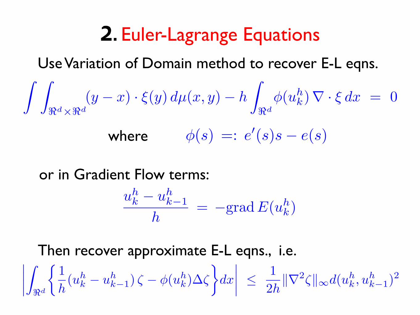
2. Euler-Lagrange Equations

∣∣∣∣∫!d

1

h(uh

k − uhk−1) ζ − φ(uh

k)∆ζ

dx

∣∣∣∣ ≤1

2h‖∇2ζ‖∞d(uh

k , uhk−1)

2

Then recover approximate E-L eqns., i.e.

Use Variation of Domain method to recover E-L eqns.

where φ(s) =: e′(s)s − e(s)

∫ ∫!d×!d

(y − x) · ξ(y) dµ(x, y) − h

∫!d

φ(uhk)∇ · ξ dx = 0

or in Gradient Flow terms:uh

k− uh

k−1

h= −gradE(uh

k)

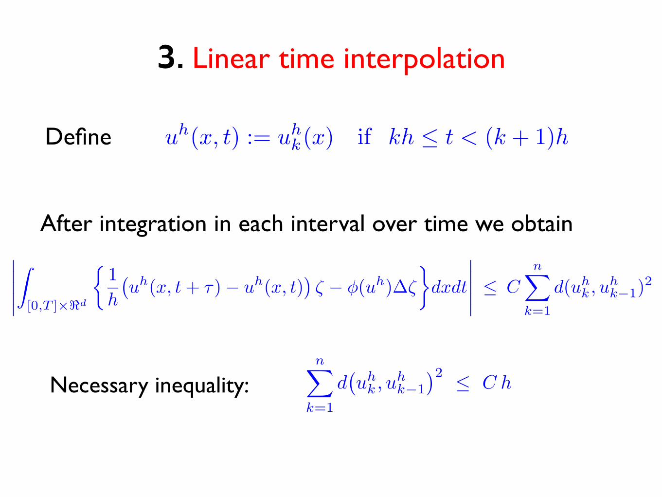
3. Linear time interpolation

∣∣∣∣∣∫

[0,T ]×"d

1

h

(uh(x, t + τ) − uh(x, t)

)ζ − φ(uh)∆ζ

dxdt

∣∣∣∣∣ ≤ C

n∑k=1

d(uhk , uh

k−1)2

After integration in each interval over time we obtain

Necessary inequality:n∑

k=1

d(uh

k , uhk−1

)2≤ C h

uh(x, t) := uhk(x) if kh ≤ t < (k + 1)hDefine

4. Convergence result as time step h goes to 0

Linear case Through a Dunford-Pettis like criteria show existence of function u such that, up to a subsequence, in some space.u

h u L

p

Then, passing to the limit in the general Euler-Lagrange equation shows that u is a “weak” solution of ∂u

∂t= ∇ ·

(u∇e′(u)

) (≡ ∆ φ(u)

)

Nonlinear case

L1

Stronger convergence is needed, through precompactness result in . Also needed discrete maximum principle:

u0

bounded ⇒ uh

bounded

Nonlinear Diffusion Problems

Theorem 4. Assume (f1)-(f3), (g1)-(g4) and (Ψ), then the problem (NP) admits a nonnegative essentially bounded weak solution provided that Ω is bounded and convex and the initial data is nonnegative and essentially bounded.u

0

ut −∇ · (u∇Ψ(x, t)) − ∆f(t, u) = g(x, t, u) in Ω × (0, T ),(u∇Ψ + ∇f(t, u)

)· νx = 0 on ∂Ω × (0, T ), (NP )

u(·, 0) = u0 ≥ 0 in Ω.

f(t, ·) differentiable,∂f

∂spositive and monotone in time (f3)

(u − v)(f(t, u) − f(t, v)) ≥ c|u − v|ω for all u, v ≥ 0, (f1)

f(·, s) are Lipschitz continuous for s in bounded sets (f2)

g(x, ·, ·) nonnegative in [0,∞) × [0,∞) for all x ∈ $d (g1)

g(x, t, u) ≤ C(1 + u) locally uniformly w.r.t. (x, t), t ≥ 0 (g2)

g(x, t, ·) is continuous on [0,∞) (g3)

g(x, ·, u)(x,u) is equicontinuous on [0,∞) w.r.t. (x, u) (g4)

Ψ : !d× [0,∞) → ! diff.ble and locally Lipschitz in x ∈ !

d (Ψ)

Hypothesis

Novelties

f(t, ·)Time-dependent potential and diffusion coefficientΨ(·, t)

Non homogeneous forcing term g(x, t, u)

Averaging in time for , and , e.g.Ψ f g Ψk :=1

h

∫ (k+1)h

kh

Ψ(·, t) dt

minu∈M

1

2hd

(vh

k−1, u)2

+ E(u)

(P ′)

New variational principle for vk−1 := uk−1 +

∫ kh

(k−1)hg(·, t, uk−1) dt

New discrete maximum principle

Lemma 5. If a.e. in Ω for large enough , then there exists such that a.e. in Ω, for all h > 0 if f satisfies (f3), uniformly in t > 0 and for s > 0 large enough we have

does not change sign for all t > 0, η > 1,

0 ≤ u0 ≤ M0 < ∞

M0 0 < M = M(M0) < ∞

0 ≤ uh ≤ M

lims↑∞

φs(t, s) = ∞

ηs∂f

∂s(t, ηs + η − 1) − (ηs + η − 1)

∂f

∂s(t, s)

∂f

∂s(·, s)being nonnegative if is increasing and

nonpositive if decreasing.

New discrete maximum principle

u0

bounded ⇒ uh

bounded

vhk−1 ≤ Uk := (φ′)

(−1) (Mk − Ψk) ⇒ uh

k ≤ Uk

Keyinequality:

where is the solution of the k-th “homogeneous stationary” equation, i.e.

Uk

−∇ · (u∇Ψk) − ∆fk(u) = 0

Signed measures

ut −∇ · (u∇Ψ(x, t)) − γ ∆u = g(x, t) in Ω × (0, T ),(u∇Ψ + γ ∇u

)· νx = 0 on ∂Ω × (0, T ), (SMP )

u(·, 0) = u0 in Ω.

Let and define

uh(x, t) := u(k)(x) for kh ≤ t < (k + 1)h

u(k)

:= uk+ − u

k−

where and

Let

gk±(x) :=

1

h

∫ h(k+1)

hk

g±(x, t) dtvk± := uk

± + h gk±

uk± := argmin

1

2d(u, vk−1

± )2 + hFk(u)

over all u ∈ M

vk−1

±

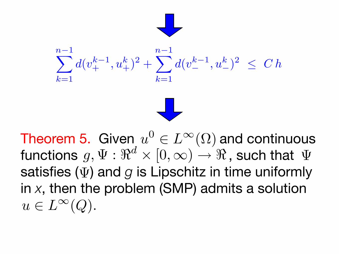
n−1∑

k=1

d(vk−1+ , uk

+)2 +n−1∑

k=1

d(vk−1−

, uk−

)2 ≤ C h

Theorem 5. Given and continuous functions , such that satisfies ( ) and g is Lipschitz in time uniformly in x, then the problem (SMP) admits a solution

u0∈ L

∞(Ω)g,Ψ : !d

× [0,∞) → ! Ψ

Ψ

u ∈ L∞(Q).

Why use gradient flows with Wasserstein metric?

We can minimize directly in the weak topologyWasserstein metric convergence is equivalent to weak star convergence

There are no derivatives in the variational principle this allows for use of discontinuous functions in approximation,

for example step functions

We can construct new (convex) variational principles for problems like the convection diffusion equation

We can recover new maximum principlesfairly easily from the variational principles