Prepared for submission to JHEP PDEs, ODEs, Analytic Continuation, Special Functions, Sturm-Liouville Problems and All That 1 C.P. Burgess Department of Physics, McGill University These notes present an introduction to mathematical physics, and in particular the solution of linear ordinary and partial differential equations that commonly arise in physics. Developed in Autumn 1990 for the course Physics 355A at McGill University. 1 ‘Primer on Partial Differential Equations for Physicists’, c 1990 Cliff Burgess
Transcript
Prepared for submission to JHEP
PDEs, ODEs, Analytic Continuation, Special Functions,
Sturm-Liouville Problems and All That1
C.P. Burgess Department of Physics, McGill University
These notes present an introduction to mathematical physics, and in particular the solution
of linear ordinary and partial differential equations that commonly arise in physics.
Developed in Autumn 1990 for the course Physics 355A at McGill University.
2 Partial Differential Equations of Mathematical Physics 5
2.1 Sample P.D.E.’s 5
2.2 A Typical Derivation 7
3 General Properties of Ordinary Differential Equations 11
3.1 Introduction 11
3.2 The Space of Solutions 11
3.3 The Wronskian 13
3.4 Initial-Value Problems 15
4 Boundary Value Problems 17
4.1 The Space of Solutions 17
4.2 Boundary-Value Problems 18
5 Separation of Variables 25
5.1 An Example and Some General Features 25
5.2 Cylindrical Coordinates 28
5.3 Spherical Polar Coordinates 30
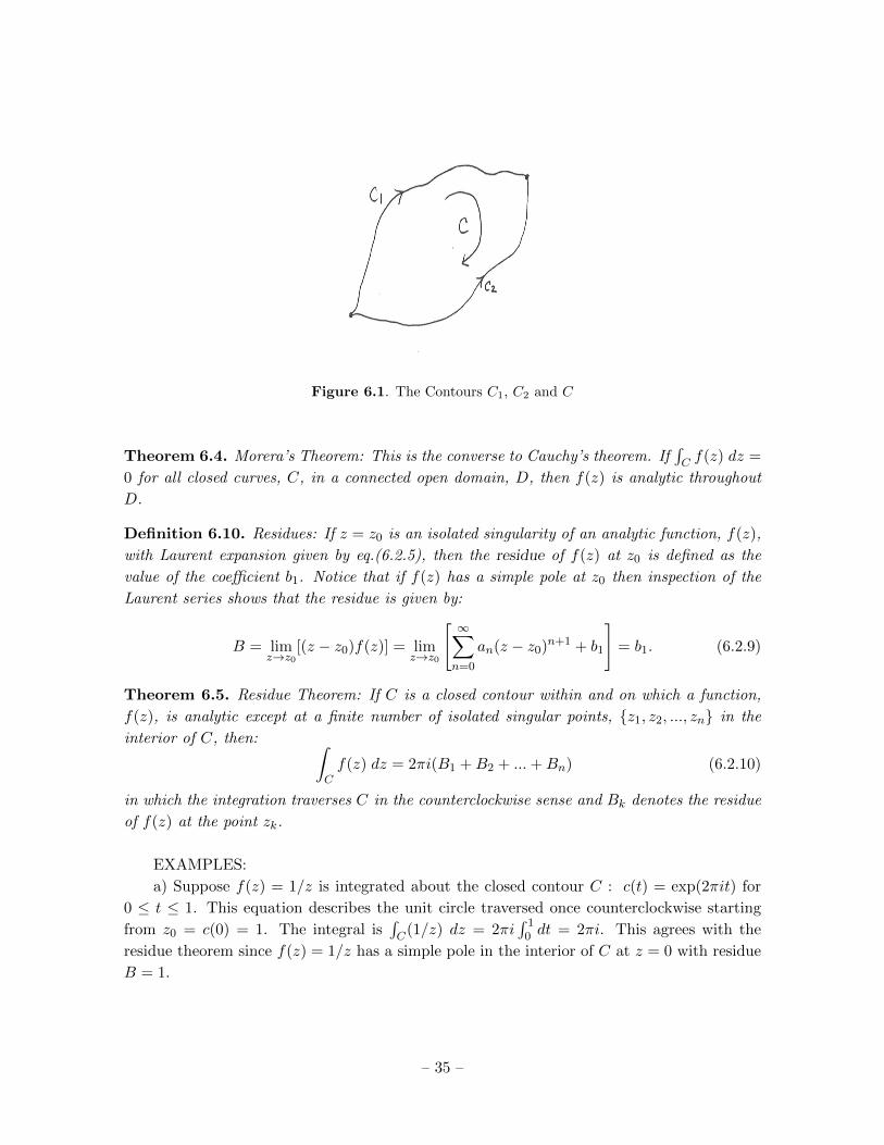
6 Complex Variables and Analytic Continuation 32
6.1 Introduction 32
6.2 Review of the Calculus of a single Complex Variable 32
6.3 Analytic Continuation: Uniqueness 37
6.4 Methods of Analytic Continuation 39
6.5 Euler’s Functions Gamma and Beta 41
7 Asymptotic Forms and the Method of Steepest Descent 47
7.1 The Approximation 47
7.2 The Accuracy of the Approximation 50
8 Power-Series Solutions 54
8.1 Introduction 54
8.2 Ordinary Points 54
8.3 Singular Points 59
8.4 Regular Singular Points 65
8.5 When the Method Fails: s2 − s1 = N 68
– i –
9 Classification of Ordinary Differential Equations 72
9.1 Introduction 72
9.2 The Hypergeometric Equation 73
9.3 The Confluent Hypergeometric Equation 78
9.4 Connection to Commonly Occuring Equations 78
10 Special Functions 82
10.1 Introduction 82
10.2 Hypergeometric Functions 82
10.3 Confluent Hypergeometric Functions 83
10.4 Integral Representations 87
10.5 Recurrence Relations 90
10.6 Legendre Functions 92
10.7 Bessel Functions 97
11 Sturm-Liouville Problems 105
11.1 Introduction 105
11.2 Some Linear Algebra 105
11.3 Infinite-Dimensional Generalizations 108
11.4 Self-Adjoint Operators 111
11.5 Examples 113
12 The Grand Synthesis 118
12.1 Example I: Laplace’s Equation 118
12.2 Example II: The Diffusion Equation 122
1 Overview
These notes are meant to provide an introduction to several very useful techniques of mathe-
matical physics, which are developed using as a vehicle the very common physical problem of
solving boundary-value problems for second-order linear partial differential equations (PDEs).
Along the way this requires the development of other very useful tools, including an explo-
ration of the properties of second-order linear ordinary differential equations (ODEs), and in
many cases the systematic construction of their solutions.
One of the main lines of development is the construction of series solutions, whose de-
scription provides an excuse for a lightning review of several other topics within the calculus
of complex variables, including the techniques of analytic continuation that allow the exten-
sion to more general domains of solutions initially developed in series form. In particular a
description is given of the theory of the kinds of singularities that are possible for solutions of
– 1 –
these ODEs, and how to find those solutions that have logarithmic singularities (and so are
at first sight not obtainable using series techniques).
The extension of solutions in this way, and the special functions to which this leads, are
presented in a more unified way than is often done. Rather than regarding each type of special
function on its own terms, with properties to be developed on a case-by-case basis, the notes
instead classify the kinds of differential equations that typically arise in physical applications.
In particular, since these usually lead to equations involving three (or fewer) regular-singular
points (RSPs, whose precise definition is given when appropriate below), the most general
form of this equation is identified and solved once and for all. Since the most general ODE
of this type is the Hypergeometric equation, the properties of the solutions to this equation
— Hypergeometric functions — are studied in some detail. It is because so many physical
systems involve equations with three or fewer RSPs that most of the special functions usually
studied are special cases of these Hypergeometric functions, and this is why their properties
follow as special cases of those of the Hypergeometric functions.
Also discussed in detail are the Confluent Hypergeometric equations and functions, that
are obtained when two of the RSPs happen to coalesce to give an ODE with one regular and
one irregular singular point. The properties of these functions (and their many special cases
of physical interest, such as Bessel functions) are also obtained as limiting instances of the
general Hypergeometric case.
The main bridge from solutions to ODEs to solutions of PDEs comes through the tech-
nique of separation of variables, which constructs solutions in product form — such as
ψ(x, y) = X(x)Y (y). Of course most solutions to PDEs do not have this form, so the key
idea is that a general solution to the PDE can be written as a linear combination of solutions
in this product form. This leads to the discussion of Sturm-Liouville problems and the use
of special functions as bases for the expansion of more general functions — including Fourier
series, Fourier-Bessel series and so on. This brings out the relationship between calculus
and linear algebra, in a way that connects the treatments of classical electrodynamics and
quantum mechanics that undergraduates usually study at the same time as mathematical
physics.
These are old subjects that at one time were part of the standard lore for physicists, but
some of them are less often taught nowadays due to the advent of cheap numerical methods.
Although such numerical methods are of course very useful (and should always be exploited),
it behooves the well-trained physicist also to know these more analytic methods. They are
useful both to understand how the numerical methods work, but also to allow one to check
one’s numerics by providing analytic comparisons in various limits.
A Road Map
The presentation of the remainder of the notes proceeds as follows. The first few sections
describe the types of linear second-order PDEs that often arise in physics, and argue why it
is that the types of equations encountered are often so similar in physical applications. The
procedure of separation of variables is then described in a few simple examples.
– 2 –
There follows then a lengthy discussion about constructing solutions to linear second-
order ODEs. This involves first describing general properties of the vector space of their
solutions, and then moves on to the discussion of the construction of series solutions as well
as of the limitations of this procedure. Along the way is a telegraphic summary of some useful
results in the calculus of a single complex variable, including contour integration and analytic
continuation, since these are often missing in the background of an undergraduate learning
this material.
Next comes the classification of the ODEs arising in physical applications, and the demon-
stration that most problems encountered fall into the class described by Hypergeometric func-
tions. The properties of these are then enumerated, followed by a discussion of how the usual
special functions (Bessel, Legendre, Gegenbauer, Hermite, Laguerre, etc) arise as special cases
of the Hypergeometric functions.
The penultimate sections explore how the space of solutions to a linear PDE is a vector
space and how separated solutions involving the above the special functions can be used to find
a basis of this vector space, the bailiwick of Sturm-Liouville problems. All these techniques
are tied together in the final section which uses them to solve several explicit example PDE
examples from start to finish.
1.1 Introduction
Consider a physical variable, ψ(x, y, z, t), that varies throughout space, (x, y, z), and time,
t. ψ could represent the pressure, density or temperature of a fluid, or the value of the
electromagnetic scalar potential, or any number of other continuous physical variables. The
evolution of such an object in time is generally described by a partial differential equation,
or P.D.E.. These equations are the analogue for a continuously varying variable of the usual
ordinary differential equations describing the motion of a particle. For instance Newton’s
laws for the motion of an element of fluid might take the form:
∂2ψ
∂t2+ F
[ψ,∂ψ
∂t,∇ψ, ...
]= 0. (1.1.1)
in which F gives the ‘force’ acting on ψ at every point as a function of the behaviour of ψ in
the neighbourhood of that point. Different physical situations will be described by different
functional forms for F .
From a mathematical point of view, a physicist’s role in life is to find which P.D.E.’s
describe which physical problems (i.e. which functions, F ) and then to construct and interpret
the corresponding solutions. For this reason a great deal of effort in theoretical physics and
applied mathematics is and has been devoted to the solving of these differential equations.
F can be some horribly complicated function of its arguments, and in this general case
only very little may be said about the properties of the solutions to eq. (1.1.1). A problem
that is much better understood, and which nevertheless has applications to many physical
situations, is the case where ψ and its derivatives are in some sense ‘small’. In this case one
– 3 –
can imagine expanding F in powers of its arguments as follows:
F
[ψ,∂ψ
∂t,∇ψ, ...
]≈ −f + Cψ +
4∑i=1
Bi∂ψ
∂xi+
4∑i=1
4∑j=1
Aij∂2ψ
∂xi∂xj+ · · · . (1.1.2)
The coefficient functions f , C, Bi and Aij may all depend on the coordinates x, y, z and t.
The ellipsis (i.e. ‘· · · ’) denote terms involving higher derivatives and/or higher powers of ψ
and its derivatives. These may be neglected when ψ and its derivatives are sufficiently small.
Neglecting these terms and using eq. (1.1.2) in the P.D.E. (1.1.1) gives a differential
equation that is linear in ψ and at most second order in its derivatives. A good deal more is
known about the construction of solutions to these problems.
These lectures are devoted to solving the linear, second-order P.D.E.’s that arise most
frequently in mathematical physics. Having said this, less than half of the course (chapters 4,
5 and 12) is actually spent directly solving these P.D.E.’s. The remaining chapters (6 through
11) are devoted to a long digression on generating solutions to the linear second-order ordinary
differential equations (O.D.E.’s) and to describing their solutions in some detail.
A major reason for this digression is that much of the theory of P.D.E.’s can be con-
structed by using the corresponding theory of O.D.E.’s as a guide. This line of argument is
fleshed out in Chapters 3 and 4.
Furthermore, the principal method of solution discussed here for P.D.E.’s is the method
of Separation of Variables (Chapter 5) in which the partial differential problem is reduced
to the construction of solutions to a related set of O.D.E.’s. This technique consists of the
construction of solutions with a specific dependence upon the independent variables x, y, z
and t:
ψ(x, y, z, t) = X(x)Y (y)Z(z)T (t). (1.1.3)
This would superficially appear to have limited utility since the solution to a generic
physical problem does not have this separated form. The key observation is then that although
the general solution does not have this separated form it is often possible to find a basis of
solutions with this form. Any solution may then be written as a linear combination of this
basis of solutions. The construction of this basis is performed in Chapters 8 through 10 and
the claim that any solution may be expanded in terms of the basis is the topic of Chapter 11.
Chapter 12 is then a summary in which all of the parts of the argument are pulled together
and applied to specific boundary-value problems.
A completely different reason for the lengthy detour through the theory of O.D.E.’s is that
many of these topics, such as Analytic Continuation and Steepest Descent (Chapters 6 and
7), Special Functions (Chapters 9 and 10), and Self-Adjoint Eigenvalue Problems (Chapter
11), are useful in their own right elsewhere in mathematical physics. The problem of solving
the P.D.E.’s is being partially used here as the vehicle through which they are presented.
– 4 –
2 Partial Differential Equations of Mathematical Physics
Our goal is to find solutions to the 2nd order, linear P.D.E.’s that arise in mathematical
physics. This section first describes the P.D.E.’s that commonly arise in physical problems
and then gives an illustrative derivation of one such P.D.E.. Some arguments are presented
as to why the P.D.E.’s of interest take the form that they do.
2.1 Sample P.D.E.’s
The most general 2nd order, linear, inhomogeneous P.D.E. governing a variable, ψ, that
depends on the coordinates xk, k = 1, .., 4 with x1 = x, x2 = y, x3 = z, and x4 = t, is:
Lψ = f.
Here f = f(xk) is a known function of the coordinates, xk, and L is the following differential
operator:
Lψ =
4∑i=1
4∑j=1
Aij(xk)∂2ψ
∂xi∂xj+
4∑i=1
Bi(xk)∂ψ
∂xi+ C(xk)ψ (2.1.1)
The coefficients, Aij , Bi, and C are, like f , all given functions of the coordinates only and
not of ψ itself. It is conventional to choose Aij to be symmetric Aij = Aji, as may always be
done without loss of generality.
Solutions of the general P.D.E. are not known so it is fortunate that the most general
form given by eq.(2.1.1) does not often (if ever) arise in mathematical physics. Those P.D.E.’s
that do arise most frequently are listed below:
1. Laplace’s Equation:
Many time-independent problems, such as the description of an electrostatic potential
in the absence of charges, are described by Laplace’s equation. This is defined for
ψ = ψ(x, y, z) by:
∇2ψ =∂2ψ
∂x2+∂2ψ
∂y2+∂2ψ
∂z2= 0. (2.1.2)
The differential operator, ∇2, defined by eq.(2.1.2) is called the Laplacian operator, or
just the Laplacian for short.
2. Poisson’s Equation:
The inhomogeneous version of Laplace’s equation is called Poisson’s equation. It governs
the behaviour of an electrostatic potential in the presence of charge distributions, for
example. It has the form:
∇2ψ = f(x, y, z) (2.1.3)
in which f is a known function.
– 5 –
3. Helmholtz’s Equation:
The equation:
∇2ψ + k2ψ = 0 (2.1.4)
is known as Helmholtz’s equation. k is a constant. This equation arises in, among other
places, the study of the propagation of waves.
4. Schrodinger’s Equation:
A great deal of quantum mechanics is devoted to the study of the solutions to the
time-dependent Schrodinger equation:
− ~2
2m∇2ψ + V (x, y, z)ψ = i~
∂ψ
∂t. (2.1.5)
This equation governs the time dependence of the wave-function of a particle moving in
a given potential, V (x, y, z). A special role is played by solutions to (2.1.5) that have the
simple form: ψ = φ(x, y, z) exp(−iEt/~). The function φ satisfies the time-independent
Schrodinger equation:
− ~2
2m∇2φ+ V (x, y, z)φ = Eφ. (2.1.6)
In both of these equations ~, m, and E represent real constants. i, as usual, satisfies
i2 = −1.
5. The Diffusion Equation:
The P.D.E. governing the diffusion of a quantity, such as the number of particles per
unit volume present in a region, is the diffusion equation:
∂ψ
∂t− κ∇2ψ = 0. (2.1.7)
κ = k2 denotes here a real constant.
6. The Wave Equation:
Wave propagation, including pressure waves in fluids, electromagnetic waves and grav-
itational waves all satisfy the following wave equation:
− 1
v2
∂2ψ
∂t2+∇2ψ = 0. (2.1.8)
The real constant v can be interpreted as the speed of the corresponding wave.
7. The Klein-Gordon Equation:
Disturbances travelling through fields that mediate forces with a finite range, satisfy a
modification of the wave equation called the Klein-Gordon equation. It is given by:
− 1
c2
∂2ψ
∂t2+∇2ψ +
m2c2
~2ψ = 0. (2.1.9)
The coefficients c, ~ and m all represent constants.
– 6 –
There are several features that these P.D.E.’s have in common:
1. The techniques used to solve these equations rely on a property that they all share.
This common property is the feature that they are all linear in the dependent variable,
ψ. Although the theory of linear equations has received the bulk of attention from
applied mathematicians and theoretical physicists, it is by no means true that most
of the P.D.E.’s that arise in real physical problems are linear. The prominence of
linear equations in this list reflects the fact that these equations can be generally solved
whereas comparable methods of solution for nonlinear equations are relatively scarce.
In some physical situations, however, linear equations provide an adequate approxima-
tion to a nonlinear problem. Nonlinear terms in a differential equation are those that
involve quadratic and higher powers of the field, ψ, or its derivatives. If ψ and its
derivatives are small enough then its square and higher powers may be expected to be
smaller still. In this case any linear terms in a P.D.E. may be expected to dominate
the nonlinear ones. Besides the advantage of being well understood, linear P.D.E.’s are
therefore also of interest as an approximation to the full nonlinear behaviour in the
limit of weak, slowly varying fields.
2. As pointed out in the introduction, these P.D.E.’s all involve at most two derivatives
with respect to the independent variables, x, y, z and t. This usually arises from the
physical requirement of stability since equations involving higher time derivatives gener-
ically admit runaway solutions. In some cases the physics of interest does lead to
equations involving higher than second derivatives. In these cases the neglect of the
higher-derivative terms is justified by the approximation that the fields in the problem
are slowly varying in space and time.
3. All of the above equations have two more features in common. Firstly, there are ab-
solutely no terms that involve just a single spatial derivative. Secondly, the second
derivative of ψ with respect to the spatial coordinates always appears in the combina-
tion∇2ψ. This is a reflection of the underlying symmetry of the corresponding problems
with respect to spatial rotations. A similar observation holds for the combination of
derivatives that appears in the wave equation and in the Klein-Gordon equation. These
can be derived by requiring that they be invariant with respect to the Lorentz transfor-
mations of special relativity.
4. With the exception of the two Schrodinger equations all of the homogeneous P.D.E.’s
listed involve only constant coefficients. This follows from the invariance of the under-
lying physical situations under translations in space and time.
2.2 A Typical Derivation
It is useful to have in mind some idea of how these equations arise in physical situations
because physical intuition about the underlying problem is a useful guide when trying to
– 7 –
derive the properties of their solutions. We therefore now turn to a simple derivation of one
of the above equations. We take the diffusion equation as our example.
Consider a system contained within some volume, R, consisting of an ideal gas that is lo-
cally in thermal equilibrium. Local equilibrium means that each small volume element of the
medium is assumed to be in equilibrium with its immediate surroundings, allowing thermo-
dynamic variables such as temperature, T (x, y, z, t), and energy per unit volume, U(x, y, z, t),
to be defined at each point. For an ideal gas these are related by: U = cvT in which cv is
the specific heat at constant volume and is independent of x, y, z and t. Thermodynamic
stability requires that cv be positive. We wish to understand how an initially inhomogeneous
temperature distribution will diffuse throughout R.
Consider an arbitrary volume, V , contained within R. The first law of thermodynamics
relates the rate of change of the energy contained within V to the rate of heat flow (i.e. heat
flux) into V . Denoting the energy within V as
E =
∫VU dV =
∫VcvT dV, (2.2.1)
the first law states:dE
dt=δQ
δt. (2.2.2)
δQ/δt denotes the total heat flux into V . In this system heat moves about as a result of the
motion of the gas molecules. The heat flux per unit time through any surface element, n dS,
can be described in terms of a heat-flux vector: q(x, y, z, t), defined throughout R. Here
n(x, y, z) denotes the unit normal to the surface element and dS is its infinitesimal area. The
flux through the surface element is given in terms of q by q · n dS.
The heat flux into V is then given by:
δQ
δt= −
∫∂V
q · n dS (2.2.3)
in which ∂V denotes the boundary of V and n is the outward-pointing unit normal to the
boundary. Combining eqs.(2.2.2) and (2.2.3) allows the first law to be written:
cv
∫V
∂T
∂tdV = −
∫∂V
q · n dS. (2.2.4)
Using the divergence theorem: ∫∂V
q · n dS =
∫V∇ · q dV (2.2.5)
then gives: ∫V
(cv∂T
∂t+∇ · q
)dV = 0, for all V ⊂ R. (2.2.6)
Since the integral over V in eq.(2.2.6) must vanish for any choice of V that lies within R, it
must be true that the integrand itself vanishes throughout R if it is sufficiently smooth. To
– 8 –
see this argue as follows: We know that∫V f dV = 0 for all V ⊂ R and we wish to argue
that f(p) = 0 for any p ∈ R. The argument proceeds by contradiction. Assume therefore
that f(p) is not zero for some p ∈ R. f(p) must then be either positive or negative. If
f(p) > 0 then, if f is continuous, f must also be positive throughout some neighbourhood,
N , containing p. Choose, then, V ⊂ N ⊂ R so that f is positive throughout the entire region
of integration. Since the integral of a positive function is itself positive it must be that, for
this V ,∫V f dV > 0 in contradiction with the assumption that this integral vanishes. The
argument is identical if f(p) is instead assumed to be negative. This lemma therefore allows
us to conclude from eq.(2.2.6) that:
cv∂T
∂t+∇ · q = 0 (2.2.7)
throughout R. This is the local expression of the physical content of the first law: conservation
of energy.
In order to proceed further we need another piece of information that relates T to q.
This is provided by a phenomenological relation of the form:
q = q[T,∇T, ...]. (2.2.8)
This expresses how the transport of energy is governed by the properties of the surrounding
gas. It could in principle be derived from the equations of motion of the underlying gas
molecules. If, however, T is assumed to be varying slowly throughout space we expect that
q should be well approximated by those terms that involve the fewest derivatives of T . Since
q is a vector quantity so must be the right-hand-side of eq.(2.2.8). There is only one term
possible that both transforms like a vector and involves the fewest number of derivatives of
T and this is:
q ≈ −λ2∇T. (2.2.9)
The sign of the right-hand-side of eq.(2.2.9) is chosen so that q points in the direction of de-
creasing temperature, as would be expected physically. The real constant λ can be calculated
in principle from an understanding of the motion of the underlying molecules.
Equations (2.2.7) and (2.2.9) may now be used to elimate q and so derive an equation
involving just T . Taking the divergence of eq.(2.2.9), and using the identity ∇ · ∇T = ∇2T ,
gives the diffusion equation:∂T
∂t− κ∇2T = 0. (2.2.10)
The diffusion constant, κ, is found to be related to λ and cv by κ = λ2/cv. This is a manifestly
positive quantity.
The diffusion equation has many solutions. Being a linear homogeneous equation indeed
implies that the sum of any two solutions is itself a solution. The real temperature distribution
occuring in any physical problem, however, satisfies both the diffusion equation and a set of
boundary conditions. The above derivation gives some physical intuition for what kinds of
– 9 –
conditions would be necessary to specify the solution uniquely—that is to say, what constitutes
a well-posed boundary-value problem for the diffusion equation.
Physically, the behaviour of the temperature in R should depend on both the initial tem-
perature distribution and the amount of heat flux, if any, that passes through the boundary,
∂R, of R. We expect, therefore, that a well-posed boundary-value problem for the diffusion
equation would be to find the temperature distribution, T (x, y, z, t), satisfying:
∂T
∂t= κ∇2T for all (x, y, z) ∈ R and for all t
and: T = τ(x, y, z) for all (x, y, z) ∈ R and for t = 0
and: n · ∇T = f(x, y, z, t) for all (x, y, z) ∈ ∂R and for all t
We prove in the following sections that these conditions do indeed guarantee a unique
solution to this equation.
– 10 –
3 General Properties of Ordinary Differential Equations
3.1 Introduction
Our goal is to construct solutions to P.D.E.’s such as those listed in the previous section. In
order to do so we must answer the following general questions:
1. What is the general solution?
2. What constitutes a well-posed boundary-value problem?
3. How is the general solution constructed?
4. Given the general solution, what is the particular solution satisfying a given set of
boundary conditions?
Our strategy in answering these questions is to use experience with ordinary differential
equations, O.D.E.’s, as a guide. The method used to construct the solutions of the P.D.E.’s
also consists of reducing the problem to one of solving an equivalent set of O.D.E.’s. This
chapter is therefore devoted to a review of the answer to the analoguous problems in the
theory of linear 2nd-order O.D.E.’s. The explicit construction of, and a discussion of the
resulting properties of, their solutions is deferred to later chapters.
3.2 The Space of Solutions
The general form for a linear, 2nd-order O.D.E. is:
a(x)y′′ + b(x)y′ + c(x)y = g(x). (3.2.1)
where a, b, c and g are given real functions of the real independent variable, x, and a vanishes
only at isolated points in the interval in which x takes its values. (If a were to vanish on some
interval the problem to be solved in this interval would be a first-order O.D.E. rather than a
second-order one.) It is conventional to divide the equation through by a(x) giving:
Ly = f(x)
with: Ly = y′′ + p(x)y′ + q(x)y. (3.2.2)
The new coefficient functions are related to the previous ones in an obvious way.
The fundamental property that underlies the approach to solving this O.D.E. is the
linearity of the differential operator L. By definition linearity is the statement that if y1(x)
and y2(x) are any two functions and α and β are real (or complex) numbers, then:
L(αy1 + βy2) = αLy1 + βLy2. (3.2.3)
The utility of this property follows from its wide-ranging consequences for the space of solu-
tions to these O.D.E.’s:
– 11 –
1. If y1 and y2 are both solutions to the O.D.E. Ly = f , with L given in eq.(3.2.2), then
yh = y2 − y1 satisfies the homogeneous equation:
L yh = 0. (3.2.4)
This implies that an arbitrary solution, y2, to (3.2.2) is given by any particular solution,
y1, plus a solution to the homogeneous equation, (3.2.4). The problem of finding the
general solution to the inhomogeneous equation is therefore reduced to the much simpler
problem of finding a single particular solution together with the problem of finding the
general solution to the homogeneous equation. We return to the construction of partic-
ular solutions to the inhomogeneous equation in chapter 13. Properties of solutions to
the homogeneous problem are the subject of the rest of this section.
2. Linearity also ensures that the space of solutions, S, to the homogeneous O.D.E., (3.2.4),
defined on some real interval [a, b], forms a vector space. That is, S together with the
two operations defined by:
pointwise addition: [y1 + y2](x) ≡ y1(x) + y2(x)
scalar multiplication: [αy](x) ≡ α[y(x)]
forms a vector space. The ‘zero vector’ of this vector space is the function that vanishes
for all x in [a, b].
The proof that these definitions of ‘vector addition’ and ‘scalar multiplication’ give Sa vector-space structure consists of a straightforward check of the defining properties
of a vector space. (See, for example, Topics in Algebra (Wiley).) Satisfaction of these
properties relies crucially, of course, on the linearity of L.
The significance of this fact is that it should therefore be possible to write any of the
elements of S, y say, as a linear combination of a basis of solutions. y(x) =∑
k ckyk(x)
with the ck’s being constants. The general solution to Ly = 0 is then known once a
basis of solutions is constructed.
In order to sharpen this logic recall the following definitions.
Definition 3.1. A set of vectors, {y1, ..., yn}, is linearly independent if and only if the equa-
tion c1y1 + ... + cnyn = 0 implies that all of the constants, {c1, ..., cn}, must vanish. The
set, {y1, ..., yn}, is said to be linearly dependent if it is not linearly independent. This is
equivalent to the existence of a set of constants, {c1, ..., cn}, not all vanishing, for which
c1y1 + ...+ cnyn = 0.
Definition 3.2. A vector space has dimension n if and only if both of the following are true:
(i) a set of n linearly independent vectors exists, and (ii) any set of n+ 1 vectors is linearly
dependent.
– 12 –
Definition 3.3. A basis of an n-dimensional vector space is any set of n linearly-independent
vectors.
Clearly these definitions imply that if {y1, ..., yn} forms a basis, then any other vector,
y, can be written as the sum y =∑
k ckyk. This follows from the fact that the n+ 1 vectors,
{y1, ..., yn, y}, must be linearly dependent. In the event that the vector space should prove to
be infinite dimensional a basis can be defined by this last condition that an arbitrary vector
can be expressed as a linear combination of basis vectors.
In practice, for the space of solutions, S, of Ly = 0 we need to answer the following
questions:
1. What is the dimension of S?
2. What constitutes a basis for S?
3. What kind of boundary conditions uniquely specify an element of S?
The remainder of this section is devoted to (partially) answering the problems in this
list. We first show that if any nonzero solution exists, then S is two-dimensional. We then
demonstrate how to construct from any nonzero solution a second linearly independent solu-
tion. These two elements of S form a basis. We finally show that the initial-value problem
is well posed, and so uniquely specifies a solution to the O.D.E.. The existence and explicit
construction of the first nonzero solution that these results assume is addressed in chapter 8.
3.3 The Wronskian
Before proceeding to the three results listed in the previous section a detour is necessary to
derive a more useful criterion for the linear independence of n functions. Recall that the
definition of linear independence, when applied to the solution space, S, is the following
statement:
c1y1(x) + ...+ cnyn(x) = 0 for all x =⇒ c1 = c2 = ... = cn = 0. (3.3.1)
Since the left-hand-side of this implication is true for all x it may be differentiated. Successive
differentiation shows that (3.3.1) is equivalent to:
c1y1(x) + ...+ cnyn(x) = 0
c1y′1(x) + ...+ cny
′n(x) = 0
...
c1y(n−1)1 (x) + ...+ cny
(n−1)n (x) = 0
for all x =⇒ c1 = c2 = ... = cn = 0. (3.3.2)
The left-hand-side has the form of a set of n linear equations in the n unknowns {c1, ..., cn}.Such a system of equations has c1 = c2 = ... = cn = 0 as its only solution if and only if the
– 13 –
following determinant does not vanish:
Wn(x) ≡
∣∣∣∣∣∣∣∣∣∣y1(x) . . . yn(x)
y′1(x) . . . y′n(x)...
. . ....
y(n−1)1 (x) . . . y
(n−1)n (x)
∣∣∣∣∣∣∣∣∣∣. (3.3.3)
This last equation defines the Wronskian of the n functions {y1(x), ..., yn(x)}. In terms of
Wn(x), the functions {y1(x), ..., yn(x)} are linearly independent if and only if there exists a
point, x0 ∈ [a, b], for which Wn(x0) 6= 0. Conversely, the {yk(x)} are linearly dependent if
and only if Wn(x) = 0 for all x ∈ [a, b].
With this test for linear dependence in hand we now turn to the discussion of S.
Theorem 3.1. Any three solutions, y1(x), y2(x) and y3(x), of the differential equation Ly =
0, with L given by eq.(3.2.2) are linearly dependent.
Proof. To prove this theorem consider the Wronskian:
W3(x) =
∣∣∣∣∣∣∣y1 y2 y3
y′1 y′2 y′3
y′′1 y′′2 y′′3
∣∣∣∣∣∣∣ . (3.3.4)
The differential equation (3.2.4) implies that y′′k + p(x)y′k + q(x)yk = 0 for k = 1, 2 and 3.
This implies that the bottom row of the matrix in eq.(3.3.4) is a linear combination of the
first two rows. Its determinant, W3(x), must therefore vanish for all x, as may be checked by
explicit evaluation. The three functions are therefore linearly dependent as claimed.
This theorem tells us that the space of solutions to the O.D.E. (3.2.4) is at most two-
dimensional. We now show that if S has any nonzero element at all, then it is exactly
two-dimensional.
Theorem 3.2. If y1(x) 6≡ 0 is a solution to the O.D.E. (3.2.4): Ly1 = 0, then a linearly-
independent solution, y2(x) exists. (The construction of the original solution, y1(x), is de-
ferred to a later section.)
Proof. This theorem is proven by explicitly constructing the second solution. Consider the
Wronskian of any two solutions to the O.D.E. (3.2.4):
W2(x) =
∣∣∣∣∣ y1 y2
y′1 y′2
∣∣∣∣∣ = y1y′2 − y2y
′1. (3.3.5)
Eq.(3.2.4) implies that W2(x) satisfies its own differential equation:
dW2
dx= y1y
′′2 − y2y
′′1 = −p(x)[y1y
′2 − y2y
′1] = −p(x)W2(x). (3.3.6)
– 14 –
This is easily integrated to yield the solution:
W2(x) = W2(x0) exp
(−∫ x
x0
p(u) du
). (3.3.7)
This last equation implies that once W2 is known at a single point, its value is determined
at all other points solely by the O.D.E.. The idea is to now regard eq.(3.3.5) as being an
equation from which y2 is to be determined in terms of a known function y1 and W2 given by
eq.(3.3.7). To solve rewrite eq.(3.3.5):
y21
d
dx
(y2
y1
)= W2(x) = A exp
(−∫ x
x0
p(u) du
),
divide by y21, and integrate:
y2(x) = y1(x)
[B +A
∫ x
du1
y21(u)
exp
(−∫ u
dv p(v)
)]. (3.3.8)
It is easily checked that y2(x) as defined by eq.(3.3.8) satisfies the O.D.E. (3.2.4) and
has a Wronskian with y1(x) given by W2 = A exp(−∫ x
p(u) du). Given any solution to
eq.(3.2.4), then, eq.(3.3.8) defines a second linearly independent solution provided only that
the integrals in eq.(3.3.8) converge. This is the result that was to be proven.
Given the existence of any nontrivial solution to the O.D.E. the last two theorems imply
that the space, S, of solutions is two-dimensional. Any nonzero solution, y1, together with
the second solution, y2, defined by eq. (3.3.8) gives a basis for S. This in turn implies that
the general solution to (3.2.4), yh(x) can be written in terms of these two basis solutions by
yh(x) = c1y1(x) + c2y2(x). The problem of finding the general solution to the O.D.E. (3.2.4)
has, in principle, boiled down to the construction of a single nonzero solution. As discussed
earlier, construction of such a solution also gives the general solution to the inhomogeneous
equation, eq. (3.2.2), when combined with any particular integral of that equation.
3.4 Initial-Value Problems
Since the general solutions of (3.2.2) and (3.2.4) involve two free constants, c1 and c2, we
expect to require two pieces of boundary information in order to get a unique solution. It
is important to realize, however, that just any two pieces of information need not make the
solution unique. Consider, for example, the following O.D.E. and boundary-value problem:
d2y
dx2+ y = 0 for x ∈ [0, π]
with: y(0) = y(π) = 0.
This problem has the one-parameter family of solutions: y(x) = a sinx.
There is a general lesson here. The reason this choice of boundary conditions proved
insufficient to determine the solution was that it, like the O.D.E. itself, was linear and ho-
mogeneous. That is, any linear combination of solutions to the O.D.E. and the boundary
– 15 –
conditions is also a solution of both. This implies that if any nonzero solution, y(x), exists
then so does the one-parameter family αy(x) for any real constant α.
Theorem 3.3. One choice of boundary conditions that is always guaranteed to give a unique
result for the O.D.E. (3.2.4) is the initial-value problem:
y(x0) = u anddy
dx(x0) = v (3.4.1)
with u and v not both zero.
Proof. To see that the solution to (3.2.2) with initial condition (3.4.1) is unique suppose
that two solutions, y1 and y2 exist. Their Wronskian is given by eq.(3.3.7) with W2(x0) =
y1(x0)y′2(x0) − y2(x0)y′1(x0) which vanishes by virtue of eq.(3.4.1). This implies that there
are two constants, c1 and c2 not both zero, for which c1y1(x) = c2y2(x) for all x ∈ [a, b].
Evaluating this equation at x = x0 then implies c1 = c2 6= 0 unless u vanishes. If u = 0 then
v cannot vanish so the argument may be repeated using c1y′1(x) = c2y
′2(x).
The case u = v = 0 is trickier since in this case the O.D.E. and boundary conditions are
both linear and homogeneous. Whether or not the initial-value problem is well-posed depends
in this case on how smooth the solutions are required to be. If the solutions are required to
be analytic on [a, b] then the solution is unique (and is identically zero). To see this notice
that y(x0) = y′(x0) = 0 together with the O.D.E. (3.2.4) implies that y′′(x0) = 0. Similarly,
repeated differentiation of the O.D.E. shows that all derivatives of y vanish when evaluated
at x0. This implies that every term in the Taylor expansion of y about x = x0 vanishes (see
section 6.2), so y = 0 throughout the interval [a, b]. The zero function is therefore the unique
analytic solution to the initial-value problem.
If, on the other hand, the solution to (3.2.4) with y(x0) = y′(x0) = 0 need not be analytic
then it need not be unique. To see this consider the following sample O.D.E.:
d2y
dx2− 1
x2
dy
dx+
2
x3y = 0 for x ∈ [0,∞).
A one-parameter family of solutions to this equation and the initial conditions y(0) = y′(0) = 0
is given by y = a exp(−1/x). Although y(x) is here infinitely differentiable it is not analytic
at x = 0.
Putting aside the properties of O.D.E.’s, we turn now to a consideration of the analogous
properties of the solutions to linear second-order P.D.E.’s.
– 16 –
4 Boundary Value Problems
4.1 The Space of Solutions
In the last chapter we established for linear second-order O.D.E.’s that:
1. The general solution to the inhomogeneous problem is given by a particular solution
plus the general solution to the homogeneous equation.
2. The space of solutions to the homogeneous equation forms a two-dimensional vector
space.
3. The initial-value problem in which the value of y and y′ are both specified, and do not
both vanish, at a given point, x0, guarantees a unique solution.
This section is devoted to exploring the same questions for solutions to P.D.E.’s.
The general linear second-order P.D.E. is given by
Lψ = f (4.1.1)
in which f is a known function of the independent variables, x, y, z and t, and the differential
operator, L, is given by eq.(2.1.1). The crucial property that this operator shares with
eq.(3.2.2) is the linearity, (3.2.3), of L. Just as was the case for the O.D.E., this ensures
that the difference, ψh = ψ2 − ψ1, between any two solutions to eq. (4.1.1) satisfies the
homogeneous equation
L ψh = 0. (4.1.2)
The strategy for finding the general solution to (4.1.1) is the same as for the corresponding
O.D.E.. It suffices to find the general solution to the homogeneous problem, (4.1.2), together
with any particular solution to (4.1.1).
The linearity of L as defined by eq.(2.1.1) guarantees that the set of solutions to the homo-
geneous equation, (4.1.2), forms a vector space. Addition of vectors and scalar multiplication
is defined pointwise: [ψ1 + ψ2](x, y, z, t) = ψ1(x, y, z, t) + ψ2(x, y, z, t) and [αψ](x, y, z, t) =
α[ψ(x, y, z, t)]. We again therefore expect to be able to write the general solution to (4.1.2)
as a linear combination of a basis of solutions: ψ =∑
k ckψk.
At this point the first significant deviation from the previous chapter appears. Whereas
the space of solutions to the homogeneous O.D.E. is two-dimensional, the space of solutions to
the homogeneous P.D.E. is infinite-dimensional. To see this it suffices to consider an example.
Take the P.D.E. to be the two-dimensional wave equation:
∂2ψ
∂x2=∂2ψ
∂t2. (4.1.3)
This is to be solved for the dependent variable, ψ(x, t). This equation is simple enough to
be directly solved. To do so, change variables to u = x + t and v = x − t. In terms of these
variables the (4.1.3) becomes:∂2ψ
∂u∂v= 0. (4.1.4)
– 17 –
The solution is therefore ψ = A(x − t) + B(x + t) in which A(v) and B(u) are arbitrary
functions. The vector space of solutions to this P.D.E. is therefore infinite dimensional. This
is the major complication in extending the results of the theory of O.D.E.’s to the present
case. It will prove to be possible, however, to construct a basis of solutions, ψn(x, y, z, t) with
n = 1, 2, ..., for the vector space of solutions to (4.1.2) subject to appropriate homogeneous
boundary conditions. This is the subject of section 11. Since the sum over the index, n,
that labels the basis functions includes an infinite number of terms, some care must be taken
about its convergence.
4.2 Boundary-Value Problems
We turn now to the question of which boundary-value problems guarantee a unique solution
for the P.D.E.’s listed in section 2. Consider for illustrative purposes Poisson’s equation
(2.1.3), the (inhomogeneous) diffusion equation and the (inhomogeneous) wave equation.
(The inhomogeneous versions of these last two equations differ from those listed in (2.1.7)
and (2.1.8) through the appearance of a known function, f(x, y, z, t), on their right-hand-
sides.) Each of these equations involves one more time derivative than the previous one and
so requires a different type of boundary-value information.
ELLIPTIC EQUATIONS (example: Poisson’s Equation)
Poisson’s equation is an example of a elliptic differential equation. These are defined to
be those P.D.E.’s for which the matrix of coefficients, Aij(x), appearing in the general form
(2.1.1), has eigenvalues λi(x), that nowhere vanish and all have the same sign. We wish to
prove the uniqueness of the solution to the following Dirichlet problem:
Theorem 4.1. Suppose ψ(x, y, z) satisfies Poisson’s equation, ∇2ψ = f(x, y, z), throughout
a closed, bounded region, R, together with Dirichlet conditions, ψ = a(x, y, z) on its boundary,
∂R. a and f are known functions. Then ψ is unique.
Proof. To prove this result, suppose that there are two distinct solutions, ψ1 and ψ2, to
the given boundary-value problem. We prove that their difference, u = ψ2 − ψ1, vanishes,
contradicting the assumption that they are distinct. The linearity of the P.D.E. implies that
u satisfies the homogeneous (Laplace’s) equation: ∇2u = 0 throughout R with the boundary
condition u = 0 on ∂R.
In order to see why these conditions imply that u vanishes throughout R consider the
following manipulations that start with the vanishing of ∇2u:
0 =
∫Ru∇2u dV =
∫R
[∇ · (u∇u)− (∇u) · (∇u)] dV
=
∫∂R
(u∇u) · n dS −∫R
(∇u) · (∇u) dV (4.2.1)
The divergence theorem, (2.2.5), was used in rewriting the first term on the right-hand-side
as a surface integral. The boundary information is that u = 0 everywhere on ∂R. This
– 18 –
is sufficient to ensure that the boundary term above vanishes. The conclusion is then that∫R(∇u) · (∇u) dV = 0.
The integrand, (∇u) · (∇u), of this integral is strictly nonnegative. This implies that its
integral is also nonnegative. If the integrand is sufficiently smooth the integral can vanish if
and only if the integrand itself does throughout R, implying that (∇u) · (∇u) = 0 everywhere
in R. We see that ∇u must vanish everywhere in R, or equivalently, u = constant in R. This
last relation, together with the boundary information that u = 0 on ∂R implies that u = 0
everywhere in R as was required to be shown. We conclude that the solution to the Dirichlet
problem is unique.
Another common boundary-value problem specifies the normal derivative of the unknown
function on the boundary of the region in question: i.e. n · ∇ψ = a(x, y, z) on ∂R. This is
the boundary condition encountered earlier in the derivation of the diffusion equation. Such
a boundary condition is known as a Neumann condition. The uniqueness result in this case
takes the form of a:
Theorem 4.2. Suppose ψ(x, y, z) satisfies Poisson’s equation,
∇2ψ = f(x, y, z),
throughout a closed, bounded region, R, together with Neumann conditions, n ·∇ψ = a(x, y, z)
on its boundary, ∂R. a and f are specific known functions. Then ψ is unique up to an additive
constant.
Proof. What is to be proven in this case is that any two solutions of these conditions differ
by a constant throughout all of R. That the addition of a constant to a solution produces
another solution may be seen by inspection since all of the conditions involve only derivatives
of u. The proof that this is the only such arbitrariness in the solution is identical to that
of the previous theorem regarding Dirichlet conditions. The difference between any two
solutions, u = ψ2 − ψ1, satisfies Laplace’s equation and has a vanishing normal derivative
on ∂R: n · ∇u = 0. Repeating the previous argument, the boundary condition enters only
in ensuring that the surface term vanishes:∫∂R(u∇u) · n dS = 0. This also follows from
Neumann conditions. As before the conclusion is that ∇u vanishes throughout R, implying
that u is a constant. Unlike the previous theorem concerning Dirichlet boundary conditions
for u, it does not follow in this case that u must vanish everywhere.
An obvious extension is to the case where Dirichlet conditions are imposed on part of
the boundary and Neumann conditions are imposed on the rest. If Dirichlet conditions are
chosen on any segment of ∂R whatsoever the solution is unique. This result may be stated
as a:
Corrolary 4.1. Consider a function, ψ(x, y, z), satisfying Poisson’s equation, ∇2ψ = f(x, y, z),
throughout a closed, bounded region, R, with a piecewise-smooth boundary ∂R = ∪nk=1Bk. If,
for each boundary segment Bk, ψ satisfies either Neumann conditions, n · ∇ψ = ak(x, y, z),
– 19 –
or Dirichlet conditions, ψ = ak(x, y, z) in which ak are known functions defined for each Bkand Dirichlet conditions are chosen on at least one of the Bk, then ψ is unique.
Proof. The proof is just as for the uniqueness of Dirichlet conditions. The boundary term in
this case is: ∫∂R
(u∇u) · n dS =
n∑k=1
∫Bk
(u∇u) · n dS (4.2.2)
which vanishes by virtue of the boundary conditions separately imposed for each segment, BkIt is of course crucial for this argument that Dirichlet conditions be imposed on at least one
of the segments. This is because if Neumann conditions are imposed on all segments, then
the problem is invariant with respect to constant shifts in ψ so the solution is in this case
only unique up to a constant.
A final generalization that is of physical interest is the case in which the region R is
unbounded, such as when R is the exterior of a bounded region R′. In this case uniqueness
can be proven subject to some extra conditions on how ψ behaves ‘at infinity’. Before stating
this theorem we need some definitions concerning the asymptotic behaviour of functions at
infinity.
Definition 4.1. A function, f(x), is said to vanish ‘faster than order x−p’, with p > 0, as
x→∞ if and only if the following limits are zero:
limx→∞
[xnf(x)] = 0 for all n ≤ p. (4.2.3)
This is denoted by the expression: f(x) = o(x−p) as x→∞.
Definition 4.2. f(x) is said to vanish ‘as fast as order x−p’, with p > 0, as x → ∞ if and
only if the following limits vanish:
limx→∞
[xnf(x)] = 0 for all n < p. (4.2.4)
This is denoted by the expression: f(x) = O(x−p) as x → ∞. The only difference from the
previous definition is the strict inequality n < p in eq. (4.2.4).
Some simple properties of these definitions follow as immediate consequences of the prop-
The last equality follows from the definition of o(r−p) and the fact that ududr is o(r−2). This
completes the proof.
– 21 –
PARABOLIC EQUATIONS (example: The Diffusion Equation)
A parabolic P.D.E. is defined to be one for which the matrix of coefficients, Aij(x) in the
general form (2.1.1) has one eigenvalue that vanishes everywhere, with all of the rest never
vanishing and everywhere the same sign. The coordinate corresponding to the zero eigenvalue
in a physical problem is the time coordinate, t. The zero eigenvalue means that the P.D.E. is
only first-order in the time variable. The diffusion equation, (2.1.7), is an example of such a
P.D.E.. From experience with the O.D.E.’s of mechanics we expect on physical grounds that
an initial condition must be specified for the time variable in addition to giving all of the
boundary information required for a time-independent problem. This motivates the choice of
the following boundary-value problem, the uniqueness of which is now proven.
Theorem 4.3. Suppose ψ(x, y, z, t) satisfies the inhomogeneous diffusion equation,
∂ψ
∂t− κ∇2ψ = f(x, y, z),
throughout a closed, bounded region, R, together with Neumann conditions, n·∇ψ = a(x, y, z, t)
(or Dirichlet conditions, ψ = a(x, y, z, t)) on its boundary ∂R, and the initial condition
ψ(x, y, z, t = 0) = b(x, y, z). The functions a , b and f are given. Then ψ is unique.
Proof. The proof starts as for the elliptic case. If ψ1 and ψ2 are both solutions of the given
boundary-value problem, define u = ψ2 − ψ1. u satisfies the homogeneous diffusion equation
throughout R and vanishes throughout R at t = 0. The normal derivative of u also vanishes
everywhere on ∂R for all t. Consider the following function of t only:
U(t) =
∫Ru2 dV. (4.2.10)
The diffusion equation allows the derivation of an O.D.E. governing the time-evolution of U .
Differentiating eq. (4.2.10) with respect to t gives:
dU
dt= 2
∫Ru∂u
∂tdV
= 2κ
∫Ru∇2u dV
= 2κ
[∫∂R
(u∇u) · n dS −∫R
(∇u)2 dV
]= −2κ
∫R
(∇u)2 dV. (4.2.11)
In the last equality the boundary information that n · ∇u (or, for Dirichlet conditions, u)
vanishes has been used to kill off the surface integral.
Eq. (4.2.11) implies that the derivative of U is strictly nonpositive. We also know from
the definition (4.2.10) that U itself is strictly nonnegative. Furthermore, at the initial time
t = 0 the initial condition states that u(x, y, z, t = 0) = 0, which implies that U(0) = 0. The
– 22 –
only nonnegative, decreasing function of t that starts at zero at t = 0 is the function U(t) = 0
for all t > 0. Since the integrand in eq. (4.2.10) is nonnegative and integrates to zero for all
t > 0 it follows that u = 0 throughout R for all times, as was required to be shown.
Corrolary 4.3. The corollaries derived earlier for Poisson’s equation also follow here from
the identical reasoning.
HYPERBOLIC EQUATIONS (example: The Wave Equation)
An hyperbolic P.D.E. is one for which the matrix of coefficients, Aij(x) in the general
form (2.1.1) has eigenvalues that nowhere vanish and for which one eigenvalue differs in sign
from all of the rest. The coordinate with the odd-sign eigenvalue is again the time coordinate,
t. The P.D.E. is in this case second-order in both the time and space variables. The standard
representative of such a P.D.E. is the wave equation, (2.1.8). From experience with O.D.E.’s
we expect that both the value of the unknown function and its time derivative must be
specified at the initial time, in addition to giving all of the spatial boundary information. This
corresponds to choosing the initial ‘position’ and ‘velocity’ for the problem. The resulting
well-posed boundary-value problem is easily proven to be unique.
Theorem 4.4. Suppose ψ(x, y, z, t) satisfies the inhomogeneous wave equation,
− 1
v2
∂2ψ
∂t2+∇2ψ = f(x, y, z),
throughout a closed, bounded region, R, together with Neumann conditions, n·∇ψ = a(x, y, z, t)
(or Dirichlet conditions ψ = a) on its boundary ∂R, and the initial conditions ψ(x, y, z, t =
0) = b(x, y, z) and with both ∂ψ∂t
∣∣∣t=0
= c(x, y, z) specified at t = 0. a, b, c and f are known
functions. Then ψ is unique.
Proof. The proof needs only minor modifications from that used for the diffusion equation.
The game as usual is to prove that the difference, u = ψ2 − ψ1, between any two solutions
of the given boundary-value problem must vanish. u satisfies in this case the wave equation
with the initial conditions that it, and its first time derivative, vanish throughout R at t = 0.
Either u itself or its normal derivative also vanishes on ∂R for all t.
Define the following two nonnegative functions of t only:
V (t) =
∫R
(∂u
∂t
)2
dV
W (t) =
∫R
(∇u)2 dV. (4.2.12)
– 23 –
Their time-evolution is related by the wave equation:
dV
dt= 2
∫R
∂u
∂t
∂2u
∂t2dV
= 2v2
∫R
∂u
∂t∇2u dV
= 2v2
[∫∂R
∂u
∂tn · ∇u dS −
∫R
(∂
∂t∇u)· ∇u dV
]= 2v2
∫∂R
∂u
∂tn · ∇u dS − v2dW
dt. (4.2.13)
The boundary condition n · ∇u = 0 guarantees the vanishing of the surface integral. (For
Dirichlet conditions the condition u = 0 throughout ∂R for all t implies, after differentiation
with respect to t, that ∂u∂t = 0 throughout R, similarly making the surface term zero.) Eq.
(4.2.14) is a then simple O.D.E. to integrate, and states that V +v2W is independent of t. The
initial condition that fixes the integration constant is V (0) = W (0) = 0, which follows from
the vanishing of u and ∂u∂t throughout R at t = 0. The solution is therefore V (t) = −v2W (t)
for all t. Since V (t) and W (t) are both strictly nonnegative it follows that they must both
vanish for all t. The vanishing of W implies that ∇u = 0 within R for all time and this, with
the initial condition, forces u to be zero throughout R for all t, as was required.
The extensions to unbounded R and piecewise continuous ∂R follow as before.
– 24 –
5 Separation of Variables
The previous chapters have been devoted to general properties of the solutions of the O.D.E.’s
and P.D.E.’s that appear in mathematical physics. The present chapter, on the other hand,
turns to the problem of actually constructing these solutions. The method to be outlined
unfortunately does not furnish the general solution to an arbitrary second-order linear P.D.E..
It does, however, allow the construction of general solutions to many of the boundary-value
problems that commonly occur.
The approach is to look for solutions to the differential equation that have a product form,
ψ(x, y, z, t) = X(x)Y (y)Z(z)T (t) for example, with the intention of reducing the partial
differential equation in question to a system of ordinary differential equations that can be
solved by general techniques. (These techniques are themselves the topics of later chapters.)
Some key questions are: (i) under what circumstances do such solutions exist and (ii) what
relation do they bear on the general solution to the given problem. The utility of this method
of solution obviously relies on there being some nontrivial set of problems whose solution can
be found using these techniques. A partial answer to these questions is given later in this
chapter following a more detailed description of the method.
5.1 An Example and Some General Features
Consider the following boundary-value problem: Solve the diffusion equation,
∂ψ
∂t= κ∇2ψ (5.1.1)
within the cubic region 0 ≤ x ≤ L, 0 ≤ y ≤ L and 0 ≤ z ≤ L subject to the boundary
conditions that ψ vanishes on the surfaces x = 0, x = L, y = 0 and y = L. On the remainder
of the boundary, z = 0 and z = L, choose Neumann conditions: ∂ψ∂z = 0. The initial condition
is chosen to be: ψ(t = 0) = A sin(πx/L) sin(πy/L) cos(πz/L).
(Notice that the given initial condition is consistent with the boundary conditions at
t = 0. This is obviously a necessary condition for the existence of a solution.)
As mentioned in the introduction we search for a solution of the product form:
ψ(x, y, z, t) = X(x)Y (y)Z(z)T (t). (5.1.2)
Substituting this into the differential equation (5.1.1) and dividing the result through by ψ
gives:1
T
dT
dt= κ
[1
X
d2X
dx2+
1
Y
d2Y
dy2+
1
Z
d2Z
dz2
](5.1.3)
Now comes the key argument. The main point is that eq. (5.1.3) must hold for all
(x, y, z) in the cube and for all t > 0. Since each term in the equation depends on a different
coordinate the only way that it can be satisfied for all values of the coordinates is for each
term to be separately constant. That is, eq. (5.1.3) is equivalent to the following set of
– 25 –
ordinary differential equations:
dT
dt= c1T
d2X
dx2= c2X
d2Y
dy2= c3Y
d2Z
dz2= c4Z
with c1 = κ(c2 + c3 + c4). (5.1.4)
These are easily solved:
T (t) = C1 exp(c1t) (5.1.5)
and:
X(x) = C2 exp(√c2x) + C3 exp(−
√c2x) if c2 > 0
= C2 sin(√−c2x) + C3 cos(
√−c2x) if c2 < 0
= C2 + C3x if c2 = 0 (5.1.6)
with similar solutions for Y (y) and Z(z).
A key feature of the given problem is that the spatial boundary conditions are to be
imposed on surfaces defined by equations of the form ‘coordinate=constant’. This, together
with the form of the boundary condition taken there, allows the boundary information to be
enforced separately for the functions X, Y and Z. The integration constants become partially
determined in this way giving:
Xl(x) = C ′2 sin
(πlx
L
), l = 1, 2, ...
Ym(y) = C ′3 sin(πmy
L
), m = 1, 2, ...
Zn(z) = C ′4 cos(πnzL
), n = 0, 1, ...
Tlmn(t) = C1 exp(c1t)
with c1 = −κπ2
L2(l2 +m2 + n2) (5.1.7)
Notice that the solutions are not unique, being labelled by the positive (or, for n, nonneg-
ative) integers l, m and n. This is because the boundary-value problems given by the O.D.E.’s
(5.1.4) for X, Y and Z, together with their boundary conditions, are linear and homogeneous.
Any linear combination of solutions is therefore also a solution and the space of such solutions
forms a vector space in the sense discussed in chapters 3. The corresponding solution space to
the full P.D.E. together with its spatial boundary conditions is therefore also a vector space.
The temporal boundary condition, on the other hand, is not homogeneous and so it is this
– 26 –
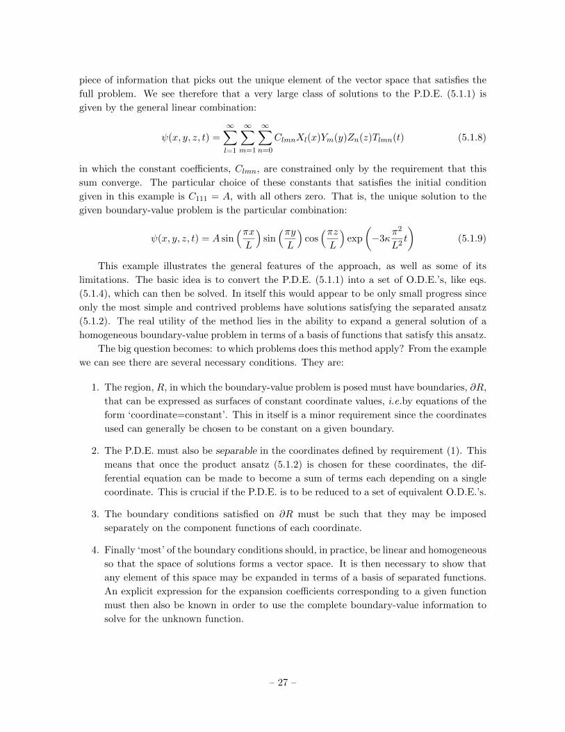
piece of information that picks out the unique element of the vector space that satisfies the
full problem. We see therefore that a very large class of solutions to the P.D.E. (5.1.1) is
given by the general linear combination:
ψ(x, y, z, t) =∞∑l=1
∞∑m=1
∞∑n=0
ClmnXl(x)Ym(y)Zn(z)Tlmn(t) (5.1.8)
in which the constant coefficients, Clmn, are constrained only by the requirement that this
sum converge. The particular choice of these constants that satisfies the initial condition
given in this example is C111 = A, with all others zero. That is, the unique solution to the
given boundary-value problem is the particular combination:
ψ(x, y, z, t) = A sin(πxL
)sin(πyL
)cos(πzL
)exp
(−3κ
π2
L2t
)(5.1.9)
This example illustrates the general features of the approach, as well as some of its
limitations. The basic idea is to convert the P.D.E. (5.1.1) into a set of O.D.E.’s, like eqs.
(5.1.4), which can then be solved. In itself this would appear to be only small progress since
only the most simple and contrived problems have solutions satisfying the separated ansatz
(5.1.2). The real utility of the method lies in the ability to expand a general solution of a
homogeneous boundary-value problem in terms of a basis of functions that satisfy this ansatz.
The big question becomes: to which problems does this method apply? From the example
we can see there are several necessary conditions. They are:
1. The region, R, in which the boundary-value problem is posed must have boundaries, ∂R,
that can be expressed as surfaces of constant coordinate values, i.e.by equations of the
form ‘coordinate=constant’. This in itself is a minor requirement since the coordinates
used can generally be chosen to be constant on a given boundary.
2. The P.D.E. must also be separable in the coordinates defined by requirement (1). This
means that once the product ansatz (5.1.2) is chosen for these coordinates, the dif-
ferential equation can be made to become a sum of terms each depending on a single
coordinate. This is crucial if the P.D.E. is to be reduced to a set of equivalent O.D.E.’s.
3. The boundary conditions satisfied on ∂R must be such that they may be imposed
separately on the component functions of each coordinate.
4. Finally ‘most’ of the boundary conditions should, in practice, be linear and homogeneous
so that the space of solutions forms a vector space. It is then necessary to show that
any element of this space may be expanded in terms of a basis of separated functions.
An explicit expression for the expansion coefficients corresponding to a given function
must then also be known in order to use the complete boundary-value information to
solve for the unknown function.
– 27 –
Property (1) can in principle be satisfied by an artful choice of coordinates given the
geometry of a specific problem. In practice, the geometries that often arise are regions that
are rectangular, cylindrical or spherical. This reflects the symmetries under translations or
rotations that underly the physics of the problem. We therefore focus explicitly on separation
of variables in cylindrical and spherical coordinates in the remainder of this chapter.
Property (2) is the key one that may or may not be satisfied by the problem of interest.
Given that it is satisfied, the demonstration of remaining properties (iii) and (iv) may be
done fairly generally and is the subject of Sturm-Liouville theory in chapter 11.
We turn now to separation of variables in cylindrical and spherical coordinates. Apart
from serving as useful examples of the method, this excercise introduces some O.D.E.’s that
arise particularly frequently, and so whose solutions are to be examined in some detail in later
chapters.
5.2 Cylindrical Coordinates
Cylindrical coordinates are most convenient for problems that are symmetric under rotations
in a plane and under translations in the direction perpendicular to that plane. The coordinates
(ρ, ξ, z, t) are related to rectangular coordinates by:
x = ρ cos ξ, 0 ≤ ξ ≤ 2π
y = ρ sin ξ, 0 ≤ ρ <∞z = z
t = t (5.2.1)
For the angular coordinate, ξ = 0 labels the same point as ξ = 2π and so any smooth
single-valued function of (x, y, z, t) must be periodic in ξ with period 2π. That is, it must be
invariant under the shift ξ → ξ + 2π.
We again take the diffusion equation (2.1.7) as our example. In cylindrical coordinates
the Laplacian operator, ∇2, defined by eq. (2.1.2) becomes:
∇2ψ =∂2ψ
∂ρ2+
1
ρ
∂ψ
∂ρ+
1
ρ2
∂2ψ
∂ξ2+∂2ψ
∂z2. (5.2.2)
so the diffusion equation is:
∂ψ
∂t− κ
[∂2ψ
∂ρ2+
1
ρ
∂ψ
∂ρ+
1
ρ2
∂2ψ
∂ξ2+∂2ψ
∂z2
]= 0. (5.2.3)
The separation ansatz in this case is:
ψ(ρ, ξ, z, t) = R(ρ)Ξ(ξ)Z(z)T (t). (5.2.4)
Substitution of (5.2.4) into (5.2.3) and division by ψ gives:
1
T
dT
dt− κ
[1
R
d2R
dρ2+
1
ρR
dR
dρ+
1
ρ2Ξ
d2Ξ
dξ2+
1
Z
d2Z
dz2
]= 0. (5.2.5)
– 28 –
The P.D.E. has become of the form: f(t) + g(ρ, ξ) +h(z) = 0 so the z- and t- dependence can
be separated as before. The t- and z-dependent parts of the equation must be constants:
dT
dt= c1T (t)
d2Z
dz2= c2Z(z) (5.2.6)
1
R
d2R
dρ2+
1
ρR
dR
dρ+
1
ρ2Ξ
d2Ξ
dξ2=c1
κ− c2
The last of these equations may be further separated if it can be put into the form f(ρ)+g(ξ) =
0. To this end multiply through by ρ2. The result has the desired form and gives the additional
separated equations:
d2Ξ
dξ2= c3Ξ
d2R
dρ2+
1
ρ
dR
dρ+c3
ρ2R+
(c2 −
c1
κ
)R = 0. (5.2.7)
The problem remains to solve these O.D.E.’s. Those for T (t), Z(z) and Ξ(ξ) are ele-
mentary and have solutions given above in eqs. (5.1.5) or (5.1.6). Furthermore, the very
definition of the coordinate ξ implies a linear and homogeneous boundary condition for Ξ:
Ξ(ξ + 2π) = Ξ(ξ). This partially determines the separation constant c3 and so gives the
following family of solutions:
Ξn(ξ) = C1 cos(nξ) + C2 sin(nξ)
c3 = −n2, n = 0,±1,±2, ... (5.2.8)
The remaining equation for R(ρ) is more difficult and the properties of its solutions are
explored in some detail in the remaining chapters. It is conventional to rewrite the O.D.E.
for R(ρ) in a more conventional form. To do so consider α2 = |c2 − c1/κ|. Changing the
independent variable to x = αρ gives:
d2R
dx2+
1
x
dR
dx+
(±1− n2
x2
)R = 0. (5.2.9)
The constant α has dropped right out of the equation. The sign ± denotes the sign of c2−c1/κ.
When the sign in (5.2.9) is positive this is called Bessel’s equation. With the negative sign it
is known as Bessel’s modified equation. Solutions to the modified equation are obtained from
solutions to Bessel’s equation by simply evaluating the result at an imaginary argument.
– 29 –
5.3 Spherical Polar Coordinates
As might be expected spherical coordinates are appropriate to problems with spherical sym-
metry. These coordinates are denoted (r, θ, φ, t) and are defined by:
x = r cosφ sin θ
y = r sinφ sin θ
z = r cos θ
t = t. (5.3.1)
The coordinates run over the range 0 < θ < π, 0 ≤ φ ≤ 2π and 0 < r < ∞. The angle
φ is periodic in the sense that φ = 0 and φ = 2π are identified. Any single-valued smooth
function must therefore be periodic under φ→ φ+ 2π.
We sketch the procedure using the diffusion equation as the illustrative example. In these
coordinates the Laplacian is:
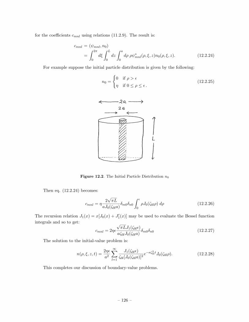
∇2ψ =1
r2
∂
∂r
(r2∂ψ
∂r
)+
1
r2 sin θ
∂
∂θ
(sin θ
∂ψ
∂θ
)+
1
r2 sin2 θ
∂2ψ
∂φ2. (5.3.2)
allowing the diffusion equation to be written:
∂ψ
∂t= κ
[1
r2
∂
∂r
(r2∂ψ
∂r
)+
1
r2 sin θ
∂
∂θ
(sin θ
∂ψ
∂θ
)+
1
r2 sin2 θ
∂2ψ
∂φ2
]. (5.3.3)
The separation ansatz is:
ψ(r, θ, φ, t) = R(r)Θ(θ)Φ(φ)T (t). (5.3.4)
Using this in eq. (5.3.3) and dividing through by ψ gives, for T , the O.D.E. of eq. (5.1.4)
together with the following equation for R, Θ and Φ:
1
Rr2
d
dr
(r2dR
dr
)+
1
Θr2 sin θ
d
dθ
(sin θ
dΘ
dθ
)+
1
Φr2 sin2 θ
d2Φ
dφ2=c1
κ. (5.3.5)
Separate the remaining variables one by one. Multiplying eq. (5.3.5) through by r2 sin2 θ
allows the φ-dependence to be separated:
d2Φ
dφ2= c2Φ(φ) (5.3.6)
andsin2 θ
R
d
dr
(r2dR
dr
)+
sin θ
Θ
d
dθ
(sin θ
dΘ
dθ
)+ c2 −
c1
κr2 sin2 θ = 0 (5.3.7)
Finally, dividing by sin2 θ separates the remaining two variables.
d
dr
(r2dR
dr
)+(c3 −
c1
κr2)R = 0 (5.3.8)
1
sin θ
d
dθ
(sin θ
dΘ
dθ
)+( c2
sin2 θ− c3
)Θ = 0. (5.3.9)
– 30 –
The O.D.E.’s for T (t), and Φ(φ) are easily solved with solutions identical to those of eqs.
(5.1.5) and, after using the boundary condition for φ, (5.2.8). The separation constant, c2 is
determined to be c2 = −m2 for m = 0,±1, ....
The solutions to eqs. (5.3.8) and (5.3.9) are more difficult to determine. We content
ourselves here to putting the remaining O.D.E.’s into canonical form. Their solutions are
found in subsequent chapters. For the equation governing Θ perform the change of variables:
x = cos θ. The range of x of physical interest is therefore −1 < x < 1. In the new variables
the O.D.E. becomes:
d
dx
[(1− x2)
dΘ
dx
]−(c3 +
m2
1− x2
)Θ = 0. (5.3.10)
This is called the Associated Legendre equation. The special case when m = 0 is Legendre’s
equation. The solution to (5.3.10) is to be found on the interval x ∈ (−1, 1). Physically, the
endpoints x = ±1 correspond to the lines θ = 0 and θ = π which label the z-axis. Since there
is nothing special about the z-axis we adopt the (homogeneous) boundary condition that Θ
not diverge even when x approaches ±1. As we shall see in chapter 10, it turns out that
the generic solution to (5.3.10) does diverge at one of the endpoints x = ±1 unless c3 takes
special values. These values are: c3 = −l(l + 1) with l = |m|, |m|+ 1, .... This result for c3 is
used for the remainder of this section.
The radial equation for R(r) is related to Bessel’s equation (5.2.9). To make this con-
nection define the new independent variable x = αr where α is defined by α =√|c1/κ|. The
radial O.D.E. is then:
1
x2
d
dx
(x2dR
dx
)+
(±1− l(l + 1)
x2
)R = 0. (5.3.11)
The upper (lower) sign ±1 in this equation corresponds to the case where c1 < 0 (c1 > 0).
The boundary conditions for R(r) usually determine this to be negative. We therefore take
the upper sign in the remainder of this chapter. Finally, performing the change of dependent
variable: y(x) = R(x)/√x gives:
d2y
dx2+
1
x
dy
dx+
(1−
(l + 12)2
x2
)y = 0 (5.3.12)
which is recognized as Bessel’s equation with n = l + 12 . Solutions to this equation are often
called spherical Bessel functions for obvious reasons.
– 31 –
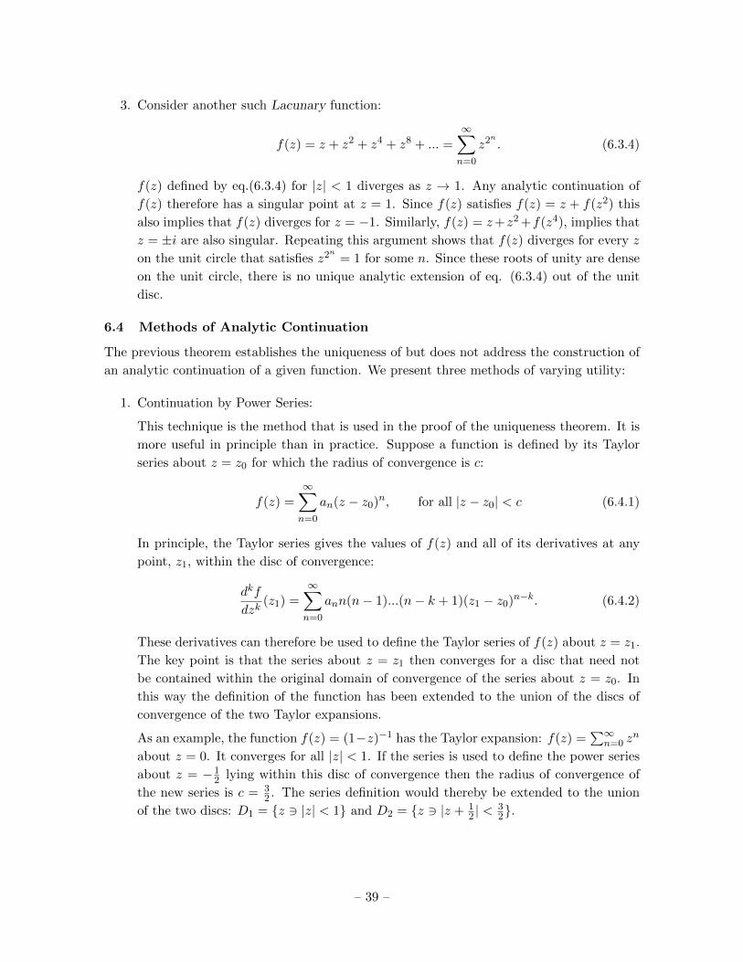
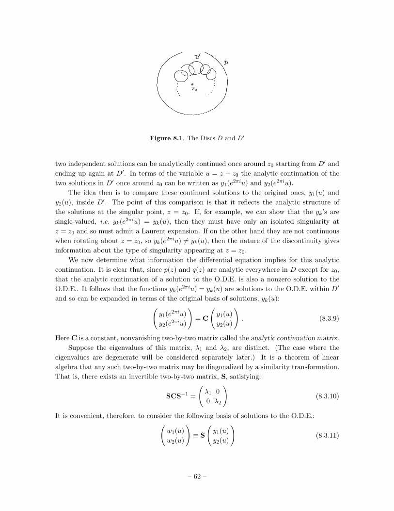
6 Complex Variables and Analytic Continuation
6.1 Introduction
The method of separation of variables has reduced the problem of constructing solutions to
the P.D.E.’s of interest to the problem of solving a set of second order, linear O.D.E.’s, of the
form:d2y
dz2+ p(z)
dy
dz+ q(z)y = f(z). (6.1.1)
What remains is to solve these O.D.E.’s. The method that we shall rely on is the construction
of solutions by power series expansion. It is therefore crucial to understand under which
circumstances such a power-series solution exists. Since the existence of a series expansion
of a function is related to the analytic properties of that function, about which the theory
of complex variables has much to say, we are led to formulate the differential equation with
both the dependent variable, y, and the independent one, z, taking complex values.
The two goals of the following sections can be simply stated. The first is to relate the
analytic properties of the solutions, y(z), of eq.(6.1.1) to the corresponding properties of the
coefficient functions, p(z) and q(z). Next, the type of O.D.E.’s that admit a series solution
must be classified and solved. In either case we first require a quick reminder of the properties
of functions of a single complex variable.
6.2 Review of the Calculus of a single Complex Variable
For convenience, some pertinent facts from the theory of the calculus of a single complex
variable are listed here.
Any complex function of a complex variable, z = x + iy, can be written as f(z, z∗) =
u(x, y)+ iv(x, y) and so is equivalent to a pair of real functions of the two real variables x and
y. f is differentiable, say, with respect to z and z∗ if and only if u and v are differentiable
with respect to x and y.
A special role is played by functions of the form f = f(z), i.e. those that are independent
of z∗. Independence of z∗ can be expressed in terms of u and v by examining the real and
imaginary parts of the condition ∂f/∂z∗ = 0:
∂u
∂x− ∂v
∂y=∂v
∂x+∂u
∂y= 0 (6.2.1)
These are called the Cauchy-Riemann equations.
Definition 6.1. Analytic function: A function, f(z), is by definition analytic at a point, z0,
if it is differentiable on a neighbourhood that includes z0. That is, the limit:
limz→z′
f(z)− f(z′)
z − z′(6.2.2)
exists, for z′ sufficiently close to z0.
– 32 –
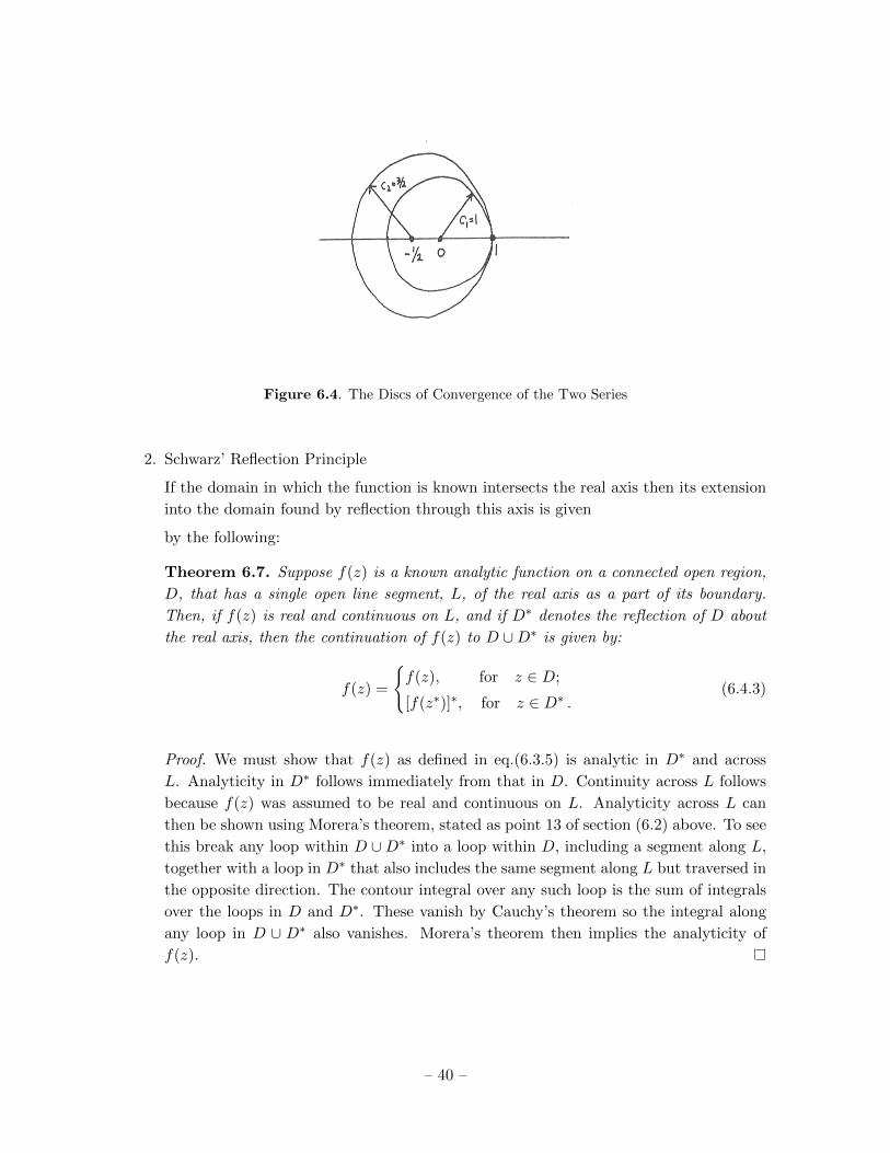
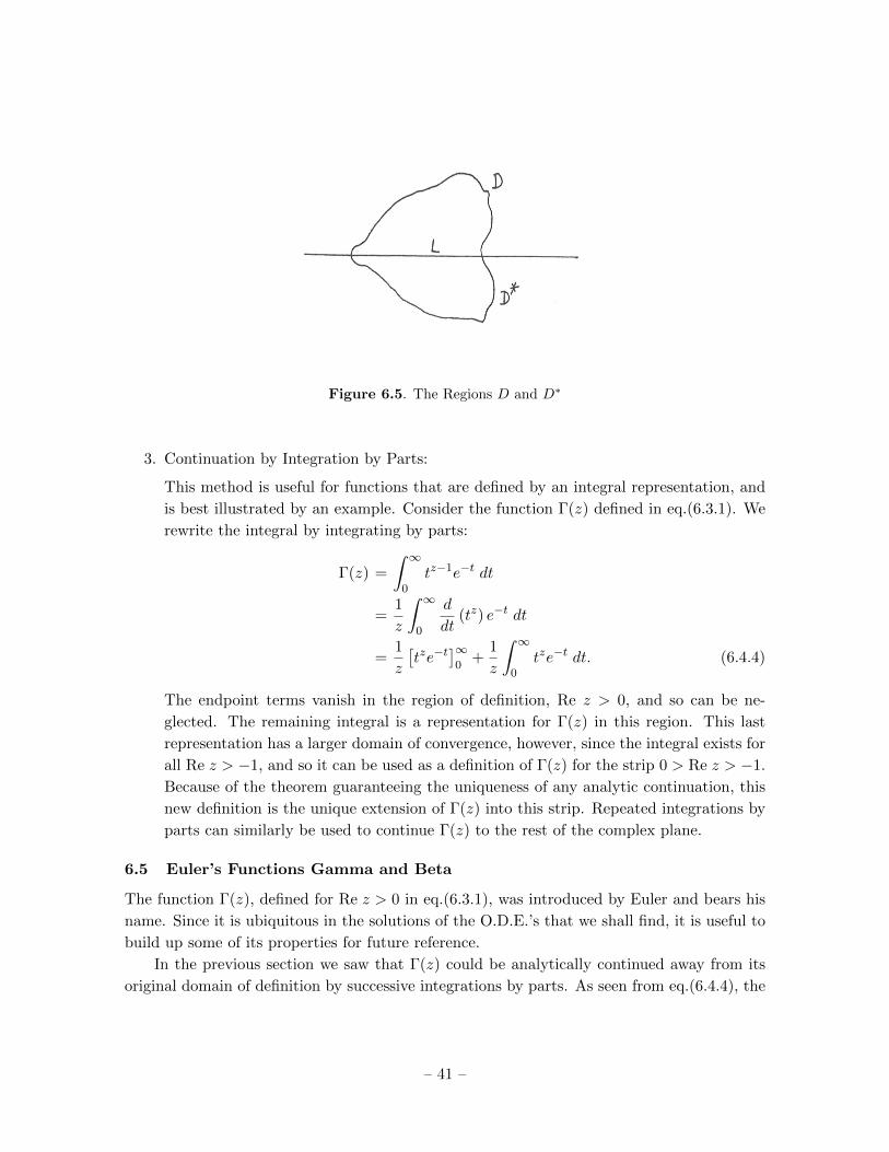
Definition 6.2. Singular Point: If f(z) is not analytic at z = z0, then z0 is called a singular
point of f(z). It is an isolated singularity if z0 lies within a disc, Dc = {z 3 |z − z0| < c},on which f(z) is analytic everywhere except for the point z = z0.
Definition 6.3. Taylor Series: If f(z) is analytic at z = z0, then there exists a disc, Dc,
centered on z0, in which its Taylor series is unique and converges uniformly to f(z):
f(z) =
∞∑n=0
an(z − z0)n ∀z ∈ Dc. (6.2.3)
The coefficients, an, in this series are found by evaluating successive derivatives at z = z0:
an =1
n!
dnf
dzn
∣∣∣∣z=z0
. (6.2.4)
Definition 6.4. Laurent Series: If f(z) is analytic throughout an annular region, Aa,b =
{z 3 a < |z − z0| < b}, surrounding the point z = z0, then its Laurent series is unique and
converges uniformly to f(z) throughout Aa,b:
f(z) =
∞∑n=0
an(z − z0)n +
∞∑n=1
bn(z − z0)n
. (6.2.5)
In particular, the Laurent series exists on a disc surrounding any isolated singularity.
Definition 6.5. Poles: An isolated singularity is called a pole of order n, for n a positive
integer, if in eq. (6.2.5) bn 6= 0 and bk = 0 for all k > n. A pole of order 1 is called a simple
pole.
Definition 6.6. Essential Singularity: An isolated singularity is called an essential singularity
if the bk-series doesn’t terminate. That is to say, for any positive integer, n, there is a k > n
such that bk 6= 0.
Definition 6.7. Entire Functions: A function, f(z), that is analytic for all finite z is called
an entire function. The Taylor expansion of an entire function about any finite point, z0,
exists for all finite z.
EXAMPLES:
a) f(z) = 1/z has a pole of order 1 at z = 0 and is analytic everywhere else.
b) f(z) = exp(1/z) =∑∞
n=01n!
(1z
)nhas an essential singularity at z = 0 and is analytic
elsewhere.
c) f(z) = log z is singular at z = 0 but the singularity is not isolated since its imaginary
part, Im log z = arg z ∈ (−π, π), is discontinuous along the negative real axis. z = 0 is called
the branch point and the line of discontinuity is called the branch cut of f(z). No Laurent
expansion exists for log z about z = 0.
– 33 –
d) f(z) = zs has an isolated singularity at z = 0 (a pole of order −s) when s is a negative
integer. If s is a nonnegative integer then zs is analytic for all finite z. If s is not an integer
then z = 0 is a singular point of zs that is not isolated since zs is not periodic in arg z. No
Laurent series exists about the branch point at z = 0, when s is not an integer.
e) f(z) = ez is an entire function.
Definition 6.8. Asymptotic Forms: A function, f(z), is bounded if there exists a positive
real number, M such that |f(z)| < M for all finite z. Similarly, a function, f(z), is said to
grow like zn as z →∞, with n a positive integer, if |f(z)| < M |z|n for all finite z.
Theorem 6.1. Liouville’s Theorem: The only entire, bounded function is the constant func-
tion: f(z) = constant.
Theorem 6.2. The only entire function that grows like zn as z → ∞ is an n-th degree
polynomial: f(z) =∑n
k=0 akzk.
Definition 6.9. Contour Integration: Suppose that f(z) is a complex function and C denotes
the path (or contour) in the complex plane that runs from z = z0 to z = z1 given by the
equations: z = c(t) = x(t) + iy(t), 0 ≤ t ≤ 1 with c(0) = z0 and c(1) = z1. The complex
contour integral, I =∫C f(z) dz, is defined by the real integral:
I =
∫ 1
0f [z(t)]
dz
dtdt
=
∫ 1
0
(u[x(t), y(t)]
dx
dt− v[x(t), y(t)]
dy
dt
)dt
+i
∫ 1
0
(u[x(t), y(t)]
dy
dt+ v[x(t), y(t)]
dx
dt
)dt. (6.2.6)
Theorem 6.3. Cauchy-Goursat Theorem: Suppose C denotes a closed curve given by the
equation: z = c(t), 0 ≤ t ≤ 1 with c(0) = c(1). If f(z) is analytic at all points on and within
C then: ∫Cf(z) dz = 0. (6.2.7)
Notice that this implies that the contour integral along any two curves, C1 and C2, joining
the points z0 and z1 in the complex plane must agree provided that the region between the two
contours doesn’t contain a singular point of the integrand. To see this notice that traversing
contour C1 from t = 0 to t = 1 and then traversing C2 backwards from t = 1 to t = 0 amounts
to travelling once around a closed contour, C. Therefore:∫C1
f(z) dz −∫C2
f(z) dz =
∫Cf(z) dz = 0 (6.2.8)
A different way of expressing the same conclusion is that a complex integral is unchanged as
the contour of integration is ‘deformed’ all around the complex plane provided only that the
deformations never take the contour across a singular point of the integrand.
– 34 –
Figure 6.1. The Contours C1, C2 and C
Theorem 6.4. Morera’s Theorem: This is the converse to Cauchy’s theorem. If∫C f(z) dz =
0 for all closed curves, C, in a connected open domain, D, then f(z) is analytic throughout
D.
Definition 6.10. Residues: If z = z0 is an isolated singularity of an analytic function, f(z),
with Laurent expansion given by eq.(6.2.5), then the residue of f(z) at z0 is defined as the
value of the coefficient b1. Notice that if f(z) has a simple pole at z0 then inspection of the
Laurent series shows that the residue is given by:
B = limz→z0
[(z − z0)f(z)] = limz→z0
[ ∞∑n=0
an(z − z0)n+1 + b1
]= b1. (6.2.9)
Theorem 6.5. Residue Theorem: If C is a closed contour within and on which a function,
f(z), is analytic except at a finite number of isolated singular points, {z1, z2, ..., zn} in the
in which the integration traverses C in the counterclockwise sense and Bk denotes the residue
of f(z) at the point zk.
EXAMPLES:
a) Suppose f(z) = 1/z is integrated about the closed contour C : c(t) = exp(2πit) for
0 ≤ t ≤ 1. This equation describes the unit circle traversed once counterclockwise starting
from z0 = c(0) = 1. The integral is∫C(1/z) dz = 2πi
∫ 10 dt = 2πi. This agrees with the
residue theorem since f(z) = 1/z has a simple pole in the interior of C at z = 0 with residue
B = 1.
– 35 –
Figure 6.2. The Contour C
b) If f(z) = 1/z2 is integrated over the same contour as in the previous example, the
result is∫C(1/z2) dz = 2πi
∫ 10 e−2πit dt = 0. This also agrees with the residue theorem
because f(z) = 1/z2 has an isolated singular point at z = 0 but with residue B = 0.
c) This final example gives a contour integral representation for a series. It provides a
powerful method for evaluating series. Consider the series, S =∑∞
n=−∞ an. Suppose there
exists a function, f(z), that is analytic near the real axis and which satisfies f(z = n) = an.
An integral representation of the series, S, is furnished by:
S =1
2i
∫Cf(z) cot(πz) dz (6.2.11)
in which the contour, C, runs from −∞ to ∞ just below the real axis and returns from ∞ to
−∞ just above the real axis. The interior of this contour is a narrow strip centered on the
real axis.
To establish the validity of eq.(6.2.11) we evaluate the integral along C by residues.
The only poles of the integrand are, by assumption, those of the cotangent factor and these
consist of simple poles for integer z = n. The residue of the integrand at these poles is (using
l’Hopital’s rule and point 14 above):
Bn = limz→n
(z − n)f(z)
tan(πz)= lim
z→n
f(z)
π sec2(πz)=f(n)
π. (6.2.12)
so the residue theorem gives:
1
2i
∫Cf(z) cot(πz) dz = π
∞∑n=−∞
Bn =
∞∑n=−∞
f(n) = S. (6.2.13)
as required.
This completes the brief summary of the calculus of a complex variable.
– 36 –
6.3 Analytic Continuation: Uniqueness
It will rarely be possible to express the solutions to the O.D.E.’s of interest in closed form.
They will instead be exhibited as a power series or in an integral representation. Such
representations are generally well-defined only for a restricted region of the complex plane, R
say, in which the sum or integral converges. It is in order to extend this kind of representation
to more general regions that the notion of analytic continuation is required.
Statement of the problem:
Suppose a function is defined via an integral representation. For example:
Γ(z) =
∫ ∞0
tz−1e−t dt (6.3.1)
defines a function, Γ(z), within the region of convergence of the integral: Re z > 0. This
function is analytic within this region since
dΓ
dz=
∫ ∞0
tz−1e−t log t dt (6.3.2)
also converges for Re z > 0. The problem is: can such a definition of a function be extended
in a reasonable (unique) way to the entire complex plane? Although in general there is no
such natural extension, it is possible in many cases of interest. The main result takes the
form of the following:
Theorem 6.6. If two functions, f1(z) and f2(z), are analytic in a connected open region,
D1, of the complex plane, and if f1 = f2 for all z in a connected open region D2 ⊂ D1, then
f1 = f2 throughout all of D1.
This states that if an analytic function is known on a complex region, D2, and if it can
be extended to an analytic function throughout a larger region, D1, that includes D2, then
that extension is unique. The extension of an analytic function from D2 to D1 is known as
an analytic continuation.
Proof. (Rather, Sketch of Proof):
To get a flavour for the argument, we present a sketch of the proof of the theorem.
Consider the function g(z) = f1(z)−f2(z). By assumption this function is analytic throughout
the larger region, D1, and vanishes throughout D2. The argument is to show that these
conditions imply that g(z) vanishes throughout D1. To show this choose any point, ζ, that
lies within D1 but not D2, and choose a curve, C, that connects ζ to some point, z0, within
D2. By assumption g(z) is analytic along some strip of width 2w contained within D1 and
centered on the curve C. This implies that g(z) admits a Taylor series expansion about any
point of C whose radius of convergence is at least w.
The idea is now to consider a sequence of n overlapping discs of radius w and centered
at points, zk, that lie on C. We require that the first point be z0 ∈ D2, that the last point be
– 37 –
Figure 6.3. The n Overlapping Discs
zn−1 = ζ and that each point, zk, lies within the neighbouring two discs. Since g(z) vanishes
throughout D2 it vanishes within the first disc and so its Taylor series there is zero. This
implies that g(z) vanishes on the overlap with the next disc and so its power series there must
also be zero. Since this series is unique, it and g(z) must therefore vanish throughout the
entire disc centered at z1. Proceeding in an identical fashion implies that g(z) vanishes within
all of the discs and so also at ζ. Repeating this argument for any point, ζ, in D1 implies that
g(z) vanishes throughout D1 as required.
Before moving on to the construction of analytic continuations of given functions we
consider a few examples that cannot be analytically continued.
1. f(z) = log z = log |z|+i arg z for D = {z 3 −π < arg z < π}. If an analytic continuation
to the entire plane were to exist it would have to be given by this same expression since
it is unique and must agree with f(z) everywhere in D. Since this expression is not
continuous across the negative real axis, an analytic continuation cannot exist.
2. Consider the function defined for Im z > 0 by:
f(z) =∞∑n=0
∞∑m=−∞
′e−(m2+n2)
mz − n. (6.3.3)
The prime denotes the omission of the term m = n = 0 from the sum. As defined f(z)
is analytic for all Im z > 0 and has poles at every rational number on the real axis:
z = n/m. Since any neighbourhood of any real number contains a rational number (i.e.
the rational numbers are dense in the reals) it is impossible to define a finite-width strip
that crosses the real axis and on which f(z) is analytic. As a result the uniqueness
theorem fails and there is no unique way to analytically extend f(z) below the real axis.
– 38 –
3. Consider another such Lacunary function:
f(z) = z + z2 + z4 + z8 + ... =∞∑n=0
z2n . (6.3.4)
f(z) defined by eq.(6.3.4) for |z| < 1 diverges as z → 1. Any analytic continuation of
f(z) therefore has a singular point at z = 1. Since f(z) satisfies f(z) = z + f(z2) this
also implies that f(z) diverges for z = −1. Similarly, f(z) = z+z2 +f(z4), implies that
z = ±i are also singular. Repeating this argument shows that f(z) diverges for every z
on the unit circle that satisfies z2n = 1 for some n. Since these roots of unity are dense
on the unit circle, there is no unique analytic extension of eq. (6.3.4) out of the unit
disc.
6.4 Methods of Analytic Continuation
The previous theorem establishes the uniqueness of but does not address the construction of
an analytic continuation of a given function. We present three methods of varying utility:
1. Continuation by Power Series:
This technique is the method that is used in the proof of the uniqueness theorem. It is
more useful in principle than in practice. Suppose a function is defined by its Taylor
series about z = z0 for which the radius of convergence is c:
f(z) =∞∑n=0
an(z − z0)n, for all |z − z0| < c (6.4.1)
In principle, the Taylor series gives the values of f(z) and all of its derivatives at any
point, z1, within the disc of convergence:
dkf
dzk(z1) =
∞∑n=0
ann(n− 1)...(n− k + 1)(z1 − z0)n−k. (6.4.2)
These derivatives can therefore be used to define the Taylor series of f(z) about z = z1.
The key point is that the series about z = z1 then converges for a disc that need not
be contained within the original domain of convergence of the series about z = z0. In
this way the definition of the function has been extended to the union of the discs of
convergence of the two Taylor expansions.
As an example, the function f(z) = (1−z)−1 has the Taylor expansion: f(z) =∑∞
n=0 zn
about z = 0. It converges for all |z| < 1. If the series is used to define the power series
about z = −12 lying within this disc of convergence then the radius of convergence of
the new series is c = 32 . The series definition would thereby be extended to the union
of the two discs: D1 = {z 3 |z| < 1} and D2 = {z 3 |z + 12 | <
32}.
– 39 –
Figure 6.4. The Discs of Convergence of the Two Series
2. Schwarz’ Reflection Principle
If the domain in which the function is known intersects the real axis then its extension
into the domain found by reflection through this axis is given
by the following:
Theorem 6.7. Suppose f(z) is a known analytic function on a connected open region,
D, that has a single open line segment, L, of the real axis as a part of its boundary.
Then, if f(z) is real and continuous on L, and if D∗ denotes the reflection of D about
the real axis, then the continuation of f(z) to D ∪D∗ is given by:
f(z) =
{f(z), for z ∈ D;
[f(z∗)]∗, for z ∈ D∗ .(6.4.3)
Proof. We must show that f(z) as defined in eq.(6.3.5) is analytic in D∗ and across
L. Analyticity in D∗ follows immediately from that in D. Continuity across L follows
because f(z) was assumed to be real and continuous on L. Analyticity across L can
then be shown using Morera’s theorem, stated as point 13 of section (6.2) above. To see
this break any loop within D ∪D∗ into a loop within D, including a segment along L,
together with a loop in D∗ that also includes the same segment along L but traversed in
the opposite direction. The contour integral over any such loop is the sum of integrals
over the loops in D and D∗. These vanish by Cauchy’s theorem so the integral along
any loop in D ∪ D∗ also vanishes. Morera’s theorem then implies the analyticity of
f(z).
– 40 –
Figure 6.5. The Regions D and D∗
3. Continuation by Integration by Parts:
This method is useful for functions that are defined by an integral representation, and
is best illustrated by an example. Consider the function Γ(z) defined in eq.(6.3.1). We
rewrite the integral by integrating by parts:
Γ(z) =
∫ ∞0
tz−1e−t dt
=1
z
∫ ∞0
d
dt(tz) e−t dt
=1
z
[tze−t
]∞0
+1
z
∫ ∞0
tze−t dt. (6.4.4)
The endpoint terms vanish in the region of definition, Re z > 0, and so can be ne-
glected. The remaining integral is a representation for Γ(z) in this region. This last
representation has a larger domain of convergence, however, since the integral exists for
all Re z > −1, and so it can be used as a definition of Γ(z) for the strip 0 > Re z > −1.
Because of the theorem guaranteeing the uniqueness of any analytic continuation, this
new definition is the unique extension of Γ(z) into this strip. Repeated integrations by
parts can similarly be used to continue Γ(z) to the rest of the complex plane.
6.5 Euler’s Functions Gamma and Beta
The function Γ(z), defined for Re z > 0 in eq.(6.3.1), was introduced by Euler and bears his
name. Since it is ubiquitous in the solutions of the O.D.E.’s that we shall find, it is useful to
build up some of its properties for future reference.
In the previous section we saw that Γ(z) could be analytically continued away from its
original domain of definition by successive integrations by parts. As seen from eq.(6.4.4), the
– 41 –
result has the property that:
Γ(z) =Γ(z + 1)
z= ... =
Γ(z + n+ 1)
z(z + 1) . . . (z + n)(6.5.1)
for any positive integer, n. Since, by explicit evaluation, Γ(1) =∫∞
0 exp(−t) dt = 1, we see
that property (6.5.1) ensures that Γ(k + 1) = k! for any positive integer, k. Similarly, since
it was by definition analytic in the region Re z > 0, eq.(6.5.1) implies that Γ(z) is analytic
everywhere except for simple poles at z = 0,−1,−2, .... Its residue at z = −n is given by:
Bn = limz→−n
[(z + n)Γ(z)] =Γ(1)
(−n)(1− n)(2− n) . . . (−1)=
(−)n
n!. (6.5.2)
Another useful function of Euler’s is the Beta function, B(α, β), defined by:
B(α, β) =
∫ 1
0(1− t)α−1tβ−1 dt. (6.5.3)
This definition converges provided that Re α > 0 and Re β > 0. An alternative way to write
eq.(6.5.3) is found by performing the change of variables t = sin2 θ in terms of which:
B(α, β) = 2
∫ π/2
0cos2α−1 θ sin2β−1 θ dθ. (6.5.4)
The next step is to extend this definition to the remainder of the complex plane. Rather
than working directly with the integral representation we make a connection to Γ(z). To do
this consider the product:
Γ(α)Γ(β) =
∫ ∞0
du
∫ ∞0
dv uα−1e−uvβ−1e−v (6.5.5)
Changing variables to u = x2 and v = y2 and then switching to polar coordinates x = r cos θ
and y = r sin θ gives the following:
Γ(α)Γ(β) = 4
[∫ ∞0
dr r2α+2β−1e−r2
][∫ π/2
0dθ cos2α−1 θ sin2β−1 θ
](6.5.6)
Changing variables to t = r2 and comparing to the definition (6.3.1) shows that the first factor
is equal to 12Γ(α+ β). The second factor, on the other hand, when compared to eq.(6.5.4), is
equal to 12B(α, β). Combining these relations and solving for B(α, β) gives the equation:
B(α, β) = B(β, α) =Γ(α)Γ(β)
Γ(α+ β). (6.5.7)
Although this last equation has been derived for positive Re α and Re β, for which the
integral representations converge, it must hold for all complex α and β. This is because both
sides of eq.(6.5.7) are analytic and the left-hand-side agrees with the definition, (6.5.2) within
its domain of validity. Since the analytic continuation of eq.(6.5.2) is unique, it must be given
by eq.(6.5.7) away from the original domain of definition.
In order to further illustrate complex-variable techniques and for further use we now
develop some properties of the Γ-function.
– 42 –
1. Reflection Formula:
Γ(z)Γ(1− z) =π
sin(πz)(6.5.8)
In order to prove the validity of eq.(6.5.8) consider the beta-function evaluated at α = z
and β = 1− z. Using Γ(1) = 1 gives:
Γ(z)Γ(1− z) = B(1− z, z) =
∫ 1
0tz−1(1− t)−z dt (6.5.9)
in which the final integral representation converges for 0 < Re z < 1. The logic is
to use this integral representation to prove relation (6.5.8) within the strip in which it
converges and then to use the uniqueness of analytic continuation to infer that the result
also holds in the remainder of the complex plane. The change of variables t = u/(u+ 1)
in (6.5.9) produces the following integral:
B(z, 1− z) =
∫ ∞0
uz−1
1 + udu. (6.5.10)
The idea is to explicitly evaluate this integral by residues. In order to do so we need to
know the singularities of the integrand. By inspection the integrand has a simple pole
at u = −1 and, for z not an integer, a branch point at u = 0. We can choose to define
uz = exp(z log u) with log u = log |u| + i arg u and 0 < arg u < 2π. This amounts to
choosing the branch cut to lie along the positive real axis.
Consider, then, the integral (6.5.10) evaluated along the contour C = {z 3 z = −1 +12e
2πit} consisting of a circle with radius 12 centered on the pole at u = −1 and traversed
in the counterclockwise sense. This integral is easily evaluated by residues and gives:
I ≡∫C
uz−1
1 + udu = −2πi exp(iπz). (6.5.11)
The argument now relies on deforming the contour, C, to a new contour, C ′, that is
related to the range of integration of the integral in eq.(6.5.10). The new contour is
given by C ′ = C∞ ∪ C− ∪ C0 ∪ C+ where the segments are defined as the limit of the
following contours as R→∞ and r → 0:
C∞ = {u = Re2πit, 0 ≤ t ≤ 1};C− = {u = R(1− t)− ir, 0 ≤ t ≤ 1};C0 = {u = reiπ(
32−t), 0 ≤ t ≤ 1};
C+ = {u = Rt+ ir, 0 ≤ t ≤ 1}; (6.5.12)
The claim is that the contribution to the integral from the contours C∞ and C0 vanish
in the limit that r → 0 and R → ∞. The sole contribution to the integral along C ′ is
– 43 –
Figure 6.6. The Contours Referred to in the Proof
therefore from the integrals on either side of the branch cut, C±. These integrals are
related to the integral (6.5.10) that we wish to compute.
The first step is to show that the arcs ‘at infinity’ and ‘at zero’ contribute nothing.
Consider the contribution of C∞. We have:
A ≡ limR→∞
A(R)
with A(R) =
∫ 1
0
Rz−1e2πit(z−1)
1 +Re2πitRe2πit2πi dt
= 2πiRz∫ 1
0
e2πitz
1 +Re2πitdt (6.5.13)
The vanishing of this limit is proven by bounding the absolute value |A(R)| from above
by a function that vanishes as R → ∞. The desired inequality follows from repeated
use of the triangle inequality.
|A(R)| ≤ 2πRRe z∫ 1
0
e−2πtIm z
|1 +Re2πit|dt
≤ 2πRRe z
R− 1
∫ 1
0e−2πtIm z dt (6.5.14)
The first inequality is an application of the triangle inequality in its integral form:∣∣∫ f(t) dt∣∣ ≤ ∫ |f(t)| dt. The second follows from the triangle inequality applied to the
denominator of the integrand: |1 +R exp(2πit)| ≥ R− 1. The remaining integral in the
final line of eq. (6.5.14) is elementary. It remains to perform the limit R → ∞. The
key observation is that we have required that z lie in the strip 0 < Re z < 1. With this
choice the right-hand-side of eq. (6.5.14) vanishes when R becomes arbitrarily large, so
A = limR→∞A(R) = 0 as required.
– 44 –
An identical argument may be applied to the semicircular arc near the origin:
B = limr→0
B(r)
with B(r) = −iπrz∫ 1
0
eiπz(32−t)
1 + reiπ(32−t)
dt
so |B(r)| ≤ πrRe z
1− r
∫ 1
0e−πIm z( 3
2−t) dt (6.5.15)
The limit as r → 0 of the right-hand-side of the last equation in (6.5.15) is zero for any
0 < Re z < 1. This demonstrates that B(r) vanishes in this limit and so, therefore,
does B.
The remaining contribution to the contour integral around C ′ is from the segments just
above and below the positive real axis. This gives:
I =
∫C′
uz−1
1 + udu
=
∫C+
uz−1
1 + udu+
∫C−
uz−1
1 + udu
= limr→0
∫ ∞0
[(t+ ir)z−1
1 + t+ ir− (t− ir)z−1
1 + t− ir
]dt
=[1− e2πiz
] ∫ ∞0
tz−1
1 + tdt (6.5.16)
Notice that the integral on the right-hand-side of this final equation is precisely the
integral of eq. (6.5.10) that we wish to evaluate. Combining, then, eqs. (6.5.10),
(6.5.11) and (6.5.16) allows the desired conclusion:
Γ(z)Γ(1− z) =
∫ ∞0
tz−1
1 + tdt
=1
1− e2πiz
∫C′
uz−1
1 + udu
=−2πieiπz
1− e2πiz
=π
sin(πz). (6.5.17)
As indicated earlier, even though this result has only been proven for z lying within
the strip 0 < Re z < 1 its validity follows for the rest of the complex z-plane by
virtue of the uniqueness of analytic continuation. That is, both sides of eq. (6.5.17) are
analytic apart from isolated poles throughout the plane and they agree within the strip
0 < Re z < 1. They must therefore agree throughout the rest of the plane.
An important special case of the reflection formula is obtained by choosing z = 12 . In
this case it reads [Γ(12)]2 = π. Since the integral formula (6.4.4) implies that Γ(1
2) > 0,
– 45 –
it follows that Γ(12) =
√π. Repeated use of property Γ(z+1) = zΓ(z) that follows from
eq. (6.5.1) gives, for Γ evaluated at any half-odd number 1:
Γ
(n+
1
2
)=
(2n− 1)!!
2n√π. (6.5.18)
The next property to be proven for the Γ-function relates its value at 2z to its value at
z and z + 12 .
2. Duplication Formula:
Γ(z)Γ
(z +
1
2
)= 21−2z√π Γ(2z) (6.5.19)
This result follows from an artful choice of variables in the integral representation of
the beta-function. Consider, for Re z > 0:
B(z, z) =[Γ(z)]2
Γ(2z)=
∫ 1
0tz−1(1− t)z−1 dt. (6.5.20)
Change variables to v = (2t− 1)2. As t varies from 0 to 1 v covers the region from 0 to
1 twice. The resulting integral is:
B(z, z) = 21−2z
∫ 1
0v−
12 (1− v)z−1 dv
= 21−2zB
(1
2, z
)= 21−2zΓ(z)Γ(1
2)
Γ(z + 12). (6.5.21)
The duplication formula is now obtained by multiplying eq. (6.5.21) through by Γ(2z)Γ(z+12)/Γ(z). As usual, although the proof of this result used the assumption that Re z > 0,
both sides of the final equation are analytic and so the uniqueness theorem for analytic
continuation ensures that the duplication formula holds for all z.
The final property of Euler’s Γ-function that is to be proven is Stirling’s Formula and is
the subject of the next chapter.
1(2n− 1)!! = (2n− 1)(2n− 3) · · · 3 · 1.
– 46 –
7 Asymptotic Forms and the Method of Steepest Descent
For many purposes it is useful to be able to describe the behaviour of a given function for
large values of its argument. It is of particular use to be able to do so even when the
function is defined by a series or integral representation, as are the solutions we construct
to the O.D.E.’s in later chapters. For integral representations a very useful technique for
generating such asymptotic forms is the method of Steepest Descent. (This method is also
often referred to as the Stationary-Phase Approximation or the Saddle-Point Approximation.)
This technique is described in this chapter in its simplest possible setting. It is worth keeping
in mind, however, that the technique has a more general setting and is much more powerful
than might appear from the presentation below.
7.1 The Approximation
We encounter the saddle-point approximation within the context of deriving the behaviour
of Γ(z) for large values of z. The result is expressed by
Stirling’s Formula:
Γ(z + 1) =√
2πzz+12 e−z
[1 +
1
12z+
1
288z2+O(z−3)
](7.1.1)
Formula (7.1.1) is derived with the help of the integral representation, (6.3.1), that defines
Γ(z) and is applicable for Re z > 0. The first step in doing so is to change variables to u = t/z
and rotate the resulting contour of integration back to the positive real axis.
Γ(z + 1) =
∫ ∞0
tze−t dt
= zz+1
∫ ∞0
ez(log u−u) du (7.1.2)
This form for the integrand is the one for which the method of steepest descent may apply,
namely to integrals of the form:
I(z) =
∫ ∞0
ezf(u) du. (7.1.3)
In the case at hand the real function f(u) is given by f(u) = log u − u. In this more
general case we wish to know the behaviour of I(z) as z →∞. (In general it is not necessary,
for the method of steepest descent, for f(u) to be real or for the integration range to consist
only of the positive real axis.) f(u) must go to −∞ sufficiently quickly as u → ∞ if this
integral to converge. We also assume that f(u) also has a single stationary point which is a
global maximum for some u 6= 0. This last assumption is again not necessary but is chosen
to simplify the argument.
It is easy to see that this function has a single stationary point at u = 1 where f ′(1) =
[u−1−1]|u=1 = 0 and f(1) = −1. This corresponds to a global maximum. The function falls off
– 47 –
to negative infinity as u→ 0 and as u→∞, and the second derivative is f ′′(u) = −1/u2 < 0 so
it is everywhere concave downwards. The Taylor expansion of f(u) about u = 1 is elementary
and is given for |u− 1| < 1 by:
f(u) = −1−∞∑n=2
(−)n
n(u− 1)n. (7.1.4)
Here’s the essence of the argument. For larger and larger Re z the integrand, ezf(u), is
more and more strongly peaked about the stationary point of f(u) at u = 1. It should there-
fore follow that the behaviour of I(z) for such large z is completely governed by the behaviour
of the integrand in the neighbourhood of the stationary point u = 1. A good approximation
should therefore be obtained by Taylor-expanding the argument of the exponent about this
point, using eq. (7.1.4). The first term of this series that depends on u − 1 is quadratic.
The idea is to leave this term in the exponent to ensure that the integral over u converges
for large u but to again Taylor-expand the exponential of the remainder of the series and to
then integrate the result term-by-term. The final claim is that the resulting function of z so
obtained furnishes an asymptotic series for I(z) of the form:
I(z) = A(z)
[1 +
B
z+O(z−2)
]. (7.1.5)
We illustrate this method by using it to calculate Stirling’s formula, (7.1.1). A demonstration
that the terms neglected in the derivation are negligible, i.e. that the result is an asymptotic
series, is sketched at the end.
Writing the Taylor expansion of eq. (7.1.4) as f(u) = −1 − 12(u − 1)2 − S(u), in which
S(u) =∑∞
n=3(−)n
n (u− 1)n denotes all of the terms beyond second order in (u− 1), allows the
argument of the integrand to be written:
exp[zf(u)] = exp
[−z − 1
2z(u− 1)2 − zS(u)
]= e−z exp
[−1
2z(u− 1)2
]exp [−zS(u)]
= e−z exp
[−1
2z(u− 1)2
] ∞∑k=0
1
k![−zS(u)]k
= e−z exp
[−1
2z(u− 1)2
][1− z
( ∞∑n=3
(−)n
n(u− 1)n
)
+1
2z2
( ∞∑n=3
(−)n
n(u− 1)n
)2
+ ...
(7.1.6)
– 48 –
I(z) is to be constructed by integrating the last result of eqs. (7.1.6) term-by-term. This
gives the unwieldy result:
I(z) = e−z
[∫ ∞0
e−12z(u−1)2 du− z
∞∑n=3
(−)n
n
∫ ∞0
e−12z(u−1)2(u− 1)n du+
+1
2z2∞∑n=3
∞∑m=3
(−)n+m
mn
∫ ∞0
e−12z(u−1)2(u− 1)n+m du+ ...
](7.1.7)
Since the integral is dominated, for large Re z, by the behaviour of the integrand near
u = 1 the lower limit of integration may be taken to be negative infinity rather than zero with
negligible error. (More about the size of this error later.) The integrals are then straightfor-
ward and may be evaluated in terms of Euler’s Γ-function. Using the variable t = 12z(u− 1)2
and rotating the contour back onto the real axis gives:∫ ∞−∞
e−12z(u−1)2(u− 1)p du = 0 if p = 2n+ 1
=
(2
z
)n+ 12∫ ∞
0e−ttn−
12 dt if p = 2n
=
(2
z
)n+ 12
Γ
(n+
1
2
)(7.1.8)
Using eq. (7.1.8) in eq. (7.1.7) gives:
I(z) =
(2
z
) 12
e−z
{Γ(
1
2)− z
∞∑n=2
(1
2n
)(2
z
)nΓ
(n+
1
2
)+
+1
2z2
∞∑n=3
∞∑m=3
′(1
mn
)(z2
)− 12
(m+n)Γ
[1
2(m+ n+ 1)
]+ ...
}(7.1.9)
The prime on the sum indicates that only those terms with n+m even are to be included.
Collecting the first few powers of 1/z and using eq. (6.5.18) for Γ(p+ 12) gives:
I(z) =
(2π
z
) 12
e−z
[1−
∞∑n=2
(2n− 1)!!
2nz1−n+
+∞∑n=3
∞∑m=3
′(m+ n− 1)!!
2mnz2− 1
2(m+n) + ...
]
=
(2π
z
) 12
e−z[1 +
1
12z+
1
288z2+ ...
](7.1.10)
Inserting this asymptotic form for I(z) into Γ(z+ 1) = zz+1I(z) reproduces the first terms of
Stirling’s formula.
– 49 –
What remains to be shown is that the approximations employed in deriving eq. (7.1.10)
only contribute terms that are small. The claim is that the inclusion of higher powers of
(u− 1) in the series for exp[−zS(u)] only adds corrections to (7.1.10) that are O(z−3). The
remaining approximations, such as that of changing the lower limit of integration in eq.
(7.1.7) to negative infinity, introduce an error that is smaller than any power of z: i.e. they
are o(z−n) for any n.
7.2 The Accuracy of the Approximation
The claim to be demonstrated is that the series (7.1.10) in 1/z is an asymptotic series for the
function I(z). That is, it remains to prove the following:
A1(z) ≡ I(z)√2πz e−z− 1 = O(z−1)
A2(z) ≡ A1(z)− 1
12z= O(z−2) (7.2.1)
and so on.
Proof. In order to simplify the argument and to avoid a mathematical technicality a slightly
easier proposition than this will be argued. The simplification is to establish eq. (7.2.1a),
say, for the proper integral
A1[0, R; z] ≡√
z
2πe−zf(u0)
∫ R
0ezf(u) du (7.2.2)
rather than the original improper integral in which the upper limit, R, is taken to infinity.
The argument in the more general case of interest requires some modification but is basically
equivalent.
The result is demonstrated by dividing the integration into two regions: one lying within
a neighbourhood (u0− ε, u0 + ε) surrounding the stationary point u0 and the other consisting
It is furthermore an independent solution since explicit differentiation of Y (s; z) gives:
y2(z) = y1(z) log(z − z0) +
∞∑n=0
(∂yn(s)
∂s
)s=α
(z − z0)n+α. (8.5.12)
y2(z) must be linearly independent of y1(z) because otherwise they would be propor-
tional to one another. However they cannot be proportional to one another since y2(z)
has a logarithmic singularity as z → z0 which y1(z) does not share.
– 70 –
2. s2 = α and s1 = α − N for N a positive integer: In this case we must use a slight
modification of the same trick. Consider again the function Y (s; z), defined just as
before by (8.5.8) in which the recursion relations are imposed but the parameter s is
kept arbitrary. The known solution is in this case obtained by evaluating Y (s; z) at
s = α: y1(z) = Y (α; z). We are interested in the case where evaluation at s = α − Ndoes not generate the second solution because the recursion relation implies yN (α−N)
is infinite. This shows up in the function Y (s; z) as a simple pole for yN (s) at s = α−Nas is seen from eq. (8.4.12):
yN (s) =FN [s; y0, ..., yN−1]
I(s+N)=
FN [s; y0, ..., yN−1]
(s− α+N)(s− α+ 2N). (8.5.13)
In this case the action of the operator L on Y (s; z) is:
which is in Hypergeometric form with a+ b = 1 + 2m, ab = t+m+m2 and c = 1 +m. This
has solutions a = 12(1 + 2m ±
√1− 4t) and b = 1
2(1 + 2m ∓√
1− 4t). It does not matter
whether the upper or lower sign is chosen in these expressions for a and b since changing this
sign just has the effect of switching a and b and the Hypergeometric equation is unchanged
by such a switch.
The relation between the solutions to this O.D.E. and those of the original O.D.E. is:
y = [w(w − 1)]m/2v(w) = 2−meiπm/2(1− z2)m/2v
[1
2(1− z)
]. (9.4.9)
EXAMPLE 2: Bessel’s equation, (5.2.9):
y′′(z) +1
zy′(z) +
(1− ν2
z2
)y(z) = 0. (9.4.10)
ν is in general a complex constant.
This equation has two singular points, a regular one at z = 0 and an irregular one
at z = ∞. It is therefore potentially equivalent to the Confluent Hypergeometric equation
(9.3.2). In principle, the strategy to be followed is the same as for the Hypergeometric
equation. We perform the most general change of variables u = u(z) and y(u) = f(u)v(u)
consistent with the requirement that (i) no new singularities are introduced, and (ii) that
the existing singularities not be moved from their standard places (z = 0 and z = ∞ in the
present example). The requirement that the O.D.E. in the new variables have the standard
form then imposes conditions on the unknown functions f(z) and u(z) that can be solved.
The resulting values for the constants a and c in the standard form can then be read off by
inspection.
Unfortunately, since there is no general theorem stating that any O.D.E. with one regular
and one irregular singular point can be put into Confluent Hypergeometric form, it may be
that there is no change of variables that can transform the O.D.E. to the desired form. If
not, then the complete set of conditions required of u(z) and f(z) will be found to have no
solution.
In the present example we are allowed to perform any one-to-one transformation u(z) of
the complex plane to itself that does not move the singular points: u(0) = 0, u(∞) = ∞.
Furthermore, u(z) must be analytic everywhere, except potentially at z = 0 and z =∞, if it
is not to introduce any new singular points apart from those at z = 0 and z =∞. At z = 0
the potentially singular behaviour of u(z) is constrained by the requirement that the singular
point not become irregular once expressed in terms of the new variable.
In order to do this analysis properly an analogue of the theorems (1) and (2) of section 9.2
are required. These are more difficult to identify in this case since the behaviour as z → ∞
– 80 –
is not restricted in the present example. Rather than trying to derive the most general
transformation, then, we content ourselves with an educated guess of which transformations
to try. To this end, notice that one type of transformation that satisfies all of the above
conditions, though not necessarily the most general type, is furnished by the fractional-linear
transformations u = (Az +B)/(Cz +D). The requirement that the points z = 0 and z =∞not be moved then implies that B = C = 0 so the transformation becomes u = Kz where K
is an arbitrary complex constant.
Together with the change of dependent variable, y(u) = f(u)v(u), the O.D.E. (9.4.10)
becomes:
v′′(u) + P (u)v′(u) +Q(u)v(u) = 0 (9.4.11)
in which the coefficient functions are given by:
P (u) =1
u+ 2
f ′
f(u) (9.4.12)
and
Q(u) =1
K2− ν2
u2+
1
u
f ′
f(u) +
f ′′
f(u). (9.4.13)
f(u) and K are now to be determined by the requirement that P (u) = (c/u) − 1 and
Q(u) = −a/u, since these are the coefficient functions for the standard Confluent Hyperge-
ometric equation. A differential equation for f(u) is obtained by equating eq. (9.4.12) to
(c/u)− 1:
2f ′
f(u) =
c− 1
u− 1. (9.4.14)
This is easily integrated to yield (up to an irrelevant multiplicative constant):
f(u) = u(c−1)/2e−u/2. (9.4.15)
Inserting this into eq. (9.4.13) for Q(u) and equating the result to −a/u gives:[1
4+
1
K2
]+
[1− c
2− 1
2+ a
]1
u+
[(1− c)2
4− ν2
]1
u2= 0. (9.4.16)
The vanishing of the coefficient of each power of 1/u in this equation furnishes three equations
that are to be solved for the three unknowns a, c and K. The solutions are: K = 2i, c = 1+2ν
and a = 12c = 1
2 + ν. (Notice that, since Bessel’s equation is unchanged by ν → −ν, an
alternate solution is given by K = 2i, c = 1− 2ν and a = 12 − ν.)
The conclusion, therefore, is that the change of variables
y(z) = z±νe−izv(2iz) (9.4.17)
reduces Bessel’s equation to Confluent Hypergeometric form with parameters given by c =
2a = 1± 2ν.
– 81 –
10 Special Functions
10.1 Introduction
The classification theorem, together with the folk theorem concerning the type of O.D.E.’s
that arise in mathematical physics, implies that once the solution to the standard form
differential equations (9.2.6) and (9.3.2) are known, the solutions appropriate to most physical
problems may be obtained as special cases. The present chapter is therefore devoted to
applying the techniques of chapter 8 to solve these two master equations. The solutions so
generated are, of course, in series form and in general cannot be expressed in closed form in
terms of elementary functions. As a result much of the chapter is devoted to constructing
analytic continuations of the solutions to the general complex plane and using these to derive
the properties that are useful in manipulating these functions in physical problems. The
general properties are then written explicitly for the special cases of Bessel’s and Legendre’s
equations since these are the most commonly encountered and furnish classic examples of the
techniques described.
10.2 Hypergeometric Functions
The aim is to explicitly generate a series solution to the Hypergeometric equation (9.2.6):
Cancelling an overall factor of Γ(a)Γ(c − a)/Γ(c) then gives (using Γ(z + 1) = zΓ(z)) the
desired result.
The second representative identity is:
Theorem 10.6.d
dzF (a, b; c; z) =
ab
cF (a+ 1, b+ 1; c+ 1; z). (10.5.4)
Proof. This is proven by directly differentiating the defining series (10.2.8) for F (a, b; c; z):
d
dzF (a, b; c; z) =
Γ(c)
Γ(a)Γ(b)
∞∑n=1
Γ(a+ n)Γ(b+ n)
Γ(c+ n)
zn−1
(n− 1)!
=Γ(c)
Γ(a)Γ(b)
∞∑n=0
Γ(a+ n+ 1)Γ(b+ n+ 1)
Γ(c+ n+ 1)
zn
n!
=Γ(c)
Γ(a)Γ(b)
Γ(a+ 1)Γ(b+ 1)
Γ(c+ 1)F (a+ 1, b+ 1; c+ 1; z)
=ab
cF (a+ 1, b+ 1; c+ 1; z) (10.5.5)
This identity will prove useful in the following section devoted to Legendre functions.
– 91 –
10.6 Legendre Functions
We turn to the exploration of the consequences of these properties in some detail for the
Legendre functions. Recall that in section 9.4 it was shown that the solutions to the Associated
Legendre equation:d
dz
[(1− z2)
dy
dz
]− ty(z)− m2
1− z2y(z) = 0 (10.6.1)
may be expressed in terms of the Hypergeometric functions by:
y = C(1− z2)m/2F
[1
2(1 + 2m+
√1− 4t),
1
2(1 + 2m−
√1− 4t); 1 +m;
1
2(1− z)
](10.6.2)
for m 6= −1,−2, .... For negative m the solution may be taken to again be (10.6.2) but with
m replaced by −m. Both of these cases may be considered at once in (10.6.2) if m is replaced
everywhere by |m|. The second, linearly independent solution cannot be so expressed since
c = 1 +m is an integer implying that the second solution involves a logarithmic singularity.
This solution is by construction bounded at z = 1, since both F (a, b; c; 0) = 1 and (1 −z2)|m|/2 are bounded there. The first property to be now established gives the circumstances
under which this solution is also bounded at z = −1:
Theorem 10.7. The only solutions to (10.6.1) that are bounded at both z = 1 and z = −1
are given by (10.6.2) with t = −`(` + 1) with ` being an integer that can take the potential
values: ` = |m|, |m|+1, .... If t does not satisfy this condition then there are no solutions that
are bounded at both ±1.
Proof. In order to determine the behaviour of (10.6.2) at z = −1 the behaviour of the Hyper-
geometric function F (a, b; c;u) at u = 12(1 − z) = 1 is required. To get this use the integral
representation (10.4.1):
F (a, b; c; z = 1) =Γ(c)
Γ(b)Γ(c− b)
∫ 1
0dt tb−1(1− t)c−b−a−1 (10.6.3)
which converges for Re (c − a) > Re b > 0. Evaluating the integral in terms of Euler’s beta
function, eq.(6.5.3), gives:
F (a, b; c; z = 1) =Γ(c)
Γ(b)Γ(c− b)· Γ(b)Γ(c− b− a)
Γ(c− a)
=Γ(c)Γ(c− b− a)
Γ(c− b)Γ(c− a)(10.6.4)
Now, the values a = 12(1 + 2|m| +
√1− 4t), b = 1
2(1 + 2|m| −√
1− 4t) and c = 1 + |m|appropriate to the Associated Legendre equation satisfy the relation: c − a − b = −|m|.Because of the factor Γ(c − a − b) appearing in eq. (10.6.4) this implies that F (a, b; c; z)
always diverges for these values of a, b and c as z → 1. The question becomes whether the
prefactor (1−z2)|m|/2 vanishes quickly enough to overcome the divergence of F (a, b; c; 12(1−z))
as z → −1.
– 92 –
To answer this question the nature of the divergence as u→ 1 of F (a, b; c;u) is required.
This question can be answered independent of the detailed form of the solution. Recall that
u = 1 is one of the regular singular points of the Hypergeometric O.D.E.. As such, it is
possible to generate series solutions about u = 1 of the form (u− 1)s∑∞
n=0 yn(u− 1)n. The
power, s, of the prefactor governs how the basis solutions behave as u→ 1 and is determined
by the roots of the indicial equation for this expansion: I(s) = s(s−1)+p0s+q0 = 0. Here p0
and q0 are the coefficients of (u−1)−1 in p(u) and of (u−1)−2 in q(u) respectively. They may
be directly read off from the O.D.E. (10.2.1) and are given by p0 = 1 + a+ b− c and q0 = 0.
For the Associated Legendre equation these become p0 = 1 + |m| and q0 = 0. The roots of
the indicial equation for expansions about u = 1 are therefore s = 0 and s = 1− p0 = −|m|.This implies that any solution to the Hypergeometric equation that diverges as u → 1 must
do so like (u− 1)−|m|. It follows that the solutions to (10.6.1) must diverge like (1 + z)−|m|/2
as z → −1.
The inescapable conclusion is therefore that the power series solutions to (10.6.1) for
general values of t must diverge at one of z = ±1. The only way to evade this result would
be for the series defining F (a, b; c;u) to terminate since in this case the prefactor (1− z2)|m|/2
in eq. (10.6.2) always ensures a bounded result.
Question: for what values of t does the series for F (a, b; c;u) terminate? To answer this
recall the recursion relation (10.2.4) that defines the series:
yn+1 =
[(n+ a)(n+ b)
(n+ c)(n+ 1)
]yn, n ≥ 0. (10.6.5)
If this is to have solutions with yk 6= 0 but yk+1 = 0, for k a non-negative integer, it follows
that either a or b must equal −k. Using the known expressions for a and b in terms of t
implies that:1
2(1 + 2|m| ±
√1− 4t) = −k (10.6.6)
which can be solved for t giving:
t =1
4[1− (2`+ 1)2] = −`(`+ 1) (10.6.7)
where ` = |m| + k defines the non-negative integer `. This establishes the result of the
theorem.
In quantum mechanics the condition t = −`(` + 1) has the physical interpretation of
quantization of angular momentum. The O.D.E. (10.6.1) becomes:
d
dz
[(1− z2)
dy
dz
]+ `(`+ 1)y(z)− m2
1− z2y(z) = 0 (10.6.8)
and the solutions are:
y(z) = C(1− z2)|m|/2F
[|m| − `, 1 + |m|+ `; 1 + |m|; 1
2(1− z)
]. (10.6.9)
– 93 –
The standard notation for this solution is P`m(z) once a conventional choice for the
normalization constant, C, has been made. For m ≥ 0:
P`−m(z) ≡ (−)m
(`−m)!
(`+m)!P`m(z)
and
P`m(z) ≡ 1
2mm!
(`+m)!
(`−m)!(1− z2)|m|/2F
[m− `, 1 +m+ `; 1 +m;
1
2(1− z)
]. (10.6.10)
This choice of normalization might appear odd, however it is motivated by property
(10.6.13) below.
Definition 10.1. The Legendre Polynomials, P`(z), are defined by:
P`(z) = P`0(z) = F
[−`, 1 + `; 1;
1
2(1− z)
]. (10.6.11)
F[−`, 1 + `; 1; 1
2(1− z)]
is by construction a polynomial of degree ` in (1 − z) and so P`(z)
is also a polynomial in z of degree `. Inspection of the Hypergeometric series (10.2.8) gives
the following explicit form for P`(z):
P`(z) =∑n=0
(−)n(`+ n)!
(`− n)!(n!)2
[1
2(1− z)
]n. (10.6.12)
In particular P`(z = 1) = 1 for all `.
Theorem 10.8. For m ≥ 0 the Associated Legendre functions are related to the Legendre
polynomials by:
P`m(z) = (1− z2)m/2
dm
dzmP`(z). (10.6.13)
Proof. The proof of this result is based on the recursion relation (10.5.4) proven in the previous
section:d
dzF (a, b; c; z) =
ab
cF (a+ 1, b+ 1; c+ 1; z). (10.5.4)
When applied to the Hypergeometric function appearing in eq. (10.6.10) this implies:
y(z) ≡ F
[m− `, 1 +m+ `; 1 +m;
1
2(1− z)
]=
(−2)m
(m− `− 1)(m+ `)
d
dzF
[m− `− 1,m+ `;m;
1
2(1− z)
]=
(−2)mm(m− 1)...1
(m− `− 1)...(−`)(m+ `)...(`+ 1)
dm
dzmF
[−`, `+ 1; 1;
1
2(1− z)
]=
2mm!(`−m)!
(`+m)!
dm
dzmF
[−`, `+ 1; 1;
1
2(1− z)
](10.6.14)
This last line, because of the choice made for the normalization constant C in eq. (10.6.10)
above, gives the desired result when the definitions for P`(z) and P`m(z) are inserted.
– 94 –
This last result implies that the Associated Legendre functions may all be obtained by
differentiating the Legendre polynomials. Their properties may be inferred once the corre-
sponding properties of these polynomials are known. For this reason the remainder of this
section specializes to the properties of the Legendre polynomials.
Theorem 10.9. Schlafli’s Integral: The integral representation given by eqs. (10.4.7) and
(10.4.11) for the Hypergeometric function implies the following integral representation for the
Legendre polynomials:
P`(z) =2−`
2πi
∫γdt
(t2 − 1)`
(t− z)`+1(10.6.15)
in which the contour γ is a counterclockwise circle around the pole of the integrand at t = z.
Proof. The representation (10.4.11) is:
F (a, b; c;u) = C
∫γds sa−c(s− 1)c−b−1(s− u)−a. (10.4.7)
Since F (a, b; c;u) = F (b, a; c;u) we may switch a ↔ b in this equation giving the following
representation for P`(z):
P`(z) = F
[−`, 1 + `; 1;
1
2(1− z)
]= C
∫γds s`(s− 1)`
(s− 1
2+
1
2z
)−`−1
. (10.6.16)
Choose the contour as indicated in the theorem. After the change of variables t = 1 − 2s
(10.6.16) becomes:
P`(z) = C
∫γdt
(t2 − 1)`
(t− z)`+1. (10.6.17)
This contour satisfies the two conditions required of an integral representation quoted follow-
ing eq. (10.4.11). All that remains is the evaluation of C. To do this evaluate both sides
when z = 1, for which we know P`(1) = 1, and perform the integration by residues:
1 = C
∫γdt
(t+ 1)`
t− 1= 2πi2`C. (10.6.18)
This completes the proof.
Another useful result for the purposes of evaluating integrals over combinations of Leg-
endre polynomials is:
Theorem 10.10. Rodriguez’ Formula:
P`(z) =1
2``!
d`
dz`
[(z2 − 1)`
]. (10.6.19)
– 95 –
Proof. In order to prove this result, recall the Cauchy integral formula from the theory of
complex variables:
f(z) =1
2πi
∫γdt
f(t)
t− z(10.6.20)
in which γ is the contour encircling the point t = z counterclockwise inside of which f(t) is as-
sumed analytic. Eq. (10.6.20) is proven by evaluating the integral by residues. Differentiating
n times gives:dnf
dzn=
n!
2πi
∫γdt
f(t)
(t− z)n+1. (10.6.21)
The theorem then follows from a comparison of (10.6.21) with Schlafli’s integral (10.6.15).
The final useful property of the Legendre polynomials that is worth explicitly deriving is
the generating function. The generating function is defined by the relation:
g(z, t) =∞∑`=0
P`(z)t`. (10.6.22)
The virtue of this function is its utility in proving properties for the all of the Legendre
polynomials at once. Any property that can be proven for g(z, t) for all t follows immediately
for each term in its Taylor series in powers of t and so for each of the P`(z)’s.
Theorem 10.11. The generating function for the Legendre polynomials is given explicitly
by:
g(z, t) = (1− 2zt+ t2)−1/2 =∞∑`=0
P`(z)t`. (10.6.23)
Proof. This expression may be derived by expressing the Legendre polynomials via Schlafli’s
integral and then directly evaluating the resulting sum and integral. Inserting (10.6.15) into
the definition (10.6.22) gives:
g(z, t) =1
2πi
∫γds
1
s− z
∞∑`=0
[(s2 − 1)t
2(s− z)
]`. (10.6.24)
The series is geometric and so may be easily evaluated:∑∞
0 rn = (1− r)−1 for |r| < 1. The
resulting formula for g(z, t) is:
g(z, t) = − 1
iπt
∫γds
1
s2 − 1− 2(s− z)/t(10.6.25)
for |(s2 − 1)t| < |2(s− z)|.The integral has the form
∫ds/[(s− s+)(s− s−)] where s± denote the roots of s2 − 1−
2(s− z)/t:s± =
1
t[1±
√1− 2zt+ t2]. (10.6.26)
– 96 –
For small t these roots are located at s+ = 2/t − z + O(t) and s− = z + O(t). The pole at
s+ may be safely chosen outside of the integration contour while that at s− must lie within.
Evaluating the integral by residues at s = s− gives the desired result.
10.7 Bessel Functions
Just as the Legendre functions are the archetype of the Hypergeometric equation, Bessel
functions are the standard example of the Confluent Hypergeometric equation. We explore
some of the properties of these functions in the present section.
Recall that Bessel’s equation is:
y′′(z) +1
zy′(z) +
(1− ν2
z2
)y(z) = 0. (10.7.1)
The solutions are related to the Confluent Hypergeometric functions by eqs. (10.3.8) and(10.3.9).
The conventional choice for the normalization of the solutions is:
y1(z) = Jν(z) =1
Γ(ν + 1)
(z2
)νe−izM
[1
2+ ν, 1 + 2ν; 2iz
](10.7.2)
for ν 6= −12 ,−1,−3
2 , .... The second, linearly independent solution is y2(z) = J−ν(z) provided
that ν 6= 12 , 1,
32 , ....
The values taken by ν in the cases of physical interest vary. In the examples presented
in chapter 5 Bessel’s equation arose in two different contexts. In cylindrical coordinates the
radial equation, (5.2.9), is Bessel’s equation with ν = n an integer. In spherical coordinates
the radial equation, (5.3.11), is Bessel’s equation with ν = n + 12 a half-odd integer. The
character of the two solutions is quite different because of this difference in the argument ν.
These two cases are considered separately in the following paragraphs.
SPHERICAL BESSEL FUNCTIONS:
Consider first ν = n+ 12 : The solution to the radial equation (5.3.11) is R(r) = y(αr)/
√αr
where α is a constant and y(z) satisfies (10.7.1) with ν = n+ 12 . The first solution has a series
form given by eq. (10.7.2) in terms of the Confluent Hypergeometric series with a = n + 1
and c = 2a = 2n+ 1:
y1(z) = Jn+ 12(z) =
1
Γ(n+ 32)
(z2
)n+ 12e−izM [n+ 1, 2n+ 2; 2iz] (10.7.3)
for n 6= −1,−2, ....
The notation for these radial solutions is: R(r) = jn(αr) with the spherical Bessel func-
tions, jn(z), defined for n ≥ 0 by:
jn(z) ≡√
π
2zJn+ 1
2(z). (10.7.4)
– 97 –
The other solutions, that are not bounded at z = 0, are (n ≥ 0):
nn(z) = (−)n+1
√π
2zJ−n− 1
2(z). (10.7.5)
At first sight it would appear that, since c here takes on the integer values 2n + 2, the
second solution to (10.7.3) is not given as in eq. (10.7.5) simply by reversing the sign of ν:
i.e. n → −n − 1. This conclusion turns out in this case to be incorrect, however, because
even though c takes integer values, it does so with c = 2a with a also an integer. This fact is
argued here in the form of the following:
Theorem 10.12. The second solution to (10.7.1) with ν = n+ 12 is given by:
y1(z) = J−n− 12(z) =
1
Γ(12 − n)
(z2
)−n− 12e−izM [−n,−2n; 2iz] . (10.7.6)
and the right-hand-side is well behaved even for positive integers n. Similarly, eq. (10.7.3) is
really perfectly well-behaved for negative n.
Proof. To see why the series is not singular even though for n ≥ 0 c = −2n superficially
appears to make some terms in the series (10.2.8) infinite consider the function M(a, c; z)
with c = 2a:
M(a, 2a; z) = 1 +1
2z + ...+
1
2
(a+ 1)...(a+ k − 1)
(2a+ 1)...(2a+ k − 1)
zk
k!+ ... (10.7.7)
Taking the limit that a→ −n then gives for the (k + 1)’th term:
(1− n)...(k − 1− n)
(1− 2n)...(k − 1− 2n)
zk
k!(10.7.8)
The potential danger arises because the denominator can vanish when kden = 1 + 2n. Notice
however that the numerator may itself vanish when knum = 1 + n. Now, since n ≥ 0, kden is
larger or equal to knum and they are equal only if n = 0. For n > 0 kden > knum which implies
that the series terminates, and since it does so before the terms with vanishing denominator
have been reached each term in the sum is perfectly well-defined. i.e. for n > 0:
M(−n,−2n; z) = 1 +1
2
n+1∑k=1
(1− n)...(k − 1− n)
(1− 2n)...(k − 1− 2n)
zk
k!. (10.7.9)
In the case that n = 0 then kden = knum so the zero of the denominator is cancelled by that
of the numerator. This series is also well-defined:
M(0, 0; z) = 1 +1
2
∞∑k=1
zk
k!=
1
2(1 + ez). (10.7.10)
This establishes the theorem.
– 98 –
A corollary of this result is that the Bessel functions of half-integral argument, and hence
the spherical Bessel functions, are expressable in terms of elementary functions: J− 12(z) =√
2πz cos(z) or, equivalently, n0(z) = cos(z)/z. Similarly M(1, 2; z) = (ez − 1)/z implies that
J 12(z) = sin(z)/
√2πz and j0(z) = sin(z)/2z. The functions with n 6= 0 are then related to
these by differentiation as may be proven using recursion relations such as those discussed in
section 10.5.
BESSEL FUNCTIONS OF INTEGER ARGUMENT:
The other case of physical interest is that in which ν = n is an integer. Then the Confluent
Hypergeometric parameters for the two solutions y1(z) and y2(z) are given by c = 2a = 1±2n.
Since c is an integer there is a potential difficulty in the definition of the first solution, (10.7.2),
for n negative and in the second solution for n positive. Related to this is the possibility that
the second solution is logarithmically singular at z = 0 in which case it does not admit such
a series form.
Inspection of the Confluent Hypergeometric series shows that, unlike the situation just
encountered for spherical Bessel functions, all of these potential difficulties really occur. This
is because the series cannot terminate for the given values for a and so one is skewered upon
the divergent (2|n|+ 2)’th term of the series.
The regular solution (i.e. the one lacking a logarithmic singularity) for positive n is given
by eq. (10.7.2) with ν = n and defines the Bessel function of non-negative integer argument
Jn(z). The Bessel function J−n(z) is similarly defined by the same equation with n replaced
by −n = |n| and so is not independent of Jn(z). It is conventional to define J−n(z) with the
following normalization relative to Jn(z):
J−n(z) = (−)nJn(z). (10.7.11)
The utility of such a definition is that Jm(z) so defined is regular at z = 0 regardless of the
sign of of the integer m. The second solution is discussed later in this section.
We now turn to the derivation of some of the properties of Bessel functions.
Theorem 10.13. Integral Representation: The Confluent Hypergeometric function has an
integral representation, (10.4.12), that may be applied to the specific case of Bessel functions.
Jν(z) =1
√πΓ(ν + 1
2)
(z2
)ν ∫ 1
−1ds eizs(1− s2)ν−
12 . (10.7.12)
Proof. The proof is a straightforward combination of eqs. (10.4.12) and (10.7.2). Recall that
M(a, c; z) =Γ(c)
Γ(c− a)Γ(a)
∫ 1
0dt eztta−1(1− t)c−a−1 (10.4.12)
for Re c > Re a > 0. Using c = 2a = ν + 12 gives the following result:
Jν(z) =Γ(1 + 2ν)
Γ(ν + 1)[Γ(ν + 12)]2
(z2
)ν ∫ 1
0dt e2izt[t(1− t)]ν−
12 . (10.7.13)
– 99 –
Next, the doubling formula, (6.5.19), implies that the combination Γ(1 + 2ν)/Γ(12 + ν) can
be rewritten as:Γ(1 + 2ν)
Γ(12 + ν)
=22ν
√π
Γ(1 + ν). (10.7.14)
Finally the result (10.7.12) is obtained by changing variables using s = 2t− 1.
This integral form allows the derivation of a simpler form for the Bessel series:
Theorem 10.14. Bessel’s series:
Jν(z) =∞∑n=0
(−)n1
Γ(ν + n+ 1)n!
(z2
)2n+ν. (10.7.15)
Proof. This series follows most simply from the integral representation (10.7.12) in which the
exponential is Taylor expanded:
Jν(z) =1
√πΓ(ν + 1
2)
(z2
)ν ∞∑k=0
(iz)k
k!
∫ 1
−1ds sk(1− s2)ν−
12 . (10.7.16)
The integral may be performed explicitly in terms of Euler’s beta-function after the change
of variables u = 1− s2. The required integral is:
∫ 1
−1ds sk(1− s2)ν−
12 =
0, if k = 2n+ 1;Γ(n+ 1
2)Γ(ν+ 1
2)
Γ(n+ν+1) , if k = 2n .(10.7.17)
Finally using the duplication formula in its form (10.7.14) one more time for the ratio Γ(n+12)/(2n)! gives the desired result.
Another form for the integral representation often proves useful. This is given for integral
ν = n by:
Jn(z) =1
2πi
∫γ
exp
[1
2z
(t− 1
t
)]1
tn+1dt (10.7.18)
in which γ traverses a small circle enclosing the singularity at t = 0 in the counterclockwise
direction.
Proof. There are at least three ways to prove this result. The first is to directly evaluate
the integral by residues after expanding the exponential in terms of its Taylor series. The
resulting series expression for Jn(z) agrees with the result (10.7.15) above.
Alternatively, operate on the right-hand-side of eq. (10.7.18) with the Bessel differential
operator (10.7.1) and see that the result is the integral of a total derivative with respect to
t that vanishes because the integration contour is closed. Since the integral converges and is
analytic at z = 0 it must be proportional to Jn(z) with a proportionality constant that can
– 100 –
be determined by requiring that the n’th derivative at z = 0 agree with its known value as
inferred from the first term of Bessel’s series (10.7.15).
Method three starts with the integral representation (10.7.12) and the observation that
the factor zn can be rewritten as (−id/ds)neizs inside the integral. Then integrate the deriva-
tives by parts off of the exponential and onto the other factor in the integrand. Finally change
variables so is = 12(t− t−1) to get the result.
COROLLARY:
An immediate corollary is the extension of the integral representation (10.7.18) to non-
integer ν (for Re z > 0):
Jν(z) =1
2πi
∫γ
exp
[1
2z
(t− 1
t
)]1
tν+1dt (10.7.19)
in which the integrand now has a branch point at t = 0 with branch cut chosen to lie along
the negative real axis. The contour γ now starts at t = −∞− iε just below the cut and circles
around the branch point at t = 0 to end up at t = −∞+ iε just above the cut.
Figure 10.1. The Contour γ
Proof. The proof follows approach 2 of the previous theorem. Direct differentiation shows that
applying Bessel’s equation to the right-hand-side gives the integral of a total derivative with
respect to t. The resulting surface term vanishes since it involves a factor of exp[12z(t− t
−1)]
which vanishes as t→ −∞ provided that Re z > 0.
This last form, (10.7.19), for Jν(z) may be evaluated within the saddle-point approxi-
mation and so used to determine the asymptotic form for Jν(z) at large z. There are two
relevant saddle points—at z = i and z = −i—that contribute to the result:
– 101 –
Theorem 10.15. Asymptotic Form:
Jν(z) =2√πz
cos(z − νπ
2− π
4
) [1 +O(z−1)
]; Re z > 0. (10.7.20)
This asymptotic behaviour motivates some conventional choices for the second solution
to Bessel’s equation that is linearly independent to Jν(z). Consider therefore the following
definitions:
Definition 10.2. Hankel Functions:
H(1)ν (z) ≡ 1
πi
∫γ1
exp
[1
2z
(t− 1
t
)]1
tν+1dt (10.7.21)
and:
H(2)ν (z) ≡ 1
πi
∫γ2
exp
[1
2z
(t− 1
t
)]1
tν+1dt (10.7.22)
define Hankel’s functions of the first and second kinds respectively.
The contours in these definitions differ from that used in eq. (10.7.19). γ1 consists of the
contour starting at t = 0, moving out in the direction of positive Re t and then circling around
to end up at t = −∞+ iε, just above the real axis. γ2 is the reflection of γ1 in the real axis
traversed from t = −∞− iε to t = 0.
Figure 10.2. The Contours γ1 and γ2
H(1)ν (z) and H
(2)ν (z) are linearly independent solutions to Bessel’s equation. They are both
also linearly independent of Jν(z). (The complete set of three solutions is, of course, linearly
dependent.)
Proof. The proof is as for eq. (10.7.19). Substituting eqs. (10.7.21) and (10.7.22) into Bessel’s
equation (10.7.1) gives the integral of a total derivative that vanishes by virtue of the factor
exp[12z(t− t
−1)] in the integrand.
– 102 –
Linear independence is most easily established from the asymptotic forms for the Hankel
functions, found from eqs. (10.7.21) and (10.7.22) by saddle-point integration:
H(1)ν (z) =
2√πz
exp
(iz − iνπ
2− iπ
4
)[1 +O(z−1)
](10.7.23)
and
H(2)ν (z) =
2√πz
exp
(−iz +
iνπ
2+iπ
4
)[1 +O(z−1)
]. (10.7.24)
Eqs. (10.7.23) and (10.7.24) establish the independence of the two Hankel functions since
these equations are inconsistent with their being proportional to one another. Finally, since
the contour γ in (10.7.19) is obtained when γ2 and γ1 are traversed in succession, it follows
that Bessel’s function, Jν(z), is related to H(1)ν (z) and H
(2)ν (z) by:
Jν(z) =1
2
[H(1)ν (z) +H(2)
ν (z)]. (10.7.25)
The asymptotic forms (10.7.20), (10.7.23) and (10.7.24) and relation (10.7.25) show that
Bessel functions and Hankel functions are related in the same way as the trigonometric func-
tion cos(z) is related to the exponentials exp(±iz). This suggests the definition of an alter-
native solution that is independent of Jν(z) and which is the analogue of sin(z).
Definition 10.3. Neumann function:
Nν(z) ≡ − i2
[H(1)ν (z)−H(2)
ν (z)]. (10.7.26)
Inspection of eqs. (10.7.23) and (10.7.24) clearly shows that the asymptotic form for Nν(z)
is given by:
Nν(z) =2√πz
sin(z − νπ
2− π
4
) [1 +O(z−1)
]. (10.7.27)
The two functions Jν(z) and Nν(z) form a basis of solutions to Bessel’s O.D.E.. The
same is true of the two Hankel functions. Which solutions are the more convenient to work
with depends on the boundary conditions that are to be imposed. Bessel’s and Neumann
functions are naturally suited to boundary problems in which the solutions are required to be
well-behaved at the origin since this immediately implies that the desired solution must be
proportional to Jν(z). Alternatively, if the solutions are known to behave like sine or cosine
functions as z →∞ they are most naturally expressed in terms of either Jν(z) or Nν(z). If,
on the other hand, solutions are required which behave like exp(iz) for large z then the basis
of Hankel functions proves more convenient.
A further set of definitions is often convenient. Recall that Bessel’s modified O.D.E.,
y′′(z) +1
zy′(z)−
(1 +
ν2
z2
)y(z) = 0. (10.7.28)
becomes Bessel’s equation (10.7.1) after the change of variable z → iz. It is conventional to
denote the independent solutions to (10.7.28) as follows:
– 103 –
Definition 10.4. Modified Bessel Functions:
Iν(z) ≡ i−νJν(iz) (10.7.29)
and
Kν(z) ≡ π
2iν+1H(1)
ν (iz). (10.7.30)
The powers of i appearing in these two definitions are chosen to ensure that the result is real
when evaluated at real values of z. Whereas the convention (10.7.29) is fairly standard, the
choice (10.7.30) is not. It is necessary to check carefully the definitions used in any particular
reference.
This concludes our discussion of the properties of special functions.
– 104 –
11 Sturm-Liouville Problems
11.1 Introduction
In order to motivate the purpose of this chapter it is necessary to recap the story so far.
The goal is and has always been the construction of solutions to boundary-value problems for
second-order linear P.D.E.’s. This problem naturally comes in two parts. As was recognized
in chapter 4, in a well-posed boundary-value problem the boundary information is not linear
and homogeneous. It is usually true, however, that ‘most’ of the boundary information (e.g.
that for all of the coordinates but one) is linear and homogeneous and it is only one piece of
information (such as an intial condition) that is inhomogeneous and so uniquely specifies the
solution.
The first step in solving a given boundary-value problem therefore consists of generating
the general solutions to the linear and homogeneous part of the boundary-value problem. The
key observation here is that the space of functions satisfying this sort of conditions forms a
vector space and so it suffices to be able to construct a basis for this space.
Once such a basis is known the second step consists of the determination of the unique
element of this vector space that satisfies the inhomogeneous part of the boundary informa-
tion. The theory of the previous chapters consists of a set of techniques for constructing
‘separated’ solutions to the given O.D.E.’s. The problem of solving for separated solutions
reduces to solving a set of linear second-order O.D.E.’s, which is a problem that is solved in
some generality in chapters 8, 9 and 10. The big drawback of this technique is that almost
none of the solutions to the homogeneous boundary-value problem can be expected to really
have this separated form.
The crucial missing piece in the argument is therefore the demonstration that although
the general solution is not separated, it is often possible to construct a basis of separated
solutions. This implies that the general solution can be constructed as a linear combination
of separated solutions and hence that the separation technique can really be used to generate
general solutions to many problems. It is this missing step that is intended to be filled in
the present chapter. A secondary outcome of this chapter is the development of explicit
expressions that determine the unique linear combination of basis solutions that satisfies a
given inhomogeneous boundary condition.
11.2 Some Linear Algebra
The entire presentation is aimed at demonstrating a parallel between the types of differential
equations being solved and the familiar eigenvalue problem from linear algebra. This section
is meant to be a short reminder of the relevant properties of finite-dimensional eigenvalue
problems.
The O.D.E.’s solved in the previous chapters had the following generic form:
Ay(z) = λy(z) (11.2.1)
– 105 –
in which A is some second-order differential operator and λ is an undetermined separation
constant that arose in the process of separating the original P.D.E. into a set of indepen-
dent O.D.E.’s. It was generally found that the (homogeneous) boundary conditions imposed
determined that (11.2.1) had no solutions unless λ took on specific values λn.
A simple example of this pattern is given by the function X(ξ) in cylindrical coordinates
or Φ(φ) in spherical coordinates. In both cases the boundary-value problem of interest was of
the form (11.2.1) with A = d2/dz2 and homogeneous boundary condition y(z + 2π) = y(z).
Solutions only existed for λn = −n2, with n an integer, and the corresponding solutions were
yn(z) = einz.
All of this smacks of an eigenvalue problem.
Consider, then, an n-dimensional vector space, V , and an n-by-n hermitian (or self-
adjoint) matrix A = A†.
Definition 11.1. The eigenvalue problem for the N -by-N matrix A is given by:
Av = λv (11.2.2)
in which both the nonzero eigenvectors, v, and the constant eigenvalues, λ, are to be deter-
mined for given A.
Writing eq. (11.2.2) as (A − λI)v = 0 shows that it has solutions only for eigenvalues
that satisfy P (λ) = det(A− λI) = 0. Since P (λ) is an N -th degree polynomial in λ it has N
complex roots, λk, with k = 1, ..., N . The corresponding eigenvectors are denoted vk. They
satisfy the following general properties whose analogues for differential equations are crucial
to our argument:
Theorem 11.1. If A is hermitian then its eigenvalues, λk, are real.
Proof. To prove this consider the multiplying the eigenvalue equation (11.2.2) on the left by
v†. The result is:
v†Av = λv†v (11.2.3)
The observation that (v†v)∗ = (v†v) is real, as is
(v†Av)∗ = (v†A†v) = (v†Av) (11.2.4)
implies the desired reality of the eigenvectors:
λ = λ∗. (11.2.5)
Theorem 11.2. Eigenvectors, vk and vl, for differing eigenvalues, λk 6= λl, are orthogonal:
v†kvl = 0.
– 106 –
Proof. Consider the eigenvalue equation, (11.2.1), for the two given eigenvectors:
Avk = λkvk (11.2.6)
and
Avl = λnvl. (11.2.7)
Multiply eq. (11.2.6) on the left by v†l and eq. (11.2.7) by v†k. Taking the difference between
one of these equations and the complex conjugate of the other gives the results:
0 = (v†l [A† −A]vk)
= [(Avl)†vk]− (v†lAvk)
= (λl − λk)(v†lvk) (11.2.8)
which, since λl 6= λk by assumption, implies the result.
Theorem 11.3. The eigenvectors, vk, of a hermitian matrix, A, are complete. That is,
they form a basis for the vector space, V , which ensures that any vector can be written as:
w =∑
k ckvk.
Proof. If all of the eigenvalues of A are distinct then this conclusion is straightforward. This is
because there are N distinct eigenvalues, each of which corresponds to a distinct eigenvector.
Since the eigenvalues are distinct, all of these eigenvectors are mutually orthogonal: (v†kvl) = 0
for all l 6= k. Being orthogonal they must be linearly independent. (This last result follows
by assuming that C1v1 + ...CNvN = 0 and then multiplying on the left by v†k for each k in
succession. Since (v†kvk) 6= 0 it follows that each of the Ck’s vanishes.) Now, as proven in
section 3.2, any set of N linearly-independent vectors in an N -dimensional vector space forms
a basis and so the argument is complete.
The only remaining point is what happens if not all of the eigenvalues are distinct, i.e. the
polynomial P (λ) defined following eq. (11.2.2) has degenerate roots. The set of eigenvectors
vk that satisfy eq. (11.2.1) for the same eigenvalue λ forms a subspace of the full vector space
V called the eigenspace corresponding to the eigenvalue λ. The question to be understood
is what the dimension of this subspace is. It is a standard theorem of linear algebra, quoted
here without proof, that the eigenspace of an n-fold degenerate eigenvalue, λ, has dimension n
and so always contains n linearly-independent eigenvectors. This guarantees that even when
some eigenvalues are degenerate there are N independent eigenvectors that must span V .
Given a basis of eigenvectors it is desirable to be able to explicitly compute the linear
combination that corresponds to a given vector. For these purposes it is convenient to work
with a basis that is orthonormal, i.e. orthogonal and normalized to unity: v†kvl = δkl. (δkl is
the Kronecker delta.) In this case the claim now demonstrated is that it is always possible
to explicitly construct a basis of eigenvectors that are mutually orthogonal. The method
employed is known as Gram-Schmidt orthogonalization.
– 107 –
Theorem 11.4. Gram-Schmidt Orthogonalization: Suppose that v1 and v2 are any two
linearly independent vectors. Then the new combination:
w1 = v1
w2 = v2 −(v†1v2)
(v†1v1)v1 (11.2.9)
is orthogonal: w†1w2 = 0.
Proof. The proof consists of explicitly multiplying out the product: w†1w2 = 0 using the
definition (11.2.9) for the vectors wk.
This process may be repeated as many times as is necessary to convert a given basis of
functions, vk, into an orthogonal basis wk. Dividing each element wk of the orthogonal basis
by its length then gives an orthonormal basis ek = wk/√
w†kwk.
Theorem 11.5. Any vector, w, in V can be written in terms of an orthonormal basis as:
w =
N∑k=1
ckek (11.2.10)
with the constants ck given explicitly by
ck = e†kw. (11.2.11)
Proof. The existence and uniqueness of the expansion follows from the fact that the ek’s are
assumed to form a basis for the vector space. Formula (11.2.11) for the coefficients is obtained
by substituting eq. (11.2.10) into e†kw.
11.3 Infinite-Dimensional Generalizations
We wish to be able to prove the analogue of the results listed above in the case where the
vector space V is the space of functions satisfying a set of linear and homogeneous boundary
conditions. The idea is that differential operators are the analogues of matrices acting in
these spaces. The O.D.E.’s solved in previous chapters are the analogues of the eigenvalue
problem (11.2.1) in which the unknown separation constants are the eigenvalues and the
explicit solutions, y(z), constructed are the eigenfunctions, i.e. the analogues of eigenvectors.
We wish to prove that the analogue of the completeness of these eigenfunctions in this vector
space as well as to be able to explicitly compute the analogue of eq. (11.2.11) that determines
the coefficients appearing in the eigenfunction expansion of a given element of V .
To do so we abstract those properties of the ‘dot product’ v†w and ‘hermitian matrix’
that are responsible for the proofs of the above results but which may be applied to our space
of functions. Consider therefore the following definitions:
– 108 –
Definition 11.2. Suppose f and g are arbitrary elements of some vector space V . Then any
rule that generates a complex number, (f, g), from these elements and satisfies the following
three properties is called an inner product.
1.
(f, αg + βh) = α(f, g) + β(f, h) (11.3.1)
for any vectors f, g and h in V and complex numbers α and β.
2.
(f, g)∗ = (g, f) (11.3.2)
for all f and g.
3.
‖f‖2 ≡ (f, f) ≥ 0 and (f, f) = 0 =⇒ f = 0. (11.3.3)
These properties are satisfied by the old faithful definition (v,w) = v†w in the special
case of a finite-dimensional vector space. The claim is that these are the essential properties
for the purposes of establishing the analogues of the results of the previous section. A more
interesting realization of this definition is furnished by the following:
EXAMPLE:
Consider the vector space, V , of (piecewise smooth, say) functions defined on some in-
terval, x ∈ [a, b], of the real line and that satisfy some linear and homogeneous boundary
condition at the endpoints a and b. Then an inner product for this vector space is given by:
(f, g)w ≡∫ b
af∗(x)g(x)w(x) dx (11.3.4)
in which w(x) is some given real, non-negative function that can only vanish at isolated points
in the interval [a, b]. Notice that w(x) is a function that is specified once and for all and that
it need not itself be an element of the vector space under consideration. It is easy to check
that definition (11.3.4) satisfies all of the requirements listed in eqs. (11.3.1), (11.3.2) and
(11.3.3).
Definition 11.3. A differential operator, A, that takes V to itself is said to be self-adjoint
with respect to an inner product, (f, g)w if it satisfies:
(f,Ag)w = (Af, g)w (11.3.5)
for all f and g in V .
CAVEAT! It should be noted that for infinite-dimensional vector spaces there are dis-
tinctions of definition between self-adjoint and hermitian operators and that the definition
given here ignores all of these niceties. The distinctions have to do with what the image of V
is under the action of the operator. That is, it is often the case that Af may not satisfy the
boundary or smoothness conditions defining V even though f itself does. All these subtleties
are brazenly ignored in what follows.
– 109 –
Definition 11.4. An eigenvalue problem for a self-adjoint operator, A, is a differential equa-
tion:
Af = λf (11.3.6)
in which λ and f are to be determined given A.
Just as was the case for finite-dimensional spaces, (11.3.6) in general admits solutions only
for some λn’s. The eigenvalues are denoted by λn, and the corresponding eigenfunctions are
denoted fn.
The utility of these definitions is in the fact that they imply the analogues of the results
of the previous section for these differential eigenvalue problems. We repeat those results
again here in terms of these new definitions.
Theorem 11.6. If A is self-adjoint then its eigenvalues, λ, are real.
Proof. As before consider (f,Af)∗. The definitions of inner product and self-adjointness
imply: (f,Af)∗ = (Af, f) = (f,Af), so (f,Af) is real. Now, if f is an eigenfunction of Athen (f,Af) = λ(f, f). Since (f, f) is real by definition, this last equation implies the reality
of the eigenvalue λ.
Theorem 11.7. Eigenfunctions, fk and fl, for differing eigenvalues, λk 6= λl, are orthogonal: