15 2003 Journal of Taphonomy PROMETHEUS PRESS/PALAEONTOLOGICAL NETWORK FOUNDATION Available online at www.journaltaphonomy.com Article JTa002. All rights reserved. Large Mammal Skeletal Element Transport: Applying Foraging Theory in a Complex Taphonomic System Curtis W. Marean * Department of Anthropology, Institute of Human Origins, P. O. Box 872402, Arizona State University, Tempe AZ 85287-2404, U.S.A. Naomi Cleghorn Interdepartmental Doctoral Program in Anthropological Sciences, SUNY at Stony Brook, Stony Brook, NY 11794-4364, U.S.A. Journal of Taphonomy 1 (2003), 15-42. Manuscript received 12 December 2002; revised manuscript accepted 10 February 2003 The transport and processing of large mammal carcasses by humans seems to provide a perfect data-set for the application of foraging theory. However, such applications in archaeology have generally been unsuccessful in that the results diverge widely from the predictions of foraging theory, and ethnographic applications have been rare and the results mixed. These applications require good estimates of skeletal element return rates, but to date we have insufficient net return rate data. Using some basic parameters we can rank skeletal elements by gross return rate, and classify them into high cost and low cost elements. We examine three of the best data-sets on hunter-gatherer skeletal element transport (Hadza, Nunamiut, and Kua), and find that the Nunamiut and Kua data diverge significantly from the Hadza data. We argue that this difference is not due to differences in skeletal element transport, but rather that the Hadza data-set represents observed instances of transport while the Nunamiut and Kua data-sets represent discarded bone assemblages that were scavenged by carnivores. Thus the Nunamiut and Kua sets represent a first stage in bone destruction after discard by people, and this would be followed by further destruction as such assemblages are transformed into archaeological samples. This result, when joined to taphonomic data on skeletal element survival, leads to a general model of bone survival that separates skeletal elements into two groups: 1) a low-survival set defined by a lack of non-cancellous thick cortical portions, and 2) a high-survival set defined by the presence of thick cortical bone portions lacking cancellous bone. The archaeological representation of the low survival set is primarily the product of post-discard destructive processes, and most low survival elements also belong to the high cost set. The relative abundance of the high survival elements in archaeological contexts is primarily the product of what was discarded after processing, and most of these belong to the low cost set. Foraging theory needs to be linked to the realities of skeletal element survival and destruction as understood in taphonomy, connecting the general and middle range theory, respectively. We need a synthetic taphonomic-foraging theory model, and we provide some foundations for that model here. Keywords: FORAGING THEORY, TAPHONOMY, ZOOARCHAEOLOGY * e-mail: [email protected]VOLUME 1 (ISSUE 1) (TERUEL)
Transcript
15
Large Mammal Skeletal Element Transport 2003
Journal of Taphonomy PROMETHEUS PRESS/PALAEONTOLOGICAL NETWORK FOUNDATION
Available online at www.journaltaphonomy.com
Article JTa002. All rights reserved.
Large Mammal Skeletal Element Transport: Applying Foraging Theory in a Complex Taphonomic System
Curtis W. Marean * Department of Anthropology, Institute of Human Origins, P. O. Box 872402, Arizona State University, Tempe AZ 85287-2404, U.S.A. Naomi Cleghorn Interdepartmental Doctoral Program in Anthropological Sciences, SUNY at Stony Brook, Stony Brook, NY 11794-4364, U.S.A. Journal of Taphonomy 1 (2003), 15-42. Manuscript received 12 December 2002; revised manuscript accepted 10 February 2003
The transport and processing of large mammal carcasses by humans seems to provide a perfect data-set for the application of foraging theory. However, such applications in archaeology have generally been unsuccessful in that the results diverge widely from the predictions of foraging theory, and ethnographic applications have been rare and the results mixed. These applications require good estimates of skeletal element return rates, but to date we have insufficient net return rate data. Using some basic parameters we can rank skeletal elements by gross return rate, and classify them into high cost and low cost elements. We examine three of the best data-sets on hunter-gatherer skeletal element transport (Hadza, Nunamiut, and Kua), and find that the Nunamiut and Kua data diverge significantly from the Hadza data. We argue that this difference is not due to differences in skeletal element transport, but rather that the Hadza data-set represents observed instances of transport while the Nunamiut and Kua data-sets represent discarded bone assemblages that were scavenged by carnivores. Thus the Nunamiut and Kua sets represent a first stage in bone destruction after discard by people, and this would be followed by further destruction as such assemblages are transformed into archaeological samples. This result, when joined to taphonomic data on skeletal element survival, leads to a general model of bone survival that separates skeletal elements into two groups: 1) a low-survival set defined by a lack of non-cancellous thick cortical portions, and 2) a high-survival set defined by the presence of thick cortical bone portions lacking cancellous bone. The archaeological representation of the low survival set is primarily the product of post-discard destructive processes, and most low survival elements also belong to the high cost set. The relative abundance of the high survival elements in archaeological contexts is primarily the product of what was discarded after processing, and most of these belong to the low cost set. Foraging theory needs to be linked to the realities of skeletal element survival and destruction as understood in taphonomy, connecting the general and middle range theory, respectively. We need a synthetic taphonomic-foraging theory model, and we provide some foundations for that model here. Keywords: FORAGING THEORY, TAPHONOMY, ZOOARCHAEOLOGY
Introduction Numerous authors have argued that foraging theory is a powerful explanatory device for interpreting zooarchaeological data (Broughton, 1994a, 1994b, 1998; Grayson & Delpech, 1998; O’Connell, 1995; Raab, 1992). By foraging theory we refer to the set of models widely understood as optimal-foraging models, where the goal is generally maximization of foraging efficiency (Krebs, et al. 1981; Stephens & Krebs, 1986). Foraging theory in zooarchaeology has most typically been used in the analysis of species representation and skeletal element abundance (SEA). The former is especially prominent in recent zooarchaeological literature (Broughton, 1994a, 1994b; 1998; Broughton & Grayson, 1993; Grayson, 1991, 2001; Grayson, et al. 2001; Grayson and Delpech, 1998; Stiner, et al. 1999; Stiner, et al. 2000), and there is optimism that the approach is working. The processing and transport of large mammal carcasses would seem to provide a perfect data set for the application of foraging theory. A carcass can be conceptualized as a patch of skeletal elements, each with a pursuit and handling cost. The nature of carcasses makes the parameters simple: at the time of encounter, the pursuit costs are nearly zero, leaving butchery and transport as the primary costs. Unfortunately, both in ethnographic and archaeological contexts, applications in zooarchaeology have generally been unsuccessful in that the results often diverge widely from the predictions of foraging theory. Specifically, food utility is negatively related to SEA, producing “reverse utility curves” at many residential sites where the opposite is expected (see discussions in Grayson, 1989; Lyman, 1985, 1992; Marean & Frey, 1997). Grayson & Cannon (1999: 143), after summarizing the lack of success of studies examining relative skeletal element abundance (RSA) and food utility in the Great Basin, summarize the frustration well: “it is no surprise that 20 years after their introduction into hunter-gatherer studies, the analysis of the relationships between RSA and body part utility have led to a tremendous increase in our understanding of post-depositional processes and
to a much deeper understanding of modern (and observable) human behavior, but do not seem to have contributed much to our understanding of subsistence, and of interactions with the environment, among prehistoric hunter-gatherers.”
White’s (1952, 1953, 1954, 1955) seminal papers on the interpretation of SEA focused on interpreting element representation relative to nutritional return, distance from camp, and group size, albeit with rather anecdotal support. The ensuing 50 years of research focused on replacing anecdote with true measures of nutritional value and investigating the relation between SEA and behavior, only to hit the inferential glass ceiling identified by Grayson and Cannon. This is surprising, since a recent review of foraging theory applications to animal behavior suggests that foraging theory works well when the prey item is immobile, such as a carcass with parts to be chosen, although not when the prey are mobile, such as with the application of the diet breadth model to species choice (Sih & Christensen, 2001). The application of foraging theory to the analysis of SEA in archaeological sites would be valuable in at least two ways. First, it would allow zooarchaeologists to examine butchery and transport decisions with more rigid but well-defined economic hypotheses. And second, examining decisions to take or leave a skeletal element, when informed by an understanding of return rate and rank, could help us identify the impact of very specific socio-ecological contexts that impact butchery and transport decisions in ways that are not obviously congruent with return rate.
The principles of foraging theory have also been applied to ethnographic data on hunter-gatherer transport, and as we discuss below, the results are mixed. For the archaeologist, ethnographic applications of foraging theory to skeletal element transport have at least two potential functions. First, successful applications to ethnographic cases have the affect of increasing an archaeologist’s confidence in the utility of a theoretical approach, and in this case foraging theory. By successful, we mean that the results do not diverge dramatically from the fundamental
17
Large Mammal Skeletal Element Transport
expectations of foraging theory. If applications of foraging theory were rarely successful in ethnographic contexts, then it is unlikely that archaeologists would consider foraging theory potentially instructive about carcass transport in the past. The epistemological legitimacy of this conclusion is arguable, but the impact on the archaeologist is not. Second, ethnographic applications of foraging theory are our best source for generating theoretical statements about the precise relations between behavioral contexts and skeletal element choice. Though Binford (1978) did not explicitly use foraging theory for his investigations of Nunamiut butchery and transport, he did provide nutritional yield estimates for skeletal elements, and compared these to skeletal element representations at Nunamiut sites. Furthermore, Binford argued that special contingencies always impacted the choice of skeletal elements for transport, affecting the range of parts taken and sometimes even the rankings. For example, Binford argued that a tendency to take only the choicest skeletal elements (the gourmet strategy or curve), analogous to a narrow diet breadth, resulted from situations where there was a surplus of food. In other words, skeletal elements were abandoned because the hunter-gatherer calculated that more productive parts could be harvested by ignoring lower-ranking parts. Regular and consistent ethnographic documentation of relations between particular contexts and skeletal element choice could be the foundation for archaeological applications of foraging theory. The general rarity of applications of foraging theory to skeletal element transport in ethnographic contexts is thus unfortunate for the archaeologist. We have two primary goals in this paper. First, we investigate current ethnographic results on skeletal element transport and how these correspond with gross return rates and new net return rate data. Our second goal is to begin to link applications of foraging theory to SEA within the context of skeletal element survival and destruction as understood in taphonomy. We will thus seek the connection between our general and middle range theory, respectively. When this is done, we believe
the patterning revealed through the archaeological and ethnographic applications of foraging theory becomes more comprehendible. We accomplish these goals in four steps. First, we review the extant database on return rates for the skeletal elements of bovids and cervids (the large mammals that dominate most Paleolithic zooarchaeological samples). Second, we conduct an examination of the fit between the three best ethnographic data-sets on skeletal element transport, and the predictions of foraging theory. We agree with Grayson and Cannon that, to date, applications of foraging theory to archaeological SEA have largely failed to go beyond the identification of post-depositional processes of bone destruction. However, we believe there is a solution to this problem, and as a third step we articulate a general taphonomic model of skeletal element destruction and survival (based on years of actualistic studies) and discuss how it allows us to go beyond the limitations identified by Grayson and Cannon. Finally, we illustrate the utility of this approach with an application to two Mousterian sites from the Zagros Mountains (Iran).
What do we know about skeletal element return rates? Zooarchaeologists are restricted to the examination of the bony parts of carcasses, and this constraint determines the proper units of observation for our discussion since we are interested in the zooarchaeological record. When we examine the ethnographic data for its consistency with the predictions of foraging theory, we must treat bones as the items that are being chosen, even though it is the associated nutrients (flesh, marrow, and bone grease) that are nutritionally important. Bartram (1993) and Monahan (1998) have provided useful discussions of this problem, which results in a lack of perfect fit between the way people disarticulate and transport carcass parts, and the zooarchaeologist’s units of observation. Thus the butchery phase of an assemblage’s taphonomic history provides an
18
Marean & Cleghorn
1 In this discussion, we focus on bovids and cervids, and assume that the animal has been hunted or otherwise encountered prior to feeding by other carnivores.
initial disconnect between nutritionally meaningful carcass parts and the zooarchaeologist’s units of measurement. Furthermore, skeletal elements are then subjected to a series of destructive processes that cause them to survive in ways that do not perfectly reflect their original representation. Our goal in the next section is to examine how well ethnographically documented skeletal element transport reflects measurable qualities of nutritional returns, and in following sections we examine the impact of destructive processes. However, before we discuss the former we must review what we know about skeletal element nutritional return rates. We already have most (but not all) of the necessary facts to allow us to apply foraging theory productively to zooarchaeological cases. If we can assume that people had first access to a carcass, and that the anatomy of animals in the past is analogous to closely related animals in the present, then we have many basic parameters that are often unknown in other archaeological applications of foraging theory1. 1) We know at the time of encounter the abundance of each food item. For example, we know that the skeleton of a mammal has two femora and one sternum. In contrast, archaeologists focusing on species choice, for example, rarely know the abundance or density of species that people encountered in the past. 2) We know, reasonably precisely, the gross caloric yield of each food item relative to the caloric yield of every other available food item on the carcass, and at least can rank them by gross return. This information derives from the numerous and growing published studies of meat, marrow, and grease from each skeletal element (e.g. Binford, 1978; Blumenschine & Caro, 1986; Blumenschine & Madrigal, 1993; Brink & Dawe, 1989; Emerson, 1990; Jones & Metcalfe, 1988; Metcalfe & Jones, 1988). Importantly, we now
know that within family-level taxonomic groups the relative yields of skeletal elements are tightly correlated (Binford, 1978; Blumenschine & Caro, 1986), meaning that for the purposes of ranking we can use extant species yields as proxies for extinct species yields within family groups. 3) We know, reasonably well, the caloric yield per caloric source, such as fat versus protein, and the nutritional value of these sources (Binford, 1978; Emerson, 1990; Speth, 1987; Speth & Speilman, 1983). 4) Handling costs (skinning, transport, defleshing, marrow removal, and grease removal) should all be easily estimated through experimental and ethnographic work, but our knowledge is incomplete. Handling costs for carcass processing
Numerous zooarchaeologists studying SEA have utilized points one through three above and examined the fit between skeletal element utility (gross returns) and SEA at archaeological sites (e.g. Binford, 1984; Marean, 1992; Speth, 1983; Thomas & Mayer, 1983), and these could arguably be considered applications of foraging theory. Technically these studies fall short because the unit of measure should be a post-encounter return rate that accurately estimates both costs and benefits (net return rate), not a gross return rate. What costs are relevant here? When a carcass is encountered and decisions are being made on what to transport, there are several costs, at least intuitively to us, that should determine the subsequent actions of on-site consumption and selection for transport. In the discussion below we discuss these costs, beginning with those that we may never know, followed by those that we are beginning to understand.
Transportation costs should vary mostly based on the size of the skeletal element and thus should be relatively easy to estimate per unit of time walking. If we assume that all skeletal elements from a single carcass are going to the same location, then the added costs of distance of transport should be a constant that varies by
19
Large Mammal Skeletal Element Transport
element weight, and then applied to all elements from a single carcass encounter event. In other words, if walking with a giraffe femur adds two calories per minute, while a giraffe rib slab adds three calories per minute, then the cost for each element is the time traveled corrected for the constant. It is likely that we can never know what this distance is in archaeological investigations.
The initial costs of carcass processing are associated with skinning and gutting. Skinning the carcass probably does not create substantial inter-bone variation in costs, except in several specific cases. First, the skin is tightly bound to the metapodials and phalanges and requires substantial effort to remove. Butchers not interested in marrow processing, for example commercial butchers, often leave this unit unskinned, and clearly skinning substantially raises the costs for marrow processing of these elements. Similarly, skinning the head requires relatively more effort than most other parts of the carcass and probably raises these costs as well. Most of these costs should be relatively easy to quantify with sufficient observational data, but we do not know of any published data at this time.
Once a carcass is skinned, it is generally
disarticulated to facilitate transport when the body size makes it impossible for one person to carry alone. Costs of disarticulation will also vary by element, with some joints being tightly bound (e.g. tibia and astragalus) while others are easy to separate (e.g. humerus and radius). Binford’s (1978) original utility indices attempted to deal with these disparities with the concept of “riders” – relatively lower utility bones riding on higher utility bones due to their proximity and robustness of binding. Costs associated with disarticulation should be relatively easy to quantify with sufficient observational data, but again we know of no published data at this time.
The final costs associated with extracting nutrients from the skeletal elements (defleshing, marrow extraction, and grease extraction) should vary between skeletal elements and should be easily estimated with sufficient observational data. We have some data on the handling costs associated with rendering grease from animal bones (Lupo & Schmidt, 1997), the handling costs associated with accessing marrow from bovid and cervid bones (Binford, 1978; Jones & Metcalfe, 1988;
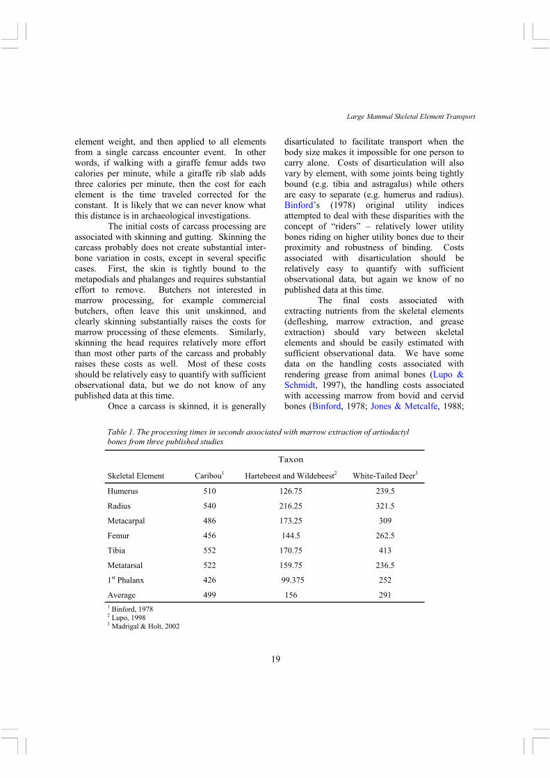
Table 1. The processing times in seconds associated with marrow extraction of artiodactyl bones from three published studies
Taxon
Skeletal Element Caribou1 Hartebeest and Wildebeest2 White-Tailed Deer3
Lupo, 1998; Madrigal & Holt, 2002), and the handling costs associated with meat removal from white-tailed deer (Madrigal & Holt, 2002).
Binford (1978: 26, Table 1.7) provided marrow cavity volume and mean processing time for caribou for all limb bones, mandible, scapula, pelvis, and first and second phalanx. These were then used to calculate a net return expressed as ml/min. Jones and Metcalfe (1988) re-evaluated this data and presented return rate data as calories/hour using a constant of 4 kcal/ml for marrow. Lupo (1998) provided average marrow wet weights and processing time for several impala, wildebeest, hartebeest, and zebra for all the limb bones (1998: 661, Table 2), skull (1998: 662, Table 3), and materials (marrow and fat pad) associated with the first phalanx (1998: 663, Table 4) along with very useful data and discussions about several points of variation in gross yield and return. Lupo provided several variations of gross yield based on different models of health status, as well as net return rates expressed as Kcal/sec (1998: 666, Table 9). Her bovid return rates correlated well with each other, though not all significantly, while her zebra return rates tended to differ markedly from the bovids. Madrigal & Holt (2002) recently provided marrow weights and processing times for the limb bones
and first and second phalanges of white-tailed deer (2002: 751, Table 3), and these were used to construct net return rates as Kcal/hr (2002: 751, Table 4, here expressed as Kcal/sec). Both Lupo and Madrigal & Holt used a constant of 9.37 Kcal/g for marrow yield. It may be pertinent to note that Binford’s data appear to have been recorded under normal butchery circumstances, while both Lupo’s and Madrigal & Holt’s are more experimental in nature in that processing times were recorded under controlled and staged conditions. However, all participants appear to have been skilled at butchery, while only Madrigal & Holt’s hunter did not practice butchery as a subsistence activity –but as a regular sport.
Our main concern here is to compare the consistency between these results, so we will restrict our analysis to those skeletal elements found in each study, and will only use values calculated from adults. With Lupo’s processing time data we have used the average for wildebeest and hartebeest since both are Size 3 (Brain, 1981) animals and overlap in size, and there are only two hartebeest in her sample. However, for her net return rate data we follow her Table 9 and use hartebeest and wildebeest separately. Processing time data are summarized in Table 1, and return
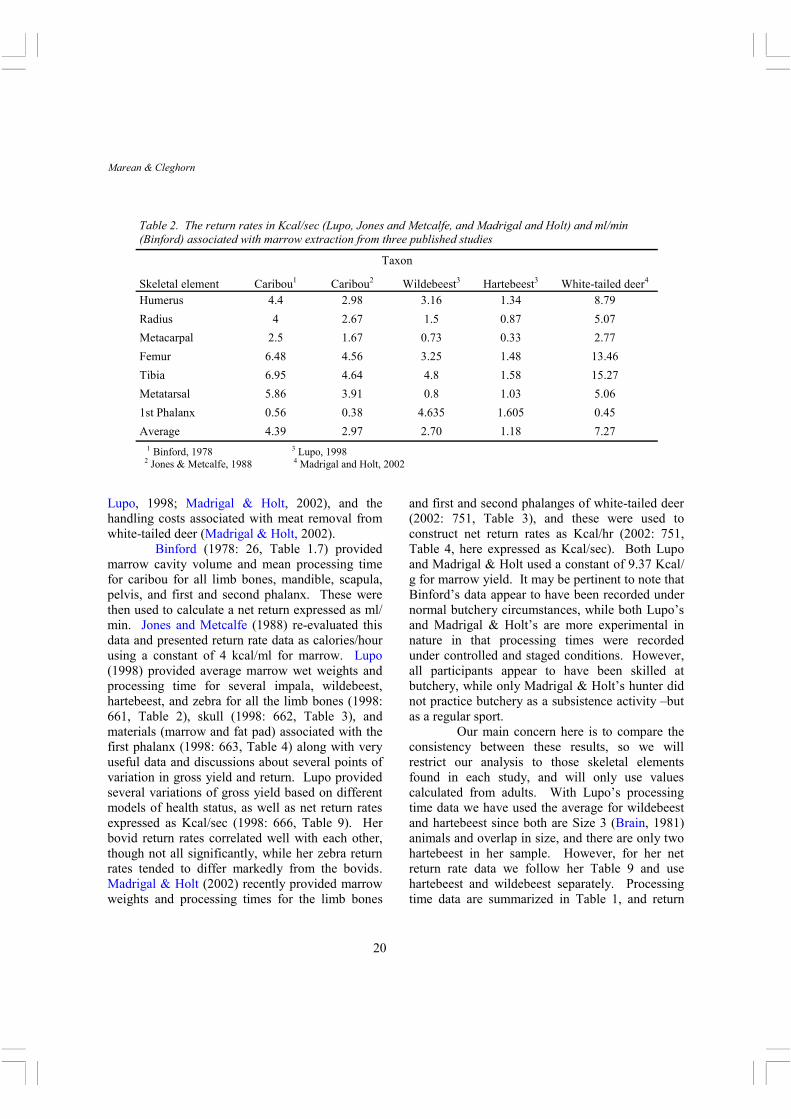
Table 2. The return rates in Kcal/sec (Lupo, Jones and Metcalfe, and Madrigal and Holt) and ml/min (Binford) associated with marrow extraction from three published studies
3 Lupo, 1998
4 Madrigal and Holt, 2002 1 Binford, 1978
2 Jones & Metcalfe, 1988
Skeletal element Caribou1 Caribou2 Wildebeest3 Hartebeest3 White-tailed deer4
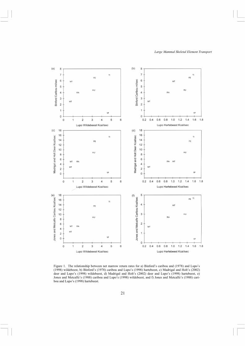
Figure 1. The relationship between net marrow return rates for a) Binford’s caribou and (1978) and Lupo’s (1998) wildebeest, b) Binford’s (1978) caribou and Lupo’s (1998) hartebeest, c) Madrigal and Holt’s (2002) deer and Lupo’s (1998) wildebeest, d) Madrigal and Holt’s (2002) deer and Lupo’s (1998) hartebeest, e) Jones and Metcalfe’s (1988) caribou and Lupo’s (1998) wildebeest, and f) Jones and Metcalfe’s (1988) cari-bou and Lupo’s (1998) hartebeest.
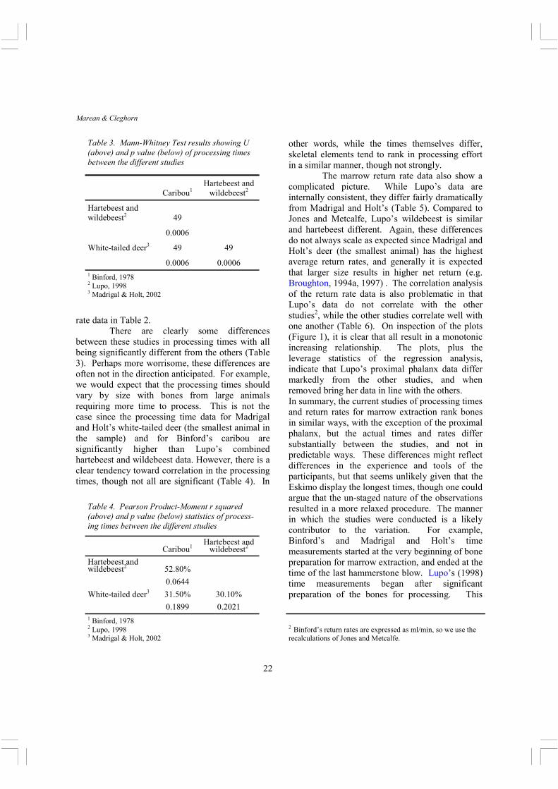
Table 3. Mann-Whitney Test results showing U (above) and p value (below) of processing times between the different studies
rate data in Table 2. There are clearly some differences
between these studies in processing times with all being significantly different from the others (Table 3). Perhaps more worrisome, these differences are often not in the direction anticipated. For example, we would expect that the processing times should vary by size with bones from large animals requiring more time to process. This is not the case since the processing time data for Madrigal and Holt’s white-tailed deer (the smallest animal in the sample) and for Binford’s caribou are significantly higher than Lupo’s combined hartebeest and wildebeest data. However, there is a clear tendency toward correlation in the processing times, though not all are significant (Table 4). In
other words, while the times themselves differ, skeletal elements tend to rank in processing effort in a similar manner, though not strongly.
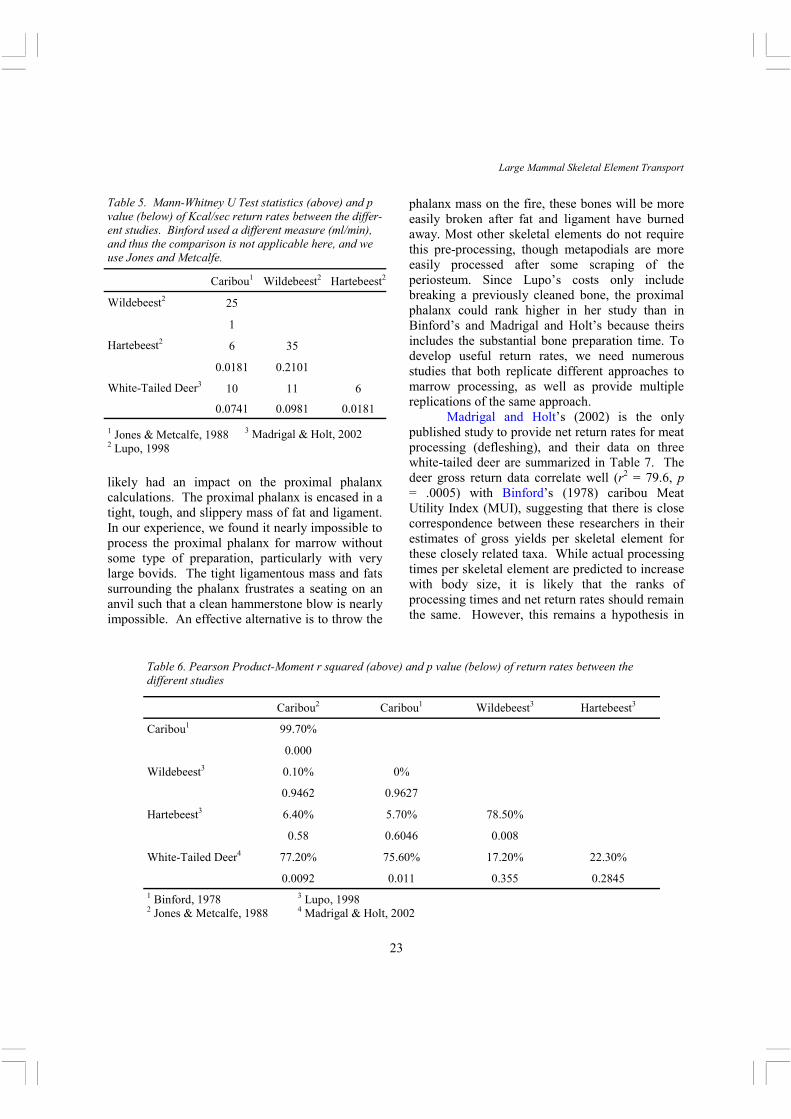
The marrow return rate data also show a complicated picture. While Lupo’s data are internally consistent, they differ fairly dramatically from Madrigal and Holt’s (Table 5). Compared to Jones and Metcalfe, Lupo’s wildebeest is similar and hartebeest different. Again, these differences do not always scale as expected since Madrigal and Holt’s deer (the smallest animal) has the highest average return rates, and generally it is expected that larger size results in higher net return (e.g. Broughton, 1994a, 1997) . The correlation analysis of the return rate data is also problematic in that Lupo’s data do not correlate with the other studies2, while the other studies correlate well with one another (Table 6). On inspection of the plots (Figure 1), it is clear that all result in a monotonic increasing relationship. The plots, plus the leverage statistics of the regression analysis, indicate that Lupo’s proximal phalanx data differ markedly from the other studies, and when removed bring her data in line with the others. In summary, the current studies of processing times and return rates for marrow extraction rank bones in similar ways, with the exception of the proximal phalanx, but the actual times and rates differ substantially between the studies, and not in predictable ways. These differences might reflect differences in the experience and tools of the participants, but that seems unlikely given that the Eskimo display the longest times, though one could argue that the un-staged nature of the observations resulted in a more relaxed procedure. The manner in which the studies were conducted is a likely contributor to the variation. For example, Binford’s and Madrigal and Holt’s time measurements started at the very beginning of bone preparation for marrow extraction, and ended at the time of the last hammerstone blow. Lupo’s (1998) time measurements began after significant preparation of the bones for processing. This
Table 4. Pearson Product-Moment r squared (above) and p value (below) statistics of process-ing times between the different studies
2 Binford’s return rates are expressed as ml/min, so we use the recalculations of Jones and Metcalfe.
23
Large Mammal Skeletal Element Transport
likely had an impact on the proximal phalanx calculations. The proximal phalanx is encased in a tight, tough, and slippery mass of fat and ligament. In our experience, we found it nearly impossible to process the proximal phalanx for marrow without some type of preparation, particularly with very large bovids. The tight ligamentous mass and fats surrounding the phalanx frustrates a seating on an anvil such that a clean hammerstone blow is nearly impossible. An effective alternative is to throw the
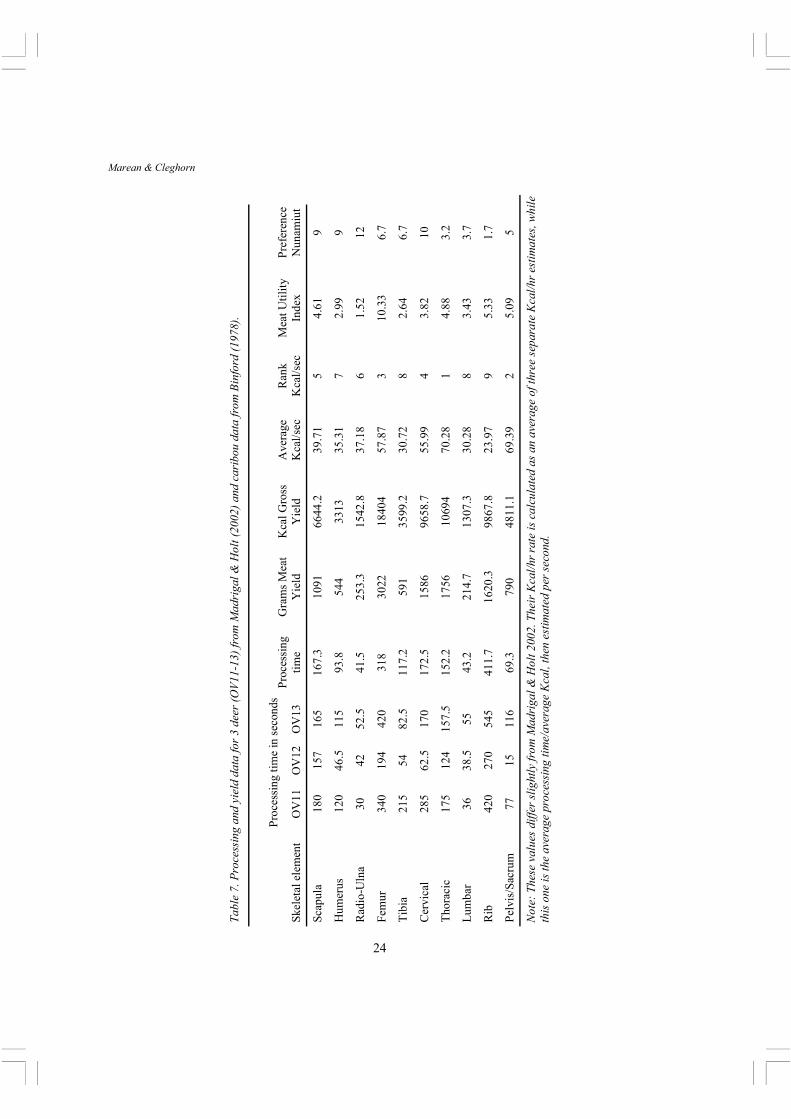
phalanx mass on the fire, these bones will be more easily broken after fat and ligament have burned away. Most other skeletal elements do not require this pre-processing, though metapodials are more easily processed after some scraping of the periosteum. Since Lupo’s costs only include breaking a previously cleaned bone, the proximal phalanx could rank higher in her study than in Binford’s and Madrigal and Holt’s because theirs includes the substantial bone preparation time. To develop useful return rates, we need numerous studies that both replicate different approaches to marrow processing, as well as provide multiple replications of the same approach. Madrigal and Holt’s (2002) is the only published study to provide net return rates for meat processing (defleshing), and their data on three white-tailed deer are summarized in Table 7. The deer gross return data correlate well (r2 = 79.6, p = .0005) with Binford’s (1978) caribou Meat Utility Index (MUI), suggesting that there is close correspondence between these researchers in their estimates of gross yields per skeletal element for these closely related taxa. While actual processing times per skeletal element are predicted to increase with body size, it is likely that the ranks of processing times and net return rates should remain the same. However, this remains a hypothesis in
Table 5. Mann-Whitney U Test statistics (above) and p value (below) of Kcal/sec return rates between the differ-ent studies. Binford used a different measure (ml/min), and thus the comparison is not applicable here, and we use Jones and Metcalfe.
need of testing with further calculations of meat net return rates. Summary of processing costs Grease extraction is the most labor-intensive of the three nutrition-extracting activities, and for people, requires either boiling of the bones (typically fragmented), hanging bones in the sun and catching the grease, or intensive fragmentation followed by ingestion. As Lupo and Schmitt (1997) argue, grease extraction is likely to be practiced only when nutrition is in short supply, or when people have an abundance of protein but lack adequate carbohydrate or fat (see Speth & Spielman, 1983). Marrow extraction is a low cost activity relative to grease extraction in that it only requires a couple of minutes to completely process a bone, particularly if flesh has already been removed. The caloric costs of this activity are minimal since the action includes a low-level of bodily action with small animals, though we note that this increases with the body size of the animal and the thickness of the cortical bone. Importantly, costs associated with marrow extraction do not differ dramatically between bones (on the order of seconds or a few minutes at most). For this reason, we believe it is unlikely that differential marrow processing costs figure strongly in decisions to transport or not. Once transported, there is the decision to marrow process or not. Madrigal and Holt (2002) have argued that if limb bones are processed, then the isolated shafts will survive carnivore ravaging, while non-processed bones will be removed by ravaging carnivores. We agree that this is true. However, they then argue that this process strongly shapes the ultimate skeletal element patterning such that limb bone abundance no longer reflects what was transported, since many bones could be left unprocessed and thus deleted. For this argument to hold, one must argue that even if some limb bones were transported to a site, people would opt to not process them because their return rates were lower than others. Since the caloric cost of processing is so low for any limb bone (particularly once it is prepped by the prior meat removal
process), the difference in processing costs between bones is so low, and the return (of fat) so valuable, that this seems unl ikely. Ethnoarchaeological observations may help to resolve this point. Net vs. gross return rate in ethnoarchaelogical examples Binford (1978) provided justification for the explanatory power of his utility measures in two ways: examining the degree of fit between his utility measures and a measure of Nunamiut food preferences (arrived at by polling nine Nunamiut, Binford, 1978: 41-43), and comparing his gross return rate data with an extensive analysis of SEA at a variety of historic Nunamiut sites. Binford examined the fit between his marrow index and polled Nunamiut marrow bone preference and found a compelling linear relation (1978:43, Figure 1.10). Binford’s marrow index is dominated by the gross return for marrow. Foraging theory posits that foragers should be attempting to maximize net returns, so we should find that net marrow returns correlate even better with Nunamiut preference. However, while all show positive relations between net return and Nunamiut preference, none are significant (Binford’s caribou rs = .086; Lupo’s wildebeest rs = .543 and hartebeest rs = .371; Madrigal and Holt’s deer rs = .543). Given Binford’s success with his marrow index, it would seem that Nunamiut rank marrowbones on gross return, not net.
Madrigal and Holt (2002) have provided the first published net return rate data for defleshing, and there are some interesting patterns revealed. First, the differences in processing time between skeletal elements are not all that dramatic, generally just several minutes. Second, thoracic vertebrae and the pelvis/sacrum unit have the highest return rates, while the return rate of the very meaty femur is dramatically lowered by its relatively high processing times. This high processing time of the femur is inconsistent with our, admittedly anecdotal, experience. It is important to note that Madrigal and Holt (2002)
26
Marean & Cleghorn
Skeletal Element Butchery Cost Femur Low
Sternum Low Tibia Low Rib High
Pelvis/Sacrum High Thoracic High Scapula Low Cervical High Humerus Low Lumbar High
Radius/Ulna Low Phalanges High Mandible High Atlas/Axis High
Skull High Metatarsal Low Metacarpal Low
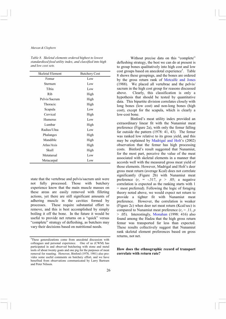
Table 8. Skeletal elements ordered highest to lowest standardized food utility index, and classified into high and low cost sets.
state that the vertebrae and pelvis/sacrum unit were not fully processed. Those with butchery experience know that the main muscle masses on these areas are easily removed with filleting actions, yet there are still significant amounts of adhering muscle in the cavities formed by processes. These require substantial effort to remove, and this is best accomplished by simply boiling it off the bone. In the future it would be useful to provide net returns on a “quick” versus “complete” strategy of defleshing, as butchers may vary their decisions based on nutritional needs.
Without precise data on this “complete” defleshing strategy, the best we can do at present is to group bones qualitatively into high cost and low cost groups based on anecdotal experience3. Table 8 shows these groupings, and the bones are ordered by the gross return rank of Metcalfe and Jones (1988). We placed all vertebrae and the pelvis/sacrum in the high cost group for reasons discussed above. Clearly, this classification is only a hypothesis that should be tested by quantitative data. This bipartite division correlates closely with long bones (low cost) and non-long bones (high cost), except for the scapula, which is clearly a low-cost bone.
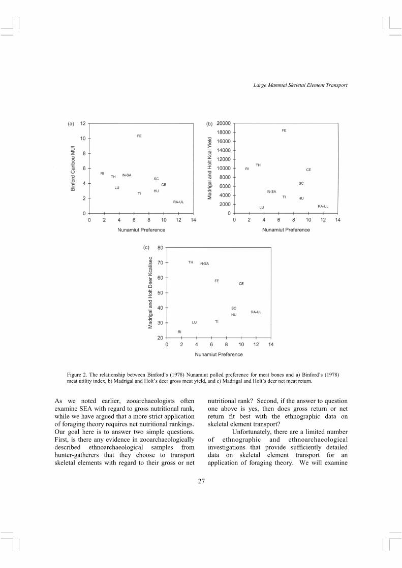
Binford’s meat utility index provided an extraordinary linear fit with the Nunamiut meat preference (Figure 2a), with only the femur falling far outside the pattern (1978: 41, 43). The femur was ranked low relative to its gross yield, and this may be explained by Madrigal and Holt’s (2002) observation that the femur has high processing costs. Binford’s result suggested that Nunamiut, for the most part, perceive the value of the meat associated with skeletal elements in a manner that accords well with the measured gross meat yield of those elements. However, Madrigal and Holt’s deer gross meat return (average Kcal) does not correlate significantly (Figure 2b) with Nunamiut meat preference (rs = -.317, p > .05; a negative correlation is expected as the ranking starts with 1 = most preferred). Following the logic of foraging theory noted above, we would expect net return to provide a tighter fit with Nunamiut meat preference. However, the correlation is weaker (Figure 2c) when deer net meat return (Kcal/sec) is compared to Nunamiut meat preference (rs = .11, p > .05). Interestingly, Monahan (1998: 416) also found among the Hadza that the high gross return femur was transported far less than expected. These results collectively suggest that Nunamiut rank skeletal element preferences based on gross returns, not net.
How does the ethnographic record of transport correlate with return rate?
3These generalizations come from anecdotal discussion with colleagues and personal experience. One of us (CWM) has participated in and observed butchering with stone and metal tools of about twenty goats and one pig for the purposes of meat removal for roasting. However, Binford (1978, 1981) also pro-vides some useful comments on butchery effort, and we have benefited from observations communicated by Larry Bartram and Peter Nilssen.
27
Large Mammal Skeletal Element Transport
Figure 2. The relationship between Binford’s (1978) Nunamiut polled preference for meat bones and a) Binford’s (1978) meat utility index, b) Madrigal and Holt’s deer gross meat yield, and c) Madrigal and Holt’s deer net meat return.
As we noted earlier, zooarchaeologists often examine SEA with regard to gross nutritional rank, while we have argued that a more strict application of foraging theory requires net nutritional rankings. Our goal here is to answer two simple questions. First, is there any evidence in zooarchaeologically described ethnoarchaeological samples from hunter-gatherers that they choose to transport skeletal elements with regard to their gross or net
nutritional rank? Second, if the answer to question one above is yes, then does gross return or net return fit best with the ethnographic data on skeletal element transport?
Unfortunately, there are a limited number of ethnographic and ethnoarchaeological investigations that provide sufficiently detailed data on skeletal element transport for an application of foraging theory. We will examine
28
Marean & Cleghorn
three cases that sample cold, sub-tropical, and tropical environments. The gross skeletal element rankings we will use are derived from Metcalfe and Jones’ (1988) revisions of Binford’s (1978) original data, and we will rely upon their whole bone estimates. We will also use Madrigal and Holt’s (2002) new net return data for white-tailed deer. Only bovids and cervids will be examined and it is assumed that their utility rankings are the same (there is some support for this in Binford, 1978). We will lump bovids and cervids of similar body size into the size groups used by Brain (1981), and assume that utility rankings do not change by size group (again, there is support for this in Emerson, 1990). We will not examine individual cases of carcass butchery and transport, but rather will lump together groups of events. This is consistent with the palimpsest nature of most archaeological assemblages. We will attempt to control for net return rank by employing Madrigal and Holt’s (2002) new data on net returns, though we recognize the potential problems with using white-tailed deer net returns as a proxy for other animals. We will use the high cost/low cost classification previously suggested as a coarse way to model a more complete defleshing scenario.
The Hadza The Hadza, a hunter-gatherer group occupying the arid bushlands and grasslands of the Lake Eyasi basin in northern Tanzania, have recently been the target of study by two different research groups: the Wisconsin group (Bunn, et al. 1988) and the Utah group (Hawkes et al. 1995; Hawkes et al. 1997; O'Connell et al. 1988; O'Connell et al. 1989; O'Connell et al. 1992). The Hadza hunt a variety of large mammals, but their observed hunts are dominated by impala (Size 2), zebra (Size 3), with smaller numbers of hartebeest (Size 3), wildebeest (Size 3), buffalo (Size 4), and eland (Size 4). Monahan (1998) recently synthesized the data from both teams of Hadza researchers, and he argues that there is broad agreement between the results of the two groups. He conducted an analysis of the
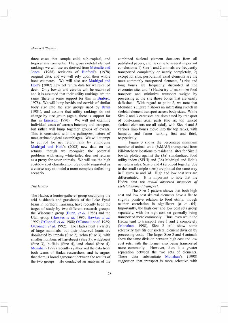
combined skeletal element data-sets from all published papers, and he came to several important conclusions: 1) Size 1 and 2 animals are frequently transported completely or nearly completely, 2) except for ribs, post-cranial axial elements are the most commonly transported elements, 3) ribs and long bones are frequently discarded at the encounter site, and 4) Hadza try to maximize food transport and minimize transport weight by processing at the site those bones that are easily defleshed. With regard to point 2, we note that Monahan’s Figure 5 shows an interesting switch in skeletal element transport across body sizes. While Size 2 and 3 carcasses are dominated by transport of post-cranial axial parts (the six top ranked skeletal elements are all axial), with Size 4 and 5 various limb bones move into the top ranks, with humerus and femur ranking first and third, respectively. Figure 3 shows the percentage minimum number of animal units (%MAU) transported from kill-butchery locations to residential sites for Size 2 bovids plotted against the (3a) standardized food utility index (SFUI) and (3b) Madrigal and Holt’s net return rates. Size 3 and 4 (grouped together due to the small sample sizes) are plotted the same way in Figures 3c and 3d. High and low cost sets are differentiated. It is important to note that the Hadza data are actual observed instances of skeletal element transport.
The Size 2 pattern shows that both high cost and low cost skeletal elements have a flat to slightly positive relation to food utility, though neither correlation is significant (p > .05). Importantly, the high cost and low cost sets group separately, with the high cost set generally being transported more commonly. Thus, even while the Hadza tend to transport Size 1 and 2 completely (Monahan, 1998), Size 2 still show some selectivity that fits our skeletal element division by processing costs. The larger Size 3 and 4 animals show the same division between high cost and low cost sets, with the former also being transported more commonly. However, there is a greater separation between the two sets of elements. These data substantiate Monahan’s (1998) suggestion that transport is more selective with
29
Large Mammal Skeletal Element Transport
larger-bodied animals. When plotted against net return rate, there is virtually no detectable correlation for both Size 2 and combined Sizes 3 and 4 (Figures 3b and 3d, respectively). Overall, these data fail to show any patterning that is similar to the reverse utility curves so common in residential archaeological sites. Conversely, the data fail to show significant positive relations with gross return as measured by
SFUI and net return as estimated by Madrigal and Holt (2002). However, if we accept our division of the skeletal elements into high cost and low cost sets, the data clearly show that the high cost sets are being transported more commonly than the low costs sets, and within the two sets there is a flat relation between utility and transport, suggesting that when a set is transported, it is transported completely. As Monahan (1998) suggests, field
Figure 3. The relationship between Hadza skeletal element transport frequency (in % Minimum Animal Units) of a) Size 2 bovids and Standardized Food Utility, b) Size 2 bovids and Net Meat Return of Madrigal and Holt (2002), c) Size 3 and 4 bovids and Standardized Food Utility, and d) Size 3 and 4 bovids and Net Meat Return of Madrigal and Holt (2002). Solid regression lines apply to High Cost elements, dashed regression lines to Low Cost elements.
30
Marean & Cleghorn
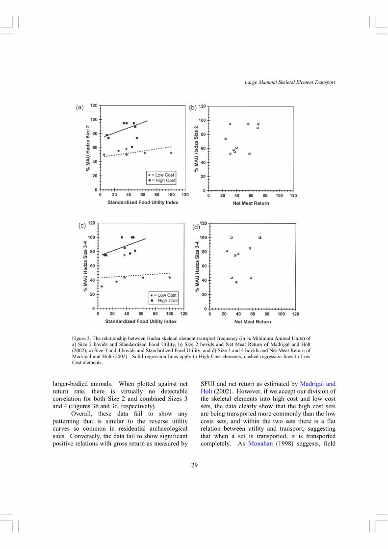
processing of low cost skeletal elements is having a strong impact on the patterning of this data. The Kua Basarwa The Kua are a Khoi-San speaking people inhabiting a semi-arid sub-tropical ecosystem in eastern Botswana (Bartram, 1993, 1997). The Kua hunt a variety of animals that overlap with the Hadza in size range: steenbok (Size 1), bush duiker (Size 1), and gemsbok (Size 3) are their predominant prey. Bartram’s (1993) detailed study of hunting, butchery, and bone transport includes substantial data on SEA in various settings. Unlike the Hadza study, Bartram’s skeletal element data are not observations of transport, but are rather tabulations of skeletal element accumulations that remain at abandoned residential sites. The Kua sites have a short time depth of accumulation and disturbance prior to collection (several days to weeks), but it was reported that hyenas and jackals scavenged from these assemblages before collection and tabulation (Bartram et al., 1991; Bartram, 1993, 1997; Bartram & Marean, 1999). Figure 4 shows the largest sample, the pooled residential sites of Size 3 bovids (mostly
gemsbok), plotted against SFUI and net meat return. Relative to the Hadza, the Kua sample shows no clear distinction between the representations of high and low cost skeletal elements. However, unlike the Hadza, the low cost skeletal elements show a positive but insignificant relation with SFUI (r = .41, p > .05) while the high cost skeletal elements show a negative but insignificant relation with SFUI (r = -.15, p > .05). Clearly, the Hadza pattern of skeletal element transport differs from the Kua pattern of skeletal element representation at abandoned residential sites. Furthermore, the Kua sample shows no correlation with net meat return (Figure 4b).
The Nunamiut Eskimo Binford’s (1978) classic study of the Nunamiut Eskimo, a group of Inuit that focus on caribou (S i ze 3 ) , p rov ides ano the r u se fu l ethnoarchaeological reference. It is important to note that Binford’s (1978) study differs from the Hadza research in that he did not make direct observations on skeletal element transport. Rather, he collected and excavated bones from recent historic sites; sometimes many years after the time
Figure 4. The relationship between Kua skeletal element transport of Size 3 bovids (mostly gemsbok) pooled from all residential sites, relative to a) Standardized Food Utility, and b) Size 2 Net Meat Return of Madrigal and Holt (2002). Solid regression lines apply to High Cost elements, dashed regression lines to Low Cost elements.
31
Large Mammal Skeletal Element Transport
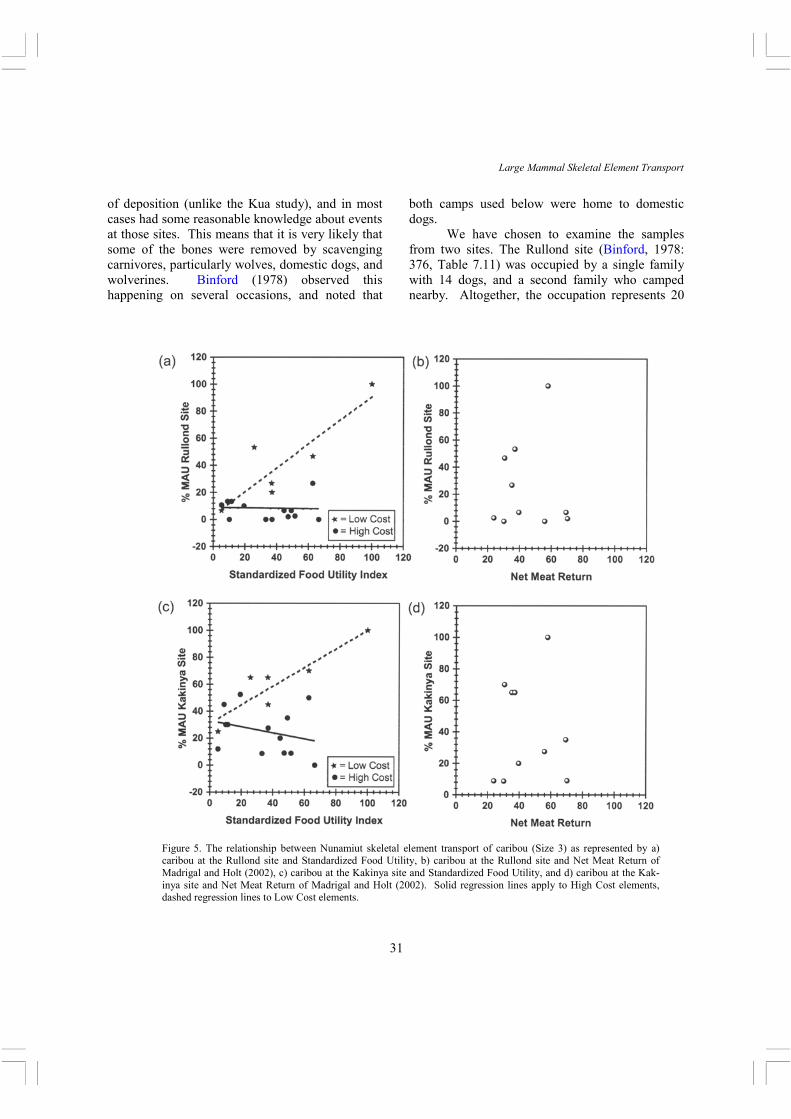
of deposition (unlike the Kua study), and in most cases had some reasonable knowledge about events at those sites. This means that it is very likely that some of the bones were removed by scavenging carnivores, particularly wolves, domestic dogs, and wolverines. Binford (1978) observed this happening on several occasions, and noted that
both camps used below were home to domestic dogs. We have chosen to examine the samples from two sites. The Rullond site (Binford, 1978: 376, Table 7.11) was occupied by a single family with 14 dogs, and a second family who camped nearby. Altogether, the occupation represents 20
Figure 5. The relationship between Nunamiut skeletal element transport of caribou (Size 3) as represented by a) caribou at the Rullond site and Standardized Food Utility, b) caribou at the Rullond site and Net Meat Return of Madrigal and Holt (2002), c) caribou at the Kakinya site and Standardized Food Utility, and d) caribou at the Kak-inya site and Net Meat Return of Madrigal and Holt (2002). Solid regression lines apply to High Cost elements, dashed regression lines to Low Cost elements.
32
Marean & Cleghorn
people for a maximum of 39 days. The site was a favored location from which to make fall hunting sorties on the migrating caribou. The Kakinya site (Binford, 1978: 380-381, Table 7.13) was occupied during the fall migration hunting season by 5 people and 15 dogs. For each site, we use the total SEA. Binford notes that the Kakinya site, unlike the Rullond site, preserved substantial internal structure and included a dog bone yard that is missing from the Rullond site (having been eroded away by meltwater). These two sites were chosen because they are residential sites, and have the largest samples of Binford’s published data. Figure 5 shows caribou SEA at these two sites plotted against SFUI and net meat return. The patterning is very similar between the two sites. The most obvious difference between the Hadza and Nunamiut pattern is that the Nunamiut pattern shows a complete reversal in the representation of high cost and low cost skeletal elements. At both the Rullond and Kakinya sites, low cost elements are more abundant than high cost elements. At the Rullond site, the low cost skeletal elements correlate positively and significantly (r = .79, p < .05) with food utility, while high cost elements correlate negatively but insignificantly (r = -.35, p = .13) with food utility. At the Kakinya Camp, the low cost skeletal elements correlate positively and nearly significantly (r = .78, p = .07) with food utility, while the high cost skeletal elements correlate negatively and nearly significantly (r = -63, p = .09) with food utility. Neither site shows a correlation with net meat return. Interestingly, with the Nunamiut data the high cost set begins to take on the reverse utility pattern so common in archaeological sites. As we argue below, we believe this is due to post-discard destructive processes. Summary of ethnographic cases Overall, these cases show that in the one ethnographic case (the Hadza) where direct observations of skeletal element transport were available for analysis, high cost elements were
transported more commonly than low cost elements. However, within these classifications skeletal elements tended to be transported in equal proportions. Clearly, as Monahan (1998) has argued, and Metcalfe and Barlow’s (1992) discussion indicates, field processing plays a critical role in Hadza skeletal element transport decisions. In the two cases where direct observations of transport were not available (Kua and Nunamiut), and the samples available for analysis were bone accumulations resulting from skeletal element transport and destructive processes, the low cost skeletal elements were present in proportion to their food value while the high cost skeletal elements were not. Not a single sample from any of these ethnographic examples shows a positive correlation with net meat return as recently estimated by Madrigal and Holt (2002). There are at least two potential explanations for the differences seen between these hunter-gatherer groups. First, we could argue that there are clear differences in the way these three groups transport skeletal elements. If this were true, then the Nunamiut would clearly be practicing a low-cost long bone dominated transport strategy, the Kua would be practicing an unbiased strategy where neither high nor low cost skeletal elements were favored, and the Hadza would be practicing a high-cost axial bone dominated transport strategy. Alternatively, the difference between these three samples may result from differences in the timing of data collection relative to deposition and site abandonment. Both the Nunamiut and Kua studies document that carnivores were active at these sites after people discarded the bones. The Hadza observations, by contrast, were made before carnivores had access to the bones. We believe the Kua and Nunamiut pattern can be explained by the well-known tendency for non-long bones to be selectively removed by carnivores from humanly discarded bone assemblages (Bartram & Marean, 1999; Blumenschine & Marean, 1993; Capaldo, 1995; Marean et al., 1992). We believe that these three data-sets represent successive stages in the formation of a faunal assemblage: 1) the Hadza assemblage represents a pristine unmodified faunal collection of transported elements, 2) the Kua data-
33
Large Mammal Skeletal Element Transport
processes of destruction after people have transported and discarded the bones. Here we will distinguish between nutritive and non-nutritive processes of bone destruction. This is a variation on similar ideas by Blumenschine (1986, 1988) and Capaldo (1997). This distinction is important because the nutritive and non-nutritive processes affect bones in different ways. Nutritive processes of destruction are those that result from animals attempting to extract nutrition from the bone and thus are targeted at bone portions where nutrition and bone is not easily separated. Nutrients include marrow within the cortical portions of long bones and mandibles, bone grease that all bovids and cervids store in cancellous bones, and brain matter. Importantly, marrow is separable from cortical bone before consumption, and carnivores typically crack, spit out, ignore, or avoid cortical bone portions (e.g. Binford et al., 1988; Blumenschine & Marean,
set represents an assemblage after several weeks of attrition, and 3) the Nunamiut assemblage represents an assemblage after several months to years of attrition. One of the final stages in the taphonomic history of a skeletal element assemblage is the attrition that occurs in the sediments, as the transported assemblage becomes an archaeological assemblage. This late stage is significant for all archaeological faunal assemblages, as we will see by examining two archaeological cases. But first we develop a basic model that fits the Nunamiut and Kua pattern and can be used to help guide skeletal element applications of foraging theory. A general taphonomic model The primary problem for zooarchaeologists wishing to apply foraging theory principles to SEA is that virtually all faunal assemblages are subject to
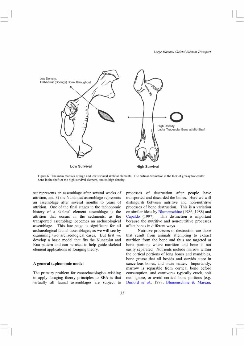
Figure 6. The main features of high and low survival skeletal elements. The critical distinction is the lack of greasy trabecular bone in the shaft of the high survival element, and its high density.
34
Marean & Cleghorn
1993; Blumenschine, 1988; Bunn & Kroll, 1986; Marean & Spencer, 1991). Grease is not mechanically separable from cancellous bone by non-human animals, and thus carnivores chew and swallow the cancellous portions of bone, allowing the digestive tract to render out the grease (e.g. Binford et al., 1988; Blumenschine & Marean, 1993; Blumenschine, 1988; Brain, 1981; Marean & Spencer, 1991). To survive these nutritive processes of destruction and thus be countable to the zooarchaeologist, a bone must have a substantial portion that has thick cortical bone and no cancellous bone (Figure 6). Any bone portion with associated cancellous bone will likely be destroyed or deleted by carnivores scavenging human meals, and we know this process to be geographically and environmentally widespread (Bartram, 1993; Bartram et al., 1991; Bartram & Marean, 1999; Binford, 1978; Binford et al., 1988; Blumenschine, 1988; Bunn, 1991; Capaldo, 1995; 1998; Selvaggio, 1998; Yellen, 1991). A wide variety of taphonomic studies in both naturalistic and experimental conditions, all cited above, have demonstrated the correctness of these generalizations, and it is now safe to say that these statements can be considered a law of site formation process that must guide all zooarchaeological analyses. Non-nutritive processes of bone destruction include those processes that are not the result of animals attempting to derive nutrition. These include trampling, sediment compaction, chemical leaching, burning, and any other chemical or mechanical process that destroys bone. It is widely believed that these processes are density mediated, meaning that the level of destruction is negatively related to the skeletal element’s density (Grayson, 1989; Lyman 1984, 1985, 1992). If this is so, and there is still little experimental research that has documented the relationship between density and survivability in reaction to non-nutritive processes, then there are two important propositions that arise. First, skeletal elements that lack at least some portion that is reasonably dense will rarely survive in an identifiable state. Bone density studies have shown that the densest parts of bovid and cervid skeletons are the thick cortical bone portions of
long bones, and teeth (Kreutzer, 1992; Lam et al., 1998; Lyman, 1984). Second, the only skeletal elements that will record relative abundances that reflect their original discard abundance are those that have similar portions and high density. This discussion leads to three rules that guide the choice of skeletal elements for studies of SEA using principles of foraging theory: 1) The skeletal element must have a substantial portion that has thick cortical bone and lacks cancellous bone (Figure 6). 2) The density through that portion must be high, and the elements chosen for analysis must have similar densities through the cortical portion. 3) That portion must be identifiable to skeletal element, and zooarchaeologists must identify and quantify it accurately. These rules allow us to divide the skeleton into two analytical sets that are useful for investigating different processes. These sets we will call high survival and low survival elements. High survival elements are those that generally fulfill criterion 1 above. This set predominantly overlaps with low cost skeletal elements. These include all of the long bones, mandibles (these basically function like a long bone due to their dense cortical bone and open medullary cavity), and crania (due to the presence of teeth and petrosal). These bones can accurately represent the relative abundance of skeletal elements, and may be usefully investigated using a foraging theory model. The relative representation of low survival (predominantly high cost) elements will reflect their ability to survive the variety of processes that affected the assemblage after its transport and discard. These elements include all vertebrae, ribs, pelves, scapulae (which have thick cortical bone but are difficult to identify and quantify when fragmented), and all tarsals, carpals, and phalanges of Size 1 and 2 animals since these tend to get swallowed by carnivores (Marean, 1991). These elements will be useful for evaluating the level of destruction to which the assemblage has been subjected, and are thus taphonomically but not
35
Large Mammal Skeletal Element Transport
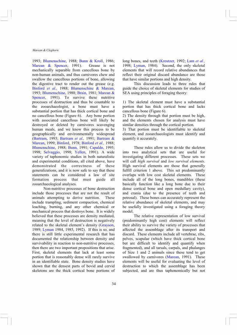
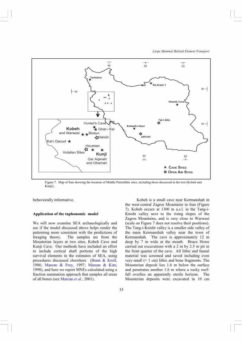
Figure 7. Map of Iran showing the location of Middle Paleolithic sites, including those discussed in the text (Kobeh and Kunji).
behaviorally informative. Application of the taphonomic model We will now examine SEA archaeologically and see if the model discussed above helps render the patterning more consistent with the predictions of foraging theory. The samples are from the Mousterian layers at two sites, Kobeh Cave and Kunji Cave. Our methods have included an effort to include cortical shaft portions of the high survival elements in the estimates of SEA, using procedures discussed elsewhere (Bunn & Kroll, 1986; Marean & Frey, 1997; Marean & Kim, 1998), and here we report MNEs calculated using a fraction summation approach that samples all areas of all bones (see Marean et al., 2001).
Kobeh is a small cave near Kermanshah in the west-central Zagros Mountains in Iran (Figure 7). Kobeh occurs at 1300 m a.s.l. in the Tang-i-Knisht valley next to the rising slopes of the Zagros Mountains, and is very close to Warwasi (scale on Figure 7 does not resolve their positions). The Tang-i-Knisht valley is a smaller side valley of the main Kermanshah valley near the town of Kermanshah. The cave is approximately 12 m deep by 7 m wide at the mouth. Bruce Howe carried out excavations with a 2 m by 2.5 m pit in the front quarter of the cave. All lithic and faunal material was screened and saved including even very small (< 1 cm) lithic and bone fragments. The Mousterian deposit lies 1.6 m below the surface and penetrates another 1.6 m where a rocky roof-fall overlies an apparently sterile horizon. The Mousterian deposits were excavated in 10 cm
36
Marean & Cleghorn
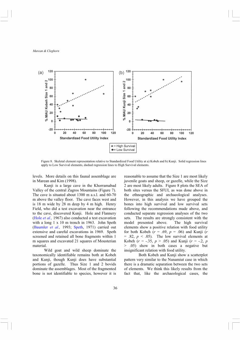
Figure 8. Skeletal element representation relative to Standardized Food Utility at a) Kobeh and b) Kunji. Solid regression lines apply to Low Survival elements, dashed regression lines to High Survival elements.
levels. More details on this faunal assemblage are in Marean and Kim (1998). Kunji is a large cave in the Khorramabad Valley of the central Zagros Mountains (Figure 7). The cave is situated about 1300 m a.s.l. and 60-70 m above the valley floor. The cave faces west and is 18 m wide by 28 m deep by 4 m high. Henry Field, who did a test excavation near the entrance to the cave, discovered Kunji. Hole and Flannery (Hole et al., 1967) also conducted a test excavation with a long 1 x 10 m trench in 1963. John Speth (Baumler et al., 1993; Speth, 1971) carried out extensive and careful excavations in 1969. Speth screened and retained all bone fragments within 1 m squares and excavated 21 squares of Mousterian material. Wild goat and wild sheep dominate the taxonomically identifiable remains both at Kobeh and Kunji, though Kunji does have substantial portions of gazelle. Thus Size 1 and 2 bovids dominate the assemblages. Most of the fragmented bone is not identifiable to species, however it is
reasonable to assume that the Size 1 are most likely juvenile goats and sheep, or gazelle, while the Size 2 are most likely adults. Figure 8 plots the SEA of both sites versus the SFUI, as was done above in the ethnographic and archaeological analyses. However, in this analysis we have grouped the bones into high survival and low survival sets following the recommendations made above, and conducted separate regression analyses of the two sets. The results are strongly consistent with the model presented above. The high survival elements show a positive relation with food utility for both Kobeh (r = .69, p = .06) and Kunji (r = .82, p < .05). The low survival elements at Kobeh (r = -.35, p > .05) and Kunji (r = -.2, p > .05) show in both cases a negative but insignificant relation with food utility.
Both Kobeh and Kunji show a scatterplot pattern very similar to the Nunamiut case in which there is a dramatic separation between the two sets of elements. We think this likely results from the fact that, like the archaeological cases, the
37
Large Mammal Skeletal Element Transport
Nunamiut skeletal elements have undergone significant nutritive destruction from carnivores, thereby lowering the abundance of the low survival skeletal elements (the high cost set). The Kobeh and Kunji cases represent a final stage of deletion of low survival-high cost elements beyond that observed with the Nunamiut data, where their abundance is a function of various post-nutritive processes of bone destruction as well. The positive and significant correlations between the high survival set and food utility are consistent with what we would expect hunter-gatherers to do, given our results from the ethnographic cases: those elements are being transported in a manner consistent with their gross returns. Summary and conclusions In the prior discussion we provided a distinction between high cost and low cost skeletal elements in an attempt to control for the impact of complete processing costs on skeletal elements. We found that in the ethnographic case where actual observations of transport are available, the high cost elements were transported more frequently than the low cost elements. Monahan (1998) has argued that this results from decisions on the part of the Hadza to shed bone weight prior to transport if it can be done easily. However, this pattern was not evident in the Kua data-set, and the precise opposite of this pattern was found with the Nunamiut data-sets. We argued that this reversal in pattern is likely to represent post-discard attrition of the faunal assemblages, resulting in depressed relative representation of the high cost skeletal elements. The new net return rate data provided by Madrigal and Holt (2002) did not correlate well with any of the ethnographic data, suggesting that transport decisions may be governed more by a strategy focused on maximizing gross returns while minimizing weight. However, there are some important factors effecting net return that have not been thoroughly studied, and future research may result in different results. We then summarized a wide range of
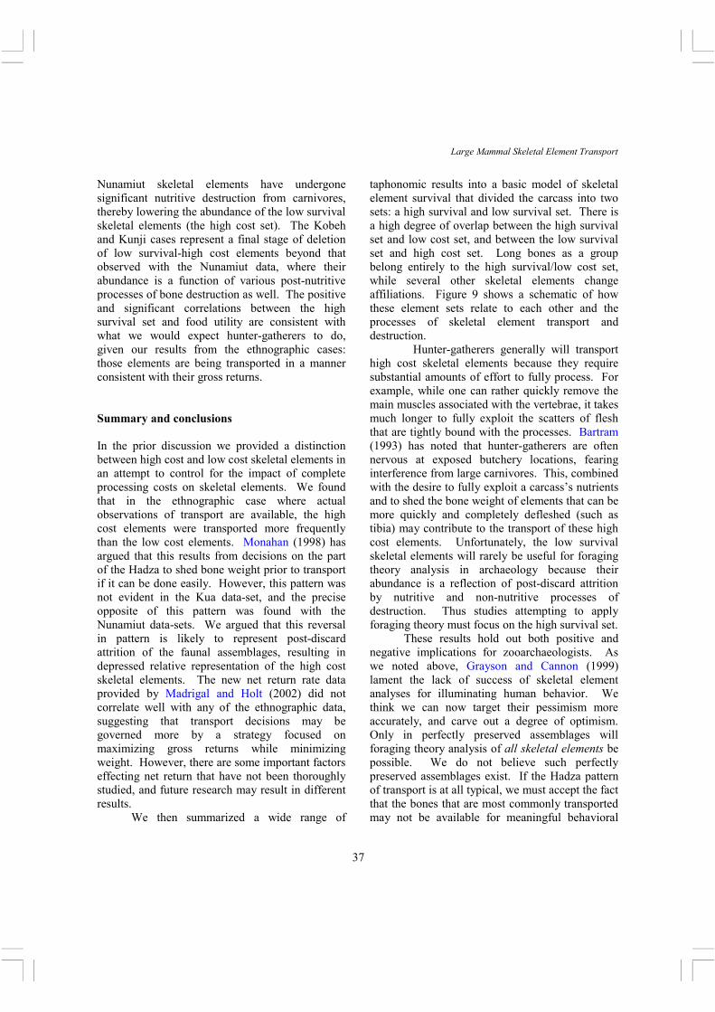
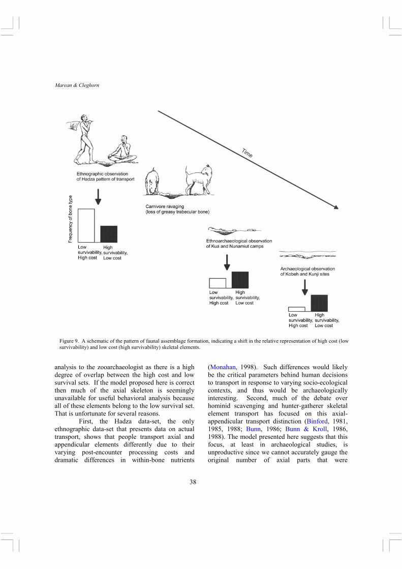
taphonomic results into a basic model of skeletal element survival that divided the carcass into two sets: a high survival and low survival set. There is a high degree of overlap between the high survival set and low cost set, and between the low survival set and high cost set. Long bones as a group belong entirely to the high survival/low cost set, while several other skeletal elements change affiliations. Figure 9 shows a schematic of how these element sets relate to each other and the processes of skeletal element transport and destruction.
Hunter-gatherers generally will transport high cost skeletal elements because they require substantial amounts of effort to fully process. For example, while one can rather quickly remove the main muscles associated with the vertebrae, it takes much longer to fully exploit the scatters of flesh that are tightly bound with the processes. Bartram (1993) has noted that hunter-gatherers are often nervous at exposed butchery locations, fearing interference from large carnivores. This, combined with the desire to fully exploit a carcass’s nutrients and to shed the bone weight of elements that can be more quickly and completely defleshed (such as tibia) may contribute to the transport of these high cost elements. Unfortunately, the low survival skeletal elements will rarely be useful for foraging theory analysis in archaeology because their abundance is a reflection of post-discard attrition by nutritive and non-nutritive processes of destruction. Thus studies attempting to apply foraging theory must focus on the high survival set. These results hold out both positive and negative implications for zooarchaeologists. As we noted above, Grayson and Cannon (1999) lament the lack of success of skeletal element analyses for illuminating human behavior. We think we can now target their pessimism more accurately, and carve out a degree of optimism. Only in perfectly preserved assemblages will foraging theory analysis of all skeletal elements be possible. We do not believe such perfectly preserved assemblages exist. If the Hadza pattern of transport is at all typical, we must accept the fact that the bones that are most commonly transported may not be available for meaningful behavioral
38
Marean & Cleghorn
Figure 9. A schematic of the pattern of faunal assemblage formation, indicating a shift in the relative representation of high cost (low survivability) and low cost (high survivability) skeletal elements.
analysis to the zooarchaeologist as there is a high degree of overlap between the high cost and low survival sets. If the model proposed here is correct then much of the axial skeleton is seemingly unavailable for useful behavioral analysis because all of these elements belong to the low survival set. That is unfortunate for several reasons.
First, the Hadza data-set, the only ethnographic data-set that presents data on actual transport, shows that people transport axial and appendicular elements differently due to their varying post-encounter processing costs and dramatic differences in within-bone nutrients
(Monahan, 1998). Such differences would likely be the critical parameters behind human decisions to transport in response to varying socio-ecological contexts, and thus would be archaeologically interesting. Second, much of the debate over hominid scavenging and hunter-gatherer skeletal element transport has focused on this axial-appendicular transport distinction (Binford, 1981, 1985, 1988; Bunn, 1986; Bunn & Kroll, 1986, 1988). The model presented here suggests that this focus, at least in archaeological studies, is unproductive since we cannot accurately gauge the original number of axial parts that were
39
Large Mammal Skeletal Element Transport
transported. On the positive side, the high survival elements can be the basis for investigations of SEA guided by foraging theory. However, the Hadza data suggest that these are transported on average secondary to most of the bones of the axial skeleton. Thus our archaeological view on skeletal element transport is biased toward those bones that are often not the highest ranked for transport. We still need to address a final question. Is this high survival set sufficiently diverse and behaviorally sensitive to allow us to ask interesting foraging theory questions? The answer to this question lies in the ethnographic data-sets on skeletal element transport. These old data-sets, and any new ones that can still be generated, need to be examined by archaeologists from the perspective of what is archaeologically useful - the high survival elements. It is important to note that the high survival set proposed here includes bones from both the limb region and skull and it is very likely that these two regions are transported very differently in response to different socio-ecological contexts. Also, within the limb the upper long bones (humerus-radius and femur-tibia) are significant meat-bearing bones while the metapodials are not. Careful examination of the relative representation of these bones may reveal interesting behavioral patterns. O’Connell (1995) recently argued that actualistic study was in a theoretical crisis in that it had no guiding general theory, and he proposed behavioral ecology as a useful focus. While we certainly agree with this, that point cuts both ways: robust applications of general theory require strong middle range theory, particularly in archaeological applications where the unit of observation is not human action, but rather the discarded remnants of human action. That extra inferential step forces constraints on the application of behavioral ecological principles, and those constraints surround the question of whether our unit of measurement is measuring human behavior, or some other taphonomic process. Our model argues that the entire skeleton is likely unavailable for productive analysis, but that we can productively apply behavioral ecological analyses to the high survival set. This result, grounded in middle range
research, has obvious practical applications. But more generally, it shows that general theory is helpless without a tight link to the middle range theory that has been developed by years of incremental, and perhaps outwardly rather empirical, taphonomic research. Acknowledgements Marean thanks Tom Minichillo and Mike Cannon for inviting him to participate in their symposium at the 1999 SAA’s from which this paper grew. The analysis of the faunal collections was funded by NSF grant SBR-9727668 to Marean. We thank James Garza for the illustration in Figure 9, and Travis Pickering for his productive input and careful editing. References Bartram, L.E. (1993). An ethnoarchaeological analysis of Kua
San (Botswana) bone food refuse. Unpublished Ph.D. dissertation, University of Wisconsin, Madison.
Bartram, L.E. (1997). A comparison of Kua (Botswana) and Hadza (Tanzania) bow and arrow hunting. In (H. Knecht, Ed.) Projectile Technology. Plenum Press: New York and London, pp. 321-343.
Bartram, L.E., Kroll, E.M., & Bunn, H.T. (1991). Variability in camp structure and bone food refuse patterning at Kua San hunter-gatherer camps. In (E.M. Kroll & T. Douglas, Ed.) The Interpretation of Archaeological Spatial Patterning. Plenum Press: New York, pp. 77-148.
Bartram, L. & Marean, C.W. (1999). Explaining the "Klasies Pattern": Kua ethnoarchaeology, the Die Kelders Middle Stone Age archaeofauna, long bone fragmentation and carnivore ravaging. Journal of Archaeological Science, 26: 9-29.
Baumler, M.F. & Speth, J.D. (1993). A Middle Paleolithic assemblage from Kunji Cave, Iran. In (D.I. Olszewski & H.L. Dibble, Ed.) The Paleolithic Prehistory of the Zagros-Taurus. The University Museum of Archaeology and Anthropology, University of Pennsylvania: Philadelphia, pp. 1-74.
Binford, L.R. (1978). Nunamiut Ethnoarchaeology. Academic Press: New York.
Binford, L.R. (1981). Bones: Ancient Men and Modern Myths. Academic Press: New York.
Binford, L.R. (1984). The faunal remains from Klasies River Mouth. Academic Press: New York
Binford, L.R. (1985). Human ancestors: changing views of their behavior. Journal of Anthropological Archaeology, 4: 292-327.
40
Marean & Cleghorn
Binford, L.R. (1988). Fact and fiction about the Zinjanthropus floor: Data, arguments, and interpretations. Current Anthropology, 29: 123-135.
Binford, L.R., Mills, L.G.L. & Stone, N.M. (1988). Hyena scavenging behavior and its implications for the interpretation of faunal assemblages from FLK 22 (the Zinj floor) at Olduvai Gorge. Journal of Anthropological Archaeology, 7: 99-135.
Blumenschine, R.J. (1986). Carcass consumption sequences and the archaeological distinction of scavenging and hunting. Journal of Human Evolution, 15: 639-659.
Blumenschine, R.J. (1988). An experimental model of the timing of hominid and carnivore influence on archaeological bone assemblages. Journal of Archaeological Science, 15: 483-502.
Blumenschine, R.J. & Caro , T. (1986). Unit flesh weights of some East African bovids. African Journal of Ecology, 24: 273-286.
Blumenschine, R.J. & Madrigal, T.C. (1993). Variability in long bone marrow yields of East African Ungulates and its zooarchaeological implications. Journal of Archaeological Science, 24: 555-587.
Blumenschine, R.J. & Marean, C.W. (1993). A carnivore's view of archaeological bone assemblages. In (J. Hudson, Ed.) From Bones to Behavior. Center for Archaeological Investigations: Carbondale, pp. 273-301.
Brain, C.K. (1981). The Hunters or the Hunted? University of Chicago Press: Chicago.
Brink, J.& Dawe, B. (1989). Final Report of the 1985 and 1986 Field Season at Head-Smashed-in Buffalo Jump, Alberta. Archaeological Survey of Alberta: Edmonton.
Broughton, J.M. (1994a). Declines in mammalian foraging efficiency during the late Holocene, San Francisco Bay, California. Journal of Anthropological Archaeology, 13: 371-401.
Broughton, J.M. (1994b). Late Holocene resource intensification in the Sacramento Valley, California: The vertebrate evidence. Journal of Archaeological Science, 21: 501-514.
Broughton, J.M. (1998). Widening diet breadth, declining foraging efficiency, and prehistoric harvest pressure: Ichthyofaunal evidence from the Emeryville Shellmound, California. Antiquity, 71: 845-862.
Broughton, J. M. & Grayson, D. K. (1993). Diet breadth, adaptive change, and the White Mountains faunas. Journal of Archaeological Science, 20: 331-336.
Bunn, H.T. (1986). Patterns of skeletal element representation and hominid subsistence activities at Olduvai Gorge, Tanzania, and Koobi Fora, Kenya. Journal of Human Evolution, 15: 673-690.
Bunn, H. T. (1991). A taphonomic perspective on the archaeology of human origins. Annual Review of Anthropology, 20: 433-467.
Bunn, H.T., Bartram, L.E. & Kroll, E.M. (1988). Variability in bone assemblage formation from Hadza hunting, scavenging, and carcass processing. Journal of Anthropological Archaeology, 7: 412-457.
Bunn, H.T. & Kroll, E.M. (1986). Systematic butchery by Plio-Pleistocene hominids at Olduvai Gorge, Tanzania.
Current Anthropology, 27: 431-452. Bunn, H.T. & Kroll, E.M. (1988). Fact and fiction about the
Zinjanthropus floor: Data, arguments, and interpretations. Current Anthropology, 29: 135-149.
Capaldo, S.D. (1995). Inferring hominid and carnivore behavior from dual-patterned archaeofaunal assemblages. Unpublished Ph.D. dissertation, Rutgers University: New Brunswick.
Capaldo, S.D. (1997). Experimental determinations of carcass processing by Plio-Pleistocene hominids and carnivores at FLK 22 (Zinjanthropus), Olduvai Gorge, Tanzania. Journal of Human Evolution, 33: 555-597.
Capaldo, S.D. (1998). Simulating the formation of dual-patterned archaeofaunal assemblages with experimental control samples. Journal of Archaeological Science, 25: 311-330.
Emerson, A.M. (1990). Archaeological Implications of Variability in the Economic Anatomy of Bison bison. Unpublished Ph.D. dissertation, Washington State University: Pullman.
Grayson, D.K. (1989). Bone transport, bone destruction, and reverse utility curves. Journal of Archaeological Science, 16: 643-652.
Grayson, D. K. (1991). Alpine faunas from the White Mountains, California: adaptive change in the Late Prehistoric Great Basin? Journal of Archaeological Science, 18: 483-506.
Grayson, D. K. (2001). The archaeological record of human impacts on animal populations. Journal of World Prehistory, 15: 1-68.
Grayson, D. K. & Delpech, F. (1998). Changing diet breadth in the Early Upper Palaeolithic of southwestern France. Journal of Archaeological Science, 25: 1119-1129.
Grayson, D. K. & Cannon, M. D. (1999). Human paleoecology and foraging theory in the Great Basin. In (C. Beck, Ed.) Models for the Millennium: Great Basin Anthropology Today. University of Utah Press: Salt Lake City, pp. 141-151.
Grayson, D. K., Delpech, F., Rigaud, J.-P., & Simek, J. F. (2001). Explaining the development of dietary dominance by a single ungulate taxon at Grotte XVI, Dordogne, France. Journal of Archaeological Science, 28: 115-125.
Hawkes, K., O'Connell, J.F. & Blurton-Jones, N.G. (1995). Hadza children's foraging: juvenile dependency, social arrangements, and mobility among hunter-gatherers. Current Anthropology, 36: 688-700.
Hawkes, K., O'Connell, J.F. & Blurton-Jones, N.G. (1997).Hadza women's time allocation, offspring provisioning, and the evolution of long postmenopausal life spans. Current Anthropology, 38: 551-577.
Hole, F. & Flannery, K. (1967). The prehistory of south-western Iran: a preliminary report. Proceedings of the Prehistoric Society, 33: 151-206.
Jones, K.T. & Metcalfe, D. (1988). Bare bones archaeology: bone marrow indices and efficiency. Journal of Archaeological Science, 15: 415-423.
Krebs, J.R. & Davies, N.B. (1981). An Introduction to Behavioural Ecology. Blackwell Scientific Publications: Boston.
41
Large Mammal Skeletal Element Transport
Kreutzer, L.A. (1992). Bison and deer bone mineral densities: Comparisons and implications for the interpretation of archaeological fauna. Journal of Archaeological Science, 19: 271-294.
Lam, Y.M., Chen, X., Marean, C.W. & Frey, C.J. (1998). Bone density and long bone representation in archaeological faunas: comparing results from CT and photon densitometry. Journal of Archaeological Science, 25: 559-570.
Lupo, K.D. (1998).Experimentally derived extraction rates for marrow: implications for body part exploitation strategies of Plio-Pleistocene Hominid scavengers. Journal of Archaeological Science, 25: 657-676.
Lupo, K.D. & Schmitt, D.N. (1997). Experiments in bone boiling: nutritional returns and archaeological reflections. Anthropozoologica, 25-26: 137-144.
Lyman, R.L. (1984). Bone density and differential survivorship of fossil classes. Journal of Anthropological Archaeology, 3: 259-299.
Lyman, R.L. (1985). Bone frequencies: Differential transport, in situ destruction, and the MGUI. Journal of Archaeological Science, 12: 221-236.
Lyman, R.L. (1992). Anatomical considerations of utility curves in zooarchaeology. Journal of Archaeological Science, 19: 7-22.
Madrigal, T. C. & Holt, J. Z. (2002). White-tailed deer meat and marrow return rates and their application to Eastern Woodlands archaeology. American Antiquity, 67: 745-759.
Marean, C.W. (1991). Measuring the postdepositional destruction of bone in archaeological assemblages. Journal of Archaeological Science, 18: 677-694.
Marean, C.W. (1992). Hunter to herder: Large mammal remains from the hunter-gatherer occupation at Enkapune Ya Muto rockshelter (Central Rift, Kenya). African Archaeological Review, 10: 65-127.
Marean, C. W., Abe, Y., Nilssen, P. J., & Stone, E. C. (2001). Estimating the minimum number of skeletal elements (MNE) in zooarchaeology: a review and a new image-analysis GIS approach. American Antiquity, 66: 333-348.
Marean, C.W. & Assefa, Z. (1999). Zooarchaeological evidence for the faunal exploitation behavior of Neandertals and Early Modern Humans. Evolutionary Anthropology, 7: 22-37.
Marean, C.W. & Frey, C.J. (1997). The animal bones from caves to cities: reverse utility curves as methodological artifacts. American Antiquity, 62: 698-711.
Marean, C.W. & Kim, S.Y. (1998). Mousterian faunal remains from Kobeh cave (Zagros Mountains, Iran): behavioral implications for Neanderthals and early modern humans. Current Anthropology, 39: S79-S114.
Marean, C.W. & Spencer, L.M. (1991). Impact of carnivore ravaging on zooarchaeological measures of element abundance. American Antiquity, 56: 645-658.
Marean, C.W., Spencer, L.M., Blumenschine, R.J. & Capaldo, R.J. (1992). Captive hyena bone choice and destruction, the schlepp effect, and Olduvai archaeofaunas. Journal of Archaeological Science, 19: 101-121.
Metcalfe, D. & Barlow, K.R. (1992). A model for exploring the optimal trade-off between field processing and transport. American Anthropologist, 94: 340-356.
Metcalfe, D. & Jones, K.T. (1988). A reconsideration of animal
body-part utility indices. American Antiquity, 53: 486-504. Monahan, C.M. (1998). The Hadza carcass transport debate
revisited and its archaeological implications. Journal of Archaeological Science, 25: 405-424.
O'Connell, J.F. (1995). Ethnoarchaeology needs a general theory of behavior. Journal of Archaeological Research, 3: 205-255.
O'Connell, J.F. & Hawkes, K. (1988). Hadza hunting, butchering, and bone transport and their archaeological implications. Journal of Anthropological Research, 44: 113-161.
O'Connell, J.F., Hawkes, K. & Blurton-Jones, N. (1988). Hadza scavenging: implications for Plio-Pleistocene hominid subsistence. Current Anthropology, 29: 356-363.
O'Connell, J.F., Hawkes, K. & Blurton-Jones, N. (1989). Reanalysis of large mammal body part transport among the Hadza. Journal of Archaeological Science, 17: 301-316.
O'Connell, J.F., Hawkes, K. & Blurton-Jones, N. (1992). Patterns in the distribution, site structure and assemblage composition of Hadza kill-butchering sites. Journal of Archaeological Science, 19: 319-345.
Raab, L.M. (1992). An optimal foraging analysis of prehistoric shellfish collecting on San Clemente island, California. Journal of Ethnobiology, 12: 63-80.
Selvaggio, M.M. (1998). Evidence for a three-stage sequence of hominid and carnivore involvement with long bones at FLK Zinjanthropus, Olduvai Gorge, Tanzania. Journal of Archaeological Science, 25: 191-202.
Sih, A. & Christensen, B. (2001). Optimal diet theory: when does it work, and when and why does it fail? Animal Behavior, 61: 379-390.
Speth, J.D. (1971). Kunji Cave. Iran, 9:172-173. Speth, J.D. (1983). Bison Kills and Bone Counts. University of
Chicago Press: Chicago. Speth, J.D. (1987). Early hominid subsistence strategies in
seasonal habitats. Journal of Archaeological Science, 14: 13-29.
Speth, J.D. & Spielman, K.A. (1983). Energy source, protein metabolism, and hunter-gatherer subsistence strategies. Journal of Anthropological Archaeology, 2: 1-31.
Stephens, D. & Krebs, J. (1986). Foraging Theory. Princeton University Press: Princeton.
Stiner, M. C., Munro, N. D., & Surovell, T. A. (2000). The tortoise and the hare: small-game use, the broad-spectrum revolution, and Paleolithic demography. Current Anthropology, 41: 39-73.
Stiner, M. C., Munro, N. D., Surovell, T. A., Tchernov, E., & Bar-Yosef, O. (1999). Paleolithic population growth pulses evidenced by small animal exploitation. Science, 283: 190-194.
Thomas, D.H. & Mayer, D. (1983). Behavioral faunal analysis of selected horizons. In (D.H. Thomas, Ed.). The Archaeology of Monitor Valley 2: Gatecliff Shelter, American Museum of Natural History: New York, pp. 353-391.
White, T. E. (1952). Observations on the butchering technique of some aboriginal peoples, No.1. American Antiquity, 17: 337-338.
White, T. E. (1953). Observations on the butchering technique
42
Marean & Cleghorn
of some aboriginal peoples, No. 2. American Antiquity, 19: 160-164.
White, T. E. (1954). Observations on the butchering technique of some aboriginal peoples, Nos.3, 4, 5, and 6. American Antiquity, 20: 254-264.
White, T. E. (1955). Observations on the butchering techniques of some aboriginal peoples numbers 7, 8, and 9 American Antiquity, 21: 170-178.
Yellen, J.E. (1991). Small mammals: !Kung San utilization and production of faunal assemblages. Journal of Anthropological Archaeology, 10: 1-26.