arXiv:1805.00909v3 [cs.LG] 20 May 2018 Reinforcement Learning and Control as Probabilistic Inference: Tutorial and Review Sergey Levine UC Berkeley [email protected]Abstract The framework of reinforcement learning or optimal control provides a mathe- matical formalization of intelligent decision making that is powerful and broadly applicable. While the general form of the reinforcement learning problem enables effective reasoning about uncertainty, the connection between reinforcement learn- ing and inference in probabilistic models is not immediately obvious. However, such a connection has considerable value when it comes to algorithm design: for- malizing a problem as probabilistic inference in principle allows us to bring to bear a wide array of approximate inference tools, extend the model in flexible and powerful ways, and reason about compositionality and partial observability. In this article, we will discuss how a generalization of the reinforcement learning or optimal control problem, which is sometimes termed maximum entropy rein- forcement learning, is equivalent to exact probabilistic inference in the case of deterministic dynamics, and variational inference in the case of stochastic dynam- ics. We will present a detailed derivation of this framework, overview prior work that has drawn on this and related ideas to propose new reinforcement learning and control algorithms, and describe perspectives on future research. 1 Introduction Probabilistic graphical models (PGMs) offer a broadly applicable and useful toolbox for the machine learning researcher (Koller and Friedman, 2009): by couching the entirety of the learning problem in the parlance of probability theory, they provide a consistent and flexible framework to devise prin- cipled objectives, set up models that reflect the causal structure in the world, and allow a common set of inference methods to be deployed against a broad range of problem domains. Indeed, if a particular learning problem can be set up as a probabilistic graphical model, this can often serve as the first and most important step to solving it. Crucially, in the framework of PGMs, it is sufficient to write down the model and pose the question, and the objectives for learning and inference emerge automatically. Conventionally, decision making problems formalized as reinforcement learning or optimal control have been cast into a framework that aims to generalize probabilistic models by augmenting them with utilities or rewards, where the reward function is viewed as an extrinsic signal. In this view, determining an optimal course of action (a plan) or an optimal decision-making strategy (a policy) is a fundamentally distinct type of problem than probabilistic inference, although the underlying dynamical system might still be described by a probabilistic graphical model. In this article, we instead derive an alterate view of decision making, reinforcement learning, and optimal control, where the decision making problem is simply an inference problem in a particular type of graphical model. Formalizing decision making as inference in probabilistic graphical models can in principle allow us to to bring to bear a wide array of approximate inference tools, extend the model in flexible and powerful ways, and reason about compositionality and partial observability. Specifically, we will discuss how a generalization of the reinforcement learning or optimal control problem, which is sometimes termed maximum entropy reinforcement learning, is equivalent to ex- act probabilistic inference in the case of deterministic dynamics, and variational inference in the case of stochastic dynamics. This observation is not a new one, and the connection between proba- bilistic inference and control has been explored in the literature under a variety of names, including
Transcript
arX
iv:1
805.
0090
9v3
[cs
.LG
] 2
0 M
ay 2
018
Reinforcement Learning and Control as Probabilistic
The framework of reinforcement learning or optimal control provides a mathe-matical formalization of intelligent decision making that is powerful and broadlyapplicable. While the general form of the reinforcement learning problem enableseffective reasoning about uncertainty, the connection between reinforcement learn-ing and inference in probabilistic models is not immediately obvious. However,such a connection has considerable value when it comes to algorithm design: for-malizing a problem as probabilistic inference in principle allows us to bring tobear a wide array of approximate inference tools, extend the model in flexible andpowerful ways, and reason about compositionality and partial observability. Inthis article, we will discuss how a generalization of the reinforcement learningor optimal control problem, which is sometimes termed maximum entropy rein-forcement learning, is equivalent to exact probabilistic inference in the case ofdeterministic dynamics, and variational inference in the case of stochastic dynam-ics. We will present a detailed derivation of this framework, overview prior workthat has drawn on this and related ideas to propose new reinforcement learningand control algorithms, and describe perspectives on future research.
1 Introduction
Probabilistic graphical models (PGMs) offer a broadly applicable and useful toolbox for the machinelearning researcher (Koller and Friedman, 2009): by couching the entirety of the learning problemin the parlance of probability theory, they provide a consistent and flexible framework to devise prin-cipled objectives, set up models that reflect the causal structure in the world, and allow a commonset of inference methods to be deployed against a broad range of problem domains. Indeed, if aparticular learning problem can be set up as a probabilistic graphical model, this can often serve asthe first and most important step to solving it. Crucially, in the framework of PGMs, it is sufficientto write down the model and pose the question, and the objectives for learning and inference emergeautomatically.
Conventionally, decision making problems formalized as reinforcement learning or optimal controlhave been cast into a framework that aims to generalize probabilistic models by augmenting themwith utilities or rewards, where the reward function is viewed as an extrinsic signal. In this view,determining an optimal course of action (a plan) or an optimal decision-making strategy (a policy)is a fundamentally distinct type of problem than probabilistic inference, although the underlyingdynamical system might still be described by a probabilistic graphical model. In this article, weinstead derive an alterate view of decision making, reinforcement learning, and optimal control,where the decision making problem is simply an inference problem in a particular type of graphicalmodel. Formalizing decision making as inference in probabilistic graphical models can in principleallow us to to bring to bear a wide array of approximate inference tools, extend the model in flexibleand powerful ways, and reason about compositionality and partial observability.
Specifically, we will discuss how a generalization of the reinforcement learning or optimal controlproblem, which is sometimes termed maximum entropy reinforcement learning, is equivalent to ex-act probabilistic inference in the case of deterministic dynamics, and variational inference in thecase of stochastic dynamics. This observation is not a new one, and the connection between proba-bilistic inference and control has been explored in the literature under a variety of names, including
the Kalman duality (Todorov, 2008), maximum entropy reinforcement learning (Ziebart, 2010), KL-divergence control (Kappen et al., 2012; Kappen, 2011), and stochastic optimal control (Toussaint,2009). While the specific derivations the differ, the basic underlying framework and optimizationobjective are the same. All of these methods involve formulating control or reinforcement learningas a PGM, either explicitly or implicitly, and then deploying learning and inference methods fromthe PGM literature to solve the resulting inference and learning problems.
Formulating reinforcement learning and decision making as inference provides a number of otherappealing tools: a natural exploration strategy based on entropy maximization, effective tools forinverse reinforcement learning, and the ability to deploy powerful approximate inference algorithmsto solve reinforcement learning problems. Furthermore, the connection between probabilistic infer-ence and control provides an appealing probabilistic interpretation for the meaning of the rewardfunction, and its effect on the optimal policy. The design of reward or cost functions in reinforce-ment learning is oftentimes as much art as science, and the choice of reward often blurs the linebetween algorithm and objective, with task-specific heuristics and task objectives combined into asingle reward. In the control as inference framework, the reward induces a distribution over randomvariables, and the optimal policy aims to explicitly match a probability distribution defined by thereward and system dynamics, which may in future work suggest a way to systematize reward design.
This article will present the probabilistic model that can be used to embed a maximum entropy gener-alization of control or reinforcement learning into the framework of PGMs, describe how to performinference in this model – exactly in the case of deterministic dynamics, or via structured variationalinference in the case of stochastic dynamics, – and discuss how approximate methods based onfunction approximation fit within this framework. Although the particular variational inference in-terpretation of control differs somewhat from the presentation in prior work, the goal of this article isnot to propose a fundamentally novel way of viewing the connection between control and inference.Rather, it is to provide a unified treatment of the topic in a self-contained and accessible tutorial for-mat, and to connect this framework to recent research in reinforcement learning, including recentlyproposed deep reinforcement learning algorithms. In addition, this article presents a review of therecent reinforcement learning literature that relates to this view of control as probabilistic inference,and offers some perspectives on future research directions.
The basic graphical model for control will be presented in Section 2, variational inference forstochastic dynamics will be discussed in Section 3, approximate methods based on function ap-proximation, including deep reinforcement learning, will be discussed in Section 4, and a surveyand review of recent literature will be presented in Section 5. Finally, we will discuss perspectiveson future research directions in Section 6.
2 A Graphical Model for Control as Inference
In this section, we will present the basic graphical model that allows us to embed control into theframework of PGMs, and discuss how this framework can be used to derive variants of severalstandard reinforcement learning and dynamic programming approaches. The PGM presented in thissection corresponds to a generalization of the standard reinforcement learning problem, where theRL objective is augmented with an entropy term. The magnitude of the reward function trades offbetween reward maximization and entropy maximization, allowing the original RL problem to berecovered in the limit of infinitely large rewards. We will begin by defining notation, then definingthe graphical model, and then presenting several inference methods and describing how they relate tostandard algorithms in reinforcement learning and dynamic programming. Finally, we will discussa few limitations of this method and motivate the variational approach in Section 3.
2.1 The Decision Making Problem and Terminology
First, we will introduce the notation we will use for the standard optimal control or reinforcementlearning formulation. We will use s ∈ S to denote states and a ∈ A to denote actions, which mayeach be discrete or continuous. States evolve according to the stochastic dynamics p(st+1|st, at),which are in general unknown. We will follow a discrete-time finite-horizon derivation, with horizonT , and omit discount factors for now. A discount γ can be readily incorporated into this frameworksimply by modifying the transition dynamics, such that any action produces a transition into anabsorbing state with probability 1 − γ, and all standard transition probabilities are multiplied by γ.
2
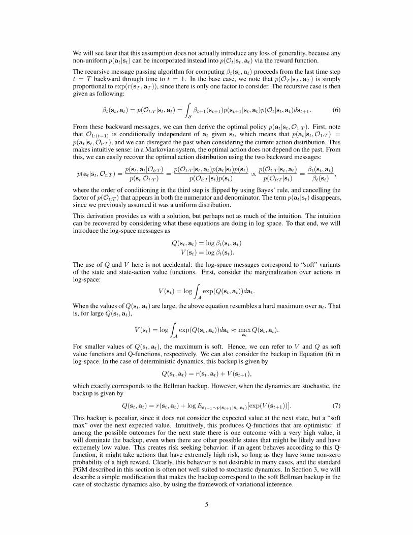
a1 a2 a3 a4
s1 s2 s3 s4
(a) graphical model with states and actions
a1 a2 a3 a4
s1 s2 s3 s4
O1 O2 O3 O4
(b) graphical model with optimality variables
Figure 1: The graphical model for control as inference. We begin by laying out the states and actions, whichform the backbone of the model (a). In order to embed a control problem into this model, we need to addnodes that depend on the reward (b). These “optimality variables” correspond to observations in a HMM-style framework: we condition on the optimality variables being true, and then infer the most probable actionsequence or most probable action distributions.
A task in this framework can be defined by a reward function r(st, at). Solving a task typicallyinvolves recovering a policy p(at|st, θ), which specifies a distribution over actions conditioned onthe state parameterized by some parameter vector θ. A standard reinforcement learning policy searchproblem is then given by the following maximization:
θ⋆ = argmaxθ
T∑
t=1
E(st,at)∼p(st,at|θ)[r(st, at)]. (1)
This optimization problem aims to find a vector of policy parameters θ that maximize the totalexpected reward
∑
t r(st, at) of the policy. The expectation is taken under the policy’s trajectorydistribution p(τ), given by
p(τ) = p(s1, at, . . . , sT , aT |θ) = p(s1)
T∏
t=1
p(at|st, θ)p(st+1|st, at). (2)
For conciseness, it is common to denote the action conditional p(at|st, θ) as πθ(at|st), to emphasizethat it is given by a parameterized policy with parameters θ. These parameters might correspond,for example, to the weights in a neural network. However, we could just as well embed a standardplanning problem in this formulation, by letting θ denote a sequence of actions in an open-loop plan.
Having formulated the decision making problem in this way, the next question we have to ask toderive the control as inference framework is: how can we formulate a probabilistic graphical modelsuch that the most probable trajectory corresponds to the trajectory from the optimal policy? Or,equivalently, how can we formulate a probabilistic graphical model such that inferring the posterioraction conditional p(at|st, θ) gives us the optimal policy?
2.2 The Graphical Model
To embed the control problem into a graphical model, we can begin simply by modeling the rela-tionship between states, actions, and next states. This relationship is simple, and corresponds to agraphical model with factors of the form p(st+1|st, at), as shown in Figure 1 (a). However, thisgraphical model is insufficient for solving control problems, because it has no notion of rewards orcosts. We therefore have to introduce an additional variable into this model, which we will denoteOt. This additional variable is a binary random variable, where Ot = 1 denotes that time step t isoptimal, andOt = 0 denotes that it is not optimal. We will choose the distribution over this variableto be given by the following equation:
p(Ot = 1|st, at) = exp(r(st, at)). (3)
The graphical model with these additional variables is summarized in Figure 1 (b). While this mightat first seem like a peculiar and arbitrary choice, it leads to a very natural posterior distribution over
3
actions when we condition onOt = 1 for all t ∈ {1, . . . , T }:
p(τ |o1:T ) ∝ p(τ,o1:T ) = p(s1)
T∏
t=1
p(Ot = 1|st, at)p(st+1|st, at)
= p(s1)
T∏
t=1
exp(r(st, at))p(st+1|st, at)
=
[
p(s1)T∏
t=1
p(st+1|st, at)
]
exp
(
T∑
t=1
r(st, at)
)
. (4)
That is, the probability of observing a given trajectory is given by the product between its probabilityto occur according to the dynamics (the term in square brackets on the last line), and the exponentialof the total reward along that trajectory. It is most straightforward to understand this equation insystems with deterministic dynamics, where the first term is a constant for all trajectories that aredynamically feasible. In this case, the trajectory with the highest reward has the highest probability,and trajectories with lower reward have exponentially lower probability. If we would like to planfor an optimal action sequence starting from some initial state s1, we can condition on o1:T andchoose p(s1) = δ(s1), in which case maximum a posteriori inference corresponds to a kind ofplanning problem. It is easy to see that this exactly corresponds to standard planning or trajectoryoptimization in the case where the dynamics are deterministic, in which case Equation (4) reducesto
p(τ |o1:T ) ∝ 1[p(τ) 6= 0] exp
(
T∑
t=1
r(st, at)
)
. (5)
Here, the indicator function simply indicates that the trajectory τ is dynamically consistent (meaningthat p(st+1|st, at) 6= 0) and the initial state is correct. The case of stochastic dynamics poses somechallenges, and will be discussed in detail in Section 3. However, even under deterministic dynamics,we are often interested in recovering a policy rather than a plan. In this PGM, the optimal policycan be written as p(at|st,Ot:T = 1) (we will drop = 1 in the remainder of the derivation forconciseness). This distribution is somewhat analogous to p(at|st, θ
⋆) in the previous section, withtwo major differences: first, it is independent of the parameterization θ, and second, we will seelater that it optimizes an objective that is slightly different from the standard reinforcement learningobjective in Equation (1).
2.3 Policy Search as Probabilistic Inference
We can recover the optimal policy p(at|st,Ot:T ) using a standard sum-product inference algorithm,analogously to inference in HMM-style dynamic Bayesian networks. As we will see in this section,it is sufficient to compute backward messages of the form
βt(st, at) = p(Ot:T |st, at).
These messages have a natural interpretation: they denote the probability that a trajectory can beoptimal for time steps from t to T if it begins in state st with the action at.
1 Slightly overloadingthe notation, we will also introduce the message
βt(st) = p(Ot:T |st).
These messages denote the probability that the trajectory from t to T is optimal if it begins in state st.We can recover the state-only message from the state-action message by integrating out the action:
βt(st) = p(Ot:T |st) =
∫
A
p(Ot:T |st, at)p(at|st)dat =
∫
A
βt(st, at)p(at|st)dat.
The factor p(at|st) is the action prior. Note that it is not conditioned on O1:T in any way: it doesnot denote the probability of an optimal action, but simply the prior probability of actions. ThePGM in Figure 1 doesn’t actually contain this factor, and we can assume that p(at|st) = 1
|A| for
simplicity – that is, it is a constant corresponding to a uniform distribution over the set of actions.
1Note that βt(st,at) is not a probability density over st,at, but rather the probability of Ot:T = 1.
4
We will see later that this assumption does not actually introduce any loss of generality, because anynon-uniform p(at|st) can be incorporated instead into p(Ot|st, at) via the reward function.
The recursive message passing algorithm for computing βt(st, at) proceeds from the last time stept = T backward through time to t = 1. In the base case, we note that p(OT |sT , aT ) is simplyproportional to exp(r(sT , aT )), since there is only one factor to consider. The recursive case is thengiven as following:
βt(st, at) = p(Ot:T |st, at) =
∫
S
βt+1(st+1)p(st+1|st, at)p(Ot|st, at)dst+1. (6)
From these backward messages, we can then derive the optimal policy p(at|st,O1:T ). First, notethat O1:(t−1) is conditionally independent of at given st, which means that p(at|st,O1:T ) =p(at|st,Ot:T ), and we can disregard the past when considering the current action distribution. Thismakes intuitive sense: in a Markovian system, the optimal action does not depend on the past. Fromthis, we can easily recover the optimal action distribution using the two backward messages:
p(at|st,Ot:T ) =p(st, at|Ot:T )
p(st|Ot:T )=p(Ot:T |st, at)p(at|st)p(st)
p(Ot:T |st)p(st)∝p(Ot:T |st, at)
p(Ot:T |st)=βt(st, at)
βt(st),
where the order of conditioning in the third step is flipped by using Bayes’ rule, and cancelling thefactor of p(Ot:T ) that appears in both the numerator and denominator. The term p(at|st) disappears,since we previously assumed it was a uniform distribution.
This derivation provides us with a solution, but perhaps not as much of the intuition. The intuitioncan be recovered by considering what these equations are doing in log space. To that end, we willintroduce the log-space messages as
Q(st, at) = log βt(st, at)
V (st) = log βt(st).
The use of Q and V here is not accidental: the log-space messages correspond to “soft” variantsof the state and state-action value functions. First, consider the marginalization over actions inlog-space:
V (st) = log
∫
A
exp(Q(st, at))dat.
When the values ofQ(st, at) are large, the above equation resembles a hard maximum over at. Thatis, for large Q(st, at),
V (st) = log
∫
A
exp(Q(st, at))dat ≈ maxat
Q(st, at).
For smaller values of Q(st, at), the maximum is soft. Hence, we can refer to V and Q as softvalue functions and Q-functions, respectively. We can also consider the backup in Equation (6) inlog-space. In the case of deterministic dynamics, this backup is given by
Q(st, at) = r(st, at) + V (st+1),
which exactly corresponds to the Bellman backup. However, when the dynamics are stochastic, thebackup is given by
This backup is peculiar, since it does not consider the expected value at the next state, but a “softmax” over the next expected value. Intuitively, this produces Q-functions that are optimistic: ifamong the possible outcomes for the next state there is one outcome with a very high value, itwill dominate the backup, even when there are other possible states that might be likely and haveextremely low value. This creates risk seeking behavior: if an agent behaves according to this Q-function, it might take actions that have extremely high risk, so long as they have some non-zeroprobability of a high reward. Clearly, this behavior is not desirable in many cases, and the standardPGM described in this section is often not well suited to stochastic dynamics. In Section 3, we willdescribe a simple modification that makes the backup correspond to the soft Bellman backup in thecase of stochastic dynamics also, by using the framework of variational inference.
5
2.4 Which Objective does This Inference Procedure Optimize?
In the previous section, we derived an inference procedure that can be used to obtain the distributionover actions conditioned on all of the optimality variables, p(at|st,O1:T ). But which objective doesthis policy actually optimize? Recall that the overall distribution is given by
p(τ) =
[
p(s1)
T∏
t=1
p(st+1|st, at)
]
exp
(
T∑
t=1
r(st, at)
)
, (8)
which we can simplify in the case of deterministic dynamics into Equation (5). In this case, theconditional distributions p(at|st,O1:T ) are simply obtained by marginalizing the full trajectory dis-tribution and conditioning the policy at each time step on st. We can adopt an optimization-basedapproximate inference approach to this problem, in which case the goal is to fit an approximationπ(at|st) such that the trajectory distribution
p(τ) ∝ 1[p(τ) 6= 0]
T∏
t=1
π(at|st)
matches the distribution in Equation (5). In the case of exact inference, as derived in the previous sec-tion, the match is exact, which means that DKL(p(τ)‖p(τ)) = 0, where DKL is the KL-divergence.We can therefore view the inference process as minimizing DKL(p(τ)‖p(τ)), which is given by
DKL(p(τ)‖p(τ)) = −Eτ∼p(τ)[log p(τ)− log p(τ)].
Negating both sides and substituting in the equations for p(τ) and p(τ), we get
Therefore, minimizing the KL-divergence corresponds to maximizing the expected reward and theexpected conditional entropy, in contrast to the standard control objective in Equation (1), whichonly maximizes reward. Hence, this type of control objective is sometimes referred to as maximumentropy reinforcement learning or maximum entropy control.
However, that in the case of stochastic dynamics, the solution is not quite so simple. Under stochasticdynamics, the optimized distribution is given by
p(τ) = p(s1|O1:T )
T∏
t=1
p(st+1|st, at,O1:T )p(at|st,O1:T ), (9)
where the initial state distribution and the dynamics are also conditioned on optimality. As a resultof this, the dynamics and initial state terms in the KL-divergence do not cancel, and the objectivedoes not have the simple entropy maximizing form derived above.2 We can still fall back on theoriginal KL-divergence minimization at the trajectory level, and write the objective as
−DKL(p(τ)‖p(τ)) = Eτ∼p(τ)
[
log p(s1) +
T∑
t=1
r(st, at) + log p(st+1|st, at)
]
+H(p(τ)). (10)
2In the deterministic case, we know that p(st+1|st,at,O1:T ) = p(st+1|st, at), since exactly one transitionis ever possible.
6
However, because of the log p(st+1|st, at) terms, this objective is difficult to optimize in a model-free setting. As discussed in the previous section, it also results in an optimistic policy that assumes adegree of control over the dynamics that is unrealistic in most control problems. In Section 3, we willderive a variational inference procedure that does reduce to the convenient objective in Equation (9)even in the case of stochastic dynamics, and in the process also addresses the risk-seeking behaviordiscussed in Section 2.3.
2.5 Alternative Model Formulations
It’s worth pointing out that the definition of p(Ot = 1|st, at) in Equation (3) requires an additionalassumption, which is that the rewards r(st, at) are always negative.3 Otherwise, we end up with anegative probability for p(Ot = 0|st, at). However, this assumption is not actually required: it’squite possible to instead define the graphical model with an undirected factor on (st, at,Ot), with anunnormalized potential given by Φt(st, at,Ot) = 1Ot=1 exp(r(st, at)). The potential for Ot = 0doesn’t matter, since we always condition on Ot = 1. This leads to the same exact inference proce-dure as the one we described above, but without the negative reward assumption. Once we are con-tent to working with undirected graphical models, we can even remove the variablesOt completely,and simply add an undirected factor on (st, at) with the potential Φt(st, at) = exp(r(st, at)),which is mathematically equivalent. This is the conditional random field formulation describedby Ziebart (Ziebart, 2010). The analysis and inference methods in this model are identical to theones for the directed model with explicit optimality variablesOt, and the particular choice of modelis simply a notational convenience. We will use the variables Ot in this article for clarity of deriva-tion and stay within the directed graphical model framework, but all derivations are straightforwardto reproduce in the conditional random field formulation.
Another common modification to this framework is to incorporate an explicit temperature α into theCPD for Ot, such that p(Ot|st, bat) = exp( 1
αr(st, at)). The corresponding maximum entropy ob-
jective can then be written equivalently as the expectation of the (original) reward, with an additionalmultiplier of α on the entropy term. This provides a natural mechanism to interpolate between en-tropy maximization and standard optimal control or RL: as α→ 0, the optimal solution approachesthe standard optimal control solution. Note that this does not actually increase the generality of themethod, since the constant 1
αcan always be multiplied into the reward, but making this temperature
constant explicit can help to illuminate the connection between standard and entropy maximizingoptimal control.
Finally, it is worth remarking again on the role of discount factors: it is very common in reinforce-ment learning to use a Bellman backup of the form
where γ ∈ (0, 1] is a discount factor. This allows for learning value functions in infinite-horizonsettings, where the backup would otherwise be non-convergent for γ = 1, and reduces variancefor Monte Carlo advantage estimators in policy gradient algorithms (Schulman et al., 2016). Thediscount factor can be viewed a simple redefinition of the system dynamics. If the initial dynamicsare given by p(st+1|st, at), adding a discount factor is equivalent to undiscounted value fitting underthe modified dynamics p(st+1|st, at) = γp(st+1|st, at), where there is an additional transition withprobability 1 − γ, regardless of action, into an absorbing state with reward zero. We will omit γfrom the derivations in this article, but it can be inserted trivially in all cases simply by modifyingthe (soft) Bellman backups in any place where the expectation over p(st+1|st, at) occurs, such asEquation (7) previously or Equation (15) in the next section.
3 Variational Inference and Stochastic Dynamics
The problematic nature of the maximum entropy framework in the case of stochastic dynamics, dis-cussed in Section 2.3 and Section 2.4, in essence amounts to an assumption that the agent is allowedto control both its actions and the dynamics of the system in order to produce optimal trajectories,but its authority over the dynamics is penalized based on deviation from the true dynamics. Hence,the log p(st+1|st, at) terms in Equation (10) can be factored out of the equations, producing additive
3This assumption is not actually very strong: if we assume the reward is bounded above, we can alwaysconstruct an exactly equivalent reward simply by subtracting the maximum reward.
7
terms that corresponds to the cross-entropy between the posterior dynamics p(st+1|st, at,O1:T ) andthe true dynamics p(st+1|st, at). This explains the risk-seeking nature of the method discussed inSection 2.3: if the agent is allowed to influence its dynamics, even a little bit, it would reasonablychoose to remove unlikely but extremely bad outcomes of risky actions.
Of course, in practical reinforcement learning and control problems, such manipulation of systemdynamics is not possible, and the resulting policies can lead to disastrously bad outcomes. We cancorrect this issue by modifying the inference procedure. In this section, we will derive this correctionby freezing the system dynamics, writing down the corresponding maximum entropy objective, andderiving a dynamic programming procedure for optimizing it. Then we will show that this procedureamounts to a direct application of structured variational inference.
3.1 Maximum Entropy Reinforcement Learning with Fixed Dynamics
The issue discussed in Section 2.4 for stochastic dynamics can briefly be summarized as following:since the posterior dynamics distribution p(st+1|st, at,O1:T ) does not necessarily match the truedynamics p(st+1|st, at), the agent assumes that it can influence the dynamics to a limited extent.A simple fix to this issue is to explicitly disallow this control, by forcing the posterior dynamicsand initial state distributions to match p(st+1|st, at) and p(s1), respectively. Then, the optimizedtrajectory distribution is given simply by
p(τ) = p(s1)
T∏
t=1
p(st+1|st, at)π(at|st),
and the same derivation as the one presented in Section 2.4 for the deterministic case results in thefollowing objective:
−DKL(p(τ)‖p(τ)) =
T∑
t=1
E(st,at)∼p(st,at))[r(st, at) +H(π(at|st))]. (11)
That is, the objective is still to maximize reward and entropy, but now under stochastic transitiondynamics. To optimize this objective, we can compute backward messages like we did in Section 2.3.However, since we are now starting from the maximization of the objective in Equation (11), we haveto derive these backward messages from an optimization perspective as a dynamic programmingalgorithm. As before, we will begin with the base case of optimizing π(aT |sT ), which maximizes
where the equality holds from the definition of KL-divergence, and exp(V (sT )) is the normalizingconstant for exp(r(sT , aT )) with respect to aT where V (sT ) = log
∫
A exp(r(sT , aT ))daT , whichis the same soft maximization as in Section 2.3. Since we know that the KL-divergence is minimizedwhen the two arguments represent the same distribution, the optimal policy is given by
π(aT |sT ) = exp (r(sT , aT )− V (sT )) , (13)
The recursive case can then computed as following: for a given time step t, π(at|st) must maximizetwo terms:
The first term follows directly from the objective in Equation (11), while the second term representsthe contribution of π(at|st) to the expectations of all subsequent time steps. The second term de-serves a more in-depth derivation. First, consider the base case: given the equation for π(aT |sT )in Equation (13), we can evaluate the objective for the policy by directly substituting this equationinto Equation (12). Since the KL-divergence then evaluates to zero, we are left only with the V (sT )term. In the recursive case, we note that we can rewrite the objective in Equation (14) as
which corresponds to a standard Bellman backup with a soft maximization for the value function.Choosing
π(at|st) = exp (Q(st, at)− V (st)) , (16)
we again see that the KL-divergence evaluates to zero, leaving Est∼p(st)[V (st)] as the only remain-
ing term in the objective for time step t, just like in the base case of t = T . This means that, if we fixthe dynamics and initial state distribution, and only allow the policy to change, we recover a Bellmanbackup operator that uses the expected value of the next state, rather than the optimistic estimate wesaw in Section 2.3 (compare Equation (15) to Equation (7)). While this provides a solution to thepractical problem of risk-seeking policies, it is perhaps a bit unsatisfying in its divergence from theconvenient framework of probabilistic graphical models. In the next section, we will discuss howthis procedure amounts to a direct application of structured variational inference.
3.2 Connection to Structured Variational Inference
One way to interpret the optimization procedure in Section 3.1 is as a particular type of structuredvariational inference. In structured variational inference, our goal is to approximate some distribu-tion p(y) with another, potentially simpler distribution q(y). Typically, q(y) is taken to be sometractable factorized distribution, such as a product of conditional distributions connected in a chainor tree, which lends itself to tractable exact inference. In our case, we aim to approximate p(τ),given by
p(τ) =
[
p(s1)T∏
t=1
p(st+1|st, at)
]
exp
(
T∑
t=1
r(st, at)
)
, (17)
via the distribution
q(τ) = q(s1)
T∏
t=1
q(st+1|st, at)q(at|st). (18)
If we fix q(s1) = p(s1) and q(st+1|st, at) = p(st+1|st, at), then q(τ) is exactly the distributionp(τ) from Section 3.1, which we’ve renamed here to q(τ) to emphasize the connection to structuredvariational inference. Note that we’ve also renamed π(at|st) to q(at|st) for the same reason. Instructured variational inference, approximate inference is performed by optimizing the variationallower bound (also called the evidence lower bound). Recall that our evidence here is that Ot = 1for all t ∈ {1, . . . , T }, and the posterior is conditioned on the initial state s1. The variational lowerbound is given by
where the inequality on the last line is obtained via Jensen’s inequality. Substituting the definitionsof p(τ) and q(τ) from Equations (17) and (18), and noting the cancellation due to q(st+1|st, at) =p(st+1|st, at), the bound reduces to
log p(O1:T ) ≥ E(s1:T ,a1:T )∼q(s1:T ,a1:T )
[
T∑
t=1
r(st, at)− log q(at|st)
]
, (19)
up to an additive constant. Optimizing this objective with respect to the policy q(at|st) correspondsexactly to the objective in Equation (11). Intuitively, this means that this objective attempts to find
9
the closest match to the maximum entropy trajectory distribution, subject to the constraint that theagent is only allowed to modify the policy, and not the dynamics. Note that this framework canalso easily accommodate any other structural constraints on the policy, including restriction to aparticular distribution class (e.g., conditional Gaussian, or a categorical distribution parameterizedby a neural network), or restriction to partial observability, where the entire state st is not availableas an input, but rather the policy only has access to some non-invertible function of the state.
4 Approximate Inference with Function Approximation
We saw in the discussion above that a dynamic programming backward algorithm with updates thatresemble Bellman backups can recover “soft” analogues of the value function and Q-function inthe maximum entropy reinforcement learning framework, and the stochastic optimal policy can berecovered from the Q-function and value function. In this section, we will discuss how practical al-gorithms for high-dimensional or continuous reinforcement learning problems can be derived fromthis theoretical framework, with the use of function approximation. This will give rise to several pro-totypical methods that mirror corresponding techniques in standard reinforcement learning: policygradients, actor-critic algorithms, and Q-learning.
4.1 Maximum Entropy Policy Gradients
One approach to performing structured variational inference is to directly optimize the evidencelower bound with respect to the variational distribution (Koller and Friedman, 2009). This approachcan be directly applied to maximum entropy reinforcement learning. Note that the variational distri-bution consists of three terms: q(s1), q(st+1|st, at), and q(at|st). The first two terms are fixed top(s1) and p(st+1|st, at), respectively, leaving only q(at|st) to vary. We can parameterize this distri-bution with any expressive conditional, with parameters θ, and will therefore denote it as qθ(at|st).The parameters could correspond, for example, to the weights in a deep neural network, which takesst as input and outputs the parameters of some distribution class. In the case of discrete actions, thenetwork could directly output the parameters of a categorical distribution (e.g., via a soft max oper-ator). In the case of continuous actions, the network could output the parameters of an exponentialfamily distribution, such as a Gaussian. In all cases, we can directly optimize the objective in Equa-tion (11) by estimating its gradient using samples. This gradient has a form that is nearly identicalto the standard policy gradient (Williams, 1992), which we summarize here for completeness. First,let us restate the objective as following:
J(θ) =
T∑
t=1
E(st,at)∼q(st,at) [r(st, at)−H(qθ(at|st))] .
The gradient is then given by
∇θJ(θ) =
T∑
t=1
∇θE(st,at)∼q(st,at) [r(st, at) +H(qθ(at|st))]
=
T∑
t=1
E(st,at)∼q(st,at)
[
∇θ log qθ(at|st)
(
T∑
t′=t
r(st′ , at′)− log qθ(at′ |st′)− 1
)]
=
T∑
t=1
E(st,at)∼q(st,at)
[
∇θ log qθ(at|st)
(
T∑
t′=t
r(st′ , at′)− log qθ(at′ |st′)− b(st′)
)]
,
where the second line follows from applying the likelihood ratio trick (Williams, 1992) and thedefinition of entropy to obtain the log qθ(at′ |st′) term. The −1 comes from the derivative of theentropy term. The last line follows by noting that the gradient estimator is invariant to additive state-dependent constants, and replacing −1 with a state-dependent baseline b(st′). The resulting policygradient estimator exactly matches a standard policy gradient estimator, with the only modificationbeing the addition of the − log qθ(at′ |st′) term to the reward at each time step t′. Intuitively, thereward of each action is modified by subtracting the log-probability of that action under the currentpolicy, which causes the policy to maximize entropy. This gradient estimator can be written more
10
compactly as
∇θJ(θ) =
T∑
t=1
E(st,at)∼q(st,at)
[
∇θ log qθ(at|st)A(st, at)]
,
where A(st, at) is an advantage estimator. Any standard advantage estimator, such as the GAEestimator (Schulman et al., 2016), can be used in place of the standard baselined Monte Carlo returnabove. Again, the only necessary modification is to add − log qθ(at′ |st′) to the reward at each timestep t′. As with standard policy gradients, a practical implementation of this method estimates theexpectation by sampling trajectories from the current policy, and may be improved by following thenatural gradient direction.
4.2 Maximum Entropy Actor-Critic Algorithms
Instead of directly differentiating the variational lower bound, we can adopt a message passingapproach which, as we will see later, can produce lower-variance gradient estimates. First, note thatwe can write down the following equation for the optimal target distribution for q(at|st):
q⋆(at|st) =1
Zexp
(
Eq(s(t+1):T ,a(t+1):T |st,at)
[
T∑
t′=t
log p(Ot′ |st′ , at′)−
T∑
t′=t+1
log q(at′ |st′)
])
.
This is because conditioning on st makes the action at completely independent of all past states, butthe action still depends on all future states and actions. Note that the dynamics terms p(st+1|st, at)and q(st+1|st, at) do not appear in the above equation, since they perfectly cancel. We can simplifythe expectation above as follows:
In this case, note that the inner expectation does not contain st or at, and therefore makes for anatural representation for a message that can be sent from future states. We will denote this messageV (st+1), since it will correspond to a soft value function:
such that V (st) = Eq(at|st)[Q(st, at)− log q(at|st)], and the optimal policy is
q⋆(at|st) =exp(Q(st, at))
log∫
Aexp(Q(st, at))dat
. (20)
Note that, in this case, the value function and Q-function correspond to the values of the currentpolicy q(at|st), rather than the optimal value function and Q-function, as in the case of dynamicprogramming. However, at convergence, when q(at|st) = q⋆(at|st) for each t, we have
V (st) = Eq(at|st)[Q(st, at)− log q(at|st)]
= Eq(at|st)
[
Q(st, at)−Q(st, at) + log
∫
A
exp(Q(st, at))dat
]
= log
∫
A
exp(Q(st, at))dat, (21)
which is the familiar soft maximum from Section 2.3. We now see that the optimal variationaldistribution for q(at|st) can be computed by passing messages backward through time, and themessages are given by V (st) and Q(st, at).
11
So far, this derivation assumes that the policy and messages can be represented exactly. We can relaxthe first assumption in the same way as in the preceding section. We first write down the variationallower bound for a single factor q(at|st) as following:
maxq(at|st)
Est∼q(st)
[
Eat∼q(at|st)[Q(st, at)− log q(at|st)]
]
. (22)
It’s straightforward to show that this objective is simply the full variational lower bound, which isgiven by Eq(τ)[log p(τ) − log q(τ)], restricted to just the terms that include q(at|st). If we restrict
the class of policies q(at|st) so that they cannot represent q⋆(at|st) exactly, we can still optimizethe objective in Equation (22) by computing its gradient, which is given by
where b(st) is any state-dependent baseline. This gradient can computed using samples from q(τ)and, like the policy gradient in the previous section, is directly analogous to a classic likelihood ratiopolicy gradient. The modification lies in the use of the backward message Q(st, at) in place of theMonte Carlo advantage estimate. The algorithm therefore corresponds to an actor-critic algorithm,which generally provides lower variance gradient estimates.
In order to turn this into a practical algorithm, we must also be able to approximate the backwardmessage Q(st, at) and V (st). A simple and straightforward approach is to represent them with pa-rameterized functionsQφ(st, at) and Vψ(st), with parameters φ and ψ, and optimize the parametersto minimize a squared error objectives
This interpretation gives rise to a few interesting possibilities for maximum entropy actor-critic andpolicy iteration algorithms. First, it suggests that it may be beneficial to keep track of both V (st) andQ(st, at) networks. This is perfectly reasonable in a message passing framework, and in practicemight have many of the same benefits as the use of a target network, where the updates to Q andV can be staggered or damped for stability. Second, it suggests that policy iteration or actor-criticmethods might be preferred (over, for example, direct Q-learning), since they explicitly handle bothapproximate messages and approximate factors in the structured variational approximation. This isprecisely the scheme employed by the soft actor-critic algorithm (Haarnoja et al., 2018b).
4.3 Soft Q-Learning
We can derive an alternative form for a reinforcement learning algorithm without using an explicitpolicy parameterization, fitting only the messages Qφ(st, at). In this case, we assume an implicitparameterization for both the value function V (st) and policy q(at|st), where
V (st) = log
∫
A
exp(Q(st, at))dat,
as in Equation (21), andq(at|st) = exp(Q(st, at)− V (st)),
which corresponds directly to Equation (20). In this case, no further parameterization is neededbeyond Qφ(st, at), which can be learned by minimizing the error in Equation (23), substituting theimplicit equation for V (st) in place of Vψ(st). We can write the resulting gradient update as
φ← φ− αE
[
dQφ
dφ(st, at)
(
Qφ(st, at)−
(
r(st, at) + log
∫
A
exp(Q(st+1, at+1))dat+1
))]
.
It is worth pointing out the similarity to the standard Q-learning update:
φ← φ− αE
[
dQφ
dφ(st, at)
(
Qφ(st, at)−
(
r(st, at) + maxat+1
Qφ(st+1, at+1))
))]
.
Where the standard Q-learning update has a max over at+1, the soft Q-learning update has a “soft”max. As the magnitude of the reward increases, the soft update comes to resemble the hard update.
12
In the case of discrete actions, this update is straightforward to implement, since the integral isreplaced with a summation, and the policy can be extracted simply by normalizing the Q-function.In the case of continuous actions, a further level of approximation is needed to evaluate the integralusing samples. Sampling from the implicit policy is also non-trivial, and requires an approximateinference procedure, as discussed by Haarnoja et al. (Haarnoja et al., 2017).
We can further use this framework to illustrate an interesting connection between soft Q-learningand policy gradients. According to the definition of the policy in Equation (20), which is definedentirely in terms of Qφ(st, at), we can derive an alternative gradient with respect to φ starting fromthe policy gradient. This derivation represents a connection between policy gradient and Q-learningthat is not apparent in the standard framework, but becomes apparent in the maximum entropyframework. The full derivation is provided by Haarnoja et al. (Haarnoja et al., 2017) (Appendix B).The final gradient corresponds to
∇φJ(φ) =
T∑
t=1
E(st,at)∼q(st,at)
[
(∇φQ(st, at)−∇φV (st)) A(st, at)]
.
The soft Q-learning gradient can equivalently be written as
∇φJ(φ) =T∑
t=1
E(st,at)∼q(st,at)
[
∇φQ(st, at)A(st, at)]
, (24)
where we substitute the target value r(st, at) + V (st+1) for A(st, at), taking advantage of the factthat we can use any state-dependent baseline. Although these gradients are not exactly equal, theextra term −∇φV (st) simply accounts for the fact that the policy gradient alone is insufficient to re-solve one extra degree of freedom in Q(st, at): the addition or subtraction of an action-independentconstant. We can eliminate this term if we add the policy gradient with respect to φ together withBellman error minimization for V (st), which has the gradient
∇φV (st)Eat∼q(at|st)
[
r(st, at) + Est+1∼q(st+1|st,at)[V (st+1)]
]
= ∇φV (st)Eat∼q(at|st)[Q(st, at)].
Noting that Q(st, at) is simply a (non-baselined) return estimate, we can show that the sum ofthe policy gradient and value gradient exactly matches Equation (24) for a particular choice of
state-dependent baseline, since the term ∇φV (st)Eat∼q(at|st)[Q(st, at)] cancels against the term
−∇φV (st)A(st, at) in expectation over at when A(st, at) = Q(st, at) (that is, when we use abaseline of zero). This completes the proof of a general equivalence between soft Q-learning andpolicy gradients.
5 Review of Prior Work
In this section, we will discuss a variety of prior works that have sought to explore the connectionbetween inference and control, make use of this connection to devise more effective learning algo-rithms, and extend it into other applications, such as intent inference and human behavior forecasting.We will first discuss the variety of frameworks proposed in prior work that are either equivalent to theapproach presented in this article, or special cases (or generalization) thereof (Section 5.1). We willthen discuss alternative formulations that, though similar, differ in some critical way (Section 5.2).We will then discuss specific reinforcement learning algorithms that build on the maximum entropyframework (Section 5.3), and conclude with a discussion of applications of the maximum entropyframework in other areas, such as intent inference, human behavior modeling, and forecasting (Sec-tion 5.4).
5.1 Frameworks for Control as Inference
Framing control, decision making, and reinforcement learning as a probabilistic inference and learn-ing problem has a long history, going back to original work by Rudolf Kalman (Kalman, 1960),who described how the Kalman smoothing algorithm can also be used to solve control problemswith linear dynamics and quadratic costs (the “linear-quadratic regulator” or LQR setting). It isworth noting that, in the case of linear-quadratic systems, the maximum entropy solution is a linear-Gaussian policy where the mean corresponds exactly to the optimal deterministic policy. This some-times referred to as the Kalman duality (Todorov, 2008). Unfortunately, this elegant duality does
13
not in general hold for non-LQR systems: the maximum entropy framework for control as inferencegeneralizes standard optimal control, and the optimal stochastic policy for a non-zero temperature(see Section 2.5) does not in general have the optimal deterministic policy as its mean.
Subsequent work expanded further on the connection between control and inference. Attias (2003)proposed to implement a planning algorithm by means of the Baum-Welch-like method in HMM-style models. Todorov (2006) formulated a class of reinforcement learning problems termed“linearly-solvable” MDPs (LMDPs). LMDPs correspond to the graphical model described in Sec-tion 2, but immediately marginalize out the actions or, equivalently, posit that actions are equivalentto the next state, allowing the entire framework to operate entirely on states rather than actions. Thisgives rise to a simple and elegant framework that is especially tractable in the tabular setting. In thedomain of optimal control, Kappen (2011) formulated a class of path integral control problems thatalso correspond to the graphical model discussed in Section 2, but derived starting from a continuoustime formulation and formulated as a diffusion process. This continuous time generalization arrivesat the same solution in discrete time, but requires considerably more stochastic processes machinery,so is not discussed in detail in this article. Similar work by Toussaint and colleagues (Toussaint,2009; Rawlik et al., 2013) formulated graphical models for solving decision making problems, indi-rectly arriving at the same framework as in the previously discussed works. In the case of Toussaint(2009), expectation propagation (Minka, 2001) was adapted for approximate message passing dur-ing planning. Ziebart (2010) formulated learning in PGMs corresponding to the control or reinforce-ment learning problem as a problem of learning reward functions, and used this connection to derivemaximum entropy inverse reinforcement learning algorithms, which are discussed in more detail inSection 5.4. Ziebart’s derivation of the relationship between decision making, conditional randomfields, and PGMs also provides a thorough exploration of the foundational theory in this field, andis a highly recommend compendium to accompany this article for readers seeking a more in-depththeoretical discussion and connections to maximum entropy models (Ziebart, 2010). The particularPGM studied by Ziebart is discussed in Section 2.5: although Ziebart frames the model as a condi-tional random field, without the auxiliary optimality variables Ot, this formulation is equivalent tothe one discussed here. Furthermore, the maximum causal entropy method discussed by Ziebart canbe shown to be equivalent to the variational inference formulation presented in Section 3.1.
5.2 Related but Distinct Approaches
All of the methods discussed in the previous section are either special cases or generalizations of thecontrol as inference framework presented in this article. A number of other works have presentedrelated approaches that also aim to unify control and inference, but do so in somewhat different ways.We survey some of these prior techniques in this section, and describe their technical and practicaldifferences from the presented formulation.
Boltzmann Exploration. The form of the optimal policy in the maximum entropy framework(e.g., Equation (20)) suggests a very natural exploration strategy: actions that have large Q-valueshould be taken more often, while actions that have low Q-value should be taken less often, and thestochastic exploration strategy has the form of a Boltzmann-like distribution, with the Q-functionacting as the negative energy. A large number of prior methods (Sutton, 1990; Kaelbling et al., 1996)have proposed to use such a policy distribution as an exploration strategy, but in the context of a rein-forcement learning algorithm where the Q-function is learned via the standard (“hard”) max operator,corresponding to a temperature (see Section 2.5) of zero. Boltzmann exploration therefore does notoptimize the maximum entropy objective, but rather serves as a heuristic modification to enable im-proved exploration. A closely related idea is presented in the work on energy-based reinforcementlearning (Sallans and Hinton, 2004; Heess et al., 2013), where the free energy of an energy-basedmodel (in that case, a restricted Boltzmann machine) is adjusted based on a reinforcement learningupdate rule, such that the energy corresponds to the negative Q-function. Interestingly, energy-basedreinforcement learning can optimize either the maximum entropy objective or the standard objective(with Boltzmann exploration), based on the type of update rule that is used. When used with anon-policy SARSA update rule, as proposed by Sallans and Hinton (2004), the method actually doesoptimize the maximum entropy objective, since the policy uses the Boltzmann distribution. How-ever, when updated using an off-policy Q-learning objective with a hard max, the method reduces toBoltzmann exploration and optimizes the standard RL objective.
14
Entropy Regularization. In the context of policy gradient and actor-critic methods, a com-monly used technique is to use “entropy regularization,” where an entropy maximization termis added to the policy objective to prevent the policy from becoming too deterministic pre-maturely. This technique was proposed as early as the first work on the REINFORCE algo-rithm (Williams and Peng, 1991; Williams, 1992), and is often used in recent methods (see, e.g.,discussion by O’Donoghue et al. (2017)). While the particular technique for incorporating this en-tropy regularizer varies, typically the simplest way is to simply add the gradient of the policy entropyat each sampled state to a standard policy gradient estimate, which itself may use a critic. Note thatthis is not, in general, equivalent to the maximum entropy objective, which not only optimizes fora policy with maximum entropy, but also optimizes the policy itself to visit states where it has highentropy. Put another way, the maximum entropy objective optimizes the expectation of the entropywith respect to the policy’s state distribution, while entropy regularization only optimizes the policyentropy at the states that are visited, without actually trying to modify the policy itself to visit high-entropy states (see, e.g., Equation (2) in O’Donoghue et al. (2017)). While this does correspond toa well-defined objective, that objective is rather involved to write out and generally not mentionedin work that uses entropy regularization. The technique is typically presented as a heuristic modifi-cation to the policy gradient. Interestingly, it is actually easier to perform proper maximum entropyRL than entropy regularization: maximum entropy RL with a policy gradient or actor-critic methodonly requires subtracting log π(a|s) from the reward function, while heuristic entropy maximizationtypically uses an explicit entropy gradient.
Variational Policy Search and Expectation Maximization. Another formulation of the rein-forcement learning problem with strong connections to probabilistic inference is the formulationof policy search in an expectation-maximization style algorithm. One common way to accomplishthis is to directly treat rewards as a probability density, and then use a “pseudo-likelihood” writtenas
J(θ) =
∫
r(τ)p(τ |θ)dτ,
where r(τ) is the total reward along a trajectory, and p(τ |θ) is the probability of observinga trajectory τ given a policy parameter vector θ. Assuming r(τ) is positive and boundedand applying Jensen’s inequality results in a variety of algorithms (Peters and Schaal, 2007;Hachiya et al., 2009; Neumann, 2011; Abdolmaleki et al., 2018), including reward-weighted regres-sion (Peters and Schaal, 2007), that all follow the following general recipe: samples are weightedaccording to some function of their return (potentially with importance weights), and the policy isthen updated by optimizing a regression objective to match the sample actions, weighted by theseweights. The result is that samples with higher return are matched more closely, while those withlow return are ignored. Variational policy search methods also fall into this category (Neumann,2011; Levine and Koltun, 2013b), sometimes with the modification of using explicit trajectory op-timization rather than reweighting to construct the target actions (Levine and Koltun, 2013b), andsometimes using an exponential transformation on r(τ) to ensure positivity. Unlike the approachdiscussed in this article, the use of the reward as a “pseudo-likelihood” does not correspond directlyto a well-defined probabilistic model, though the application of Jensen’s inequality can still be mo-tivated simply from the standpoint of deriving a bound for the RL optimization problem. A moreserious disadvantage of this class of methods is that, by regressing onto the reweighted samples, themethod loses the ability to properly handle risk for stochastic dynamics and policies. Consider, forexample, a setting where we aim to fit a unimodal policy for a stateless problem with a 1D action.If we have a high reward for the action −1 and +1, and a low reward for the action 0, the optimalfit will still place all of the probability mass in the middle, at the action 0, which is the worst pos-sible option. Mathematically, this problem steps from the fact that supervised learning matches atarget distribution by minimizing a KL-divergence of the form DKL(ptgt‖pθ), where ptgt is the tar-get distribution (e.g., the reward or exponentiated reward). RL instead minimizes a KL-divergenceof the form DKL(pθ‖ptgt), which prioritizes finding a mode of the target distribution rather thanmatching its moments. This issue is discussed in more detail in Section 5.3.5 of (Levine, 2014). Ingeneral, the issue manifests itself as risk-seeking behavior, though distinct in nature from the risk-seeking behavior discussed in Section 2.4. Note that Toussaint and Storkey (2006) also propose anexpectation-maximization based algorithm for control as inference, but in a framework that does infact yield maximum expected reward solutions, with a similar formulation to the one in this article.
15
KL-Divergence Constraints for Policy Search. Policy search methods frequently employ a con-straint between the new policy and the old policy at each iteration, in order to bound the change in thepolicy distribution and thereby ensure smooth, stable convergence. Since policies are distributions,a natural choice for the form of this constraint is a bound on the KL-divergence between the newpolicy and the old one (Bagnell and Schneider, 2003; Peters et al., 2010; Levine and Abbeel, 2014;Schulman et al., 2015; Abdolmaleki et al., 2018). When we write out the Lagrangian of the resultingoptimization problem, we typically end up with a maximum entropy optimization problem similarto the one in Equation (11), where instead of taking the KL-divergence between the new policy andexponentiated reward, we instead have a KL-divergence between the new policy and the old one.This corresponds to a maximum entropy optimization where the reward is r(s, a) + λ log π(a|s),where λ is the Lagrange multiplier and π is the old policy, and the entropy term has a weight ofλ. This is equivalent to a maximum entropy optimization where the entropy has a weight of one,and the reward is scaled by 1
λ. Thus, although none of these methods actually aim to optimize the
maximum entropy objective in the end, each step of the policy update involves solving a maximumentropy problem. A similar approach is proposed by Rawlik et al. (2013), where a sequence of maxi-mum entropy problems is solved in a Q-learning style framework to eventually arrive at the standardmaximum reward solution.
5.3 Reinforcement Learning Algorithms
Maximum entropy reinforcement learning algorithms have been proposed in a range of frame-works and with a wide variety of assumptions. The path integral framework has been usedto derive algorithms for both optimal control and planning (Kappen, 2011) and policy searchvia reinforcement learning (Theodorou et al., 2010). The framework of linearly solvable MDPshas been used to derive policy search algorithms (Todorov, 2010), value function based algo-rithms (Todorov, 2006), and inverse reinforcement learning algorithms (Dvijotham and Todorov,2010). More recently, entropy maximization has been used as a component in algorithmsbased on model-free policy search with importance sampling and its variants (Levine and Koltun,2013a; Nachum et al., 2017a,b), model-based algorithms based on the guided policy search frame-work (Levine and Abbeel, 2014; Levine and Koltun, 2014; Levine et al., 2016), and a variety ofmethods based on soft Q-learning (Haarnoja et al., 2017; Schulman et al., 2017) and soft actor-criticalgorithms (Haarnoja et al., 2018b; Hausman et al., 2018).
The particular reasons for the use of the control as inference framework differ between each ofthese algorithms. The motivation for linearly solvable MDPs is typically based on computationallytractable exact solutions for tabular settings (Todorov, 2010), which are enabled essentially by dis-pensing with the non-linear maximization operator in the standard RL framework. Although themaximum entropy dynamic programming equations are still not linear in terms of value functionsand Q-functions, they are linear under an exponential transformation. The reason for this is quitenatural: since these methods implement sum-product message passing, the only operations in theoriginal probability space are summations and multiplications. However, for larger problems wheretabular representations are impractical, these benefits are not apparent.
In the case of path consistency methods (Nachum et al., 2017a,b), the maximum entropy frame-work offers an appealing mechanism for off-policy learning. In the case of guided policy search,it provides a natural method for matching distributions between model-based local policies and aglobal policy that unifies the local policy into a single globally coherent strategy (Levine and Koltun,2014; Levine and Abbeel, 2014; Levine et al., 2016). For the more recent model-free maximum en-tropy algorithms, such as soft Q-learning (Haarnoja et al., 2017) and soft-actor critic (Haarnoja et al.,2018b), as well the work of Hausman et al. (2018), the benefits are improved stability and model-free RL performance, improved exploration, and the ability to pre-train policies for diverse andunder-specified goals. For example, Haarnoja et al. (2017) present a quadrupedal robot locomotiontask where the reward depends only on the speed of the robot’s motion, regardless of direction. In astandard RL framework, this results in a policy that runs in an arbitrary direction. Under the maxi-mum entropy framework, the optimal policy runs in all directions with equal probability. This makesit well-suited for pretraining general-purpose policies that can then be finetuned for more narrowlytailored tasks. More recently, Haarnoja et al. also showed that maximum entropy policies can becomposed simply by adding their Q-functions, resulting in a Q-function with bounded differenceagainst the optimal Q-function for the corresponding composed reward (Haarnjoa et al., 2018).
16
Recently, a number of papers have explored how the control as inference or maximum entropy re-inforcement learning framework can be extended to add additional latent variables to the model,such that the policy is given by π(a|s, z), where z is a latent variable. In one class of meth-ods (Hausman et al., 2018; Gupta et al., 2018), these variables are held constant over the duration ofthe episode, providing for a time-correlated exploration signal that can enable a single policy to cap-ture multiple skills and rapidly explore plausible behaviors for new tasks by searching in the spaceof values for z. In another class of methods (Haarnoja et al., 2017, 2018a), the latent variable z isselected independently at each time step, and the policy π(a|s, z) has some simple unimodal form(e.g., a Gaussian distribution) conditioned on z, but a complex multimodal form when z is integratedout. This enables the policy to represent very complex mulitmodal distributions, which can be use-ful, for example, for capturing the true maximum entropy distribution for an underspecified rewardfunction (e.g., run in all possible directions). It also makes it possible to learn a higher-level policythat uses z as its action space (Haarnoja et al., 2018a), effectively driving the lower level policy andusing it as a distribution over skills. This leads to a natural probabilistic hierarchical reinforcementlearning formulation.
5.4 Modeling, Intent Inference, and Forecasting
Aside from devising more effective reinforcement learning and optimal control algorithms, maxi-mum entropy reinforcement learning has also been used extensively in the inverse reinforcementlearning setting, where the goal is to infer intent, acquire reward functions from data, and predict thebehavior of agents (e.g., humans) in the world from observation. Indeed, the use of the term “maxi-mum entropy reinforcement learning” in this article is based on the work of Ziebart and colleagues,who proposed the maximum entropy inverse reinforcement learning algorithm (Ziebart et al., 2008)for inferring reward functions and modeling human behavior.
While maximum entropy reinforcement learning corresponds to inference in the graphical modelover the variables st, at, and Ot, inverse reinforcement learning corresponds to a learning problem,where the goal is to learn the CPD p(Ot|st, at), given example sequences {s1:T,i, a1:T,i,O1:T,i},where Ot is always true, indicating that the data consists of demonstrations of optimal trajectories.As with all graphical model learning problems, inference takes place in the inner loop of an itera-tive learning procedure. Exact inference via dynamic programming results in an algorithm where,at each iteration, we solve for the optimal soft value function, compute the corresponding policy,and then use this policy to compute the gradient of the likelihood of the data with respect to theparameters of the CPD p(Ot|st, at). For example, if we use a linear reward representation, such thatp(Ot|st, at) = exp(φT f(st, at)), the learning problem can be expressed as
φ⋆ = argmaxφ
∑
i
∑
t
log p(at,i|st,i,O1:T , φ),
where computing log p(at,i|st,i,O1:T , φ) and its gradient requires solving for the optimal policyunder the current reward parameters φ.
The same optimism issue discussed in Section 2 occurs in the inverse reinforcement learning set-ting, where exact inference in the graphical model produces an “optimistic” policy that assumessome degree of control over the system dynamics. For this reason, Ziebart and colleagues proposedthe maximum causal entropy framework for inverse reinforcement learning under stochastic dynam-ics (Ziebart et al., 2010). Although this framework is derived starting from a causal reformulationof the maximum entropy principle, the resulting algorithm is exactly identical to the variational in-ference algorithm presented in Section 3, and the corresponding learning procedure corresponds tooptimizing the variational lower bound with respect to the reward parameters φ.
Subsequent work in inverse reinforcement learning has studied settings where the reward func-tion has a more complex, non-linear representation (Levine et al., 2011; Wulfmeier et al., 2015),and extensions to approximate inference via the Laplace approximation (under known dynam-ics) (Levine and Koltun, 2012; Dragan et al., 2013) and approximate reinforcement learning (un-der unknown dynamics) (Finn et al., 2016b; Fu et al., 2018). Aside from inferring reward func-tions from demonstrations for the purpose of imitation learning, prior work has also sought toleverage the framework of maximum entropy inverse reinforcement learning for inferring the in-tent of humans, for applications such as robotic assistance (Dragan et al., 2013), brain-computerinterfaces (Javdani et al., 2015), and forecasting of human behavior (Huang and Kitani, 2014;Huang et al., 2015).
17
Recent work has also drawn connections between generative adversarial networks(GANs) (Goodfellow et al., 2014) and maximum entropy inverse reinforcement learning (Finn et al.,2016b,a; Fu et al., 2018; Ho and Ermon, 2016). This connection is quite natural since, just likegenerative adversarial networks, the graphical model in the maximum entropy reinforcementlearning framework is a generative model, in this case of trajectories. GANs avoid the need forexplicit estimation of the partition function by noting that, given a model p(x) for some truedistribution p(x), the optimal classifier for discriminating whether a sample x came from the modelor from the data corresponds to the odds ratio
D(x) =p(x)
p(x) + p(x).
Although p(x) is unknown, fitting this “discriminator” and using its gradients with respect to x
to modify p(x) allows for effective training of the generative model. In the inverse reinforcementlearning setting, the discriminator takes the form of the reward function. The reward function islearned so as to maximize the reward of the demonstration data and minimize the reward of samplesfrom the current policy, while the policy is updated via the maximum entropy objective to maxi-mize the expectation of the reward and maximize entropy. As discussed by Finn et al., this processcorresponds to a generative adversarial network over trajectories, and also corresponds exactly tomaximum entropy inverse reinforcement learning (Finn et al., 2016a). A recent extension of thisframework also provides for an effective inverse reinforcement learning algorithm in a model-freedeep RL context, as well as a mechanism for recovering robust and transferable rewards in ambigu-ous settings (Fu et al., 2018). A simplification on this setup known as generative adversarial imita-tion learning (GAIL) (Ho and Ermon, 2016) dispenses with the goal of recovering reward functions,and simply aims to clone the demonstrated policy. In this setup, the algorithm learns the advantagefunction directly, rather than the reward, which corresponds roughly to an adversarial version of theOptV algorithm (Dvijotham and Todorov, 2010).
A number of prior works have also sought to incorporate probabilistic inference into a modelof biological decision making and control (Solway and Botvinick, 2012; Botvinick and An, 2009;Botvinick and Toussaint, 2012; Friston, 2009). The particular frameworks employed in these ap-proaches differ: the formulation proposed by Friston (2009) is similar to the maximum entropy ap-proach outlined in this survey, and also employs the formalism of approximate variational inference.The formulation described by Botvinick and Toussaint (2012) does not use the exponential rewardtransformation, and corresponds more closely to the “pseudo-likelihood” formulation outlined inSection 5.2.
6 Perspectives and Future Directions
In this article, we discussed how the maximization of a reward function in Markov decision processcan be formulated as an inference problem in a particular graphical model, and how a set of updateequations similar to the well-known value function dynamic programming solution can be recoveredas the direct consequence of applying structured variational inference to this graphical model. Theclassical maximum expected reward formulation emerges as a limiting case of this framework, whilethe general case corresponds to a maximum entropy variant of reinforcement learning or optimalcontrol, where the optimal policy not only aims to maximize the expected reward, but also aims tomaintain high entropy.
The framework of maximum entropy reinforcement learning has already been employed in a rangeof contexts, as discussed in the previous section, from devising more effective and powerful for-ward reinforcement learning algorithms, to developing probabilistic algorithms for modeling andreasoning about observed goal-driven behavior. A particularly exciting recent development is theintersection of maximum entropy reinforcement learning and latent variable models, where thegraphical model for control as inference is augmented with additional variables for modeling time-correlated stochasticity for exploration (Hausman et al., 2018; Gupta et al., 2018) or higher-levelcontrol through learned latent action spaces (Haarnoja et al., 2017, 2018a). The extensibility andcompositionality of graphical models can likely be leveraged to produce more sophisticated re-inforcement learning methods, and the framework of probabilistic inference can offer a powerfultoolkit for deriving effective and convergent learning algorithms for the corresponding models.
18
Less explored in the recent literature is the connection between maximum entropy reinforcementlearning and robust control. Although some work has hinted at this connection (Ziebart, 2010),the potential for maximum entropy reinforcement learning to produce policies that are robust tomodeling errors and distributional shift has not been explored in detail. In principle, a policy that istrained to achieve high expected reward under the highest possible amount of injected noise (highestentropy) should be robust to unexpected perturbations at test time. Indeed, recent work in roboticshas illustrated that policies trained with maximum entropy reinforcement learning methods (e.g., softQ-learning) do indeed exhibit a very high degree of robustness (Haarnjoa et al., 2018). However, adetailed theoretical exploration of this phenomenon has so far been lacking, and it is likely that itcan be applied more broadly to a range of challenging problems involving domain shift, unexpectedperturbations, and model errors.
Finally, the relationship between probabilistic inference and control can shed some light on the de-sign of reward functions and objectives in reinforcement learning. This is an often-neglected topicthat has tremendous practical implications: reinforcement learning algorithms typically assume thatthe reward function is an extrinsic and unchanging signal that is provided as part of the problemdefinition. However, in practice, the design of the reward function requires considerable care, andthe success of a reinforcement learning application is in large part determined by the ability of theuser to design a suitable reward function. The control as inference framework suggests a probabilis-tic interpretation of rewards as log probability of some discrete event variable Ot, and exploringhow this interpretation can lead to more interpretable, more effective, and easier to specify rewardfunctions could lead to substantially more practical reinforcement learning methods in the future.
Acknowledgements
I would like to thank Emanuel Todorov, Karol Hausman, Nicolas Heess, and Shixiang Gu for sug-gestions on the writing, presentation, and prior work, as well as Vitchyr Pong, Rowan McAllister,Tuomas Haarnoja, and Justin Fu for feedback on earlier drafts of this tutorial and all the studentsand post-docs in the UC Berkeley Robotic AI & Learning Lab for helpful discussion.
References
Abdolmaleki, A., Springenberg, J. T., Tassa, Y., Munos, R., Heess, N., and Riedmiller, M. (2018).Maximum a posteriori policy optimisation. In International Conference on Learning Representa-tions (ICLR).
Attias, H. (2003). Planning by probabilistic inference. In Proceedings of the 9th InternationalWorkshop on Artificial Intelligence and Statistics.
Bagnell, J. A. and Schneider, J. (2003). Covariant policy search. In International Joint Conferenceon Artifical Intelligence (IJCAI).
Botvinick, M. and An, J. (2009). Goal-directed decision making in prefrontal cortex: a computa-tional framework. In Advances in Neural Information Processing Systems (NIPS).
Botvinick, M. and Toussaint, M. (2012). Planning as inference. Trends in Cognitive Sciences,16(10):485–488.
Dragan, A. D., Lee, K. C. T., and Srinivasa, S. S. (2013). Legibility and predictability of robotmotion. In International Conference on Human-Robot Interaction (HRI).
Dvijotham, K. and Todorov, E. (2010). Inverse optimal control with linearly-solvable mdps. InInternational Conference on International Conference on Machine Learning (ICML).
Finn, C., Christiano, P., Abbeel, P., and Levine, S. (2016a). A connection between genera-tive adversarial networks, inverse reinforcement learning, and energy-based models. CoRR,abs/1611.03852.
Finn, C., Levine, S., and Abbeel, P. (2016b). Guided cost learning: Deep inverse optimal control viapolicy optimization. In International Conference on Machine Learning (ICML).
19
Friston, K. (2009). The free-energy principle: A rough guide to the brain? Trends in CognitiveSciences, 13(7):293–301.
Fu, J., Luo, K., and Levine, S. (2018). Learning robust rewards with adversarial inverse reinforce-ment learning. In International Conference on Learning Representations (ICLR).
Goodfellow, I., Pouget-Abadie, J., Mirza, M., Xu, B., Warde-Farley, D., Ozair, S., Courville, A.,and Bengio, Y. (2014). Generative adversarial nets. In Neural Information Processing Systems(NIPS).
Gupta, A., Mendonca, R., Liu, Y., Abbeel, P., and Levine, S. (2018). Meta-reinforcement learningof structured exploration strategies. CoRR, abs/1802.07245.
Haarnjoa, T., Pong, V., Zhou, A., Dalal, M., Abbeel, P., and Levine, S. (2018). Composable deepreinforcement learning for robotic manipulation. In International Conference on Robotics andAutomation (ICRA).
Haarnoja, T., Hartikainen, K., Abbeel, P., and Levine, S. (2018a). Latent space policies for hierar-chical reinforcement learning. CoRR, abs/1804.02808.
Haarnoja, T., Tang, H., Abbeel, P., and Levine, S. (2017). Reinforcement learning with deep energy-based policies. In International Conference on Machine Learning (ICML).
Haarnoja, T., Zhou, A., Abbeel, P., and Levine, S. (2018b). Soft actor-critic: Off-policy maximumentropy deep reinforcement learning with a stochastic actor. In arXiv.
Hachiya, H., Peters, J., and Sugiyama, M. (2009). Efficient sample reuse in em-based policy search.In European Conference on Machine Learning (ECML).
Hausman, K., Springenberg, J. T., Wang, Z., Heess, N., and Riedmiller, M. (2018). Learning anembedding space for transferable robot skills. In International Conference on Learning Represen-tations (ICLR).
Heess, N., Silver, D., and Teh, Y. W. (2013). Actor-critic reinforcement learning with energy-basedpolicies. In European Workshop on Reinforcement Learning (EWRL).
Ho, J. and Ermon, S. (2016). Generative adversarial imitation learning. In Neural InformationProcessing Systems (NIPS).
Huang, D., Farahmand, A., Kitani, K. M., and Bagnell, J. A. (2015). Approximate MaxEnt in-verse optimal control and its application for mental simulation of human interactions. In AAAIConference on Artificial Intelligence (AAAI).
Huang, D. and Kitani, K. M. (2014). Action-reaction: Forecasting the dynamics of human interac-tion. In European Conference on Computer Vision (ECCV).
Javdani, S., Srinivasa, S., and Bagnell, J. A. (2015). Shared autonomy via hindsight optimization.In Robotics: Science and Systems (RSS).
Kaelbling, L. P., Littman, M. L., and Moore, A. P. (1996). Reinforcement learning: A survey.Journal of Artificial Intelligence Research, 4:237–285.
Kalman, R. (1960). A new approach to linear filtering and prediction problems. ASME Transactionsjournal of basic engineering, 82(1):35–45.
Kappen, H. J. (2011). Optimal control theory and the linear bellman equation. Inference andLearning in Dynamic Models, pages 363–387.
Kappen, H. J., Gómez, V., and Opper, M. (2012). Optimal control as a graphical model inferenceproblem. Machine Learning, 87(2):159–182.
Koller, D. and Friedman, N. (2009). Probabilistic Graphical Models: Principles and Techniques.The MIT Press.
20
Levine, S. (2014). Motor skill learning with local trajectory methods. PhD thesis, Stanford Univer-sity.
Levine, S. and Abbeel, P. (2014). Learning neural network policies with guided policy search underunknown dynamics. In Neural Information Processing Systems (NIPS).
Levine, S., Finn, C., Darrell, T., and Abbeel, P. (2016). End-to-end training of deep visuomotorpolicies. Journal of Machine Learning Research, 17(1).
Levine, S. and Koltun, V. (2012). Continuous inverse optimal control with locally optimal examples.In International Conference on Machine Learning (ICML).
Levine, S. and Koltun, V. (2013a). Guided policy search. In International Conference on Interna-tional Conference on Machine Learning (ICML).
Levine, S. and Koltun, V. (2013b). Variational policy search via trajectory optimization. In Advancesin Neural Information Processing Systems (NIPS).
Levine, S. and Koltun, V. (2014). Learning complex neural network policies with trajectory opti-mization. In International Conference on Machine Learning (ICML).
Levine, S., Popovic, Z., and Koltun, V. (2011). Nonlinear inverse reinforcement learning withgaussian processes. In Neural Information Processing Systems (NIPS).
Minka, T. P. (2001). Expectation propagation for approximate bayesian inference. In Uncertaintyin Artificial Intelligence (UAI).
Nachum, O., Norouzi, M., Xu, K., and Schuurmans, D. (2017a). Bridging the gap between valueand policy based reinforcement learning. In arXiv.
Nachum, O., Norouzi, M., Xu, K., and Schuurmans, D. (2017b). Trust-pcl: An off-policy trustregion method for continuous control. CoRR, abs/1707.01891.
Neumann, G. (2011). Variational inference for policy search in changing situations. In InternationalConference on Machine Learning (ICML).
O’Donoghue, B., Munos, R., Kavukcuoglu, K., and Mnih, V. (2017). Pgq: Combining policygradient and q-learning. In International Conference on Learning Representations (ICLR).
Peters, J., Mülling, K., and Altün, Y. (2010). Relative entropy policy search. In AAAI Conferenceon Artificial Intelligence (AAAI).
Peters, J. and Schaal, S. (2007). Reinforcement learning by reward-weighted regression for opera-tional space control. In International Conference on Machine Learning (ICML).
Rawlik, K., Toussaint, M., and Vijayakumar, S. (2013). On stochastic optimal control and reinforce-ment learning by approximate inference. In Robotics: Science and Systems (RSS).
Sallans, B. and Hinton, G. E. (2004). Reinforcement learning with factored states and actions.Journal of Machine Learning Research, 5.
Schulman, J., Chen, X., and Abbeel, P. (2017). Equivalence between policy gradients and softq-learning. In arXiv.
Schulman, J., Levine, S., Moritz, P., Jordan, M. I., and Abbeel, P. (2015). Trust region policyoptimization. In International Conference on Machine Learning (ICML).
Schulman, J., Moritz, P., Levine, S., Jordan, M., and Abbeel, P. (2016). High-dimensional contin-uous control using generalized advantage estimation. In International Conference on LearningRepresentations (ICLR).
Solway, A. and Botvinick, M. (2012). Goal-directed decision making as probabilistic inference: acomputational framework and potential neural correlates. Psychol Rev., 119(1):120–154.
Sutton, R. S. (1990). Integrated architectures for learning, planning, and reacting based on approxi-mating dynamic programming. In International Conference on Machine Learning (ICML).
21
Theodorou, E. A., Buchli, J., and Schaal, S. (2010). Learning policy improvements with path inte-grals. In International Conference on Artificial Intelligence and Statistics (AISTATS 2010).
Todorov, E. (2006). Linearly-solvable markov decision problems. In Advances in Neural Informa-tion Processing Systems (NIPS).
Todorov, E. (2008). General duality between optimal control and estimation. In Conference onDecision and Control (CDC).
Todorov, E. (2010). Policy gradients in linearly-solvable mdps. In Neural Information ProcessingSystems (NIPS).
Toussaint, M. (2009). Robot trajectory optimization using approximate inference. In InternationalConference on Machine Learning (ICML).
Toussaint, M. and Storkey, A. (2006). Probabilistic inference for solving discrete and continuousstate markov decision processes. In International Conference on Machine Learning (ICML).
Williams, R. J. (1992). Simple statistical gradient-following algorithms for connectionist reinforce-ment learning. Machine Learning, 8(3-4):229–256.
Williams, R. J. and Peng, J. (1991). Function optimization using connectionist reinforcement learn-ing algorithms. Connection Science, 3(3):241–268.
Wulfmeier, M., Ondruska, P., and Posner, I. (2015). Maximum entropy deep inverse reinforcementlearning. In Neural Information Processing Systems Conference, Deep Reinforcement LearningWorkshop.
Ziebart, B. (2010). Modeling purposeful adaptive behavior with the principle of maximum causalentropy. PhD thesis, Carnegie Mellon University.
Ziebart, B. D., Bagnell, J. A., and Dey, A. K. (2010). Modeling interaction via the principle ofmaximum causal entropy. In International Conference on Machine Learning (ICML).
Ziebart, B. D., Maas, A., Bagnell, J. A., and Dey, A. K. (2008). Maximum entropy inverse reinforce-ment learning. In International Conference on Artificial Intelligence (AAAI).