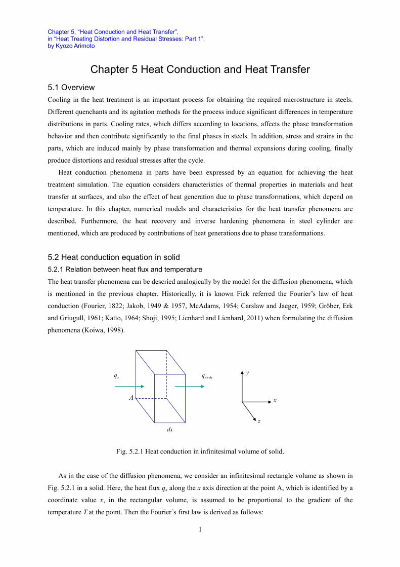
Chapter 5, “Heat Conduction and Heat Transfer”, in “Heat Treating Distortion and Residual Stresses: Part 1”, by Kyozo Arimoto 1 Chapter 5 Heat Conduction and Heat Transfer 5.1 Overview Cooling in the heat treatment is an important process for obtaining the required microstructure in steels. Different quenchants and its agitation methods for the process induce significant differences in temperature distributions in parts. Cooling rates, which differs according to locations, affects the phase transformation behavior and then contribute significantly to the final phases in steels. In addition, stress and strains in the parts, which are induced mainly by phase transformation and thermal expansions during cooling, finally produce distortions and residual stresses after the cycle. Heat conduction phenomena in parts have been expressed by an equation for achieving the heat treatment simulation. The equation considers characteristics of thermal properties in materials and heat transfer at surfaces, and also the effect of heat generation due to phase transformations, which depend on temperature. In this chapter, numerical models and characteristics for the heat transfer phenomena are described. Furthermore, the heat recovery and inverse hardening phenomena in steel cylinder are mentioned, which are produced by contributions of heat generations due to phase transformations. 5.2 Heat conduction equation in solid 5.2.1 Relation between heat flux and temperature The heat transfer phenomena can be descried analogically by the model for the diffusion phenomena, which is mentioned in the previous chapter. Historically, it is known Fick referred the Fourier’s law of heat conduction (Fourier, 1822; Jakob, 1949 & 1957, McAdams, 1954; Carslaw and Jaeger, 1959; Gröber, Erk and Griugull, 1961; Katto, 1964; Shoji, 1995; Lienhard and Lienhard, 2011) when formulating the diffusion phenomena (Koiwa, 1998). x dx q + x q A dx y x z Fig. 5.2.1 Heat conduction in infinitesimal volume of solid. As in the case of the diffusion phenomena, we consider an infinitesimal rectangle volume as shown in Fig. 5.2.1 in a solid. Here, the heat flux q x along the x axis direction at the point A, which is identified by a coordinate value x, in the rectangular volume, is assumed to be proportional to the gradient of the temperature T at the point. Then the Fourier’s first law is derived as follows:
Transcript
Chapter 5, “Heat Conduction and Heat Transfer”, in “Heat Treating Distortion and Residual Stresses: Part 1”, by Kyozo Arimoto
1
Chapter 5 Heat Conduction and Heat Transfer 5.1 Overview Cooling in the heat treatment is an important process for obtaining the required microstructure in steels.
Different quenchants and its agitation methods for the process induce significant differences in temperature
distributions in parts. Cooling rates, which differs according to locations, affects the phase transformation
behavior and then contribute significantly to the final phases in steels. In addition, stress and strains in the
parts, which are induced mainly by phase transformation and thermal expansions during cooling, finally
produce distortions and residual stresses after the cycle.
Heat conduction phenomena in parts have been expressed by an equation for achieving the heat
treatment simulation. The equation considers characteristics of thermal properties in materials and heat
transfer at surfaces, and also the effect of heat generation due to phase transformations, which depend on
temperature. In this chapter, numerical models and characteristics for the heat transfer phenomena are
described. Furthermore, the heat recovery and inverse hardening phenomena in steel cylinder are
mentioned, which are produced by contributions of heat generations due to phase transformations.
5.2 Heat conduction equation in solid 5.2.1 Relation between heat flux and temperature
The heat transfer phenomena can be descried analogically by the model for the diffusion phenomena, which
is mentioned in the previous chapter. Historically, it is known Fick referred the Fourier’s law of heat
and Griugull, 1961; Katto, 1964; Shoji, 1995; Lienhard and Lienhard, 2011) when formulating the diffusion
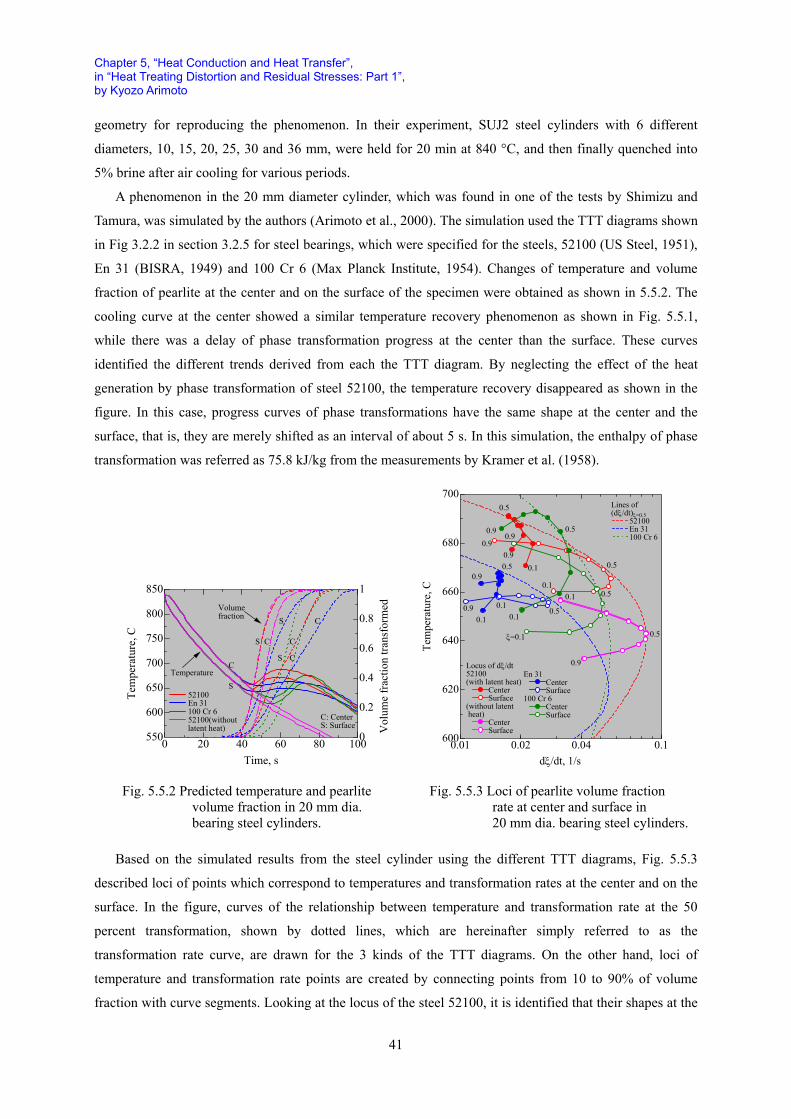
phenomena (Koiwa, 1998).
x dxq + xq
A
dx
y
x
z
Fig. 5.2.1 Heat conduction in infinitesimal volume of solid.
As in the case of the diffusion phenomena, we consider an infinitesimal rectangle volume as shown in
Fig. 5.2.1 in a solid. Here, the heat flux qx along the x axis direction at the point A, which is identified by a
coordinate value x, in the rectangular volume, is assumed to be proportional to the gradient of the
temperature T at the point. Then the Fourier’s first law is derived as follows:
Chapter 5, “Heat Conduction and Heat Transfer”, in “Heat Treating Distortion and Residual Stresses: Part 1”, by Kyozo Arimoto
2
xTq kx
∂= −
∂ (5.2.1)
where, k, T, and qx are heat conductivity, temperature and heat flux, respectively. Since the heat flux qx is
the amount of heat passing through per unit area and time, and then its unit can be expressed as J/(m2s).
When the units of T and ∂T/∂x are specified as °C and °C/m, respectively, the thermal conductivity k is
measured in W/(m °C) based on Eq. (5.2.1).
On the other hand, the temperature change at any point in a solid can be represented by the following
partial differential equations.
T TC kt x x
ρ ∂ ∂ ∂ = ∂ ∂ ∂ (5.2.2)
The above relation is called as the Fourier's second law, and ρ and C are density, kg/m3, and specific heat,
kJ/kg/°C, respectively, which can be derived based on the heat balance in the rectangle shown in Fig. 5.2.1.
The thermal diffusivity, a=k/(ρC), m2/s, can be found in Eq. (5.2.2), which corresponds to the diffusivity in
the diffusion phenomena in Chapter 4.
During heat treatment processes, heat generations occur in steel parts by plastic deformation works and
phase transformations, and also the Joule heating due to electric currents. Now, considering the above heat
generations and heat flows along the y and z axis to Eq. (5.2.2), a general heat conduction equation is
derived as follows:
W J LT T T TC k k k Q Q Qt x x y y z z
ρ ∂ ∂ ∂ ∂ ∂ ∂ ∂ = + + + + + ∂ ∂ ∂ ∂ ∂ ∂ ∂
(5.2.3)
where WQ , JQ and LQ are the heat generation rates due to plastic deformation works, Joule heating and
phase transformations, respectively.
To solve the heat conduction equation for practical problems is needed to specify the initial and
boundary conditions described in the next section. In addition, analyses of the phenomena in complex
shapes are performed based on the finite element method described in Chapter 9.
A significant fraction of the plastic strain energy caused by the work is converted to heat (Elam, 1935). For simplicity, assuming this conversion is completely done, the heat generation rate WQ due to the plastic
deformation works is descried as follows (Mendelson, 1968):
W PQ σ ε= (5.2.4)
where σ and Pε are the effective stress and the effective plastic strain rate, respectively. The unit of
plastic deformation work is W/m3, when the units of stress and strain rate are Pa (= N/m2) and 1/s,
respectively.
The Joule heating is generated, for examples, by eddy currents during induction heating processes. Its rate JQ is derived by specifying the current density i and the electrical resistivity ρ as follows (Kinbara,
1972):
Chapter 5, “Heat Conduction and Heat Transfer”, in “Heat Treating Distortion and Residual Stresses: Part 1”, by Kyozo Arimoto
3
2 JQ iρ= (5.2.5)
where the unit of the Joule heating is W/m3, when using units of the current density and the electrical
resistivity are A/m2 and Ωm, respectively. The theory of high frequency induction heating is described in
Chapter 7. In addition, the heat generation rate LQ due to phase transformations is determined as follows
(Agarwal and Brimacombe, 1981):
LIJ IJQ L ξ=∑ (5.2.6)
where LIJ is the total amount of heat generation due to the phase transformation from phase I to J. In addition, IJξ is the change rate of phase volume fraction due to the phase transformation from phase I to J,
which is called as the transformation rate. The unit of the heat generation is W/m3 when using the units of
total heat generation due to phase transformations and transformation rate are J/m3 and 1/s, respectively. If
the unit of heat generation due to phase transformations is measured in the heat per unit mass, for example,
J/kg, LIJ in Eq. (5.2.6) is obtained by converting of such units by multiplying the density of material to the
above amount.
5.2.2 Initial and boundary conditions
For solving heat conduction phenomena in practical parts, it is necessary to specify initial and boundary
conditions for the heat conduction equation. As for a typical initial condition, a uniform temperature is
specified throughout a solid at the starting of a cycle of heat treatment.
As for boundary conditions, when temperatures on a surface are known as Ts, it is possible to directly
specify the temperature as follows:
( ) 0 SxT T
== (5.2.7)
In the above equation, one-dimensional problem along only the x axis is used as an example for
convenience, and x=0 corresponds to the surface. This is the same to different boundary conditions below.
On the other hand, heat flux qx=0 at the surface may be specified directly as boundary conditions as
follows:
00
xx
Tk qx =
=
∂ − = ∂ (5.2.8)
However, a model of heat transfer boundary can often represent more realistic conditions, which is shown
as follows:
( )0x e sq T Tα= = − (5.2.9)
where α is the heat transfer coefficient, while Te and Ts are the temperatures in an environment and at the
solid surface.
Unit of the heat transfer coefficient is W/(m2 °C), when heat flux qx=0 is J/(m2 s) and temperature T
Chapter 5, “Heat Conduction and Heat Transfer”, in “Heat Treating Distortion and Residual Stresses: Part 1”, by Kyozo Arimoto
4
is °C. In the heat treatment simulation, the heat transfer coefficient for cooling into quenchants depends
commonly on surface temperatures of heat treated parts.
5.3 Thermal properties of steels The heat conduction analysis operated in the heat treatment simulation needs data of specific heat, enthalpy
of transformations, thermal conductivity and density of steels. These thermal properties have been
measured by an inherent method of each individual scientist through the ages; especially a considerable
data has been accumulated for steels.
Here, specific heat, thermal conductivity and enthalpy of transformation in pure iron, carbon steels and
alloy steels are introduced from literatures, and then their adequacy are investigated for applying them to
the current heat treatment simulation. The density is discussed in the next chapter.
5.3.1 Specific heat
First of all, it should be confirmed what the specific heat is. If heat ∆Q is needed when changing the
temperature ∆T in an object with mass M, and the specific heat C is expressed as follows:
1 QCM T
∆=
∆ (5.3.1)
For the unit of the specific heat, kJ/(kg °C) is often used. On the other hand, the specific heat in a mole of
substance is measured in the unit of J/(mol °C).
When a specific heat is derived based on Eq. (5.3.1), the temperature of a solid should be uniform. It is
difficult to achieve exactly under the above condition in measurements; therefore, the obtained data would
contain errors. In addition, the specific heat of solid is measured usually in constant pressure.
A theoretical estimation of the specific heat of metal has been attempted to divide it to vibrational,
electronic and magnetic effects (Nishizawa, 1973). The above effects on specific heat can correlate with
crystal lattice vibrations, electronic excitation of free electron, and atomic spin equilibrium in
ferromagnetic alloy. Even though the theoretical study is effective to understand this kind of phenomenon,
specific heat data for individual substances are eventually confirmed by measurements.
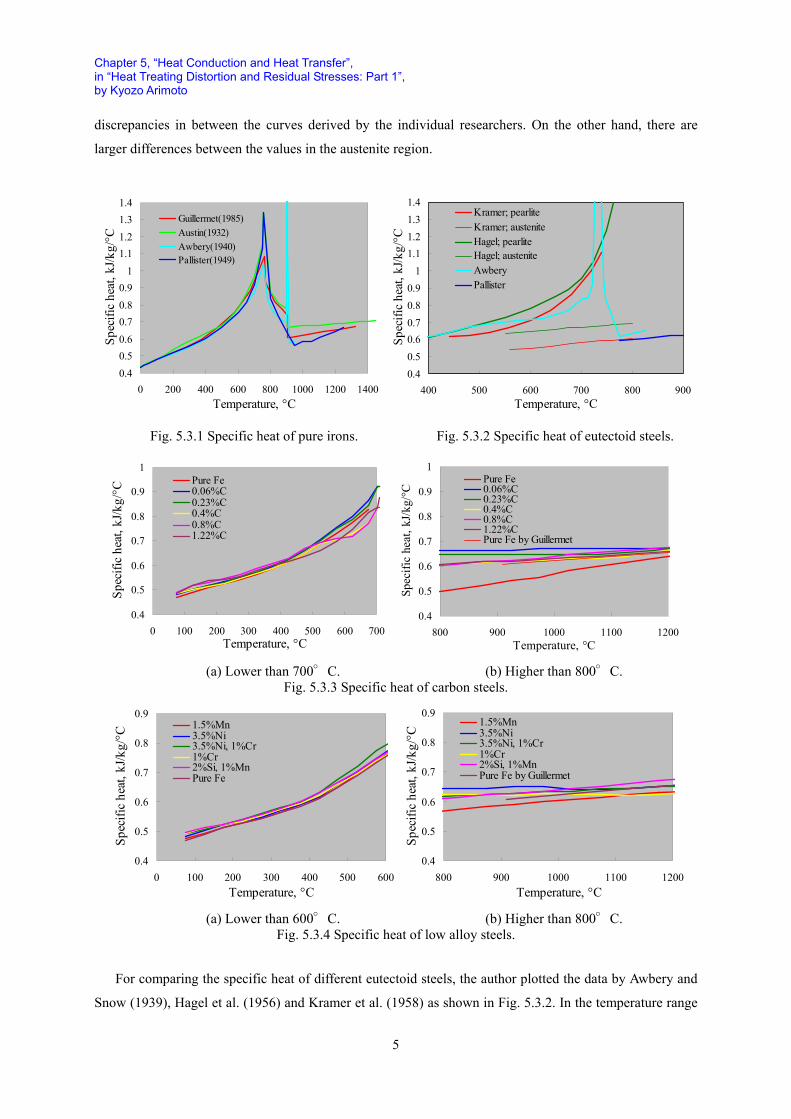
For the specific heat of pure iron, measured data in the 1930s have been assessed by Austin (1932).
Subsequently, Griffiths-Awbery (1940) and Pallister (1949) reported specific heat data measured using the
Sykes (1936) method and the electric current heating method, respectively. In more recent years,
Guillermet and Gustafson (1985) obtained specific heat curves by the thermodynamic assessment based on
past measured data. Figure 5.3.1 was made by the author to compare the above four kinds of specific heat
data in pure iron.
As shown in Fig.5.3.1, a peak appears in each specific heat curve in the range of from 600 to 800 °C,
which is induced by magnetic transformations. As for the peak values, the measurement by Awbery and
Griffiths agrees well with Guillermet and Gustafson’s. However, these values are quite smaller than the
measured data by Pallister and Austin. In the lower range of temperature than the peaks, there are small
Chapter 5, “Heat Conduction and Heat Transfer”, in “Heat Treating Distortion and Residual Stresses: Part 1”, by Kyozo Arimoto
5
discrepancies in between the curves derived by the individual researchers. On the other hand, there are
larger differences between the values in the austenite region.
Fig. 5.3.1 Specific heat of pure irons. Fig. 5.3.2 Specific heat of eutectoid steels.
0.4
0.5
0.6
0.7
0.8
0.9
1
0 100 200 300 400 500 600 700Temperature, °C
Spec
ific
heat
, kJ/k
g/°C
Pure Fe0.06%C0.23%C0.4%C0.8%C1.22%C
0.4
0.5
0.6
0.7
0.8
0.9
1
800 900 1000 1100 1200Temperature, °C
Spec
ific
heat
, kJ/
kg/°
C
Pure Fe0.06%C0.23%C0.4%C0.8%C1.22%CPure Fe by Guillermet
(a) Lower than 700°C. (b) Higher than 800°C.
Fig. 5.3.3 Specific heat of carbon steels.
0.4
0.5
0.6
0.7
0.8
0.9
0 100 200 300 400 500 600Temperature, °C
Spec
ific
heat
, kJ/k
g/°C
1.5%Mn3.5%Ni3.5%Ni, 1%Cr1%Cr2%Si, 1%MnPure Fe
0.4
0.5
0.6
0.7
0.8
0.9
800 900 1000 1100 1200Temperature, °C
Spec
ific
heat
, kJ/k
g/°C
1.5%Mn3.5%Ni3.5%Ni, 1%Cr1%Cr2%Si, 1%MnPure Fe by Guillermet
(a) Lower than 600°C. (b) Higher than 800°C.
Fig. 5.3.4 Specific heat of low alloy steels.
For comparing the specific heat of different eutectoid steels, the author plotted the data by Awbery and
Snow (1939), Hagel et al. (1956) and Kramer et al. (1958) as shown in Fig. 5.3.2. In the temperature range
Chapter 5, “Heat Conduction and Heat Transfer”, in “Heat Treating Distortion and Residual Stresses: Part 1”, by Kyozo Arimoto
6
of pearlite, there are discrepancies in between data measured by Hagel et al. and Kramer et al. using the
Smith (1940) method, and by Awbery and Snow using the Sykes (1936) method. Especially, in the range
from 600 to 700 °C, data by Awbery and Snow shows a lower value than others. Meanwhile, in the
austenite region, a discrepancy in between data by Pallister and Kramer et al. is small. However, there is a
discrepancy in between data by Kramer et al. and Hagel et al., both which used the same Smith method.
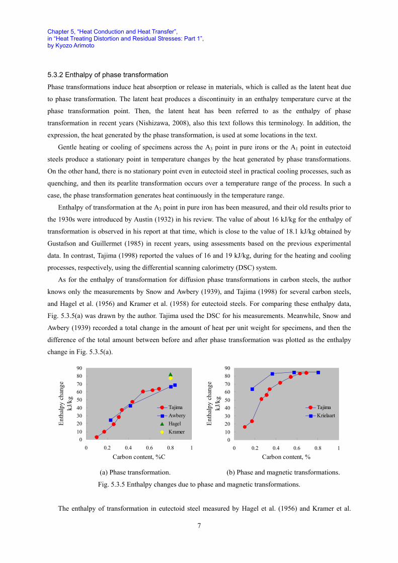
Hagel et al. and Kramer et al. measured only for the eutectoid steels, while Awbery and Snow (1939)
and Pallister (1946) broadened the range to the data for carbon steels and other alloy steels. The author
depicted specific heat curves by selecting the carbon steel data up to 700 °C from the data by Awbery and
Snow as shown in Fig. 5.3.3 (a). It is difficult to find some regularity of the carbon concentration
dependency in the specific heat from this figure. The data for pure iron in this figure was obtained by
Griffiths and Awbery (1940).
Fig. 5.3.3 (b) was created for comparing the specific heat of different carbon steels in the austenite
region. The specific heat curves included here were measured by Pallister(1946), except the data of pure
iron by Gustafson and Guillermet (1985). As already mentioned, the specific heat curves of pure iron by
Guillermet and Gustafson differ from Pallister’s. However, the specific heat curves of carbon steels
becomes almost horizontal and their discrepancies are within the range of 0.05 kJ/(kg °C).
On the other hand, the specific heat for various low-alloy steel up to 600 °C, which was measured by
Awbery and Challoner (1946), were compared by the author as shown in Fig 5.3.4 (a). Carbon
concentration of the steels in the figure is in the range of about 0.2 to 0.5% C. The Difference between the
specific heat curves for the steels is 0.05 kJ/ (kg °C), therefore, carbon may not so affect to the specific heat
when Si, Mn, Cr and Ni are within the range shown in the figure. Curves of the low-alloy steels are all
located above the pure iron, which was drawn for comparison. In addition, the specific heat curves of alloy
steels in the austenite region show substantially a horizontal distribution as depicted in Fig. 5.3.4 (b), which
are within the range of about 0.005 kJ/(kg °C).
To investigate the effect of alloying elements on the specific heat, Pallister (1946) plotted data of the
specific heat in a variety of carbon steels and alloy steels at 1250 °C, specifying the number of atoms
contained in 100 g of steel as the horizontal axis. As a result, he found a tendency that specific heat was
raised with increasing number of atoms. For example, specific heat is higher in the steel which includes
many lighter elements such as carbon; reversely steels including a few heavy elements such as tungsten
make it lower. However, this trend appeared in the austenite region.
The specific heat data measured by Awbery and Snow (1939), Awbery and Challoner (1946) and
Pallister (1946) were published as the data book from British Iron and Steel Research Association (BISRA)
(1953). Now, specific heat of steels with given chemical compositions can be predicted by thermodynamic
software (Saunders and Miodownik, 1998). In addition, the prediction by such software needs the database
of the free energy for each element and the interaction parameters between elements. Specific heat data of
pure iron by Guillermet and Gustafson has been adopted by such a database (Dinsdale, 1991). In addition,
Miettinen (1997) reported on the prediction method of specific heat based on the somewhat simplified
thermodynamic approach.
Chapter 5, “Heat Conduction and Heat Transfer”, in “Heat Treating Distortion and Residual Stresses: Part 1”, by Kyozo Arimoto
7
5.3.2 Enthalpy of phase transformation
Phase transformations induce heat absorption or release in materials, which is called as the latent heat due
to phase transformation. The latent heat produces a discontinuity in an enthalpy temperature curve at the
phase transformation point. Then, the latent heat has been referred to as the enthalpy of phase
transformation in recent years (Nishizawa, 2008), also this text follows this terminology. In addition, the
expression, the heat generated by the phase transformation, is used at some locations in the text.
Gentle heating or cooling of specimens across the A3 point in pure irons or the A1 point in eutectoid
steels produce a stationary point in temperature changes by the heat generated by phase transformations.
On the other hand, there is no stationary point even in eutectoid steel in practical cooling processes, such as
quenching, and then its pearlite transformation occurs over a temperature range of the process. In such a
case, the phase transformation generates heat continuously in the temperature range.
Enthalpy of transformation at the A3 point in pure iron has been measured, and their old results prior to
the 1930s were introduced by Austin (1932) in his review. The value of about 16 kJ/kg for the enthalpy of
transformation is observed in his report at that time, which is close to the value of 18.1 kJ/kg obtained by
Gustafson and Guillermet (1985) in recent years, using assessments based on the previous experimental
data. In contrast, Tajima (1998) reported the values of 16 and 19 kJ/kg, during for the heating and cooling
processes, respectively, using the differential scanning calorimetry (DSC) system.
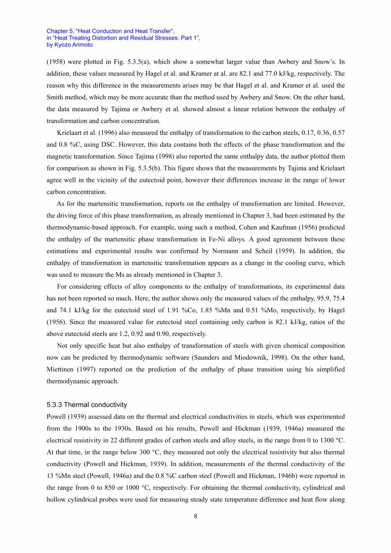
As for the enthalpy of transformation for diffusion phase transformations in carbon steels, the author
knows only the measurements by Snow and Awbery (1939), and Tajima (1998) for several carbon steels,
and Hagel et al. (1956) and Kramer et al. (1958) for eutectoid steels. For comparing these enthalpy data,
Fig. 5.3.5(a) was drawn by the author. Tajima used the DSC for his measurements. Meanwhile, Snow and
Awbery (1939) recorded a total change in the amount of heat per unit weight for specimens, and then the
difference of the total amount between before and after phase transformation was plotted as the enthalpy
change in Fig. 5.3.5(a).
0102030405060708090
0 0.2 0.4 0.6 0.8 1
Carbon content, %C
Enth
alpy
cha
nge
kJ/k
g
TajimaAwberyHagelKramer
0102030405060708090
0 0.2 0.4 0.6 0.8 1
Carbon content, %
Enth
alpy
cha
nge
kJ/k
g
TajimaKrielaart
(a) Phase transformation. (b) Phase and magnetic transformations.
Fig. 5.3.5 Enthalpy changes due to phase and magnetic transformations.
The enthalpy of transformation in eutectoid steel measured by Hagel et al. (1956) and Kramer et al.
Chapter 5, “Heat Conduction and Heat Transfer”, in “Heat Treating Distortion and Residual Stresses: Part 1”, by Kyozo Arimoto
8
(1958) were plotted in Fig. 5.3.5(a), which show a somewhat larger value than Awbery and Snow’s. In
addition, these values measured by Hagel et al. and Kramer at al. are 82.1 and 77.0 kJ/kg, respectively. The
reason why this difference in the measurements arises may be that Hagel et al. and Kramer et al. used the
Smith method, which may be more accurate than the method used by Awbery and Snow. On the other hand,
the data measured by Tajima or Awbery et al. showed almost a linear relation between the enthalpy of
transformation and carbon concentration.
Krielaart et al. (1996) also measured the enthalpy of transformation to the carbon steels, 0.17, 0.36, 0.57
and 0.8 %C, using DSC. However, this data contains both the effects of the phase transformation and the
magnetic transformation. Since Tajima (1998) also reported the same enthalpy data, the author plotted them
for comparison as shown in Fig. 5.3.5(b). This figure shows that the measurements by Tajima and Krielaart
agree well in the vicinity of the eutectoid point, however their differences increase in the range of lower
carbon concentration.
As for the martensitic transformation, reports on the enthalpy of transformation are limited. However,
the driving force of this phase transformation, as already mentioned in Chapter 3, had been estimated by the
thermodynamic-based approach. For example, using such a method, Cohen and Kaufman (1956) predicted
the enthalpy of the martensitic phase transformation in Fe-Ni alloys. A good agreement between these
estimations and experimental results was confirmed by Normann and Scheil (1959). In addition, the
enthalpy of transformation in martensitic transformation appears as a change in the cooling curve, which
was used to measure the Ms as already mentioned in Chapter 3.
For considering effects of alloy components to the enthalpy of transformations, its experimental data
has not been reported so much. Here, the author shows only the measured values of the enthalpy, 95.9, 75.4
and 74.1 kJ/kg for the eutectoid steel of 1.91 %Co, 1.85 %Mn and 0.51 %Mo, respectively, by Hagel
(1956). Since the measured value for eutectoid steel containing only carbon is 82.1 kJ/kg, ratios of the
above eutectoid steels are 1.2, 0.92 and 0.90, respectively.
Not only specific heat but also enthalpy of transformation of steels with given chemical composition
now can be predicted by thermodynamic software (Saunders and Miodownik, 1998). On the other hand,
Miettinen (1997) reported on the prediction of the enthalpy of phase transition using his simplified
thermodynamic approach.
5.3.3 Thermal conductivity
Powell (1939) assessed data on the thermal and electrical conductivities in steels, which was experimented
from the 1900s to the 1930s. Based on his results, Powell and Hickman (1939, 1946a) measured the
electrical resistivity in 22 different grades of carbon steels and alloy steels, in the range from 0 to 1300 °C.
At that time, in the range below 300 °C, they measured not only the electrical resistivity but also thermal
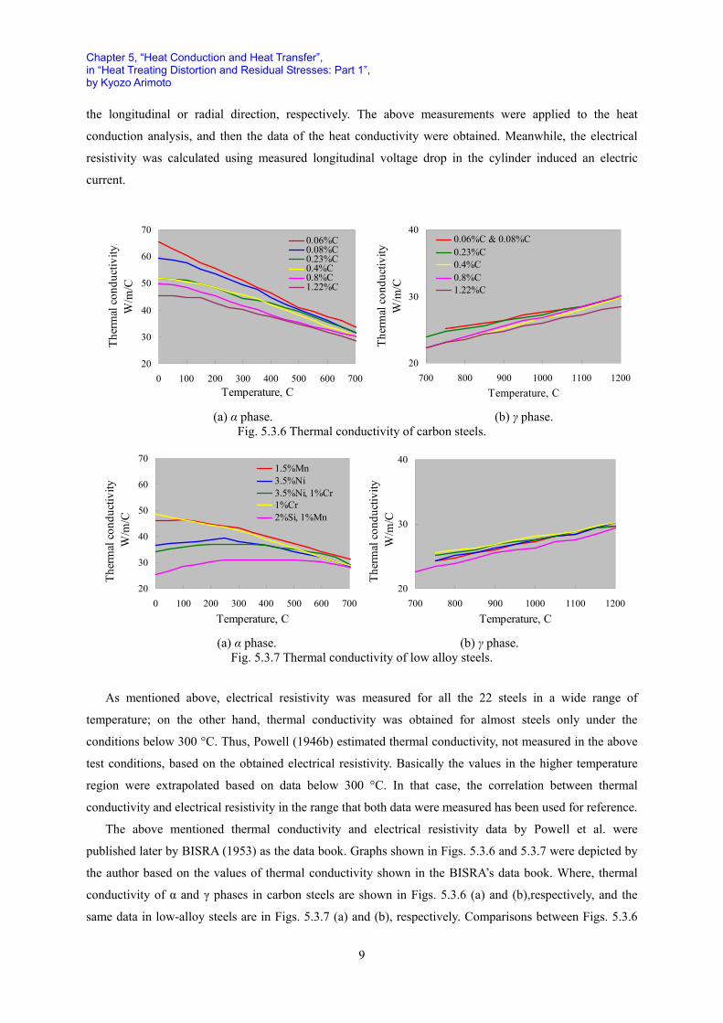
conductivity (Powell and Hickman, 1939). In addition, measurements of the thermal conductivity of the
13 %Mn steel (Powell, 1946a) and the 0.8 %C carbon steel (Powell and Hickman, 1946b) were reported in
the range from 0 to 850 or 1000 °C, respectively. For obtaining the thermal conductivity, cylindrical and
hollow cylindrical probes were used for measuring steady state temperature difference and heat flow along
Chapter 5, “Heat Conduction and Heat Transfer”, in “Heat Treating Distortion and Residual Stresses: Part 1”, by Kyozo Arimoto
9
the longitudinal or radial direction, respectively. The above measurements were applied to the heat
conduction analysis, and then the data of the heat conductivity were obtained. Meanwhile, the electrical
resistivity was calculated using measured longitudinal voltage drop in the cylinder induced an electric
current.
20
30
40
50
60
70
0 100 200 300 400 500 600 700Temperature, C
Ther
mal
con
duct
ivity
,W
/m/C
0.06%C0.08%C0.23%C0.4%C0.8%C1.22%C
20
30
40
700 800 900 1000 1100 1200Temperature, C
Ther
mal
con
duct
ivity
W/m
/C
0.06%C & 0.08%C0.23%C0.4%C0.8%C1.22%C
(a) α phase. (b) γ phase.
Fig. 5.3.6 Thermal conductivity of carbon steels.
20
30
40
50
60
70
0 100 200 300 400 500 600 700Temperature, C
Ther
mal
con
duct
ivity
W/m
/C
1.5%Mn3.5%Ni3.5%Ni, 1%Cr1%Cr2%Si, 1%Mn
20
30
40
700 800 900 1000 1100 1200Temperature, C
Ther
mal
con
duct
ivity
W/m
/C
(a) α phase. (b) γ phase.
Fig. 5.3.7 Thermal conductivity of low alloy steels.
As mentioned above, electrical resistivity was measured for all the 22 steels in a wide range of
temperature; on the other hand, thermal conductivity was obtained for almost steels only under the
conditions below 300 °C. Thus, Powell (1946b) estimated thermal conductivity, not measured in the above
test conditions, based on the obtained electrical resistivity. Basically the values in the higher temperature
region were extrapolated based on data below 300 °C. In that case, the correlation between thermal
conductivity and electrical resistivity in the range that both data were measured has been used for reference.
The above mentioned thermal conductivity and electrical resistivity data by Powell et al. were
published later by BISRA (1953) as the data book. Graphs shown in Figs. 5.3.6 and 5.3.7 were depicted by
the author based on the values of thermal conductivity shown in the BISRA’s data book. Where, thermal
conductivity of α and γ phases in carbon steels are shown in Figs. 5.3.6 (a) and (b),respectively, and the
same data in low-alloy steels are in Figs. 5.3.7 (a) and (b), respectively. Comparisons between Figs. 5.3.6
Chapter 5, “Heat Conduction and Heat Transfer”, in “Heat Treating Distortion and Residual Stresses: Part 1”, by Kyozo Arimoto
10
(a) and 5.3.7 (a) show that alloy components decrease thermal conductivity. However, Powell (1946b)
could not perform a quantitative assessment of the effect. Electrical resistivity data contained in the
BISRA’s data book are discussed in Section 7.3.
A measurement of thermal conductivity in steels after the works by Powell et al., which was noticed by
the author, is included in a work by Kobayashi et al. (1987). Where, Fe-C alloys with different carbon
concentrations were used to measure the thermal diffusivity by a transient heating technique using a square
wave pulse. Alloys to measure were produced by dissolving electrolytic iron and carbon in a vacuum
induction melting furnace, and then eight stages of carbon concentrations were adjusted in the range of 0 to
1.4 %C approximately. The measured thermal diffusivity was expressed as an empirical formula which may
estimate a value in from room temperature to 400 °C, and in carbon concentrations from 0 to 1.4 %C.
Influences of the microstructure were investigated by comparisons between measured values in the case of
spherical or plate-like cementites, however significant differences were not been observed.
Kobayashi et al. obtained thermal conductivity based on measurements of specific heat and thermal
diffusivity. The results showed a trend similar to that of BISRA in Fig. 5.3.6, and are somewhat larger in
perspective. The indicated value of the density used in obtaining the thermal conductivity from thermal
diffusivity is likely to be measured at room temperature. In addition, electrical resistivity measured by
Kobayashi et al. is introduced in Section 7.3.
In late years, Miettinen (1997) derived an empirical formula on thermal conductivity, considering the
dependence of chemical composition, including C, Si, Mn, Cr, Mo and Ni, based on past experimental data.
In addition, this experimental expression is intended to obtain the thermal conductivity at 25, 200 and
400 °C. Furthermore, dependence of temperature as well as alloy components was represented by a
polynomial in austenite region.
5.4 Heat transfer during heat treating Generally, waters, oils, polymer solutions and gases have been used for quenchants (Totten et al., 1993).
Studies on the heat transfer in mainly liquid quenchants were reviews in this text. It is known that a cooling
process in the liquid quenchants is usually divided into three stages, vapor film, boiling and convection. In
addition, quenchants are often used with an agitation which affects their heat transfer in cooling.
Phenomena of heat transfer during boiling of liquids have been studied for the heat exchange in
equipments such as boilers, heat exchangers and unclear reactors, and then many significant results
reported as a part of textbook (Jakob, 1949 & 1957, McAdams, 1954; Gröber, Erk and Griugull, 1961;
Katto, 1964; Shoji, 1995) or for example a specific publication (Japan Society of Mechanical Engineers,
1965). In experiments on boiling heat transfer phenomena, a probe has usually a heating source in its inside,
which controls temperature. On the other hand, a probe for the phenomena during heat treatment does not
control their temperature in any way.
It may be difficult that complex behaviors in quenchants during cooling in the quenching, such as vapor
film generations and boiling, are simulated directly under modern technologies. Therefore, in the current
heat treatment simulation, the model of heat transfer boundary described as Eq. (5.2.9) has been applied to
Chapter 5, “Heat Conduction and Heat Transfer”, in “Heat Treating Distortion and Residual Stresses: Part 1”, by Kyozo Arimoto
11
surfaces of heat treated parts.
The following sections outline results of studies on cooling during heat treatment. History of researches
on measurements of the cooling and cooling rate curves, and the H value, the severity of quench, derived
from an analytical study of heat transfer are described. Meanwhile, the author outlines a platinum wire
method used for the study of heat transfer through the ages, and its expansion to measure in the vapor film
stage. In addition, the methods of lumped heat capacity, inverse analysis, CFD (Computational Fluid
Dynamics), and so on, for predicting heat transfer coefficients are summarized. Finally, an outlook on
deriving heat transfer coefficients for heat treatment simulation is discussed.
5.4.1 Cooling curves and cooling rate curves
Studies on cooling phenomena during quenching were started by measuring temperature changes in a probe
with a simple geometry, which is immersed into a variety of quenchants. A chart recorded a temperature
change is called as the cooling curve. It is difficult to trace back to a beginning of the research on this
curve.
Here, from studies by Benedicks(1908), recognized as a pioneer in this field by many researchers in
their literatures, to recent researches are introduced in chronological order. Furthermore, also the cooling
rate curves are discussed, which were obtained from the cooling curves in early researches in this field.
(1) From 1900 to 1929
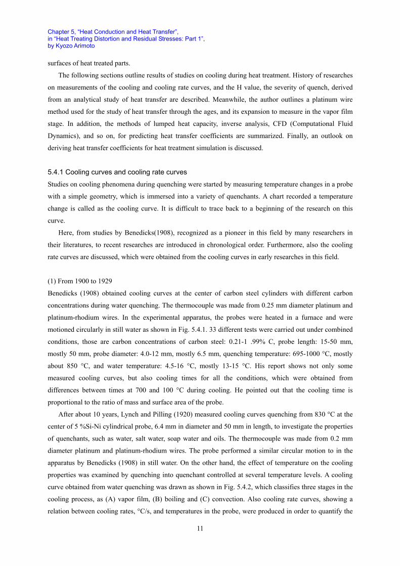
Benedicks (1908) obtained cooling curves at the center of carbon steel cylinders with different carbon
concentrations during water quenching. The thermocouple was made from 0.25 mm diameter platinum and
platinum-rhodium wires. In the experimental apparatus, the probes were heated in a furnace and were
motioned circularly in still water as shown in Fig. 5.4.1. 33 different tests were carried out under combined
conditions, those are carbon concentrations of carbon steel: 0.21-1 .99% C, probe length: 15-50 mm,
mostly 50 mm, probe diameter: 4.0-12 mm, mostly 6.5 mm, quenching temperature: 695-1000 °C, mostly
about 850 °C, and water temperature: 4.5-16 °C, mostly 13-15 °C. His report shows not only some
measured cooling curves, but also cooling times for all the conditions, which were obtained from
differences between times at 700 and 100 °C during cooling. He pointed out that the cooling time is
proportional to the ratio of mass and surface area of the probe.
After about 10 years, Lynch and Pilling (1920) measured cooling curves quenching from 830 °C at the
center of 5 %Si-Ni cylindrical probe, 6.4 mm in diameter and 50 mm in length, to investigate the properties
of quenchants, such as water, salt water, soap water and oils. The thermocouple was made from 0.2 mm
diameter platinum and platinum-rhodium wires. The probe performed a similar circular motion to in the
apparatus by Benedicks (1908) in still water. On the other hand, the effect of temperature on the cooling
properties was examined by quenching into quenchant controlled at several temperature levels. A cooling
curve obtained from water quenching was drawn as shown in Fig. 5.4.2, which classifies three stages in the
cooling process, as (A) vapor film, (B) boiling and (C) convection. Also cooling rate curves, showing a
relation between cooling rates, °C/s, and temperatures in the probe, were produced in order to quantify the
Chapter 5, “Heat Conduction and Heat Transfer”, in “Heat Treating Distortion and Residual Stresses: Part 1”, by Kyozo Arimoto
12
cooling characteristics. In addition, the cooling rate was called as quenching power by Lynch and Pilling.
Furnace Specimen
Tank
0100200300400500600700800900
0 1 2 3 4 5 6 7 8 9 10 11 12 13 14 15
Time, s
Tem
pera
ture
, °C
A B C
Fig. 5.4.1 Benedicks’s apparatus. Fig. 5.4.2 Cooling curve measured in water at 58 °C from 830 °C.
Scott (1924) measured cooling curves at the center of the Fe-32 %Ni alloy cylindrical probe, 1 in (25.4
mm) in diameter, during their quenching into water, several concentrations of glycerol solutions, oil-water
emulsions and oils. Two quenching temperatures, 100 and 800 °C, were tried for these tests. He showed the
effect of different kinds of quenchants and different concentrations of glycerol water on the cooling
properties based on the shapes of obtained cooling curves. In his subsequent report (Scott, 1934a), cooling
curves were measured during water quenching from 100 or 750 °C at the center and the position which is
0.84 in (21.3 mm) from the center, in the Fe-32 %Ni alloys cylindrical probe, 2 in (50.8 mm) in diameter.
Then, he obtained theoretical results of heat transfer phenomena in terms of these measurement conditions,
which were compared with experimental results.
(2) From 1930 to 1939
Cooling curves were reported by French (1930a, 1930b), which were measured in steel cylinder, sphere and
plate probes quenched into a variety of quenchants. This result is a compilation of studies over the past 6
years in the U. S. Bureau of Standards. In cylindrical and spherical probes, their diameters were varied
step-by-step in the range 1/2-11 in (12.7-280 mm). Cooling curves were measured by the thermocouple,
which was made from platinum and platinum-rhodium wires, on the surface or at the center of the probes.
Probes were made of not only carbon steels but also Cr steels. The quenchants were selected from waters,
sodium hydroxides, brines, oils, air, etc., and effects of the agitation on their properties were examined. The
agitation was performed by rotating the cylindrical cooling tank at a constant speed, and its degree was
adjusted by setting the distance between the probe and the center of cooling tank.
On the other hand, French quenched probes, which were a different dimension of cylinders, spheres and
plates, from 875 °C into many kinds of quenchants. The cooling rate V at 720 ° C were derived by cooling
curves at the center of the probe, and then empirical formula:
Chapter 5, “Heat Conduction and Heat Transfer”, in “Heat Treating Distortion and Residual Stresses: Part 1”, by Kyozo Arimoto
13
nVD c= (5.4.1) was obtained commonly for various probe shapes. Where, D is diameter of cylinders or spheres, or
thickness of plates, and also n and c are experimental coefficients. It was pointed out that n depends on the
type of quenchants, not on the shape of the probes, while c relates to both types of quenchants and the
shapes of probes. French examined effects of surface roughness and oxidation, gases contained in
quenchants, agitation, cooling spray, etc.
On the other hand, Obinata (1930) measured cooling curves at the center of a α brass cylindrical probe,
10 mm in diameter and 30 mm in length. The thermocouple was made from 0.5 mm diameter platinum and
platinum-rhodium wires. Probes were quenched from 752 °C into water (at 0 to 100 °C), oils (Shirashime
and transformer oils), liquid air and toluol. Not only cooling curves but also cooling rate curves were
created according to the work by Lynch and Pilling (1920).
Using stepped cylindrical probe, 45 or 75 mm in diameter, 150 mm in length each, made of austenitic
stainless steel (14.8 Ni-7.8 Cr), Obata (1931) measured cooling curves at the center of the 75 mm diameter
cylinder during quenching into rape seed oils. The thermocouple was made from platinum and
platinum-rhodium wires. The oils were classified as old, new and their mixtures. Their properties, specific
gravity, free organic acidity, flash point, viscosity, etc. were measured. Oil temperatures were controlled at
25 °C and the other values, which were set at 10 °C intervals in the range from 40 to 100 °C. Comparing
the time required for cooling from 800 to 200 °C, it was reported that the fastest was new oil, and mixed
and old oils were second and third, respectively. Also, it was pointed out that the cooling time was
essentially increased with rising oil temperature in any oils. .
Using Cr-Ni steel ball probes, 4 mm in diameter, Wever (1932) was performed quench experiments for
different cooling conditions (Houdremont, 1956). Experimental results were plotted as relations between
cooling rates and temperatures at several stages during cooling.
Sato (1933) quenched probes coated on the surface from 800 °C for examining the effect of facing
based on obtained cooling curves. A probe was cylinder, 6 mm in diameter and 70 mm in length, made of
Fe-20 %Cr-20 %Ni-alloy, its surface coated with soup which was made as a mixture of clay, graphite
powder, abrasive grain, baked borax and water. Waters with different temperatures, glycerols and several
oils were used for quenchants. Except for some oil, it made clear that the cooling time of quenching was
reduced by the presence of the coating. Examining movies on the cooling phenomena, it was confirmed
that the absence of the coating produced a vapor film covering the probe just after cooling, while the
existence made generating active fine steam foams on the probe surface from the beginning of cooling. In
addition, the Sato’s apparatus measured temperature changes by converting it from the thermal contraction
of the probe. The similar approach was succeeded by the apparatus by Ishihara and Ichihara (1942) for
measuring length changes during quenching. Further studies (Narazaki et al., 1988; Inoue and Uehara,
1995) on the effect of the coating are seen in recent years.
Using the apparatus devised by Sato (1933), except for 5 mm in probe’s diameter, Hara (1935)
measured cooling curves during quenching from 830 °C into waters, rape seed oils, soybean oils, new and
old fish oils, mixture of old fish oils and vegetable oils. All quenchants were investigated at temperatures
Chapter 5, “Heat Conduction and Heat Transfer”, in “Heat Treating Distortion and Residual Stresses: Part 1”, by Kyozo Arimoto
14
set 20 °C intervals in the range from 20 to 100 °C, and then their cooling curves and cooling rate curves
were created. Moreover, behaviors of not only still but also agitated cooling were reported, however an
agitation method was not described. Comparisons between characteristics of the quenchants based on
average cooling velocities from 800 to 400 °C showed that the values in the agitation is larger than still. In
addition, relations between temperature of quenchants and viscosity, cooling rate and viscosity, viscosity
and cooling rate when adding water to the quenchants, quenching temperature and cooling rate, and also
oxidation of quenchants and viscosity were examined.
Lange and Speith (1935) quenched copper spheres, 10-20 mm in diameter, and photographed using the
schlieren method for examining phenomena occurred in quenchants. Their interests were such as cooling
by turbulent flow in the quenchants, a role of the turbulent or laminar boundary layer, heat dissipation
through a closed vapor blanket and heat exchange on collapse of the vapor blanket. Based on the pictures to
characterize these phenomena, their considerations were described. For the heat dissipation through the
vapor blanket, the existence of a laminar flow of the quenchant around the vapor blanket was pointed out.
In addition, a supporting device was provided at the bottom of the probe to observe clearly various
phenomena in quenchants. Meanwhile, silver sphere probe were quenched waters, brines, lithium chloride
solutions, Pektinit (mainly pectin ingredient) solutions, rape seed oils, sodium palmitate solutions and so on,
and then measured cooling curves at the center were reported. The diameter of the silver sphere used in this
study was 20 mm, which differs from 7 mm in the probe by Engel (1931). The reason for this change in
diameter was instability in smaller probes at the immersion stage. The thermocouple was made from
platinum and platinum-rhodium wires. Confirming further the characteristics of the Pektinit solution
practically, carbon steel cylinders, 24 mm in diameter and 80mm in length, were quenched in the solutions
of different concentrations, and measured surface hardness data were compared.
Russell (1939) adopted a silver sphere to investigate cooling characteristics of quenching oils, which is
similar to the probe used by Lange and Speith (1935). Cooling curves were measured using a thermocouple
at the center of the sphere, 1 in (25.4 mm) in diameter, during quenching from about 850 °C. The
thermocouple was made from platinum and platinum-rhodium wires, 0.006 in (0.15 mm) in diameter.
Probes were made of not only silver, but also austenitic steel (20% Ni-25% Cr), with the same dimensions
for comparisons. Eight kinds of quenching oils were tested, which had different cooling properties.
Property values of the oil, i.e., saponification value, acid value, iodine value, flash point, density, viscosity,
volatility, specific heat, thermal conductivity and so on, were reported by Jones (1939) separately.
Measured cooling curves showed differences between materials of the probe. In the case of silver, a
bending point of the cooling curves were appeared clearly by Russell when moving from vapor blanket to
boiling stages, which was called as the characteristic point. However the austenitic steel did not show the
point explicitly. The temperature at the characteristic point was called as the characteristic temperature in
subsequent studies. Russell examined further cooling curves obtained at the different thermocouple
positions, i.e. on the bottom or the side surfaces in the silver sphere probe. It was found that the cooling rate
was larger on the bottom in the early stage of cooling, while the time to reach to the characteristic point was
shorter at the side.
Chapter 5, “Heat Conduction and Heat Transfer”, in “Heat Treating Distortion and Residual Stresses: Part 1”, by Kyozo Arimoto
15
Using a cylindrical steel probe, Stanfield (1939) examined cooling characteristics of some quenching
oils, which were the same as used in the studies by Russell (1939), and water and air. Probes were made of
four kinds of steels, i.e., low carbon steel, 0.87 %C steel, 3 %Ni-Cr steel and austenitic Cr-Ni steel.
Cylindrical probes, 3 in (76 mm) in diameter and 6 in (152 mm) in length, installed thermocouples at two
places, 0.3 in (7.6 mm) from the center and the surface. The thermocouple was made from platinum and
platinum-rhodium wires, 0.35 mm in diameter. Quenching temperatures included often in the range from
820 to 830 °C were specified, and then their cooling curves were plotted using data obtained at two
thermocouples in the probe. Curves showed differences between oils and also with or without surface
scales, however could not be used to specify the characteristic points.
(3) From 1940 to 1949
Using the 20 mm diameter silver spheres devised by Lange and Speith (1935), Rose (1940) measured
temperature changes by a thermocouple at the center of the probe. The thermocouple was changed from a
0.3 mm platinum/platinum-rhodium to 0.5mm iron/constantine to prevent property changes after repeated
heating. Spheres were supported by a thin-walled neck, 30 mm in length, with a small mass. After heating
the silver sphere at 800 °C, was immersed in quenchants to a depth of about half of the supporting neck,
and then uniformly moved at about 25 cm/s. All experimental results were reported in the form of the
cooling rate curve rather than the cooling curve. In addition, as described later, heat transfer coefficients
were calculated by the lumped heat capacity method. Reported cooling rate curves were obtained from, for
example, airs (still and compressed), waters (temperature dependency), sodium hydroxide solutions,
calcium hydroxide solutions, mineral oils (temperature and property dependencies), rapeseed oils, fish oils,
mixed oils emulsions (oil volume and temperature dependencies), pectin solutions and water glass.
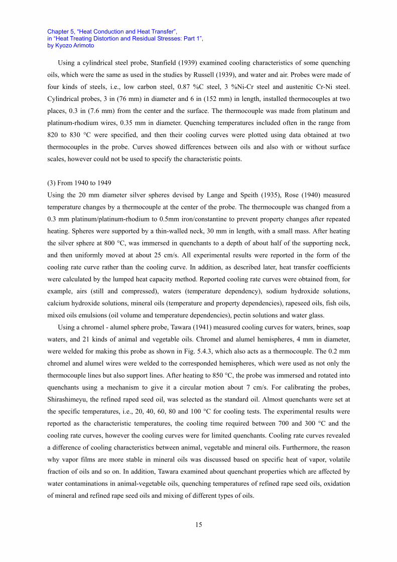
Using a chromel - alumel sphere probe, Tawara (1941) measured cooling curves for waters, brines, soap
waters, and 21 kinds of animal and vegetable oils. Chromel and alumel hemispheres, 4 mm in diameter,
were welded for making this probe as shown in Fig. 5.4.3, which also acts as a thermocouple. The 0.2 mm
chromel and alumel wires were welded to the corresponded hemispheres, which were used as not only the
thermocouple lines but also support lines. After heating to 850 °C, the probe was immersed and rotated into
quenchants using a mechanism to give it a circular motion about 7 cm/s. For calibrating the probes,
Shirashimeyu, the refined raped seed oil, was selected as the standard oil. Almost quenchants were set at
the specific temperatures, i.e., 20, 40, 60, 80 and 100 °C for cooling tests. The experimental results were
reported as the characteristic temperatures, the cooling time required between 700 and 300 °C and the
cooling rate curves, however the cooling curves were for limited quenchants. Cooling rate curves revealed
a difference of cooling characteristics between animal, vegetable and mineral oils. Furthermore, the reason
why vapor films are more stable in mineral oils was discussed based on specific heat of vapor, volatile
fraction of oils and so on. In addition, Tawara examined about quenchant properties which are affected by
water contaminations in animal-vegetable oils, quenching temperatures of refined rape seed oils, oxidation
of mineral and refined rape seed oils and mixing of different types of oils.
Chapter 5, “Heat Conduction and Heat Transfer”, in “Heat Treating Distortion and Residual Stresses: Part 1”, by Kyozo Arimoto
16
Welding
Chromel
Chromel wire (0.2 mm, Dia)
Welding
Alumel
Alumel wire (0.2 mm, Dia)
Pump
FurnaceSpecimen
Tank
Fig. 5.4.3 Chromel - alumel 4mm dia. sphere probe. Fig. 5.4.4 Apparatus by Schallbroch et al.
The test equipment reported by Rose (1940) was improved by Schallbroch et al. (1942) based on an
advice from the Kaiser Wilhelm Institute. Fig. 5.4.4 show the schematic diagram of their apparatus, which
was drawn by the author based on their original. Probe was the 20 mm diameter silver sphere installed a
thermocouple at the center. After heating to 800 °C in an electric furnace, it was immersed in quenchants
until a depth which was not mentioned. Quenchants were circulated normally in a tank by a gear pump at a
flow rate which was not specified. As for using salt bath, a different kind of agitation method, which was
not informed in detail, was used. They reported cooling curves for 4 types of mineral oils, a spindle oil and
rapeseed oil at 80 °C. For a type of mineral oil and the rapeseed oil, effects of temperature on cooling
characteristics were clarified based on the difference in their cooling rate curves. For tap waters, cooling
and cooling rate curves were reported in several temperature levels in the range from 20 °C to the boiling
temperature, which showed obviously the effect of temperature on cooling characteristics. In addition, the
influence of a presence of water and stirring in the salt bath, temperature in calcium chloride solutions on
the cooling curves were reported.
Using cylindrical silver probe, Jones and Pumphrey (1947) obtained cooling curves of waters and oils.
The probe was 3/4 in (19 mm) in diameter and 3 in (76 mm) in length, and had a conical tip of 90 degrees.
A silver - platinum thermocouple was installed at the center of the probe. A cooling tank was installed a jet
orifice to cause around 1 ft/s (30 cm/s) flow on the surface of the probe using a circulating pump. Cooling
curves were obtained from five oils and waters at 20 and 80 °C in agitation, and also for water at 80 °C
without agitation. On the other hand, quenching tests were added using austenitic stainless steel probes to
compare between cooling rate curves obtained from silver and steel probes.
Rose’s Experimental technique (Rose, 1940) using the silver sphere was applied by Peter (1949) to
extensive conditions in a wide range of quenchants (Houdremont, 1956). For example, as for waters,
cooling rate curves were measured for distilled waters, tap waters in Clausthal and Dusseldorf, well waters,
Chapter 5, “Heat Conduction and Heat Transfer”, in “Heat Treating Distortion and Residual Stresses: Part 1”, by Kyozo Arimoto
17
different distilled waters including nitrogen, air, oxygen and carbon dioxide, at the different temperature
levels incremented with 20 °C in a range of from 20 °C to boiling temperature. In addition, cooling
properties were examined for eight different quenching oils, various solutions, metal bathes, salt bathes and
mercury. Meanwhile, Peter (1950) reported separately about effects of surface characteristics on cooling
properties. In this case, using mild steel spheres, 19 and 40 mm in diameter, for example, it was revealed
how cooling rate curves were influenced due to surface oxidations and salt-coated layers.
(4) From 1950 to 1959
Using a silver cylinder, Tagaya and Tamura (1951a) measured cooling curves to examine quenchant
properties. The cylinder, 10 mm in diameter and 30 mm in length, was installed thermocouples, 0.5 mm
chromel-alumel wires, at the center, and a point on the side, which locates up 5 mm in height from the
bottom of the probe. The thermocouples were replaced with the silver-chromel because of anticorrosion,
especially on the surface (Tagaya and Tamura, 1952c). They remarked that the selection of silver was
determined based on the literatures by Lange and Speith (1935), Rose (1940), Peter (1949) and Russell
(1939). Accuracy and repeatability in measurements were cited as an advantage of using silver, while its
higher thermal conductivity than steels was identified as a drawback. They described that the results
obtained from the silver probe could be applied to the problems of quenching steels, under some
considerations. In addition, it was pointed out that the Sato’s cooling apparatus (Sato, 1933) had a problem
of accuracy.
0
100
200
300
400
500
600
700
800
0 0.5 1 1.5 2
Time, s
Tem
pera
ture
, °C
SurfaceCenter
I
II
III
VI
Fig. 5.4.5 Cooling curves measured at surface and center of cylindrical
probe in distilled water at 20 °C from 800 °C.
Tagaya and Tamura (1951b) revealed other stage at the very beginning of the cooling than the stages
classified by Lynch and Pilling (1920) in the cooling curve of water using the silver probe. This was
classified as stage I as shown in Fig. 5.4.5, which was followed by vapor film (II), boiling (III), and
convection (IV) stages. Stage I was described as the process which was for reaching water around the probe
to the boiling point, and can be identified only in cooling curves measured on the surface of the probe.
Meanwhile, the cooling curves on the surface were reported as test results, since the curves at the center
had time delays. In addition, it was described that the stage I was not significant enough to affect the
Chapter 5, “Heat Conduction and Heat Transfer”, in “Heat Treating Distortion and Residual Stresses: Part 1”, by Kyozo Arimoto
18
cooling power (Tagaya and Tamura, 1951c). Cooling curves measured on the bottom surface of silver balls,
as already mentioned by Russell (1939), showed the portion of quick cooling corresponding to the stage I.
For each stage of the cooling, Tagaya and Tamura (1951c) discussed how cooling properties of
quenchants contribute their properties. For example, it was described that the existence of vapor film stage
and its durations relate to molecular structures of quenchants, in particular their shape and polarity, vapor
pressure and vaporization heat. On the other hand, they clarified that the temperature at the end of vapor
film stage, the characteristic temperature in the distilled waters at 20 °C did not depend on their quenching
temperature from the experimental results. As for LiCl, NaCl and KCl solutions, it was found that the
characteristic temperature was raised by increasing their concentration, which was explained by the polarity
of each solution. In addition, their cooling curves of distilled water at 20 °C showed that temperature
decreased in the stage I became larger with increasing the quenching temperature.
Tagaya and Tamura measured cooling curves for a variety of quenchants, i.e., water and liquids
composed mainly water (Tagaya and Tamura, 1952a), animal and vegetable oils (Tagaya and Tamura,
1952b), concentrated salt solutions (Tagaya and Tamura, 1952c) and mineral oils (Tagaya and Tamura,
1953) in a wide range of their conditions. In addition, they summarized tabular forms in contrast to an
average cooling rate in temperature ranges for pearlite (700-500 °C) and martensite (300-200 °C).
Using cylindrical silver probes, 4 different diameters, 10, 15, 20 and 25 mm, Tagaya and Tamura
(1956a) examined effects of their diameter on cooling properties. In this experiment, total 22 different
cooling conditions were applied, and then as a result, it was revealed that characteristic temperature and the
beginning temperature at the convection stage in cooling curves did not depend on their diameters.
Therefore, they created the mother cooling curve by correcting the time axis unit systematically, which
could apply to cooling curves from cylinders with any diameters.
(5) From 1960 to 1979
Tagaya and Tamura (1962) created mother cooling curves using on cooling curves obtained from various
diameters SUJ2 and SK6 steel probes. In addition, Tokihiro and Tamura (1974) assessed more generally
mothers cooling curves from obtained curves in water , animal oils, vegetable oils and mineral oils using
spheres, cylinders and square prisms made of silver, SUS27 or SK6 steels. They considered delays in
cooling curves due to heat generation from phase transformations as a parallel movement of the curve.
Meanwhile, Yamazaki and Okamoto (1967) obtained cooling curves from the 0.46 %C carbon steel
wire, 2.2 mm in diameter and 70 mm in length, due to a variety of quenchant jets after heating by an
electric current to 850°C. Quenchants were waters, oils, polymer solutions and so on, and their
temperatures and flow rates were set to several conditions. The cooling curves were measured by a
thermocouple, the 0.25 mm chromel - alumel wires, was installed on the cylinder surface.
Mitsuzuka and Fukuda (1974) found an unstable region in the middle of vapor film and boiling stages,
during quenching the silver cylindrical probe based on Tagaya and Tamura’s research into water at 60 °C.
In the region, the vapor film broke locally and recovered quickly. In their consecutive study, Mitsuzuka and
Fukuda (1977) examined characteristics of cooling when a low-carbon steel plate (28 × 220 × 220 mm),
Chapter 5, “Heat Conduction and Heat Transfer”, in “Heat Treating Distortion and Residual Stresses: Part 1”, by Kyozo Arimoto
19
which was immersed in still water of 27 and 65 °C. For two immersing conditions, vertical and horizontal
orientations, of the plates, cooling curve measurements and phenomenon filming were made. As a result, it
was clear that significant differences occur in symmetry of the cooling and a collapse of the vapor film in
terms of both conditions.
(6) From 1980 to 1999
Narazaki et al. (1988) obtained cooling curves at the center of a silver cylindrical probe coated with clay or
vitreous substances, 10 mm in diameter and 30 mm in length, during quenching in water at various
temperatures. The cooling curves show clearly effects of coating thickness and water temperature.
In their subsequent studies, Narazaki et al. (1989) measured cooling curves at the center of the silver
probe, which was immersed in waters at various temperatures. Probes were spheres, 10 mm in diameter,
and also cylinders, 10 mm in diameter and 30 mm in long, which were provided a roundness at the corner
of the end face of the cylinder, their radius Rc = 0, 1, 3 and 5 mm. The roundness, Rc = 5 mm, corresponds
to a probe provided a hemisphere at the end. In addition, the probe was supported by the silver tube, 3 mm
in diameter. First, for defining the immersion depth as the distance from the liquid surface to the top of the
probe, these effects on cooling curves were confirmed. Using cylinder of Rc = 5 mm for test at 30 °C water
temperature, generation time of the characteristic point was reduced from 17.5 to 5s by increasing the
immersion depth from 5 to 25 mm. This origin was considered that the supporter induced a collapse of
vapor film earlier than at the probe by increasing the immersion depth based on an observation of boiling.
Finally, the experiments by Narazaki et al. showed, in the case of setting the immersion depth equal to and
less than about 15 mm, the collapse of the vapor film from the support was not generated earlier than at the
probe, regardless of its shape and temperature.
The collapse of vapor film leading from a support of a probe was reported also by Nishio and Uemura
(1986), which was found during cooling a platinum sphere probe in distilled water. The size of the sphere
was 10 mm in diameter, and the outer diameter of the platinum tube to support it was 2 mm. On the other
hand, Beck and Moreaux (1992) described that cooling curves measured from a silver cylinder, 16 mm in
diameter and 48 mm in length, provided with a hemispherical end during quenching in 40 °C of still water
from 850 °C, did not show good reproducibility.
Narazaki et al. (1989) confirmed that when setting the immersion depth to 10 mm, no vapor film
collapses earler at the support, as mentioned at the above. In this condition, cooling curves at the center of
the silver cylinder, corner radius Rc=0 or 5 mm, were obtained by immersing it in water at temperature
levels incremented with 10 °C in the range from 20 to 90 °C, and 95 °C. As a result, it was revealed that the
case, Rc=0, no rounded corners, increases the characteristics temperature with decreasing water temperature.
For example, waters at temperatures 50 and 80 °C showed characteristic temperatures of about 600 and
350 °C, respectively. On the other hand, in the probe with a hemisphere, the characteristic temperature was
around 200 °C in waters at any temperatures of the probe. In addition, it was described that cooling curves
obtained using a silver sphere showed almost the same tendency of the cylinder probe with a hemisphere
end. The above trend in the temperature characteristics was appeared in experiments by Uemura and Nishio
Chapter 5, “Heat Conduction and Heat Transfer”, in “Heat Treating Distortion and Residual Stresses: Part 1”, by Kyozo Arimoto
20
(1986), which used a platinum sphere for distilled water quenching. However, characteristic temperatures
in their experiments were affected somewhat from water temperatures by comparing the Narazaki et al.’s
results.
Narazaki (1995) reported on cooling curves obtained during immersing the silver probe, which was
already mentioned (Narazaki et al., 1989), to polymer solutions. The results showed that as for still waters,
cooling curves with different radiuses of rounded corners depicted large differences. That is, higher
characteristic temperature was shown in the curves from the probes with the lower roundness. Shapes of
cooling curves obtained under agitated cases, 0.2 or 1.0 m/s in velocity, were similar each other even for
any roundness radius, by suppressing the vapor film stage. While silver spheres, 10, 16 and 20 mm in
diameter, were immersed in still polymer solutions, the results showed that characteristic temperatures were
increased using smaller probes.
Jeschar et al. (1992) obtained cooling curves on the surface of the 30 mm diameter Ni sphere, during
quenching in still waters at temperature levels incremented with 20 °C in the range of 20 to 100 °C. Rising
water temperatures, the characteristic temperature fell, however cooling rates were not changed in the
vapor film stage. Meanwhile, cooling curves were measured using the 40mm diameter sphere during
quenching in 40 °C water agitated by flow, 0, 0.3, 0.5 or 0.7 m/s in rate. In this case, the characteristic
temperature increases with higher flow rate, while cooling rate did not change in the vapor film phase. In
addition, as for the 100 °C water, it was shown that flow rate did not contribute significantly on the
characteristic temperature. Showing graphically a relation between surface heat flux and temperature in the
Ni sphere, influences of the different probe diameters between 20, 30 or 40 mm were depicted in the case
of water temperature 20 °C and zero flow rate. On the other hand, it was revealed in the graphs that there
were flow rate dependences in the case of 30mm diameter and 20 °C water, and also temperature
dependences in the case of 30 mm diameter and 0 flow rate. As a result, it was clarified that the
characteristic temperature became higher, in cases of the smaller diameter of the sphere, larger flow rate
and lower temperature.
When quenching Cr - Ni steel cylindrical probe, 15 mm in diameter and 45 mm in length, into water,
Tensi (1992a) pointed out the characteristic temperature tended to decrease with larger rounded corners.
(7) Standardization of cooling curve analysis
To clarify quench cooling characteristics of various quenchants, many researchers measured cooling and
cooling rate curves and analyzed their shapes, as already mentioned. The shapes of these curves depend on
generally a shape and a material of each probe, an immersion method, and so on, even when using the same
quenchant. Therefore, for comparing these curves, it is desirable to measure in the same condition at all
times. Moreover, these measuring devices are needed good reproducibility, and considered about its safety
and economy. As mentioned earlier, cooling and cooling rate curves for various types of quenchant have
been measured using some specific experimental methods. Some of them have been defined as national or
international standards for cooling curve analysis as described below (Totten et al., 1997).
In Japan, the measurement method used in the studies by Tagaya and Tamura, as mentioned already,
Chapter 5, “Heat Conduction and Heat Transfer”, in “Heat Treating Distortion and Residual Stresses: Part 1”, by Kyozo Arimoto
21
was established in 1965 as the Japanese standard, JIS K2242. In this system, cooling curves are measured
on the surface of the silver cylinder, 10 mm in diameter and 30 mm in length. On the other hand, an
apparatus using silver cylinder, 16 mm in diameter and 48 mm in long, was standardized as AFNOR NFT
60178 in France. This size of silver cylindrical probe was reported in the study by Moreaux and Beck
(1992) as previously mentioned.
Meanwhile, in China, a method using silver cylinder of the same dimensions as JIS K2242, 10 mm in
diameter and 30 mm in length, was established as ZBE 45003-88, which measures cooling curves at the
center, not on the surface of the probe. In recent years, in Japan, an apparatus to measure cooling curves at
the center of the silver cylinder, which has the same dimensions as the JIS K2242, was standardized for
water-solution quenchants. The specifications of this apparatus were employed to establish ASTM D7646
in 2010, which is to measure cooling curves of polymer solutions for quenching aluminum alloys.
Rather than silver, Inconel 600 was used as a material for a cylindrical probe, 12.5 mm in diameter and
60 mm in length, for measuring the cooling curves at its center by a chromel - alumel thermocouple. The
system using the Inconel probe was standardized as ISO 9950: 1995 (Tensi, 1995b; Totten et al., 1997).
These standards defined material and shape of the probe, installation method of a thermocouple, and
maintenance method for probes. In addition, a quenchant was also standardized to use for verifying the
accuracy and repeatability of the tests. On the other hand, heat transfer coefficients were obtained by the
lumped heat capacity method in the case of the silver probe. This procedure has not been included in the
standard. In addition, the silver probes were Ni plated by Beck and Moreaux (1992) or iron plated by
Ichitani (2004), which have not been described as specific provisions in the standards. Since the
specifications above are for quenchants of the stationary state, it is not applicable for an agitation state.
5.4.2 Severity of quench H
Cooling phenomena in cylinders during quenching were described analytically as a heat conduction
problem in solid by considering a heat transfer on surfaces by Scott (1924). In his study, for solving the
heat conduction equation of the infinitely long cylinder, the substitution was performed for a
non-dimensional analysis:
hkα
= (5.4.2)
where h was called as quenching constant. On the other hand, α and k is the heat transfer coefficient on the
surface and the thermal conductivity of the material for the cylinder, respectively. These properties were
known as amounts depended on temperature, however it was difficult to consider the dependences in a
theoretical calculation at that time. The unit of h is 1/m, when using units of k and α are W/(m2°C) and
W/(m°C), respectively.
A value of 1/2 h was defined by Grossmann (1940) as the severity of quench, H. In addition, he used
1/in as the unit of H. To represent cooling characteristics of the entire quenching process as a value of
severity of quench was questioned by several studies as described below.
Scott (1924, 1934a) calculated theoretically heat conduction problems in cooling experiments. For
Chapter 5, “Heat Conduction and Heat Transfer”, in “Heat Treating Distortion and Residual Stresses: Part 1”, by Kyozo Arimoto
22
example, he showed that the obtained cooling curves at the center and at the location 0.84in (21.3 mm)
from the center in the 2in (50.8 mm) diameter Fe - 32% Ni alloy cylinder by setting thermal properties and
h the e data appropriately, agreed well with experiments (Scott, 1934a). In addition, these experiments were
performed under the condition that a cylinder at 100 or 750 °C was immersed into water of 0 °C. At that
time, cooling rates at the specified temperature, obtained at the center of the cylinder, were compared with
his theoretical calculations. Moreover, not only waters but also oils and sodium hydroxide solutions, even
for conditions with or without agitation, were considered for his calculations, and the results were
compared with the experiments.
Scott (1934b) recognized that heat transfer coefficient α depended to temperature was better to
quantitatively assess the three stages of cooling processes, vapor film, boiling and convective, which was
clarified by Lynch and Pilling (1920), rather than an amount like h. He defined the problem whether only h
can describe the cooling phenomena, although it was difficult to consider the temperature dependency of
heat transfer coefficients in the theoretical calculation. He obtained heat transfer coefficients of waters, oils,
glycerin solutions, airs, using cooling rate measured at the center of the steel cylinder and results from a
graphical calculating method of the thermal conductivity. In particular, as for air cooling, he showed the
heat transfer coefficients at multiple levels of surface temperatures in the range of 75 to 780 °C.
Grossmann (1940) specified the values of severity of quench, H, 1/in, for various cooling conditions,
when building upon his graphical calculation method for the hardenability of steel cylinders. For example,
those values for quenchants were 0.02: stationary air, 0.3: still oil, 1.0: still water, still brines: 2.2 and so on.
They had been considered as references for characteristics values of corresponding cooling conditions.
Assuming the thermal conductivity of steel as 25 W/(m°C), values of H, 0.02, 0.3, 1.0 and 2.2 1/in
corresponds to heat transfer coefficients, 39, 590, 2000 and 4300 W/(m2 °C), respectively. .
Janulionis and Carney (1951) found that H was affected by the temperature of quenchants and the
diameter of probe, based on their experiments, quenching a 9.76 %Ni-16.76 %Cr stainless steel cylinder
into waters or oils. In particular, they noted that H increased in the boiling stages. In their studies for
estimating H, first, a cooling time to reach from a quenching temperature to a specific temperature was read
from cooling curves. Then H was determined from the cooling time using their balance sheet
pre-determined theoretically. A similar trend for H was confirmed in cooling experiments, using silver
cylinder by Pumphrey and Jones (1947) and eight steel cylinders by Carney (1954)..
Tagaya and Tamura found a temperature dependency of H, which was obtained from the measurements
during quenching steel probes (Tagaya and Tamura, 1956b) and silver probes (Tagaya and Tamura, 1956c)
into waters, oils and brines. Meanwhile, they obtained corresponded heat transfer coefficients to H values
of steel and silver probes, and then indicated that these were associated in the form of a polynomial (Tagaya
and Tamura, 1956d). However, their heat transfer coefficients did not depend on the temperature.
5.4.3 Measurement of heat transfer coefficient by platinum wire methods: boiling curves
As already mentioned, Benedicks (1908) obtained cooling curves from his cylindrical probe. In the same
paper, he reported his experimental results on heat transfer characteristics between a current heated
Chapter 5, “Heat Conduction and Heat Transfer”, in “Heat Treating Distortion and Residual Stresses: Part 1”, by Kyozo Arimoto
23
platinum wire, 50 mm in long and 0.21 mm in diameter, and a fluid flow, both of which were in a glass tube,
70 mm in length and 3.5 mm in diameter. Quenchants, such as distilled waters, rapeseed oils, alcohols,
ethers, benzenes and airs were used for cooling the platinum wire by flowing through the pipe. During the
experiment, temperatures of platinum wire and quenchants, and heating amounts of wire were measured. A
calorific value of the wire was determined from measured currents and voltages, under the assumption that
temperature distributes uniformly in the cross section of platinum wire, because of its extremely small
diameter. Maximum temperature of the platinum wire was about 150 °C for measurements of waters, from
20 to 57 °C. This test showed that differences in heat transfer characteristics occur between before and after
the boiling point.
Experiments to determine the heat transfer characteristics of quenchants using the platinum wire were
also performed by Davis (1924). The platinum wires, 60.8 mm in length and 0.102, 0.152 or 0.204 mm in
diameter, was cooled by circling it in a quenchant which was contained in a circumferential channel. Using
distilled water, paraffin oil and three transformer oils, their relative speed levels were set by using a 10 cm/s
increment in the range from 10 to 70 cm/s. The experimental results were organized by an empirical
formula, which related heat consumptions in the platinum wire per unit of time and unit length to the
thermal conductivity, kinematic viscosity, specific heat and relative velocity of the quenchants, and further
the diameter of the platinum wire.
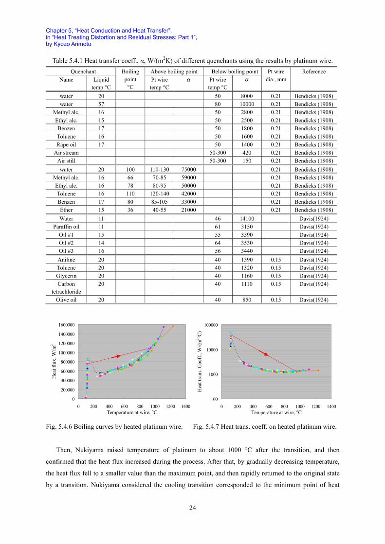
Using the experimental results with platinum wire by Benedicks (1908) and Davis (1924), Scott
(1934b) obtained heat transfer coefficients between the platinum wire and quenchants as shown in Table
5.4.1. He compared his obtained values with the case of a vertical steel plate shown in the book by
McAdams (McAdams, 1933 first edition of 1954). On the other hand, he showed that experiments by
Benedicks (1908) and Davis (1924) were clearly responding to the classified boiling and convection stages
by Lynch and Pilling (1920), based on the comparison of temperatures at the wire and boiling point of
quenchants. Therefore, at this point, the platinum wire method was not applicable to the vapor film stage.
Around that time, Nukiyama (1934) investigated heat transfer characteristics on the surface of electric
current heated platinum wire, 0.14 mm in diameter, in water at 100 °C. Heat flux at the surface was
increased rapidly by rising the temperature, and then a transition phenomenon to the state at a temperature
of 900 °C, shown as the red arrow, was appeared when heating it to the temperature of about 115 °C, as
shown in Fig. 5.4.6. In addition, this figure was redrawn by the author after converting units of the heat flux
in the original figure. It was revealed that maximum heat flux was produced at the point before this
transition, while the results observed that the platinum wire was covered with a vapor film by separating it
from water at the state after the transition. In addition, this kind of relation between the heat flux and the
temperature is called as the boiling curve. Incidentally, the author created the diagram for the temperature
dependence of heat transfer coefficients by converting from the boiling curve as shown in Fig. 5.4.7 for
reference.
Chapter 5, “Heat Conduction and Heat Transfer”, in “Heat Treating Distortion and Residual Stresses: Part 1”, by Kyozo Arimoto
24
Table 5.4.1 Heat transfer coeff., α, W/(m2K) of different quenchants using the results by platinum wire. Quenchant Above boiling point Below boiling point
0 200 400 600 800 1000 1200 1400Temperature at wire, °C
Hea
t flu
x, W
/m2
100
1000
10000
100000
0 200 400 600 800 1000 1200 1400Temperature at wire, °C
Hea
t tra
ns. C
oeff
., W
/(m2 °C
)
Fig. 5.4.6 Boiling curves by heated platinum wire. Fig. 5.4.7 Heat trans. coeff. on heated platinum wire.
Then, Nukiyama raised temperature of platinum to about 1000 °C after the transition, and then
confirmed that the heat flux increased during the process. After that, by gradually decreasing temperature,
the heat flux fell to a smaller value than the maximum point, and then rapidly returned to the original state
by a transition. Nukiyama considered the cooling transition corresponded to the minimum point of heat
Chapter 5, “Heat Conduction and Heat Transfer”, in “Heat Treating Distortion and Residual Stresses: Part 1”, by Kyozo Arimoto
25
transfer. In addition, he pointed out an analogy between a behavior of platinum wire during a temperature
drop and a cooling phenomenon during quenching. In addition, the study by Nukiyama was introduced as a
pioneering work in the field of boiling heat transfer over the textbooks on heat transfer (Jakob, 1949 &
1957; McAdams, 1954; Gröber, Erk and Griugull, 1961; Katto, 1964; Lienhard and Lienhard, 2011).
Studies on the boiling phenomena using the platinum wire can be characterized by examining heat
transfer properties of quenchants by a heated probe. After that, by obtaining pool boiling curves of
quenchants with not only a wire but also other shapes of the probe, which were made of platinum as well as
other metals, researches in this field had been developed rapidly (Jakob, 1949 & 1957; McAdams, 1954;
Gröber, Erk and Griugull, 1961; Katto, 1964; Lienhard and Lienhard, 2011).
In more recent years, Thompson and Bergles (1970) conducted a study to confirm the analogy between
pool boiling and quenching, which was suggested by Nukiyama. They provided a copper pipes for a heated
probe of pool boiling, and specified its dimensions to 0.5 in (12.7 mm) in diameter and 0.02 in (0.5 mm) in
thickness for Freon-113 and distilled water, and the same outer diameter and 0.425 in (10.8 mm) in inner
diameter for liquid nitrogen. On the other hand, the quenching test using a copper cylindrical probe, 0.5 in
(12.7 mm) in diameter and 3 in (76.2 mm) in length, or a toroidal probe, 0.5 in (12.7 mm) in diameter and
5.5 in (139.7 mm) in toroidal diameter. Heat flux - temperature curves of Freon-113, distilled water and
liquid nitrogen, which were obtained from both of steady pool boiling and quenching tests, were compared,
and then it was suggested that the results have a practical implication although an agreement was not
enough.
10000
100000
1000000
1 10 100 1000
Surface temp.-liquid temp, °C
Hea
t flu
x, W
/m2
QuenchingPool boiling
sub 0 °C sub 10 °C
sub 20 °C
sub 30 °C
sub 40 °C
100
1000
10000
100000
0 50 100 150 200 250
Surface temp. °C
Hea
t tra
ns. c
oeff
., W
/(m2 °C
)
Quenching
Pool boiling
sub 0 °Csub 10 °C
sub 20 °C
sub 30 °C
sub 40 °C
Fig. 5.4.8 Boiling curves of ethyl alcohol. Fig. 5.4.9 Heat trans. coeff. curves of ethyl alcohol.
Research on the above analogy was performed by Tachibana and Enya (1972) by a different kind of
laboratory equipments using Freon-113 and ethyl alcohol. Steady-state pool boiling curves were obtained
during heating quenchants through a 0.1 mm thick copper sheet. On the other hand, cooling curves were
measured using a copper disc probe, 50 mm in diameter and 2 mm in thickness, during cooling on a single
side, which provided a thermocouple on the opposite side of the disc. In addition, copper or mild steel
cylindrical probes, 8 mm in diameter and 70 mm in length, were used for comparison. By comparing
between pool boiling and quenching curves of Freon-113 and ethyl alcohol, they concluded that the steady
pool boiling data is used reasonably as a first approximation of the heat transfer characteristics during
Chapter 5, “Heat Conduction and Heat Transfer”, in “Heat Treating Distortion and Residual Stresses: Part 1”, by Kyozo Arimoto
26
quenching. The author created Fig. 5.4.8 by converting the units of the boiling curve of ethyl alcohol in
their original figure. In addition, since the report noted the saturation temperature of ethyl alcohol is
78.4 °C, the boiling curves could convert to the heat transfer coefficient - temperature curves as shown in
Fig 5.4.9. 5.4.4 Prediction of HTC based on lumped heat capacity method
A method to obtain surface heat transfer coefficients (HTC) from cooling curves measured in a silver
sphere probe was developed by Rose (1940). In this technique, temperature within the probe can be
assumed to be uniform at any point during cooling process because of the high thermal conductivity of
silver. Then the relative amount of heat contained in the probe, QV, is as follows:
V pQ C VTρ= (5.4.3)
where T is the uniform temperature of the probe, Cp and ρ are specific heat and density of silver, and V is
the volume of a sphere.
On the other hand, since the heat flux on a probe surface, qS, is obtained from the boundary condition in
equation (5.2.9), which includes the heat transfer coefficient α, the total heat flowed out from the surface of a probe per unit time, SQ , is:
( )S eQ S T Tα= − (5.4.4)
where Te is the temperature of a quenchant, and S is the total surface area of a probe. Since SQ obtained from Eq. (5.4.4) is equal to the time change of the heat in a probe, QV, in Eq.
(5.4.3), the following relation is derived.
( )= ( )p
e
d C TV Sh T T
dtρ
− (5.4.5)
By ignoring the temperature dependence of the density and specific heat, the heat transfer coefficient, α, is
obtained as:
=( )
p
e
C VdTdt S T T
ρα
− (5.4.6)
from the Eq. (5.4.5). The above approach to determine the heat transfer coefficient is generally called as the
lumped heat capacity method (Totten et al., 1993).
As already mentioned, Rose (1940) measured cooling curves at the center of the 20 mm diameter silver
sphere immersed in quenchants with a flow rate of about 25cm/s or sometimes 10 cm/s. Then, he applied
the lumped heat capacity method to the cooling curves for obtaining heat transfer coefficients, and then
made a table to compare with those by other researchers. The author reconstituted a part of the data in the
Rose’s table as shown in Table 5.4.2. Here, heat transfer coefficients representing the vapor film, boiling
and convection stages were shown after converting the unit from kcal/(m2h°C) to W/(m2K). Meanwhile,
Rose described, the data in the original table by Engel (1931) was obtained from the sphere probe, its
Chapter 5, “Heat Conduction and Heat Transfer”, in “Heat Treating Distortion and Residual Stresses: Part 1”, by Kyozo Arimoto
27
diameter were 4 or 7 mm, corresponded to the materials, Cr-Ni steel or silver, respectively.
Table 5.4.2 Heat transfer coeff., α, W/(m2K) of different quenchants using lumped heat capacity method. Quenchant Vapor blanket Nucleate boiling Convection
Name Temp °C
Cooling Rate cm/s
Temp °C
α Temp°C
α Temp °C
α Probe Reference
water 20–25 moderate 38–35 3500 32%Ni Scott (1934a)water 20–25 moderate 39 6050 1%C Scott (1934a)water 18 moderate 720 6300 550 10100 Cr–Ni Engel (1931)water 15.5 moderate 720 3490 200 25000 Ag Engel (1931)water 20 25 700 3110 500 12600 90 2440 Ag Rose (1940) water 8 10 700 1270 300 6050 Ag Rose (1940)
rape oil 20 moderate 720 2110 550 2790 300 768 Cr–Ni Engel (1931)rape oil 20 moderate 720 1980 550 3490 200 512 Ag Engel (1931)rape oil 20 25 700 1690 500 3660 200 488 Ag Rose (1940)
oil 20–25 moderate 178–57 451–394 32%Ni Scott (1934a)oil 20–25 moderate 58 512 1%C Scott (1934a)
oil heavy 20 moderate 720 843 600 3190 300–200 670–372 Cr–Ni Engel (1931)oil light 20 moderate 720 500 500 2970 200 744 Cr–Ni Engel (1931)
oil heavy 20 moderate 720 686 500 3490 200 599 Ag Engel (1931)oil heavy 20 25 700 1420 550 3020 300–200 314–244 Ag Rose (1940) oil light 20 25 700 779 450 3260 300–200 477–244 Ag Rose (1940)
air 20–25 non 780–75 108–19 32%Ni Scott (1934b)air 20–25 non 62 19 1%C Scott (1934b)air 20 non 720–200 74–17 Ag Engel (1931)air 20 non 700–200 49–33 Ag Rose (1940) air 20 stream 720–200 307–149 Cr–Ni Engel (1931)air 20 stream 700–200 465–256 Ag Rose (1940)
Krainer and Swoboda (1944) obtained temperature curves of the heat transfer coefficient for five
different kinds of quenching oils and the two different temperature waters based on the Rose’s study. After
converting the unit of heat transfer coefficients in the original figure in their paper to the SI system,
Fig.5.4.10 was made by the author. As a result, a temperature dependence of heat transfer coefficients was
shown more clearly than the form depicted in Table 5.4.2.
100
1000
10000
100000
0 200 400 600 800Temperature, °C
Hea
t tra
nsfe
r coe
ff, W
/(m2 °C
) Oil A Oil B Oil COil D Oil E Water 20°CWater 60°C
Fig. 5.4.10 Temperature curves of heat transfer coefficients by Krainer and Swoboda.
Chapter 5, “Heat Conduction and Heat Transfer”, in “Heat Treating Distortion and Residual Stresses: Part 1”, by Kyozo Arimoto
28
Jones and Pumphrey (1947), as already mentioned, obtained cooling curves of waters and oils using a
silver cylinder, 3/4 in (19 mm) in diameter and 3 in (76 mm) in length. Then by applying the lumped heat
capacity method to the data, they got and showed temperature curves of the quenching constant h, not the
heat transfer coefficient, for one type of oil and a water about 80 °C.
A method which was similar to the lumped heat capacity method was applied by Shyne and Sinnott
(1952) to a quenching phenomenon in KNO3–NaNO2 salt cooling, in spite of a significant temperature
gradient in a probe. A cylindrical probe made of the 430 stainless steel, 1 in (25.4 mm) in diameter and 6 in
(152 mm) in length, was heated to 845 °C, and then immersed in the salt that is set to temperature levels
between 195 and 385 °C. Cooling curves are measured at the center and on the surface of the probe, and
their average temperature was considered as the probe temperature for applying the lumped heat capacity
method. A heat lost from the probe was determined by multiplying a mass and a specific heat of the probe
to the temperature difference between initial and current probe temperatures. This time changes of the heat
correspond to the left side of Eq. (5.4.5). A heat transfer coefficient, α, was calculated by Eq. (5.4.6) in
which measured surface temperature of the probe was specified as the temperature, T, at the right side of
the equation.
For obtaining heat transfer coefficients of spray and air blast cooling, the lumped heat capacity method
was applied by Shimada et al. (1976) to cooling curves measured from a silver disc probe. Dimensions of
the silver discs were 2 mm in thickness and 20, 30 or 40 mm in diameter, which were provided a
thermocouple at its center. Heat transfer coefficients of the air blast cooling did not show almost a
temperature dependence, and had a value of about 230 W/(m2K). In contrast, the dependence appeared in
the case of spray cooling, as similar to normal water quenching, and the heat transfer coefficients tended to
increase after temperature decreasing less than 300 °C. Values of heat transfer coefficients were outlined, as
350 W/(m2K) in the high temperature range, and 3500 W/(m2K) in the vicinity of the peak position of
Fig. 5.4.14 Heat trans. coeff. by Tensi and Steffen Fig. 5.4.15 Heat trans. coeff. by Liscic.
Liscic (1992) devised a method to obtain a surface heat flux based on a difference of the cooling curves
measured from thermocouples at the surface and 1.5 mm in depth from the surface in an austenitic stainless
steel (AISI 304) cylindrical probe, 50 mm in diameter and 200 mm in length. This probe has a structure that
can be installed internal thermocouples within a tolerance of less than ± 0.025 mm. Liscic and Filetin
(2011) applied the above apparatus to a low viscous accelerated quenching oil of 50 °C with medium
agitation, and obtained a temperature curve of heat transfer coefficients as shown in Fig. 5.4.15.
Segerberg and Bodin (1992) obtained heat transfer coefficients at different surface positions of
quenched cylinders and rings into still oils at 70 °C as shown in Fig. 5.4.16 and Fig. 5.4.17, respectively.
Cooling curves of cylinders, 30 mm in diameter and 90 mm in length, were measured at near the upper
(point 5), lower (point 6) and longitudinal surfaces (point 1-4). A ring, 110 mm in outer diameter, 70 mm in
inner diameter and 30 mm in height, was quenched in a horizontal position, and cooling curves were
measured at near the top, bottom and side surfaces of the probes. Another ring, 110 mm in outer diameter,
35 mm in inner diameter and 10 mm in height, was quenched in horizontal and vertical positions. The
obtained heat transfer coefficient curves of these rings described that the positioning contributes to the
characteristics of heat transfer coefficients, as shown in Fig. 5.4.18.
Chapter 5, “Heat Conduction and Heat Transfer”, in “Heat Treating Distortion and Residual Stresses: Part 1”, by Kyozo Arimoto
32
0
1000
2000
3000
4000
5000
6000
0 200 400 600 800 1000
Surface tempearture, °C
Hea
t tra
ns. c
oeff
., W
/(m2 °C
) Point 1 Point 2Point 3 Point 4Point 5 Point 6
0
1000
2000
3000
4000
5000
6000
0 200 400 600 800 1000
Surface tempearture, °C
Hea
t tra
ns. c
oeff
., W
/(m2 °C
) Point 1Point 2Point 3Point 4
Fig. 5.4.16 Heat trans. coeff. of a cylinder. Fig. 5.4.17 Heat trans. coeff. of a ring.
0
1000
2000
3000
4000
5000
6000
0 200 400 600 800 1000
Surface tempearture, °C
Hea
t tra
ns. c
oeff
., W
/(m2 °C
) Point 1Point 2Point 3
0
1000
2000
3000
4000
5000
6000
0 200 400 600 800 1000
Surface tempearture, °C
Hea
t tra
ns. c
oeff
., W
/(m2 °C
) Point 1Point 2Point 3
(a) Horizontal position. (b) Vertical position.
Fig. 5.4.18 Heat transfer coefficient of ring.
0
200
400
600
800
1000
1200
0 10 20 30 40 50 60
Time, s
Tem
pera
ture
, °C
D=130 x L=390D=30 x L=90D=12.5 x L=60
0
1000
2000
3000
4000
5000
6000
0 200 400 600 800 1000
Surface tempearture, °C
Hea
t tra
ns. c
oeff
., W
/(m2 °C
) D=130 x L=390D=30 x L=90D=12.5 x L=60
(a) Cooling curves. (b) Heat trans. coeff.
Fig. 5.4.19 Heat transfer coefficient of cyrinders.
In addition, Segerberg and Bodin quenched Inconel 600 cylinders with different diameters into the
same quenching oil as the above, and obtained cooling curves with different shapes apparently, except only
the 12.5 mm diameter cylinder was measured at its center, as shown in Fig. 5.4.19 (a). Then, they
concluded that since the curves of heat transfer coefficient estimated based on the results agreed well each
other as shown in Fig 5.4.19 (b), the value from the smallest diameter probe can be applied to larger
Chapter 5, “Heat Conduction and Heat Transfer”, in “Heat Treating Distortion and Residual Stresses: Part 1”, by Kyozo Arimoto
33
diameter cases. It was also described that a heat transfer coefficient by a silver probe was consistent with
the results of the Inconel probe. In addition, the heat transfer coefficients in their paper were estimated
based on cooling curves and numerical calculations of heat conduction problems.
Using quenching test results from a hollow cylinder, 60 mm in outer diameter, 30 mm in inner diameter
and 60 mm in height, made of Cr-Ni steel, X 6 CrNiTi18 19, Tensi and Lainer (1996) determined heat
transfer coefficients on the inner and outer surfaces. In this study, based on the calculation of
one-dimensional heat conduction and using cooling curves obtained at three points of probe, heat transfer
coefficients were estimated by trial and error. In addition, the quenchant was oil at 60 °C, which was tested
under still and 2 kinds of agitation conditions.
Laumen et al. (1997) measured cooling curves at the center and a point near the surface, which is the
position of 0.9R, R: radius, of an austenitic stainless steel cylinder, 28 mm in diameter and 112 mm in
length, in order to determine heat transfer characteristics of a gas cooling. An actual temperature of the gas
was measured at the gas entry and exit in a furnace. The radial temperature distribution of the probe was
obtained by the finite deference method under a condition to match a calculated value at 0.9R with the
measurement. Using the heat flux calculated by a similar manner to Liscic (1992) from the measured
temperature at 0.9R and estimated surface temperature, and then heat transfer coefficients were obtained by
applying the averaged of the measured gas temperatures additionally to Eq. (5.4.4). The heat transfer
coefficient of the 10bar H2–N2 gas mixture, 0-100 % H2, were obtained as values in the range of from 400
to 600 W/(m2K).
5.4.6 Prediction of HTC based on inverse analysis
As already noted, cooling curves obtained from low mass probes made of high thermal conductivity metals
such as silver, gold and platinum can be used to predict heat transfer coefficients (HTC) simply by using
the lumped heat capacity method. On the other hand, for conditions not applicable to this method, the
inverse heat transfer analysis technique (Beck et al., 1985; Beck and Osman, 1992) has been developed.
This can predict heat transfer coefficients for temperature dependent phenomena of the heat conduction.
(1) One dimensional problem
Wallis (1989) obtained temperature curves of heat transfer coefficients on upper and lower surfaces of the
Alloy 718 disc during quenching it horizontally, using the CONTA program for one-dimensional inverse
analysis, as shown in Fig. 5.4.20 (a). Units of temperature and heat transfer coefficient in this figure were
converted from the original figure by the author. This inverse calculation used cooling curves measured at
several thermocouples, the number of which was not stated in the report, located in the central part and
along the thickness direction of the disc. Meanwhile, temperature curves of the heat transfer coefficients
were obtained during quenching the disc vertically, and then the results are shown in Fig. 5.4.20 (b) for
comparison with the case of quenching in the horizontal position.
Chapter 5, “Heat Conduction and Heat Transfer”, in “Heat Treating Distortion and Residual Stresses: Part 1”, by Kyozo Arimoto
34
0
1000
2000
3000
0 200 400 600 800 1000 1200 1400
Surface tempearture, °C
Hea
t tra
ns. c
oeff
., W
/(m2 °C
) Top surfaceBottom surface
0
1000
2000
3000
0 200 400 600 800 1000 1200 1400
Surface tempearture, °C
Hea
t tra
ns. c
oeff
., W
/(m2 °C
) VerticalHorizontal (top)
(a) Top and bottom surfaces in horizontal position. (b) Vertical and horizontal positions.
Fig. 5.4.20 Predicted heat transfer coefficient of disc quenched into oil.
Hernandez-Morales et al. (1992) predicted heat transfer coefficients by applying the CONTA program
for one-dimensional inverse analysis, using cooling curves obtained from steel disc probes. Discs, 200 mm
in diameter and 20 mm in thickness, were made of stainless or mild steels. Thermocouples were provided at
only one point located 1.4 mm in depth from the surface on a single side of the disc. Using water, brine, oil
and air as quenchants, discs were quenched vertically. Temperature curves of heat transfer coefficients were
reported for various conditions, some of which were compared with the results in literatures.
Felde et al. (2005) applied a one-dimensional inverse problem analysis to cooling curves obtained at the
center of the Inconell 600 cylindrical probe, 12.5 mm in diameter, for predicting temperature curves of heat
transfer coefficients. On the other hand, Felde et al. (2009) used the same method for cooling curves
obtained from the JIS K 2242 silver probe. Obtained temperature curves of heat transfer coefficients were
confirmed to be almost identical to those calculated from the lumped heat capacity method.
(2) Two dimensional problem
Trujillo and Wallis (1989) investigated heat transfer characteristics during oil quenching an Alloy 718 disc
using the INTEMP program for two-dimensional axisymmetric inverse problem analysis. Cooling curves
was measured at several points within the disc, 10.5 in (266.7 mm) in diameter and 2.75 in (69.9 mm) in
thickness, during quenching it horizontally from 2150 °F (1177 ° C). Then applying the inverse analysis to
this result, heat flux changes were obtained in 7 ranges on surfaces in an axisymmetric cross section.
Heat transfer phenomena in Ni-based super alloy rings quenched in forced air and oil were examined by
Ramakrishnan (1992) using the QUENCH2D program for two-dimensional axisymmetric inverse problems.
Dimensions of the ring were 355.6 mm in outer diameter, 76.2 mm in inner diameter and 69.9 mm in height.
Probes were heated to 1149 °C, and then were quenched horizontally into oils in the range of 21 to 24 °C
temperature with agitation. In the case of air cooling, the heating was similar to the oil; on the other hand,
cooling was done by high-speed airflow on the top and bottom surfaces of the ring simultaneously.
Temperature curves of heat fluxes on ring surfaces for oil quenching and air cooling were obtained as
shown in Fig. 5.4.21(a) and Fig. 5.4.22(a), respectively, by applying QUENCH2D to cooling curves
Chapter 5, “Heat Conduction and Heat Transfer”, in “Heat Treating Distortion and Residual Stresses: Part 1”, by Kyozo Arimoto
35
measured at 13 thermocouples installed inside the ring. The author converted these to heat transfer
coefficients as shown in Fig. 5.4.21(b) and Fig. 5.4.22(b), respectively. In addition, these curves are
corresponding to the four sides in the cross-section of the ring, upper, lower, inner and outer surfaces.
0
1000000
2000000
3000000
4000000
5000000
0 200 400 600 800 1000 1200
Surface tempearture, °C
Hea
t flu
x, W
/m2
I. D. & O. D. surfacesTop surfaceBottom surface
0
1000
2000
3000
4000
5000
6000
7000
8000
0 200 400 600 800 1000 1200
Surface tempearture, °CH
eat t
rans
. coe
ff.,
W/(m
2 °C) I. D. & O. D. surfaces
Top surfaceBottom surface
(a) Heat flux. (b) Heat transfer coefficient.
Fig. 5.4.21 Predicted heat transfer characteristics of ring quenched into oil.
0
100000
200000
300000
400000
500000
600000
0 200 400 600 800 1000 1200
Surface tempearture, °C
Hea
t flu
x, W
/m2
I. D. surfaceTop & Bottom surfacesO. D. surface
0
100
200
300
400
500
600
0 200 400 600 800 1000 1200
Surface tempearture, °C
Hea
t tra
ns. c
oeff
., W
/(m2 °C
) I. D. & O. D. surfaceTop surfaceBottom surface
(a) Heat flux. (b) Heat transfer coefficient.
Fig. 5.4.22 Predicted heat transfer characteristics of ring cooled by air.
Sugianto et al. (2009) predicted heat transfer coefficients in different surface regions of a cylindrical
stainless steel probe quenched into water using inverse analysis programs for axisymmetric
two-dimensional problems. 6 thermocouples were provided at the center, at the upper and lower surface
points, and at 3 points on the side in the cylinder, 20 mm in diameter and 60 mm in length. Three
conditions of water quenching were still, and the 0.3 and 0.7 m/s agitation. Inverse calculations were
attempted by two methods, one uses heat transfer coefficients of silver probe as initial values and another is
software included in a commercial heat treating simulation code. Results from the still quench condition,
which was reported overall, described that the predictions by the method using initial values of the silver
probe agreed better with the experiments.
Chapter 5, “Heat Conduction and Heat Transfer”, in “Heat Treating Distortion and Residual Stresses: Part 1”, by Kyozo Arimoto
36
5.4.7 Prediction of HTC based on CFD
The fluid flow simulation, which is also called as computational fluid dynamics (CFD), has recently
become popular in a variety of fields. Although this is to be applied for quenchant flows, in general, its
major role is for the salt or gas quenching.
(1) Salt bath quenching
The fluid flow analysis was applied to the salt bath quenching by Shick et al. (1996). In this study, first, the
physical properties of the salt, such as viscosity, density, specific heat and thermal conductivity were
reviewed. Cooling curves at the center of 1/4, 1/2, 1, 2 and 3 in diameter cylindrical probes made of
stainless steel predicted by a flow analysis were compared with those described in past literatures. The 1/4
in diameter probes was quenched from 871 °C into the 258 °C salt bath. Meanwhile, the 1/2 in diameter
and from 1 to 3 in diameter probes were quenched from 850 °C into 220 °C and from 900 °C into 200 °C,
respectively. The predicted and experimental results agreed well.
On the other hand, the CFD commercial code (STAR-CD) was applied to the fluid flow analysis of a
steel ring during salt bath quenching. The ring, 56.7 mm in outer diameter, 35.3 mm in inner diameter and
21.0 mm in height, the upper surface of which is connected to the small ring, the same inner diameter, 43.3
mm in outside diameter and 3mm in height. The results of the fluid flow analysis estimated temperature
curves of heat transfer coefficients on the four sides of the ring in the cross section as shown in Fig. 5.4.23.
0
1000
2000
3000
4000
5000
6000
7000
0 200 400 600 800 1000
Surface tempearture, °C
Hea
t tra
ns. c
oeff
., W
/(m2 °C
) I. D. surfaceTop surfaceO. D. surfaceI. D. surface
Fig. 5.4.23 Predicted heat transfer coefficients of ring cooled in a salt bath.
(2) Gas quenching
Studies on a gas quenching by using the CFD software, ANSYS CFX, was reported by Macchion (2005).
First, he summarized typical features and geometries of furnaces for the gas quenching, flow characteristics
of pure and mixed gases, and turbulence models. As a matter of basic validation for CFD, wind tunnel
experiments on cylinders (Wiberg, 2004), 150 mm in diameter and 300 mm in length, was applied. It was
identified that surface heat transfer characteristics can be predicted well, when cooling the cylinder by a
flow in the axial direction. Next, axial direction flows around cylinders, 28 mm in diameter and 110 mm in
length, were predicted, and surface temperature distributions at a cylinder were shown. Furthermore, it was
Chapter 5, “Heat Conduction and Heat Transfer”, in “Heat Treating Distortion and Residual Stresses: Part 1”, by Kyozo Arimoto
37
made clear that different parts of a quenching rack, for example, a rod or a plate, affected flow conditions.
Subsequently, impacts of different heat transfer from gas composition were examined by CFD. In addition,
the CFD and measured results of flow rates inside the furnace were compared when it was actually empty.
Applying CFD to flows around the cylinders inserted into a furnace, the results were illustrated as
distributions of the heat transfer coefficients obtained in a typical cylinder. How differences of furnace and
duct shapes affect the flow was investigated by CFD.
Like Macchion’s studies, Fritsching and Schmidt (2007) performed a comprehensive work on flow
phenomena in the gas quenching, and proposed that phenomena could be modeled in a phased manner as
macro, meso and micro scales. A macro scale model corresponds to one focused on the upstream flow of a
furnace. A meso scale model deals with a flow state in a furnace with several components. On the other
hand, a micro scale model is used to study flow phenomena around individual parts. Examples in
comparison between simulation and experiment were shown in the each scale. In the case of micro-scale, a
comparison of the heat transfer characteristics of part surfaces was reported.
For simulating a flow around a nickel cylinder in an experimental furnace for gas quenching, Douce et
al. (2005) applied FLUENT, as the CFD software. The cylinder, 15 mm in diameter and 80 mm in length,
was placed vertically, and measured a phenomenon around it due to a fluid flow from the top by the PIV
(Particle Image Velocimetry). A simulation by FLUENT was performed for this flow condition, which was
compared with an experimental velocity distribution. In addition, heat transfer coefficients were estimated
based on the flow information, which were used for a distortion simulation.
A nitrogen flow due to gas jet nozzles from four directions, for cooling an austenitic stainless steel
cylinder, was analyzed by Frerichs (2004) using FLUENT. The velocity of the gas at the nozzle exit was
from 100 to 255 m/s. As a result, heat transfer coefficient distributions were obtained on the surfaces of the
cylinder. Heat transfer analysis performed based on these data showed that simulated cooling curves agreed
well with experiments at the center and at points on the surface of the cylinder.
On the other hand, Stratton (2007) applied FLUENT to nitrogen gas flows, induced from a multiple jet
nozzle, 100 m/s in velocity, for cooling a steel disc. Heat transfer coefficients estimated based on the results
were applied to heat conduction analysis of the disc, and a simulated cooling rate at a point was compared
with an experimental result.
(3) Liquid quenching
CFD has been attempted to apply to flow simulations induced even by liquid quenching. In these cases,
boiling phenomena of liquid quenchants are basically not considered.
Ohki (2001) applied CFD to cooling by oil jets for inner and outer diameter surfaces of a ring, and then
estimated heat transfer coefficients by referencing flow velocities around them. Predicted cooling curves at
several points of the ring cross section based on the obtained heat transfer coefficients were compared with
the experiments.
Kumar et al. (2007) applied FLUENT to a flow around pinion gears on a rack during oil quenching. In
addition, a shape before gear cutting was used for the modeling of gear.
Chapter 5, “Heat Conduction and Heat Transfer”, in “Heat Treating Distortion and Residual Stresses: Part 1”, by Kyozo Arimoto
38
To optimize a flow in a quenching oil path of a press quenching apparatus for a ring gear, Schüttenberg
(2007) used CFD. Dimensions of the ring gear were 220 mm in outer diameter, 132 mm in inner diameter
and 32 mm in height. Heat transfer coefficients on surfaces of the gear were estimated from the results by
CFD.
There are few theoretical studies to obtain heat transfer coefficients in a two-phase flow, gas and liquid,
during quenching. The research by Yamagami (2003) found by the author simulated a cooling phenomenon
by a water jet on a high temperatures stainless plate using CFD included a function of fluid phase change.
Also surface heat transfer coefficients were estimated by using an inverse analysis based on temperatures in
the steel plate.
5.4.8 Outlook on deriving heat transfer coefficients for heat treatment simulation
Ideally, if a coupling simulation is applied to both phenomena in a heat treated object and a flow around it,
it is not necessary to specify heat transfer coefficients for its model. However, at present, these cases to
which such a simulation can be applied are very limited.
Heat transfer analysis in the heat treatment simulation needs to set heat transfer coefficients on surfaces
of parts. As already mentioned, some probes to obtain cooling curves and cooling rate curves were
developed to understand the cooling power of quenchants, and then national standards and even
international standards were established for the system (Totten, Tensi and Liscic, 1997). The specific
cooling curves obtained from the individual probes can be used to make heat transfer coefficients by a
lumped heat capacity method or an inverse analysis method. These coefficients may be useful for
simulating practical problems as the first approximation.
However, since these coefficients were obtained in terms of individual conditions, a large discrepancy
with a reality may be made. For example, it is known the characteristic temperature of the probes depends
on the type of metal. That is, Narazaki et al. (2002) noted that stainless steel probe showed the highest
characteristics temperatures in oil quenching, and Ni and silver were the second and third, respectively,
based on shapes of the temperature curves of the heat transfer coefficients. Beck and Moreaux (1992) also
reported that the material dependence of the characteristic temperature could also be seen in the
relationship between heat flux and surface temperature in 100 °C water quenching of Ni, Al and silver
probes.
In practice, it is believed that a good approach for estimating heat transfer coefficients close to reality is
need by correcting the first approximation data obtained from the probes are by some approaches. The
following gives an outlook how the data are collected and corrected.
(1) Collection of first approximation data
Cooling curves obtained from the standard measuring devices for the cooling power have provided heat
transfer coefficients by a lumped heat capacity method or an inverse calculation, which were reported in
literatures. These data are the first approximations, however may be effective to be used as is for practical
purpose. Therefore, their database is significant by collecting from literature and new experimant.
Chapter 5, “Heat Conduction and Heat Transfer”, in “Heat Treating Distortion and Residual Stresses: Part 1”, by Kyozo Arimoto
39
Meanwhile, Peter (1949, 1950) reported a number of cooling rate curves, which can be converted into
temperature curves of heat transfer coefficients using a lumped heat capacity method. It is considered that
the same kinds of data as Peter’s are present. These data may be useful for making a database of
temperature curves of heat transfer coefficients with the original data.
On the other hand, heat transfer coefficients during cooling or in steady state, which were reported as
empirical formulas, should be organized after clarifying the scope of these applications.
(2) Correction methods on first approximation data
In order to correct the approximate heat transfer coefficients more realistically, it is necessary to clarify the
characteristics of the heat transfer at different locations on surfaces of simple shape components, such as
cylinders, discs and rings in typical quenching conditions. This attempt was performed by Bodin and
Segerberg (1992) as already mentioned. Also Trujillo and Wallis (1989), Ramakrishnan (1992) and
Sugianto et al. (2009) worked on the same theme using two-dimensional inverse analysis software for some
limited cases. These kinds of studies should be performed more precisely and systematically.
Heat transfer characteristics at different locations on part surfaces, especially in case of the liquid
quenchants, may be confirmed based on a collapse of vapor film, which corresponds to the end of the vapor
film stage. This collapse in a simple shape probe such as sphere and cylinder was revealed by visualization
experiments. For example, Tensi (1992a) showed it in the cases of quenching Cr-Ni steel cylinders, 25 mm
in diameter and 100 mm in length, and triangular prism, 15×15×45 mm, from 860 °C into 35 °C distilled
water. In the case of a triangular prism, boundary curves between vapor film and wetted parts were clearly
photographed. Above systematic studies of positions dependences on the heat transfer should accompany
visualization experiments on the vapor film collapse.
In addition, there are questions how heat transfer characteristics are affected by part positions on a rack
and also quenchant agitations. We will find the correction methods based on studies using experimental and
simulation works steadily.
5.5 Temperature recovery and inverse hardening phenomena Descriptions on the heat conduction in a solid and the surface heat transfer have been terminated generally
before this section, while the phase transformation has been already expressed in Chapter 3. Therefore,
simulation examples on a phenomenon due to remarkably both heat conduction and phase transformation
can be introduced here. That is a temperature recovery in a cooling curve during phase transformation by a
heat generation, which may induce an inverse hardening phenomenon additionally.
5.5.1 Temperature recovery phenomenon
When quenching a cylindrical steel specimen slowly, it has long been known that a temperature recovery
called as recalescence phenomenon may occurs (Bain and Paxton, 1966). Takeo et al. (1974) quenched
0.84 %C-0.68% Mn steel cylinders with 11 different diameters, the range from 3.5 to 25 mm, into boiling
water, and then measured cooling curves at its center. As a result, temperature recovery phenomena were
Chapter 5, “Heat Conduction and Heat Transfer”, in “Heat Treating Distortion and Residual Stresses: Part 1”, by Kyozo Arimoto
40
found in cooling curves from cylinders of more than 4.5 mm in diameter. In addition, this experiment was
conducted in relation to a study on a patenting process of steel wires. As for the boiling water quenching,
heat transfer coefficients were evaluated by Iwata et al. (1980) based on both the experimental and
theoretical procedures.
Experiments by Takeo et al. for the 5.5, 8.5, 13 and 25 mm diameter steel cylinders were simulated by
Agarwal et al. (1981), and the temperature recovery generation was confirmed under the same experimental
conditions. Simulated results of an air-cooled steel cylinder, 12 mm in diameter, showed a temperature
recovery as well as an associated significant delay in the progress of the diffusion transformation at the
center than near the surface. These experiments by Takeo et al. were also simulated by Arimoto et al.
(1998), and it was confirmed simulated and experimental cooling curves agreed as shown in Fig. 5.5.1. In
this simulation, a TTT diagram was used after time-shifting the data for 1080 steel by US Steel (1951) as
shown in Fig 3.3.3 in Section 3.3.2, and data of the enthalpy of phase transformation was referred as 75.8
kJ/kg, which was derived from measurements by Kramer (1958). In addition, Fig. 5.5.1 depicted a
simulated cooling curve using 83 kJ/kg as the enthalpy temporarily for reference.
0 20 40 60 80 100
500
600
700
800
900
Time, s
Tem
pera
ture
, C
Measured 8.5mm 13mm25mm
Calculated 75.8kJ/kg 83kJ/kg
Fig. 5.5.1 Temperature recovery phenomenon at center of 12 mm dia. eutectoid steel
cylinder during 100°C water quenching.
Otsuka et al. (1987) cooled a 1% Ni eutectoid steel cylinder, 3 mm in diameter and 10 mm in length,
under about 10–6 Torr in a temperature – dilatation measuring apparatus, Formastor-F, after holding it for 15
min at 1000 °C. An obtained cooling curve showed a temperature recovery, which was predicted by
considering a generated heat due to a phase transformation by the heat conduction analysis.
5.5.2 Inverse hardening phenomena
After oil quenching of bearing races and rollers, an inverse hardening phenomenon had been found in the
parts in the past. Tamura and Shimizu (1975) discussed that this phenomenon was produced by residual
vapor films at some locations on surfaces during cooling. Then, they simulated experimentally this cooling
delay due to the vapor films as air-cooling, and then defined a test using cylindrical specimens of simple
Chapter 5, “Heat Conduction and Heat Transfer”, in “Heat Treating Distortion and Residual Stresses: Part 1”, by Kyozo Arimoto
41
geometry for reproducing the phenomenon. In their experiment, SUJ2 steel cylinders with 6 different
diameters, 10, 15, 20, 25, 30 and 36 mm, were held for 20 min at 840 °C, and then finally quenched into
5% brine after air cooling for various periods.
A phenomenon in the 20 mm diameter cylinder, which was found in one of the tests by Shimizu and
Tamura, was simulated by the authors (Arimoto et al., 2000). The simulation used the TTT diagrams shown
in Fig 3.2.2 in section 3.2.5 for steel bearings, which were specified for the steels, 52100 (US Steel, 1951),
En 31 (BISRA, 1949) and 100 Cr 6 (Max Planck Institute, 1954). Changes of temperature and volume
fraction of pearlite at the center and on the surface of the specimen were obtained as shown in 5.5.2. The
cooling curve at the center showed a similar temperature recovery phenomenon as shown in Fig. 5.5.1,
while there was a delay of phase transformation progress at the center than the surface. These curves
identified the different trends derived from each the TTT diagram. By neglecting the effect of the heat
generation by phase transformation of steel 52100, the temperature recovery disappeared as shown in the
figure. In this case, progress curves of phase transformations have the same shape at the center and the
surface, that is, they are merely shifted as an interval of about 5 s. In this simulation, the enthalpy of phase
transformation was referred as 75.8 kJ/kg from the measurements by Kramer et al. (1958).
0 20 40 60 80 100550
600
650
700
750
800
850
0
0.2
0.4
0.6
0.8
1
Time, s
Tem
pera
ture
, C
Vol
ume
frac
tion
trans
form
ed
52100 En 31 100 Cr 6 52100(without
latent heat)
Temperature
Volumefraction
C
S
CS
CS
S C
C: CenterS: Surface
C
0.01 0.02 0.04 0.1600
620
640
660
680
700
dξ/dt, 1/s
Tem
pera
ture
, C
0.5
0.1
0.5
0.5
0.50.1
0.9
ξ=0.1
0.1
0.1
0.9
0.5
0.50.9
0.9
0.9
En 31 Center Surface100 Cr 6 Center Surface
0.1
0.9
Lines of (dξ/dt)ξ=0.5
52100 En 31 100 Cr 6
Locus of dξ/dt52100(with latent heat) Center Surface(without latent heat) Center Surface
0.1
0.5
0.9
Fig. 5.5.2 Predicted temperature and pearlite Fig. 5.5.3 Loci of pearlite volume fraction
volume fraction in 20 mm dia. rate at center and surface in bearing steel cylinders. 20 mm dia. bearing steel cylinders.
Based on the simulated results from the steel cylinder using the different TTT diagrams, Fig. 5.5.3
described loci of points which correspond to temperatures and transformation rates at the center and on the
surface. In the figure, curves of the relationship between temperature and transformation rate at the 50
percent transformation, shown by dotted lines, which are hereinafter simply referred to as the
transformation rate curve, are drawn for the 3 kinds of the TTT diagrams. On the other hand, loci of
temperature and transformation rate points are created by connecting points from 10 to 90% of volume
fraction with curve segments. Looking at the locus of the steel 52100, it is identified that their shapes at the
Chapter 5, “Heat Conduction and Heat Transfer”, in “Heat Treating Distortion and Residual Stresses: Part 1”, by Kyozo Arimoto
42
center and on the surface are quite different. The locus on the surface locates right than at the center, which
means the transformation rate on the surface is greater than the center; therefore, the progress of phase
transformation on the surface is faster. Incidentally, ignoring the effect of the heat generation due to phase
transformation in the 52100 steel, the loci at the center and on the surface are almost same, therefore, they
are overlaid as shown in the figure.
The point on the locus at 50 % transformation contacts inevitably the transformation rate curve of the
50 % transformation. This means that constraints are imposed on existence ranges of the locus. For
example, a comparison between En 31 and 52100 steels shows that transformation rate curve of the 50%
transformation in En 31 is located in the lower left region than that of steel 52100. Thus, the locus of En 31
is also located in the lower left region inevitably than the 52100 steel. In addition, locating in the left region
decreases overall an activity level of phase transformation, and locating in the lower region means phase
transformations occur in lower temperature.
Here, simulated results of the 52100 and 100 Cr 6 steels are compared. The transformation rate curve of
100 Cr 6 steel is located in left region than the curve of 52100 steel except the range higher than 680 °C. In
addition, the curvature of the curve is smaller than the 52100 steel. Loci shapes at the center and on the
surface in the 100 Cr 6 steel are similar, which may be contributed by the small curvature of the
transformation rate curve. Meanwhile, since the En 31 and 52100 steels have larger curvatures in the
transformation rate curve, tends are shown that loci at the center remains extremely in an area of smaller
transformation rate than the surface. This is considered that a progress of transformation at the center
decrease than the surface in the En 31 and 52100 steels.
0 20 40 60 80 100 120550
600
650
700
750
800
850
0
0.2
0.4
0.6
0.8
1
Time, s
Tem
pera
ture
, C
Pear
lite
volu
me
frac
tion
60s
70s
70s80s
90s
80s90s
100s
60s 70s 80s 90s 100s
Center
Surface
Temperature
Volumefraction
0 2 4 6 8 1020
30
40
50
60
7040s
50s60s
70s
80s
90s
100s
Depth, mm(i) Measured
Har
dnes
s, H
RC
0 2 4 6 8 10
50s
65s
80s
60s
Depth, mm(ii) Simulated 52100
70s
70s
80s
90s
75s
100s 80s with l. h. without l. h.
0 2 4 6 8 10
90s
70s
En 31 100 Cr 6
Depth, mm(iii) Simulated En31&100Cr6
60s
100s
50s
80s
Fig. 5.5.4 Predicted temperature and pearlite volume Fig. 5.5.5 Experimental and simulated
fraction in 20 mm dia. bearing steel cylinders hardness distribution in 20 mm dia. during air and brine cooling. bearing steel cylinders.
In the experiments for the inverse hardening by Shimizu and Tamura, specimens were quenched into
Chapter 5, “Heat Conduction and Heat Transfer”, in “Heat Treating Distortion and Residual Stresses: Part 1”, by Kyozo Arimoto
43
5% brine after air cooling for 60, 70, 80, 90 or 100 s. Fig. 5.5.4 shows simulated results by the authors,
which include temperature and pearlite volume fraction changes on the surface and at the center during the
two-stages cooling. In this simulation, the TTT diagram for the 52100 steel was used. As shown clearly in
the figure, temperature in the specimens decrease rapidly during the 5% brine quenching and then the
pearlite transformation on the surface is stopped almost instantly. On the other hand, pearlite transformation
in the core is stopped after some continuity.
In Fig. 5.5.5, simulated hardness distributions in the 20 mm diameter cylinder are compared with the
experimental results by Shimizu and Tamura. Shapes of the simulated hardness distributions show the
inverse phenomena, which are similar to the experiments. In addition, predicted values of hardness were
derived by the weighted mean method using the harnesses and volume fractions of each martensite and
pearlite.
Experimental hardness distributions show the inverse phenomena in the cases of the air-cooling for
from 50 to 100 s, while simulation predicted the phenomena in the cases of air cooling for from 60 to 100 s.
In addition, predicted hardness distributions have different shapes, which occurred due to the differences of
the TTT diagram for it. Incidentally, in the simulated results without heat generations due to phase
transformations using the TTT diagram of steel 52100 show the inverse hardening in cases of air-cooling
for from 60 to 75 s, which is obviously different from the experiments.
As mentioned above, the simulated results did not agree fully with the experiments. The reason is that
the TTT diagrams for the simulation did not correspond directly to the SUJ2 steel which was used for the
specimens. Since it is clear that a distinct difference in the simulated results was induced from the different
TTT diagrams, the simulation should use the TTT diagram of the SUJ2 steel used for the specimens. Other
cause of the discrepancy may be produced from the data of the phase transformation enthalpy, since the
data from the eutectic steel was used instead of the SUJ2 steel. In addition, experimental and simulated
results for the cooling processes with temperature recovery phenomena could not be directly compared,
since Shimizu and Tamura did not report their cooling curves.
Then, the authors (Arimoto et al., 2004a) reproduced experimentally the inverse hardening phenomena
using the 20 mm diameter cylindrical specimens, and confirmed to appear a similar temperature recovery in
a cooling curve as shown in Fig. 5.5.2. This experiment was simulated based on the above mentioned
approach, and then a tendency of simulated temperature changes during the temperature recovery agreed
well with the experiments. However, they did not agree precisely, since the TTT diagram was not produced
from the same grades of the actual specimen. Similarly, the exact agreement for the hardness distributions
was not obtained.
Reference Agarwal, P. K. and Brimacombe, J. K., 1981, “Mathematical Model of Heat Flow and Austenite– Pearlite Transformation in
Eutectoid Carbon Steel Rods for Wire,” Metall. Trans., Vol. 12B, pp. 121–133. Arimoto, K., Huang, D., Lambert, D. and Wu, W. T., 2000, “Computer Prediction and Evaluation of Inverse
Quench–Hardening of Steel, 20th Heat Treating Conference, ASM International, pp. 737–746. Arimoto, K., Jin, C., Tamura, S., Funatani, K. and Tajima, M., 2004a, “Verification of Inverse Quench– Hardening
Chapter 5, “Heat Conduction and Heat Transfer”, in “Heat Treating Distortion and Residual Stresses: Part 1”, by Kyozo Arimoto
44
Phenomena in Bearing Steel Specimens by Experiment and Computer Simulation,” Transactions of Materials and Heat Treatment, Vol. 25, No. 5, pp. 465–470, (14th Congress of International Federation for Heat Treatment and Surface Engineering, October 26–28, 2004, Shanghai, China)
Arimoto, K., Lambert, D., Li, G., Arvind, A. and Wu, W. T., 1998, “Development of Heat Treatment Simulation System Deform–HT,” Proc. 18th Heat Treating Conference, ASM International, pp. 639–644.
Austin, J. B., 1932, “Heat Capacity of Iron – A Review,” Industrial and Engineering Chemistry, Vol. 24, pp. 1225–1235. Awbery, J. H. and Challoner, A. R., 1946, “The Physical Properties of A Series of Steels II – Specific Heat up to about 900C,”
Alloy Steel Research Committee Paper No. 23/1946, JISI, Vol. 154, pp. 84–90. Awbery, J. H. and Griffiths, E., 1940, “The Thermal Capacity of Pure Iron,” Proc. R. Soc., Vol. 174, pp. 1–15. Awbery, J. H. and Snow, A., 1939, “The Physical Properties of A Series of Steels I – Total Heat at Various Temperatures up to
950C,” Spec. Report No.24, “Second Report of the Alloy Steels Research Committee,” Iron and Steel Inst., London, pp. 216–236.
Bain, E. C. and Paxton, H. W., 1966, “Alloying Elements in Steel,” Second Edition, Third Printing, ASM, p251. Beck, J. V. and Osman, A. M., 1992, “Analysis of quenching and Heat Treating Processes Using Inverse Heat Conduction
Method,” Proc. First Int. Conf. Quenching and Distortion Control, Chicago, pp. 147–153. Beck, J. V., Blackwell, B. and St. Clair, Jr., C. R., 1985, “Inverse Heat Conduction: Ill–Posed Problems,” Wiley–Interscience,
New York. Benedicks, C., 1908, “Experimental Researches on the Cooling Power of Liquids, on Quenching Velocities, and on the
Constituents Troostite and Austenite,” J. Iron & Steel Inst., Vol. 77, pp. 153–257. Bergles, A. E. and Thompson, W. G., 1970, “The Relationship of Quench Data to Steady–State Pool Boiling Data,” Int. J. heat
Mass Transfer., Vol. 13, pp. 55–68. BISRA: British Iron and Steel Research Association, 1949, “Atlas of Isothermal Transformation Diagrams of B.S. En Steels,”
Special Report No. 40, The Iron and Steel Institute, London. BISRA: The British Iron and Steel Research Association, 1953, “Physical Constants of Some Commercial Steels at Elevated
Temperatures,” Butterworths Scientific Publications. Carney, D. J. and Janulionis, A. D., 1951, “An Examination of the Quenching Constant, H,” Trans. ASM, Vol. 43, pp.
480–496. Carney, D. J., 1954, “Another Look at Quenchants, Cooling Rates and Hardenability,” Trans. ASM, Vol. 46, pp. 882–927. Carslaw H. S. and Jaeger J. C., 1959, “Conduction of Heat in Solids,” 2nd Edition, Clarendon Press Oxford. Davis, A. H., 1924, “Convective Cooling of Wires in Streams of Viscous Liquids,” Philosophical Magazine, Vol. 47, pp.
1057–1092. Dinsdale, A. T., 1991, “SGTE Data for Pure Elements,” CALPHAD, Vol. 15, pp. 317–425. Douce, J. F., Bellot, J. P., Denis, S., Lamesle, P., Gouhinec, F., Chaffotte F., and Pellegrino, G., 2005, “Coupled Numerical
Model for Gas Quenching and Experimental Validation,” 1st Int. Conf. on Distortion Engineering, Bremen, Germany, pp. 437–444.
Elam, C. F., 1935, “Distortion of Metal Crystals,” Oxford University Press, London. Engel, N., 1931, “Untersuchungen über die Stahlhärtung,” Ingeniorvidenskabelige Skrifter. A. no. 31. (has not been gotten by
the author) Enya, S., 1966, “Cooling Curves in Quenching: Unsteady Heat Conduction Problem with Boilng Heat Transfer as a
Boundary Condition,” Seisan Kenkyu, Vol. 18, pp. 198-200. (in Japanese) Felde, I., Réti, T., Sarmiento and G., Smoljan, B., 2005, “A Novel Evaluation Method of Quenchants by Using Computer
Simulation,” Proceedings of the 1st International conference on heat treatment and surface engineering of tools and dies, Pula, Croatia.
Felde, I., Réti, T., Sarmiento, G., Smoljan, B. and A. Deus, 2009, “Analysis of a numerical method developed for estimation of the heat transfer coefficient obtained during quenching,” Proceedings of the 17th IFHTSE Congress (Journal of The Japan Society for Heat Treatment Vol.49 Special Issue).
Fourier, J. B. J., 1822, “Theorie Analytique de la Chaleur,”. French, H. J., 1930a, “The Quenching of Steels,” ASST. (The same contents were in: French, H. J., 1930b, “A Study of the
Quenching of Steels I & II,” Trans. ASST, May, pp. 646–727, June, pp. 798–888.) Frerichs, F., Lübben, Th., Fritsching, U., Lohner, H., Rocha, A., Löwisch, G., Hoffmann, F. and Mayr, P., 2004, “Simulation
of gas quenching,” J. Phys. IV France, Vol. 120, pp. 727–735. Gröber, H., Erk, S. and Griugull, U., 1961, “Die Grundgesetze der Wärmeübertragung,” 3rd edition, Springer-Verlag. Grossmann, M. A., 1940, “Principles of Heat Treatment,” revised, ASM, p88. Guillermet, A. F. and Gustafson, P., 1985, “An assessment of the thermodynamic properties and the (p, T) phase diagram of
iron,” High Temperature–High Pressures, Vol. 16, pp. 591–610. Hagel, W. C., Pound, G. M., Mehl, R. F., 1956, “Calorimetric Study of Austenite: Pearlite Transformation,” Acta Meta., Vol. 4,
pp. 37–46.
Chapter 5, “Heat Conduction and Heat Transfer”, in “Heat Treating Distortion and Residual Stresses: Part 1”, by Kyozo Arimoto
45
Hara, O., 1935, “ON the Quenching Medium,” Tetsu- to- Hagane, Vol. 21, pp. 802–811. (in Japanese) Hernandez–Morales, B., Brimacombe, J. K., Hawbolt, E. B., and Gupta, S. M., 1992, “Determination of Quench
Heat–Transfer Coefficients Using Inverse Techniques,” Proc. First Int. Conf. Quenching and Distortion Control, Chicago, pp. 155–164.
Houdremont, E., 1956, “Handbuch der Sonderstahlkunde,” Springer–Verlag. Ichitani, K., 2004, “Improvement of Heat Transfer Accuracy in Heat Treatment Simulation,” Industrial heating, Vol. 41, pp.
29–35, -09 Ishihara, Y. and Ichihara, M., 1942, “Study on Temperature and Dilatation Curves with the Braun Tube,” J. Japan Inst. Metals,
Vol.6, pp. 511–516. (in Japanese) Iwata, H., Satomi, Y., Ogita, H., Nakata, H. and Mizuhara, M., 1980, “Heat Transfer Coefficient in Patenting Process with
Hot Water,” Tetsu – to – Hagane, Vol. 66, pp. 1327–1332. (in Japanese) Jakob, M., 1949, “Heat transfer”, Vol. 1, J. Wiley, New York. Jakob, M., 1957, “Heat transfer”, Vol. 2, J. Wiley, New York. Japan Society of Mechanical Engineers: Division Committee of Heat Transfer and Thermodynamics, Subcommittee on
Boiling Heat Transfer Research, 1965, “Boiling Heat Transfer,” Japan Soc. Mech. Eng. (in Japanese) Jeschar, R., Specht, E. and Kohler, C., 1992, “Heat Transfer During Cooling of Heated Metallic Objects with Evaporating
Liquids,” in “Theory and Technology of Quenching,” Springer–Verlag, pp. 73–92. Jones, J. A. and Stevenson, W. W., with Appendices by Heselwood, W. C. and Griffiths, E., 1939, “The Properties of
Quenching Oils,” Spec. Report No.24, “Second Report of the Alloy Steels Research Committee,” Iron and Steel Inst., London, pp. 269–282.
Jones, F. W. and Pumphrey, W. I., 1947, “Some Experiments on Quenching Media,” JISI, Vol. 156, pp. 37–54. Katto, Y., 1964, “Introduction to Heat Transfer,” Yokendo. Kaufman, L. and Cohen, M., 1956, “The Martensitic Transformation in the Iron–Nickel System,” Trans. AIME, Vol. 206, pp.
1393–1401. Kinbara, T., 1972, “Electricity and Magnetism I,” Syokabo. (in Japanese) Kobayashi, K., Nakatani, K. and Fujimura, Y., 1987, “A Study on Thermal Properties and Electrical Conductivity of Iron -
Carbon Binary System,” Netsu Bussei, Vol. 1, pp. 29–35. (in Japanese) Koiwa, M., 1998, “Diffusion in Materials- Historical and Recent Developments,” Bulletin of Japan Inst. Metals, Vol. 37, pp.
347–355. (in Japanese) Krainer, H. and Swoboda, K., 1944, “Die Wahl des Abschrecköles für das Härten von Baustahl,” Arch. Eisenhüttenwes., Vol
17, pp. 163–176. Kramer, J. K., Pound, G. M. and Mehl, R. F., 1958, “The Free Energy of Formation and The Interfacial Enthalpy in Pearlite,”
Acta Meta., Vol. 6, pp. 763–771. Krielaart, G. P., Brakman, C. M., Zwaag, S., 1996, “Analysis of Phase Transformation in Fe–C Alloys Using Differential
Scanning Calorimetry,” J. Mater. Sci., Vol.31, pp. 1501–1508. Kumar, A., Metwally, H., Paingankar, S. and MacKenzie, D. S., 2007, “Evaluation of Flow Uniformity Around Automotive
Pinion Gears During Quenching,” 5th Int. Conf. on Quenching and Control of Distortion, Euro. Conf. on Heat Treat. 2007, Berlin, pp. 69–76.
Lainer, K and Tensi, H. M., 1996, “Heat Transfer Coefficient and Heat Flux Density Distribution, Influenced by the Wetting Behavior of Hollow Cylinders,” 2nd International Conference on Quenching and Control of Distortion, 4–7 Nov., Cleveland, pp. 93–100.
Laumen, C., Midea, S., Luebben, T., Hoffman, F. and Mayr, P., 1997, “Measured Heat Transfer Coefficients by Using Hydrogen as Quenchant in Comparison with Helium and Nitrogen,” in “International Symposium on Accelerated Cooling/Direct Quenching of Steels,” ASM.
Lienhard, J. H. IV and Lienhard, J. H. V, 2011,“Heat Transfer Textbook,” 4th Edition, Phlogiston Press. Liscic, B., 1992, “Concept and Aims of the Temperature Gradient Method in the Workshop Practice Based on Heat–Flux
Density,” in “Theory and Technology of Quenching,” Springer–Verlag, pp. 234–243. Liscic, B. and T. Filetin, 2011, “Global Database of Cooling Intensities of Liquid Quenchants,” Proceedings of the European
Conference on Heat Treatment 2011 “Quality in Heat Treatment”, Wels, Austria, pp. 40–49. McAdams, W. H., 1954, “Heat transmission,” 3rd ed., Sponsored by The Committee on Heat Transmission National Research
Council, McGraw-Hill, New York. Macchion, O., 2005, “CFD in the design of gas quenching furnace,” PhD Thesis, Department of Mechanics, Royal Institute
of Technology, Stockholm, Sweden. Max Planck Institut für Eisenforschung, 1954, “Atlas zur Wärmebehandlung der Stähle,” Band 1, Verlag Stahleisen mbH,
Düsseldorf. Ma, S., 2002, “Characterization of the performance of mineral oil based quenchants using CHTE Quench Probe System,”
Thesis of Worcester Polytechnic Institute.
Chapter 5, “Heat Conduction and Heat Transfer”, in “Heat Treating Distortion and Residual Stresses: Part 1”, by Kyozo Arimoto
46
Maniruzzaman, M.and Sisson, Jr., R.D., 2004, “Heat Transfer Coefficients for Quenching Process Simulation,” J. Phys. IV Fraance, Vol. 120, pp. 269–276.
Mendelson, A., 1968, “Plasticity: Theory and Application,” The Macmillan Co., New York. Miettinen, J., 1997, “Calculation of Solidification–Related Thermophysical Properties for Steels,” Met. Mat. Trans B, Vol.
28B, pp. 281–297. Mitsutsuka, M. and Fukuda, K., 1974, “Study on the Transition Boiling and Characteristic Temperature in a Cooling Curve
during Water Quenching of Heated Metal,” Tetsu- to- Hagane, Vol. 60, pp. 2079–2084. (in Japanese) Mitsutsuka, M. and Fukuda, K., 1977, “Boiling Phenomena and Effects of Water Temperature on Heat Transfer in the Process
of Immersion Cooling of a Heated Steel Plate,” Tetsu- to- Hagane, Vol. 63, pp. 1008–1015. (in Japanese) Moreaux, F. and Beck, G.., 1992, “Effect of Workpiece Surface Properties on Cooling Behavior,” in “Theory and Technology
of Quenching,” Springer–Verlag, pp. 182–207. Nakagawa, Y. and Yoshida, T., 1950, “Rapid Heat Transfer from Solid to Liquid,” Kagaku Kikai, Vol. 14, pp. 286–291. (in
Japanese) Nakagawa, Y. and Yoshida, T., 1952a, “Film Boiling During Rapid Cooling (Part 1) - Effect of Coolant Conditions,” Kagaku
Kikai, Vol. 16, pp. 74–82. (in Japanese) Nakagawa, Y. and Yoshida, T., 1952b, “Film Boiling During Rapid Cooling (Part 2) - Effect of Heat Transfer Surface,”
Kagaku Kikai, Vol. 16, pp. 104–109. (in Japanese) Nakagawa, Y. and Yoshida, T., 1952c, “Heat Transfer at Quenching Period (2nd Report),” Trans. Japan Soc. Mech. Eng., Vol.
18, pp. 16–23. (in Japanese) Narazaki, M., 1995, “Effects of Work Properties on Cooling Characteristics during Quenching,” Netsushori, Vol. 35, pp.
221–226. (in Japanese) Narazaki, M., Fuchizawa, S. and Takeda, N., 1988, “Effect of Facing Layer on Cooling Characteristics of Quenching Hot
Metals into Water,” Netsushori, Vol. 28, pp. 279–285. (in Japanese) Narazaki, M., Fuchizawa, S. and Usuba, M., 1989, “Effects of Specimen Geometry on Characteristic Temperature during
Quenching of Heated Metals in Subcooled Water,” Tetsu- to- Hagane, Vol. 75, pp. 634–641. (in Japanese) Narazaki, M., Kogawara, M., Shirayori, A. and Fuchizawa, S., 1997, “Analysis of Quenching Processes Using
Lumped–Heat–Capacity Method,” Proceedings of the 6th International Seminar of IFHT, 10, pp. 428–435. Narazaki, M., Totten, G. E., and Webster, G. M., 2002, “Hardening by Reheating and Quenching,” in “Handbook of Residual
Stress and Deformation of Steel,” Edited by Totten, G., Howes, M. and Inoue, T., ASM International, pp. 248–295. Nishio, S. and Uemura, M., 1986, “Study on Film Boiling Heat Transfer and Minimum Heat Flux Condition for Subcooled
Boiling: 1st Report, Pool Boiling of Water at Atmospheric Pressure from Platinum Sphere,” Trans. Japan Soc. Mech. Eng., B, Vol. 52, pp. 1811–1816. (in Japanese)
Nishizawa, T., 1973, “Thermodynamics of Iron Alloy (Part 1),” Bulletin Japan Inst. Metals, Vol. 12, pp. 35–47. (in Japanese) Nishizawa, T., 2008, “Thermodynamics of Microstructures,” ASM International. Nukiyama, S., 1934, “The Maximum and Minimum Values of the Heat Q Transmitted from Metal to Boiling Water under
Atmospheric Pressure,” J Soc. Mech. Eng., Vol. 37, pp. 367–374. (in Japanese) (English translation: 1966, Int. J. Heat Mass Transfer, Vol. 9, pp. 1419-1433)
Obinata, I, 1930, “A Method of measuring Quenching Velocity,” Kinzoku no Kenkyu, Vol. 7, pp. 161–168. (in Japanese) Ohki, C, 2001, “Application of Computer Simulation to Heat Treatment,” NTN Technical Review,No.69, pp. 61–68. (in
Japanese) Ohtsuka, H., Umemoto, M. and Tamura, I., 1987, “The Effect of Transformation Latent Heat on the Progress of Phase
Transformation during Continuous Cooling of Steel,” Tetsu- to- Hagane, Vol. 73, pp. 144–151. (in Japanese) Pallister, P. R., 1946, “The Physical Properties of A Series of Steels II – Specific Heat up to about 1300C,” Alloy Steel
Research Committee Paper No. 23/1946, JISI, Vol. 154, pp. 90–96. Pallister, P. R., 1949, “The Specific Heat and Resistivity of High–Purity Iron up to 1250C,” JISI, Vol. 161, pp. 87–90. Peter, W., 1949, “Das Abkühlungsvermögen flüssiger Härtemittel,” Arch. Eisenhüttenwes., Vol. 20, pp. 263–274. Peter, W., 1950, “Der Einfluß der Oberflächenbeschaffenheit des Härtungsgutes auf den Abkühlungsvorgang in flüssigen
Härtemitteln,” Arch. Eisenhüttenwes., Vol. 21, pp. 395–402. Pilling, N. B. and Lynch, T. D., 1920, “Cooling Properties of Technical Quenching Liquids,” Trans. AIME, Vol. 62, pp.
665–688. Powell, R. W. and Hickman, M. J., 1939, “The Physical Properties of A Series of Steels I – Thermal Conductivity and
Electrical Resistivity,” Spec. Report No.24, “Second Report of the Alloy Steels Research Committee,” Iron and Steel Inst., London, pp. 242–251.
Powell, R. W. and Hickman, M. J., 1946a, “The Physical Properties of A Series of Steels II – Electrical Resistivities up to 1300C,” Alloy Steel Research Committee Paper No. 23/1946, JISI, Vol. 154, pp. 99–105.
Powell, R. W. and Hickman, M. J., 1946b, “The Physical Properties of A Series of Steels II – Thermal Conductivity of a 0.8 % Carbon Steel,” Alloy Steel Research Committee Paper No. 23/1946, JISI, Vol. 154, pp. 112–116.
Chapter 5, “Heat Conduction and Heat Transfer”, in “Heat Treating Distortion and Residual Stresses: Part 1”, by Kyozo Arimoto
47
Powell, R. W., 1939, “A Survey of Existing Data on the Thermal and Electrical Conductivities of Iron and Steels,” Spec. Report No.24, “Second Report of the Alloy Steels Research Committee,” Iron and Steel Inst., London, pp. 253–268.
Powell, R. W., 1946a, “The Physical Properties of A Series of Steels II – Effect of Heat–Treatment on the Electrical Resistivity and Thermal Conductivity of a 13 % Manganese Steel (Steel 13); Thermal Conductivity Values up to 850C,” Alloy Steel Research Committee Paper No. 23/1946, JISI, Vol. 154, pp. 105–111.
Powell, R. W., 1946b, “The Physical Properties of A Series of Steels II – Notes on the Estimation of the Thermal Conductivities of Steels,” Alloy Steel Research Committee Paper No. 23/1946, JISI, Vol. 154, pp. 116–121.
Ramakrishnan, R. I., 1992, “Quench Analysis of Aerospace Components Using FEM,” Proc. First Int. Conf. Quenching and Distortion Control, Chicago, pp. 155–164.
Rose, A., 1940, “Das Abkühlungsvermögen von Stahl–Abschreckmitteln,” Arch. Eisenhüttenwes., Vol. 13, pp. 345–354. Russell, T. F., 1939, “Some Tests on Quenching Oils,” Spec. Report No.24, “Second Report of the Alloy Steels Research
Committee,” Iron and Steel Inst., London, pp. 283–298. Saunders, N. and Miodownik, A. P., 1998, “CALPHAD–Calculation of Phase Diagrams– A Comprehensive Guide,”
Pergamon. Sato, S., 1933, “On the Effect of Facing on the Cooling Velocity of a Specimen During Quenching,” Kinzoku no Kenkyu, Vol.
10, pp. 63–70. (in Japanese) Schallbroch H., Bieling, W. and Blank, J., 1941, “Das Abschreckvermögen verschiedener Härtemittel,” Technische
Zeitschrift für praktische Metallbearbeitung, Vol. 52, pp. 77-82. Scheil, E. and Normann, W., 1959, “Untersuchung Thermdynamisher Grossen der Martensitischen γ–α Umwandlung von
Eisen–Nickel–Legierungen,” Arch. Eisenhüttenwes., Vol. 30, pp. 751–754. Schmidt, R. and Fritsching, U., 2007, “Multi-Scale Modelling and Experimental Validation of Gas Quenching Processes,” 5th
Int. Conf. on Quenching and Control of Distortion, Euro. Conf. on Heat Treat. 2007, Berlin, pp. 85–93. Schüttenberg, S., Ströbl, M., Lohrmann, M. and Fritsching, U., 2007, “Controlling Flow Conditions During Ring Gear Press
Quenching for Distortion Reduction,” 5th Int. Conf. on Quenching and Control of Distortion, Euro. Conf. on Heat Treat. 2007, Berlin, pp. 77–84.
Scott, H., 1924, “Quenching Properties of Glycerin and Its Water Solution,” Trans. ASST, Vol. 6, pp. 13–32. Scott, H., 1934a, “Some Problems of Quenching Steel Cylinders,” Trans. ASM, Vol. 22, pp. 68–96. Scott, H., 1934b, “The Problem of Quenching Media for the Hardening of Steel,” Trans. ASM, Vol. 22, pp. 577–604. Segerberg, S. and Bodin, J., 1992, “Variation in the Heat Transfer Coefficient Around Components of Different Shapes
During Quenching,” Proc. First Int. Conf. Quenching and Distortion Control, Chicago, pp. 165–170. Shick, D., Chenoweth, D., Palle, N., Mack, C., Copple, W, Lee, W. – T, Elliot, W., Park, J., Ludtka, G. M., Lenarduzzi, R.,
Walton, H., Howes, M., 1996, “Development of the Carburizing and Quench and Quenching Simulation Tool: Determination of Heat Transfer Boundary Conditions in Salt,” 2nd International Conference on Quenching and Control of Distortion, Cleveland, pp. 357–366.
Shimada, M., Takeda, N. and Akabane, S., 1976, “Quenching Abilities of Sprayed Jet Cooling and Air Blast Cooling,” Tetsu- to- Hagane, Vol. 62, pp. 372–379. (in Japanese)
Shimizu, N. and Tamura I., 1976, “Inverse Quench-hardening of Steel,” Trans. ISIJ, Vol. 16, pp. 655–663. Shoji, M., 1995, “Heat Transfer Engineering,” University of Tokyo Press. Sinnott, M. J. and Shyne, J. C., 1952, “An Investigation of the Quenching Characteristics of a Salt Bath,” Trans. ASM, Vol.
44, pp. 758–774. Smith, C. S., 1940, “A Simple Method of Thermal Analysis Permitting Quantitative Measurements of Specific and Latent
Heats,” Trans. AIME, Vol. 137, pp. 236–245. Speith, K. G. and Lange, H., 1935, “Ueber das Abschreckvermögen flüssiger Härtemittel,” Mitt. Kais. –Wilh. –Inst.
Eisenforschg., Vol. 17, pp. 175–184. Stanfield, G., 1939, “Quenching Tests in Various Media,” Spec. Report No.24, “Second Report of the Alloy Steels Research
Committee,” Iron and Steel Inst., London, pp. 299–342. Stratton, P., 2007, “Validating the Modelling of a Gas-jet Quenched carburized Gear,” 5th Int. Conf. on Quenching and
Control of Distortion, Euro. Conf. on Heat Treat. 2007, Berlin, pp. 21–29. Sugianto, A., Narazaki, M., Kogawara, M. and Shirayori, A., 2009, “A Comparative Study on Determination Method of Heat
Transfer Coefficient Using Inverse Heat Transfer and Iterative Modification,” J. Mat. Proc. Tech. Vol. 209, pp. 4627–4632
Sykes, C., 1936, “Methods for the Examination of Thermal Effects due to Order–Disorder Transformations,” J. Inst. Metal, Vol. 59, pp. 257–280.
Tachibana F. and Enya S., 1972, “Heat Transfer Problems in Quenching,” Trans. Japan Soc. Mech. Eng., Vol. 38, pp. 1056-1064. (in Japanese)
Tagaya, M. and Tamura, I., 1951a, “Studies on the Quenching Media (1st Report) The Apparatus and Method of Research,” J. Japan Inst. Metals B, Vol. 15, pp. 535–537. (in Japanese)
Chapter 5, “Heat Conduction and Heat Transfer”, in “Heat Treating Distortion and Residual Stresses: Part 1”, by Kyozo Arimoto
48
Tagaya, M. and Tamura, I., 1951b, “Studies on the Quenching Media (2nd Report) Observation of the Cooling Process in Quenching by Moving Picture,” J. Japan Inst. Metals B, Vol. 15, pp. 538–541. (in Japanese)
Tagaya, M. and Tamura, I., 1951c, “Studies on the Quenching Media (3rd Report) Theoretical Study of Cooling Process during Quenching,” J. Japan Inst. Metals B, Vol. 15, pp.589–594. (in Japanese)
Tagaya, M. and Tamura, I., 1952a, “Studies on the Quenching Media (4th Report). The Cooling Abilities of Water and Aqueous Liquids,” J. Japan Inst. Metals, Vol. 16, pp. 107–111. (in Japanese)
Tagaya, M. and Tamura, I., 1952b, “Studies on the Quenching Media (5th Report). The Cooling Abilities of Fatty Oils,” J. Japan Inst. Metals, Vol. 16, pp. 342–346. (in Japanese)
Tagaya, M. and Tamura, I., 1952c, “Studies on the Quenching Media (6th Report). Cooling Ability of Concentrated Salts Solutions,” J. Japan Inst. Metals, Vol. 16, pp.652–655. (in Japanese)
Tagaya, M. and Tamura, I., 1953, “Studies on the Quenching Media (7th Report) The Cooling Ability of Mineral Oil,” J. Japan Inst. Metals, Vol. 17, pp. 217–220. (in Japanese)
Tagaya, M. and Tamura, I., 1956a, “Studies on the Quenching Media (8th Report). The Effect of Dimensions of Silver Specimen on the Quenching Process,” J. Japan Inst. Metals, Vol. 20, pp. 124–128. (in Japanese)
Tagaya, M. and Tamura, I., 1956b “Studies on the Quenching Media (9th Report) On the Severity of Quench, H, Determined Using Cylindrical Steel Specimens,” J. Japan Inst. Metals, Vol. 20, pp. 336–339. (in Japanese)
Tagaya, M. and Tamura, I., 1956c, “Studies on the Quenching Media (10th Report). On the Severity of Quench Derived from Cooling Curves with Silver Specimen,” J. Japan Inst. Metals, Vol. 20, pp. 357–360. (in Japanese)
Tagaya, M. and Tamura, I., 1956d, “Studies on the Quenching Media (11th Report). Correlation between Cooling Curves for Silver Specimen and Quenching of Steels,” J. Japan Inst. Metals, Vol. 20, pp. 428–432. (in Japanese)
Tagaya, M. and Tamura, I., 1956e, “Studies on the Quenching Media (12 th Report) On the Severity of Quench, H, of Various Quenching Media,” J. Japan Inst. Metals, Vol. 20, pp.477–480. (in Japanese)
Tajima, M., Maki, T. and Katayama, K., 1988, “Study of Heat Transfer Phenomena in Quenching of Steel: 3rd Report, Cooling Curves during Quenching and Transient Boiling Heat Transfer,” Trans. Japan Soc. Mech. Eng., Vol. 54, pp. 3491-3496. (in Japanese)
Tajima, M., 1998, “The Effect of the Carbon Content on the Latent Heat of Phase Transformation of Iron and Steel,” Tetsu- to- Hagane, Vol.84, pp. 7–12. (in Japanese)
Takeo, K., Maeda, K., Kamise, T., Iwata, H., Satomi, Y. and Nakata, H., 1974, “The Direct Patenting of High Carbon Steel Wire Rod by Film Boiling,” Tetsu- to- Hagane, Vol. 60, pp. 2135–2144. (in Japanese)
Tamura, I. and Tagaya, M., 1962, “On the Mother Cooling Curve for Hardening Steel,” J. Japan Inst. Metals, Vol. 26, pp. 651–656. (in Japanese)
Tawara, S., 1941, “Experimental Research on the Cooling Power of Various Quenching Media Report I,” Tetsu- to- Hagane Vol. 27, pp. 583–599. (in Japanese)
Tensi, H. M. und Steffen, E., 1985, “Neue Methode zur quantitativen Bestimmung der Abschreckwirkung flüssiger Härtemedien, hier speziell wässrige Kunststofflösungen (New Method for Determining the Quenching Effect of Liquid Hardening Substance, Here Especially Aqueous Synthetic Solutions),” Wärme–und Stoffüber., Vol. 19, pp. 279–286.
Tensi, H. M., 1992a, “Wetting Kinetics,” in “Theory and Technology of Quenching,” Springer–Verlag, pp. 93–116. Tensi, H. M., 1992b, “Methods and Standerds for Laboratory Tests of Liquid Quenchants,” in “Theory and Technology of
Quenching,” Springer–Verlag, pp. 208-218. Tokihiro, Y. and Tamura, I., 1974, “Unification on Cooling Curves of Quenched Bars at Center,” Tetsu- to- Hagane, Vol. 60,
pp. 661–670. (in Japanese) Totten, G. E., Bates, C. E. and Clinton, N. A., 1993, “Handbook of Quenchants and Quenching Technology,” ASM
International, Materials Park. Totten, G. E., Tensi, H. M. and Liscic, B., 1997, “Standards for Cooling Curve Analysis of Quenchants,” Heat Treatment of
Metals, Vol. 4, pp. 92-94. Trujillo, D. M. and Wallis, R. A., 1989, “Determination of Heat Transfer from Components During Quenching,” Industrial
Heating, Vol. 56, No. 7, pp. 22–24. Uehara, T. and Inoue, T., 1995, “Quenching Process Simulation of Japanese Sword Covered with Clay,” J. Soc. Mater. Sci.,
Japan, Vol. 44, pp. 309–315. (in Japanese) US Steel, 1951, “Atlas of Isothermal Transformation Diagrams,” United States Steel Company, Pittsburgh. Wallis, R. A., 1989, “Using Computer Programs to Calculate Heat Transfer,” Heat Treating, Vol. 21, No. 12, pp. 26, 27, 31. Wever, F., 1932, “Zur Theorie und Praxis der Stahlhärtung,” Arch. Eisenhüttenwes., Vol. 5, pp. 367–376. Wiberg, R. A, 2004, “Study of Heat Transfer from Cylinders in Turbulent Flows by Using Thermochromic Liquid Crystals,”
Technical Reports from Royal Institute of Technology, Department of Mechanics/ FaxenLaboratoriet, SE-100 44 Stockholm, Sweden.
Yamagami, S., 2003, “VOF Simulation and Its Experimental Verification on Hot Steel Disc Cooling by Water Jet, Master
Chapter 5, “Heat Conduction and Heat Transfer”, in “Heat Treating Distortion and Residual Stresses: Part 1”, by Kyozo Arimoto
49
Thesis, University of Tokyo. (in Japanese) Yamaguchi, T., Fukuei, H., Shigematsu, H. and Harada, K., 1969, Study on the Cooling Rate of Steel in Heat Treatment,”
Mitsubishi Juko Gihou, Vol. 6, pp. 30–39. (in Japanese) Yamazaki, S. and Okamoto, K., 1967, “Jet Cooling of Induction Surface Hardening,” Netsushori, Vol. 7, pp. 182–190. (in
Japanese) Yoshida, T., 1950, “Heat Transmission at Quenching Period: 1st Report,” Trans. Japan Soc. Mech. Eng., Vol. 16, pp. 32–39.