Modern Methods in Heterogeneous Catalysis Research

Electron Paramagnetic Resonance

November 21st, 2014

Maik Eichelbaum / FHI

2/43

Outline

1. Basic Principles

2. Electron-Nucleus Interactions (Hyperfine Coupling)

3. Anisotropy

4. Electron-Electron Interactions (Fine Coupling)

5. Linewidths

6. Literature

3/43

1. Basic principles

Electron paramagnetic resonance (EPR) = Electron spin resonance (ESR) spectroscopy

Same underlying physical principles as in nuclear magnetic resonance (NMR)

One unpaired (free) electron:

Zeeman effect:

∆𝑈 = 𝑔𝛽𝑒𝐵

𝑔 =ℎ𝜈

𝛽𝑒𝐵

(resonance condition)

g: g factor for free electron: ge= 2.0023 be: Bohr magneton

Selection rule: DMs=±1

4/43

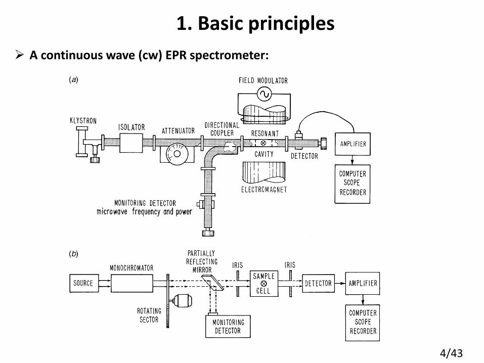
1. Basic principles

A continuous wave (cw) EPR spectrometer:

5/43

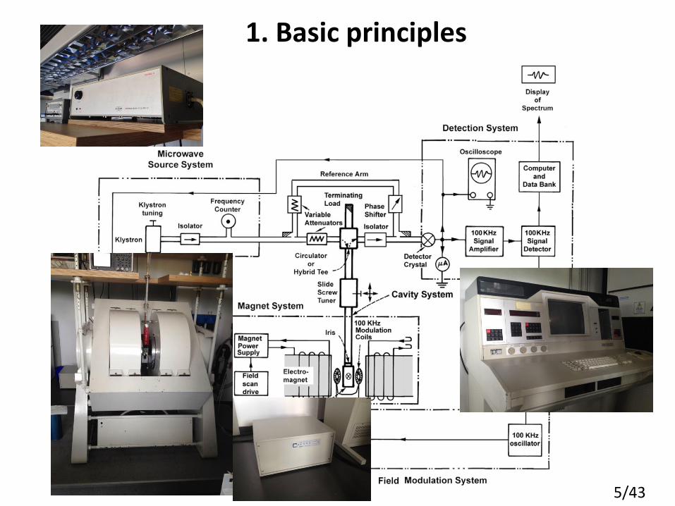
1. Basic principles

6/43

1. Basic principles

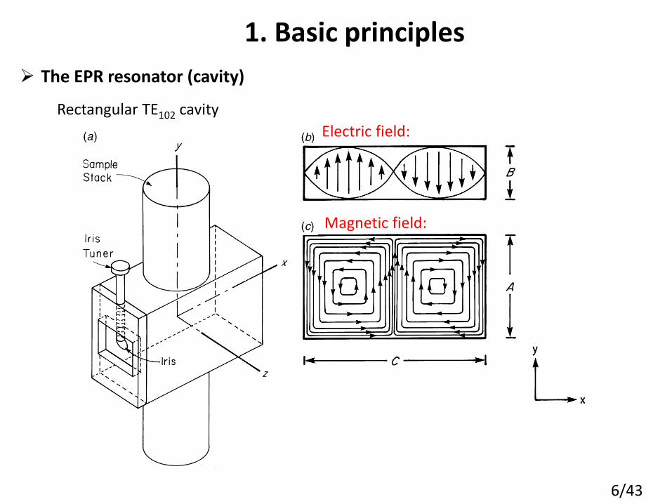
The EPR resonator (cavity)

Rectangular TE102 cavity

Electric field:

Magnetic field:

7/43

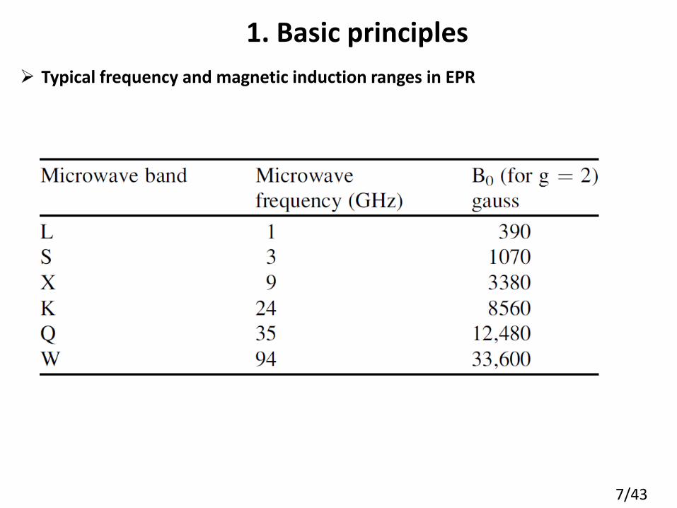
1. Basic principles

Typical frequency and magnetic induction ranges in EPR

8/43

1. Basic principles

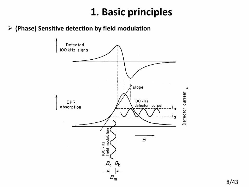
(Phase) Sensitive detection by field modulation

9/43

1. Basic principles

Samples that can be principally measured by EPR:

Free radicals in solids, liquids or in the gas phase

Transition metal ions with unpaired electron(s)

Point defects in solids

Systems with more than one unpaired electrons, e.g. triplet systems,

biradicals, multiradicals

Systems that temporarily generate states with unpaired electrons by

excitation with, e.g., light

Systems with conducting electrons

10/43

2. Electron-Nucleus Interactions

11/43

2. Electron-Nucleus Interactions

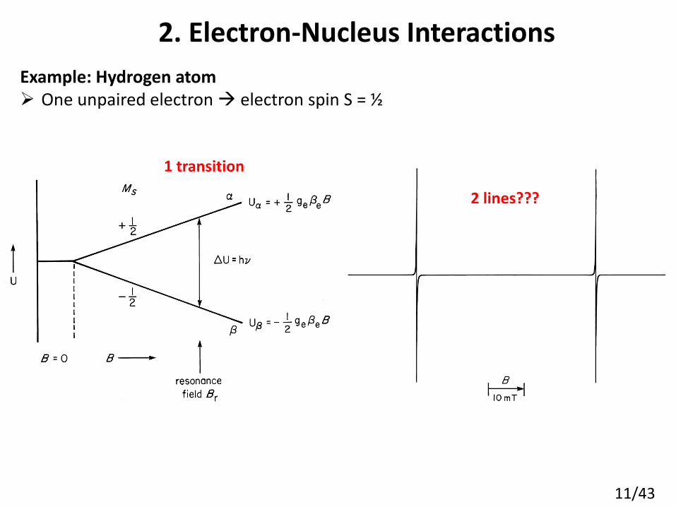
Example: Hydrogen atom One unpaired electron electron spin S = ½

2 lines???

1 transition

12/43

2. Electron-Nucleus Interactions

Example: Hydrogen atom One unpaired electron electron spin S = ½ H atom has a nuclear spin: I = ½, MI = ±½

Selection rule: DMS = ±1; DMI = 0

DMI allowed:

DMI forbidden:

Hyperfine interaction

Hyperfine interaction A0

ℎ𝜈 = 𝑔𝛽𝑒𝐵 ± 1/2A0

13/43

2. Electron-Nucleus Interactions

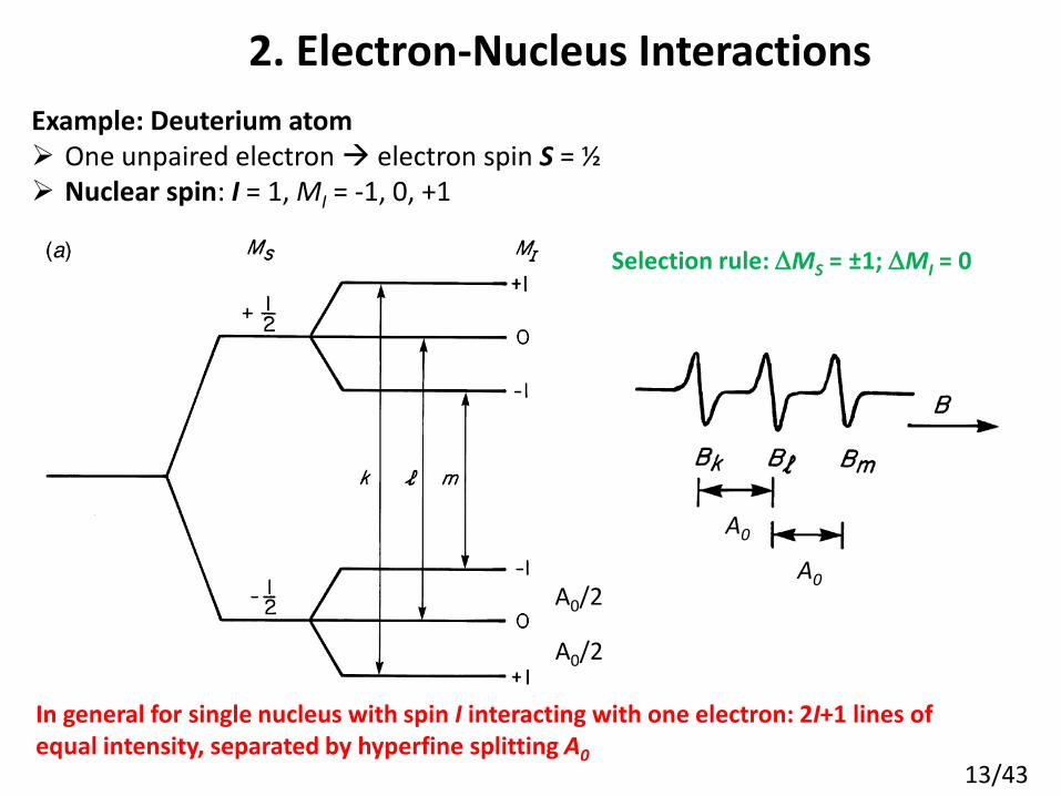
Example: Deuterium atom One unpaired electron electron spin S = ½ Nuclear spin: I = 1, MI = -1, 0, +1

Selection rule: DMS = ±1; DMI = 0

In general for single nucleus with spin I interacting with one electron: 2I+1 lines of equal intensity, separated by hyperfine splitting A0

A0

A0

A0/2

A0/2

14/43

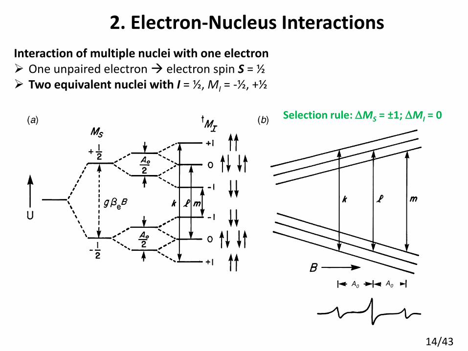
2. Electron-Nucleus Interactions

Interaction of multiple nuclei with one electron One unpaired electron electron spin S = ½ Two equivalent nuclei with I = ½, MI = -½, +½

Selection rule: DMS = ±1; DMI = 0

A0 A0

15/43

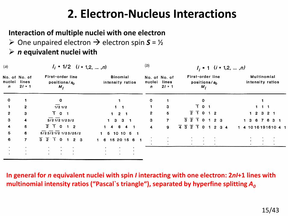
2. Electron-Nucleus Interactions

Interaction of multiple nuclei with one electron One unpaired electron electron spin S = ½ n equivalent nuclei with

In general for n equivalent nuclei with spin I interacting with one electron: 2nI+1 lines with multinomial intensity ratios (“Pascal`s triangle“), separated by hyperfine splitting A0

16/43

2. Electron-Nucleus Interactions

Interaction of multiple nuclei with one electron One unpaired electron electron spin S = ½ n equivalent nuclei with I = ½

n = 1

n = 2

n = 3

n = 4

n = 5

n = 6

n = 7

n = 8

2nI+1

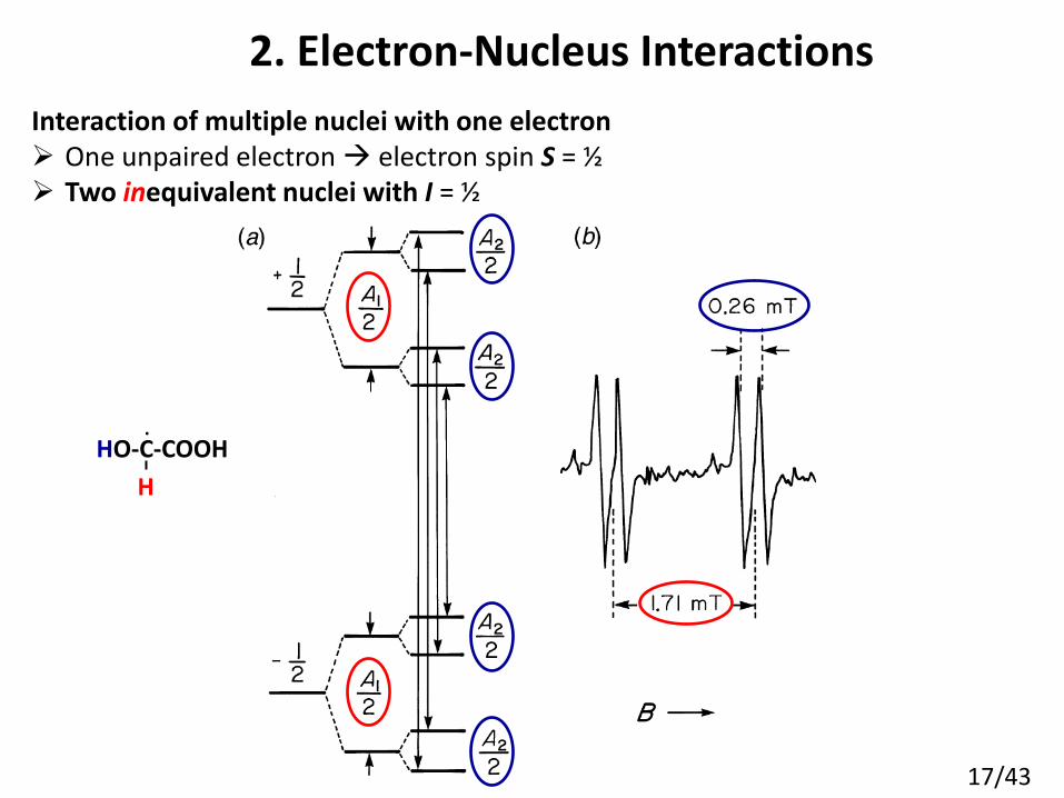
17/43

2. Electron-Nucleus Interactions

Interaction of multiple nuclei with one electron One unpaired electron electron spin S = ½ Two inequivalent nuclei with I = ½

. HO-C-COOH

H

18/43

2. Electron-Nucleus Interactions EPR spectrum of V2O5 single crystal One unpaired electron electron spin S = ½ (V4+ defect) n (?) equivalent nuclei with I = 7/2

Number of lines = 2nI+1 = 2x2x7/2+1 = 15 equally spaced lines with intensity distribution

Conclusion: electron localized at two vanadium atoms

𝑔∥ =ℎ𝜈

𝛽𝑒𝐵= 1.911

𝐴∥ = 88 G

B/G

𝐵 ∥ b

Orthorhombic space group: a=3.564(2) Å b=11.519(6) Å c=4.373(2) Å

𝐴⊥ = 33 G

𝑔⊥ = 1.983

𝐵 ∥ c

1 : 2 : 3 : 4 : 5 : 6 : 7 : 8 : 7 : 6 : 5 : 4 : 3 : 2 : 1

19/43

3. Anisotropy

20/43

3. Anisotropy

Cubic symmetry (cubal, octahedral, tetrahedral coordination)

(Uni)Axial Symmetry

Orthorhombic Symmetry

Cubic Symmetry:

Electron in environment with:

ℋ = 𝛽𝑒 𝑔𝑥𝐵𝑥𝑆 𝑥 + 𝑔𝑦𝐵𝑦𝑆 𝑦 + 𝑔𝑧𝐵𝑧𝑆 𝑧 = 𝛽𝑒[𝐵𝑥 𝐵𝑦 𝐵𝑧] ∙

𝑔𝑥 0 00 𝑔𝑦 0

0 0 𝑔𝑧

∙

𝑆 𝑥𝑆 𝑦

𝑆 𝑧

= 𝛽𝑒𝐁T ∙ 𝑔 ∙ 𝐒

Spin Hamiltonian:

𝑔𝑥 = 𝑔𝑦 = 𝑔𝑧 Isotropic g factor (independent on magnetic field direction): g is a scalar constant

F center in NaCl:

z

x y

ℋ = 𝛽𝑒𝑔(𝐵𝑥𝑆 𝑥 + 𝐵𝑦𝑆 𝑦 + 𝐵𝑧𝑆 𝑧)

Row vector

square matrix

column vector

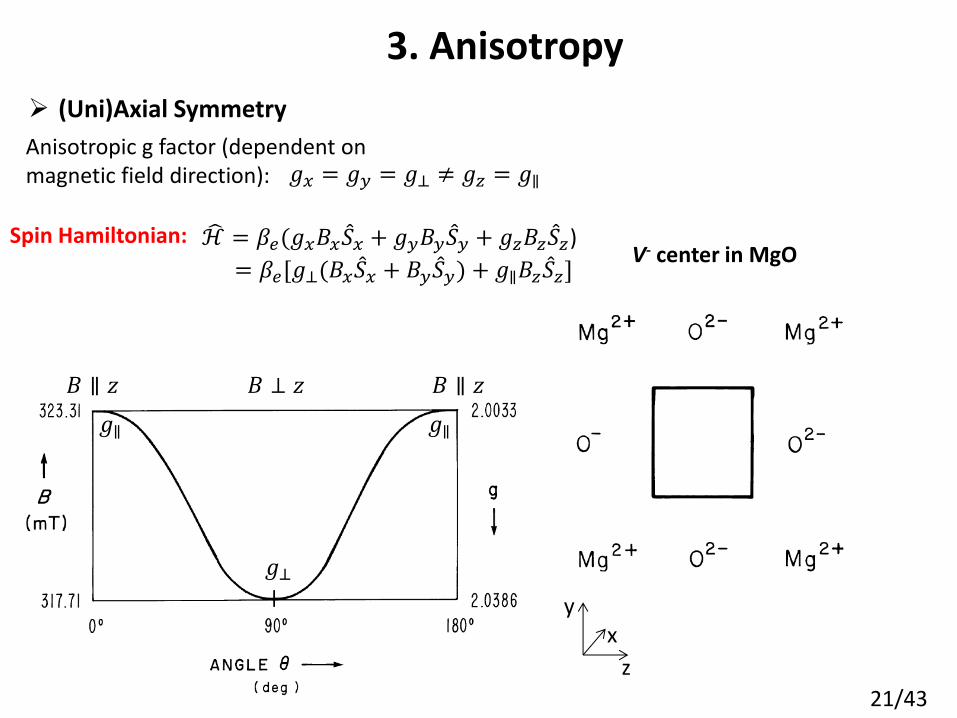
21/43

3. Anisotropy

(Uni)Axial Symmetry

ℋ = 𝛽𝑒(𝑔𝑥𝐵𝑥𝑆 𝑥 + 𝑔𝑦𝐵𝑦𝑆 𝑦 + 𝑔𝑧𝐵𝑧𝑆 𝑧)

= 𝛽𝑒[𝑔⊥(𝐵𝑥𝑆 𝑥 + 𝐵𝑦𝑆 𝑦) + 𝑔∥𝐵𝑧𝑆 𝑧]

Spin Hamiltonian:

𝑔𝑥 = 𝑔𝑦 = 𝑔⊥ ≠ 𝑔𝑧 = 𝑔∥ Anisotropic g factor (dependent on magnetic field direction):

V- center in MgO

𝑔⊥

𝑔∥ 𝑔∥

z

x y

𝐵 ∥ 𝑧 𝐵 ∥ 𝑧 𝐵 ⊥ 𝑧

22/43

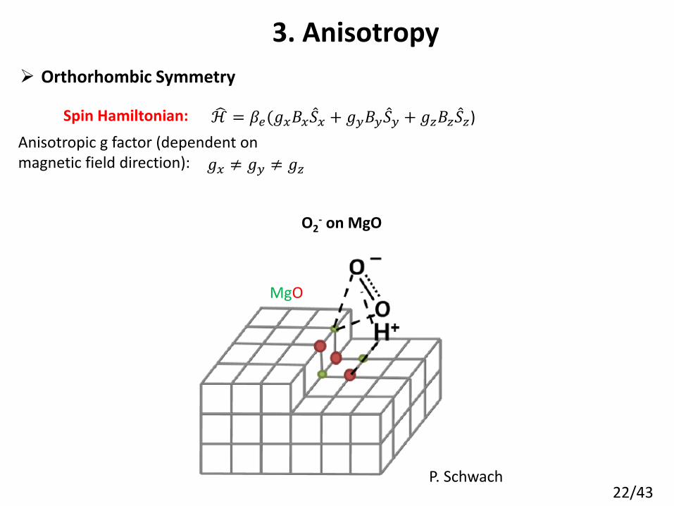
3. Anisotropy

Orthorhombic Symmetry

ℋ = 𝛽𝑒(𝑔𝑥𝐵𝑥𝑆 𝑥 + 𝑔𝑦𝐵𝑦𝑆 𝑦 + 𝑔𝑧𝐵𝑧𝑆 𝑧)

Spin Hamiltonian:

𝑔𝑥 ≠ 𝑔𝑦 ≠ 𝑔𝑧

Anisotropic g factor (dependent on magnetic field direction):

O2- on MgO

MgO

P. Schwach

23/43

3. Anisotropy

Crystalline powders: principal axis has all possible orientations relative to the direction of the magnetic field

B

V- center in MgO

24/43

3. Anisotropy Crystalline powder S = ½, I = 0 Uniaxial local symmetry

First derivative

𝜃: Angle between magnetic field and principal symmetry axis of any spin system in the sample

dA=

Fraction of symmetry axes between q and q +dq

𝑃 𝜃 d𝜃 =𝑑𝐴

𝐴𝑠𝑝ℎ𝑒𝑟𝑒~𝑃 𝐵 d𝐵

𝑃 𝜃 d𝜃 =𝑑𝐴

4𝜋𝑟2 =1

2𝑠𝑖𝑛𝜃d𝜃

Probability of a spin system experiencing a resonant field between B and B+dB

25/43

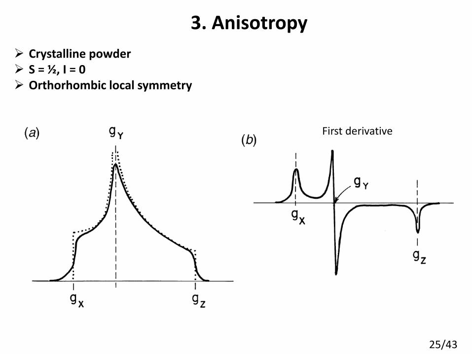
3. Anisotropy

Crystalline powder S = ½, I = 0 Orthorhombic local symmetry

First derivative

26/43

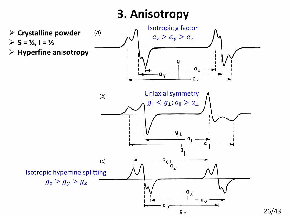
3. Anisotropy

Crystalline powder S = ½, I = ½ Hyperfine anisotropy

Isotropic g factor 𝑎𝑧 > 𝑎𝑦 > 𝑎𝑥

Uniaxial symmetry 𝑔∥ < 𝑔⊥; 𝑎∥ > 𝑎⊥

Isotropic hyperfine splitting 𝑔𝑧 > 𝑔𝑦 > 𝑔𝑥

27/43

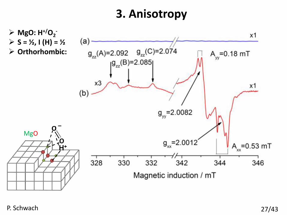
3. Anisotropy

MgO: H+/O2-

S = ½, I (H) = ½ Orthorhombic:

MgO

P. Schwach

28/43

4. Electron-Electron Interactions

29/43

4. Electron-Electron Interactions

E.g. O2, V3+, Ni2+, Fe3+

Electron exchange interaction

Singlet Triplet Triplet ground state

Stabilization by exchange interaction

Intersystem crossing

Singulet state

Triplet state

Isotropic field:

30/43

4. Electron-Electron Interactions

Electron-electron dipole interaction ℋ = 𝑔𝛽𝑒(𝐵𝑥𝑆 𝑥 + 𝐵𝑦𝑆 𝑦 + 𝐵𝑧𝑆 𝑧) Only Zeeman effect (S = ½, isotropic g factor, I = 0):

With electron-electron dipole (anisotropic) interaction (fine coupling) (S = 1, isotropic g factor, I = 0):

ℋ = 𝑔𝛽𝑒 𝐵𝑥𝑆 𝑥 + 𝐵𝑦𝑆 𝑦 + 𝐵𝑧𝑆 𝑧 + 𝐷𝑥𝑆 𝑥2

+ 𝐷𝑦𝑆 𝑦2

+ 𝐷𝑧𝑆 𝑧2

ℋ = 𝑔𝛽𝑒𝐁T ∙ 𝐒 + 𝐷(𝑆 𝑧2

−1

3𝑆 2) + 𝐸(𝑆 𝑥

2− 𝑆 𝑦

2)

e.g. E = 0

Zero-field splitting Δ𝑀𝑆 = ±1

Δ𝑀𝑆 = ±1

In cubic coordinations: D = E = 0

31/43

4. Electron-Electron Interactions

Electron-electron dipole interaction With electron-electron dipole interaction (fine coupling) (S = 1, isotropic g factor, I = 0):

ℋ = 𝑔𝛽𝑒𝐁T ∙ 𝐒 + 𝐷(𝑆 𝑧2

−1

3𝑆 2 + 𝐸(𝑆 𝑥

2− 𝑆 𝑦

2)

In cubic coordinations: D = E = 0

? For high spin systems, e.g. Fe3+: S = 5/2

Second order term ~S2

a: Fourth-order (high spin) parameter for cubic coordination

Fe3+ in cubic coordination

32/43

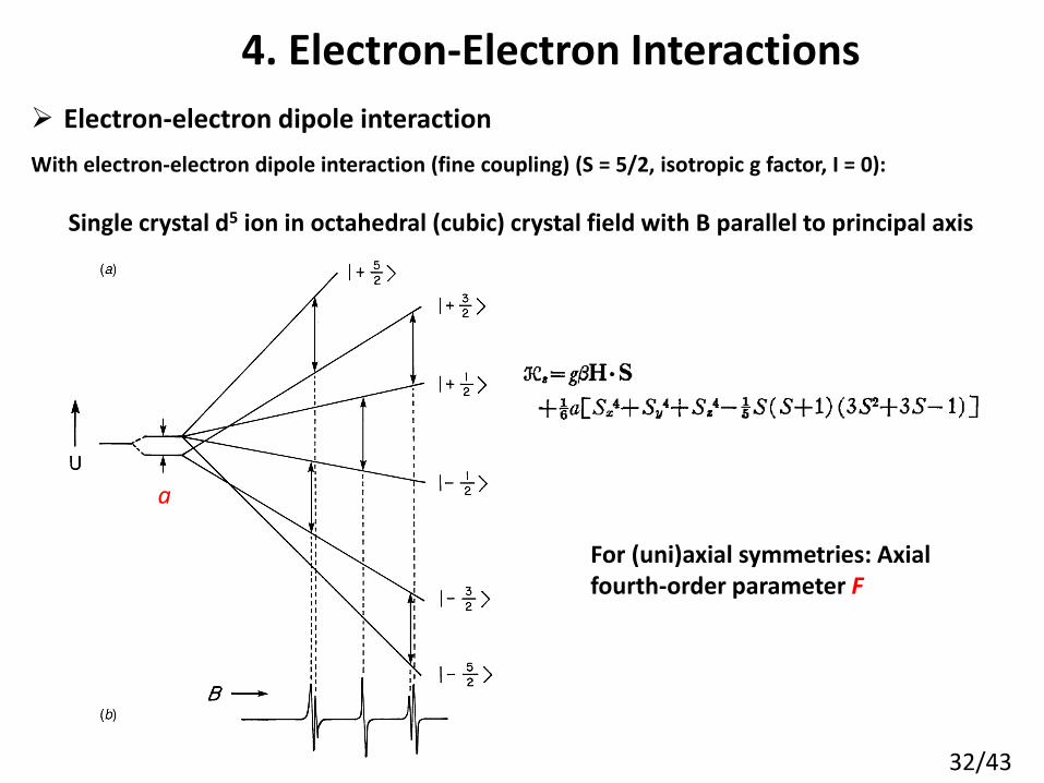
4. Electron-Electron Interactions

Electron-electron dipole interaction With electron-electron dipole interaction (fine coupling) (S = 5/2, isotropic g factor, I = 0):

a

Single crystal d5 ion in octahedral (cubic) crystal field with B parallel to principal axis

For (uni)axial symmetries: Axial fourth-order parameter F

33/43

The complete (simplified) Spin Hamiltonian

ℋ = 𝑔𝛽𝑒𝐁T ∙ 𝐒 + 𝐒 T ∙ 𝐃 ∙ 𝐒 + 𝐒 T ∙ 𝐀 ∙ 𝐈

Zeeman splitting: g tensor

Fine coupling (high spin electron-electron interactions): D, E, a, F

Nuclear hyperfine coupling (electron-nucleus interactions): A tensor

34/43

Mn Sys1.S = 5/2; Sys1.g = 2.0007; Sys1.Nucs = '55Mn'; Sys1.A = -244; Sys1.AStrain = 0; Sys1.aF = [60 0]; Sys1.lwpp = 0.1; Sys1.D = 90; Sys1.DStrain = 120; Sys1.weight = 100; Fe Sys2.S = 5/2; Sys2.g = 2.0027; % isotropic g Sys2.lwpp = [0.5 0.0]; % Gaussian, Lorentzian peak to peak width, mT Zero-field splitting in terms of D and E Sys2.D = [120 0]; %in MHz Sys2.DStrain = [600 0]; Sys2.aF=[650 0]; Sys2.aFStrain = [0 0] Sys2.weight=16000 Cr Sys3.S=3/2; Sys3.g=1.98; Sys3.Nucs='Cr'; Sys3.A=3; Sys3.lwpp=0.2; Sys3.weight=5;

Fe3+, Mn2+, Cr3+ in MgO

Spectrum Simulation with EasySpin®

35/43

5. Linewidths

36/43

5. Linewidths

Spin relaxation: spin-lattice relaxation time t1 (spin interaction with surroundings, longitudinal relaxation time)

37/43

5. Linewidths

Spin relaxation: spin-spin relaxation time t2 (spin spin interaction, transversal relaxation time) M precesses about B0 with

angular frequency 𝜔𝐿 = −𝛾𝑒𝐁0 (Larmor frequency)

𝜔𝐿

Longitudinal magnetization Mz = const.

Transversal Mx, Mz oscillate, no net transversal magnetization

Frame rotates with the angular frequency w

Superposition of a rotating perpendicular field B1

B1

y

x

Net transversal magnetization (all spins rotate in phase with w)

Mxy

y

x

Transversal magnetization decays with t2

𝜔

Mz

𝑀𝑥𝑦 = 𝑀𝑥𝑦(0)𝑒−𝑡/𝜏2

At resonance: 𝜔 = 𝜔𝐿

38/43

5. Linewidths

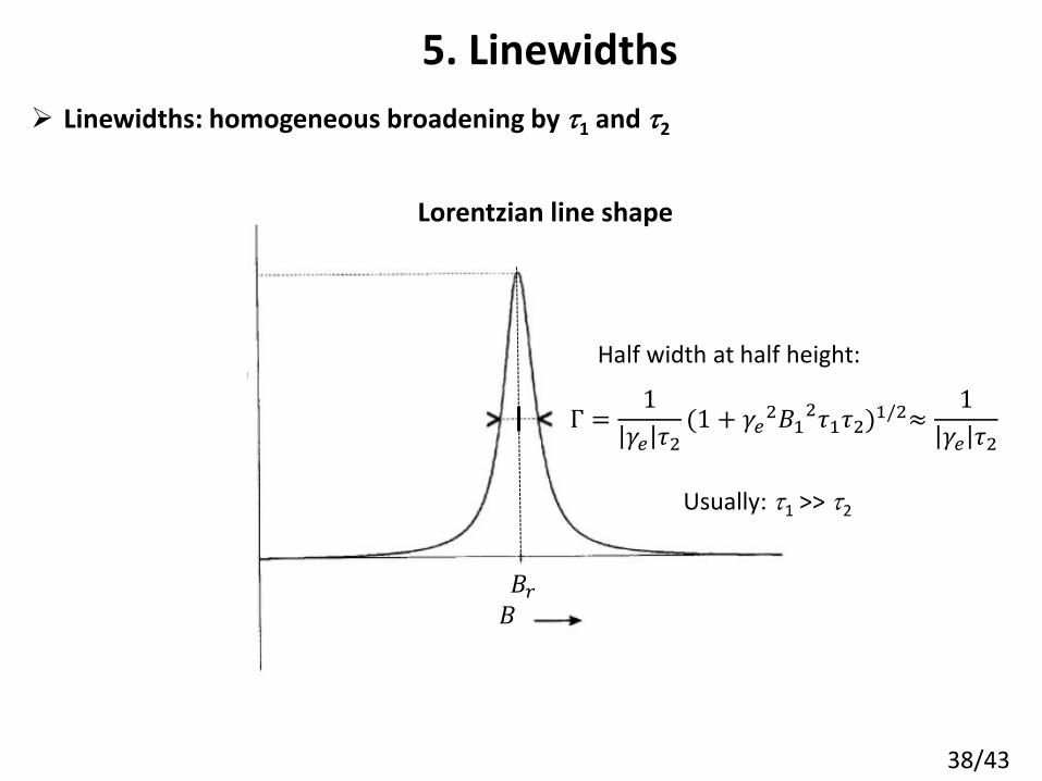
Linewidths: homogeneous broadening by t1 and t2

Lorentzian line shape

Γ =1

𝛾𝑒 𝜏2(1 + 𝛾𝑒

2𝐵12𝜏1𝜏2)1/2≈

1

𝛾𝑒 𝜏2

𝐵 𝐵𝑟

Half width at half height:

Usually: t1 >> t2

39/43

5. Linewidths

Linewidths: inhomogeneous broadening by superposition of spectra from individual equivalent spins

Gaussian(-Lorentzian) line shape

Caused by • An inhomogenous external magnetic field • Unresolved hyperfine structure • Anisotropic interactions • Dipolar interactions

B

40/43

5. Linewidths

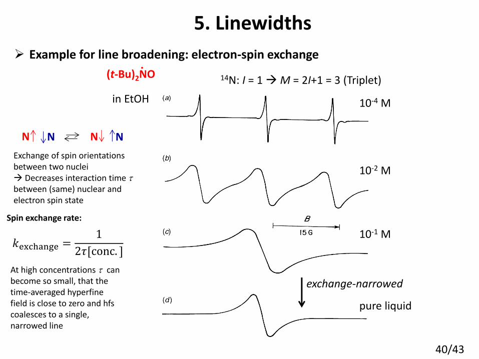
Example for line broadening: electron-spin exchange

(t-Bu)2NO .

in EtOH 10-4 M

10-2 M

10-1 M

pure liquid

14N: I = 1 M = 2I+1 = 3 (Triplet)

exchange-narrowed

N N N N

Exchange of spin orientations between two nuclei Decreases interaction time t between (same) nuclear and electron spin state

𝑘exchange =1

2𝜏[conc. ]

At high concentrations t can become so small, that the time-averaged hyperfine field is close to zero and hfs coalesces to a single, narrowed line

Spin exchange rate:

41/43

5. Linewidths

Example for line broadening: electron-spin exchange

V/SBA-15 51V: I = 7/2

Differentiation between isolated and strongly interacting V atoms possible

A. Wernbacher

42/43 A. Wernbacher

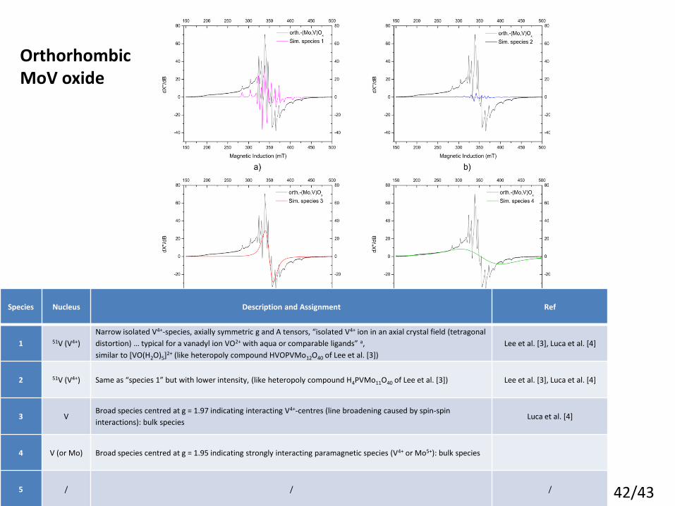
5. Linewidths Orthorhombic MoV oxide

51V: I = 7/2

Species Nucleus Description and Assignment Ref

1 51V (V4+)

Narrow isolated V4+-species, axially symmetric g and A tensors, “isolated V4+ ion in an axial crystal field (tetragonal

distortion) … typical for a vanadyl ion VO2+ with aqua or comparable ligands” a,

similar to [VO(H2O)5]2+ (like heteropoly compound HVOPVMo12O40 of Lee et al. [3])

Lee et al. [3], Luca et al. [4]

2 51V (V4+) Same as “species 1” but with lower intensity, (like heteropoly compound H4PVMo11O40 of Lee et al. [3]) Lee et al. [3], Luca et al. [4]

3 V Broad species centred at g = 1.97 indicating interacting V4+-centres (line broadening caused by spin-spin

interactions): bulk species Luca et al. [4]

4 V (or Mo) Broad species centred at g = 1.95 indicating strongly interacting paramagnetic species (V4+ or Mo5+): bulk species

5 / / /

43/43

J. A. Weil, J. R. Bolton, “Electron paramagnetic resonance“, John Wiley & Sons 2007

(comprehensive book about cw-EPR theory, also as e-book available)

G. R. Eaton, S. S. Eaton, D. P. Barr, R. T. Weber, “Quantitative EPR”; Springer 2010

A. Schweiger, “Pulsed Electron Spin Resonance Spectroscopy: Basic principles,

Techniques, and Examples of Applications“, Angew. Chem. Int. Ed. 1991, 30, 265-292

A. Schweiger, G. Jeschke, “Principles of pulse electron paramagnetic resonance“,

Oxford Univ. Press 2001

P. Rieger, “Electron Spin Resonance: Analysis and Interpretation”, Royal Soc. of

Chemistry 2007 (also as e-book available)

6. Literature