EXAM PROBLEMS IN ECON4140/4145 … PROBLEMS IN ECON4140/4145 MATHEMATICS 3 DIFFERENTIAL EQUATIONS,...

EXAM PROBLEMS

IN

ECON4140/4145 MATHEMATICS 3

DIFFERENTIAL EQUATIONS,

STATIC AND DYNAMIC OPTIMIZATION

Department of Economics, University of Oslo2008

Preface

The problems in this collection are (mostly) taken from exams in mathematics foreconomists at the Department of Economics, University of Oslo. Answers to the problemsare supplied at the back. A few minor errors in the 2004 printing have been corrected.We thank Li Cen for excellent help with this booklet.

Oslo, July 2005,

Arne Strøm and Knut Sydsæter

For this new edition we have added two sections of problems on difference equations anddynamic programming.

Oslo, April 2008,

Arne Strøm and Knut Sydsæter

Contents

1 Linear Algebra . . . . . . . . . . . . . . . . . . . . . . . . . . . . . . . . . . 12 Multivariable Calculus . . . . . . . . . . . . . . . . . . . . . . . . . . . . . . 53 Static Optimization. Kuhn–Tucker Theory . . . . . . . . . . . . . . . . . 64 Integration . . . . . . . . . . . . . . . . . . . . . . . . . . . . . . . . . . . . . 115 Differential Equations of the First Order . . . . . . . . . . . . . . . . . . . 136 Differential Equations of the Second Order . . . . . . . . . . . . . . . . . 157 Systems of Differential Equations . . . . . . . . . . . . . . . . . . . . . . . 178 Calculus of Variations . . . . . . . . . . . . . . . . . . . . . . . . . . . . . . 199 Control Theory . . . . . . . . . . . . . . . . . . . . . . . . . . . . . . . . . . 22

10 Difference equations . . . . . . . . . . . . . . . . . . . . . . . . . . . . . . . 2611 Dynamic programming . . . . . . . . . . . . . . . . . . . . . . . . . . . . . 27

Answers . . . . . . . . . . . . . . . . . . . . . . . . . . . . . . . . . . . . . . 29

4145ex3 29.4.2008 621

1. Linear Algebra

Problem 1-01

(a) Let the matrix A be defined by A =(

1 23 0

). Compute A2 and A3.

(b) Find the eigenvalues of A and corresponding eigenvectors.

(c) Let P =(

2 1−3 1

). Compute P−1, and show that A = P

(−2 00 3

)P−1.

Problem 1-02

(a) Find the eigenvalues of the matrix Aa =

⎛⎝ 2a 0 0

0 0 −a2 − a 1 2

⎞⎠, a ≤ 1

(b) Find corresponding eigenvectors in the cases (i) a = 1 and (ii) a = −3.

Problem 1-03

Given three linearly independent vectors a, b and c in Rn.

(a) Are a − b, b − c and a − c linearly independent?

(b) Let d = 4a − b − c. Is it possible to find numbers x, y and z such that

x(a − b) + y(b − c) + z(a − c) = d ?

Problem 1-04

Let A be the matrix A =(

1 22 1

).

(a) Find the eigenvalues and a set of corresponding eigenvectors of A.

(b) Let x0, x1, x2, . . . be a sequence of vectors given by

x0 =(

12

)and xt+1 = Axt for t = 0, 1, 2, . . .

Show that x0 can be written as a linear combination of eigenvectors of A. Use thisto find xt for t = 1, 2, 3, . . .

Problem 1-05

Determine the eigenvalues of the matrix

Aa =

⎛⎝ 2a 0 0

0 0 −a2 − a 1 2

⎞⎠ , a ≤ 1

Find also the corresponding eigenvectors when a = 1 and when a = −3.

14145ex3 29.4.2008 621

Problem 1-06

(a) Find the rank of Dt =

⎛⎜⎝

t 0 0 10 2 t 31 −2 t 02t 1 0 3

⎞⎟⎠ for all values of t.

(b) Let A, B and C be n×n matrices where A and C are invertible. Solve the followingmatrix equation for X:

CB + CXA−1 = A−1

Problem 1-07

(a) Let A =

⎛⎝ a 0 0

0 b 00 0 c

⎞⎠ where a, b, and c are different from 0. Find A−1.

(b) Given a 3×3 matrix B whose column vectors b1, b2 and b3 are mutually orthogonaland different from the zero vector. Put A = B′B and show that A is a diagonalmatrix.

(c) Find B−1 expressed in terms of A = B′B and B.

(d) Prove that the columns of P =

⎛⎝ 1 −8 4

−8 1 44 4 7

⎞⎠ are mutually orthogonal. Find P−1

by using the results above.

Problem 1-08

Consider the matrix A =

⎛⎝ 3 −1 1

−1 3 11 1 3

⎞⎠.

(a) Show that the characteristic polynomial of A can be written in the form(4 − λ)(λ2 + aλ + b) for suitable constants a and b. Find the eigenvalues of A.

(b) Show that

⎛⎝ 1/

√2

01/

√2

⎞⎠,

⎛⎝ 1/

√6

−2/√

6−1/

√6

⎞⎠, and

⎛⎝ 1/

√3

1/√

3−1/

√3

⎞⎠ are eigenvectors of A.

Let C be the matrix with the three vectors from part (b) as columns.

(c) Show that CC′ = I3 (the identity matrix of order 3), and use this to find the inverseof C. Compute C−1AC. (This will be a diagonal matrix.)

(d) Let D = diag(d1, d2, d3) be a diagonal matrix, and let B = CDC−1. Show that

B2 = CD2C−1, and that B2 = A for suitable values of d1, d2 and d3.

Problem 1-09

(a) Find the rank of

⎛⎜⎝

1 2 0 31 1 2 00 −1 2 −31 0 −2 0

⎞⎟⎠.

(b) For what values of x, y and z are the three vectors (x, 1, 0, 1), (2, y,−1, 0) and(0, 2, 2x, z) linearly independent?

24145ex3 29.4.2008 621

Problem 1-10

Let the matrices Ak and P be given by

Ak =

⎛⎝ 1 k 0

3 −2 −10 −1 1

⎞⎠ and P =

⎛⎝ 1/

√10 −3/

√35 3/

√14

0 5/√

35 2/√

143/

√10 1/

√35 −1/

√14

⎞⎠

(a) Determine the rank of Ak for all values of k.(b) Find the characteristic equation of Ak and determine the values of k that make all

the eigenvalues real.(c) Show that the columns of P are eigenvectors of A3, and compute the matrix product

P′A3P.

Problem 1-11

(a) Consider the equation system

a11x1 + a12x2 + · · · + a15x5 = c1

a21x1 + a22x2 + · · · + a25x5 = c2

a31x1 + a32x2 + · · · + a35x5 = c3

(∗)

where the coefficient matrix has rank 3 and x1, . . . , x5 are the unknowns. Does (∗)always have a solution? And if so, how many degrees of freedom are there?

(b) Add the equation a41x1 + · · · + a45x5 + a46x6 = c4 to system (∗), where x6 is anadditional unknown. Describe possible solutions, including the degrees of freedom,in the new system. (Explicit solutions are not required.)

Problem 1-12

(a) Consider the matrix D(s) =

⎛⎜⎝

1 2s 1 1−2 1 −2 3s

1 1 − s −1 5−1 2 s −3

⎞⎟⎠. Find a necessary and suf-

ficient condition for D(s) to have rank 4. What is the rank if s = 1?(b) Determine the number of degrees of freedom for the equation system

x + 2y + z + w = 0−2x + y − 2z + 3w = 0

x − z + 5w = 0−x + 2y + z − 3w = 0

Problem 1-13

(a) Let A be a symmetric n × n matrix with |A| �= 0, let B be a 1 × n matrix, and letX be an n × 1 matrix. Consider the expression

(X + 12A

−1B′)′A(X + 12A

−1B′) − 14BA−1B′ (∗)

Expand and simplify.(b) Suppose that A is symmetric and positive definite (i.e. Y′AY > 0 for all n × 1

matrices Y �= 0). Using (∗), find the matrix X that minimizes the expressionX′AX + BX.

34145ex3 29.4.2008 621

Problem 1-14

Given the matrix A =(

1 1 11 2 3

).

(a) Find the rank of A, show that (AA′)−1 exists, and find this inverse.

(b) Compute the matrix C = A′(AA′)−1, and show that ACb = b for every 2 × 1matrix (2-dimensional column vector) b.

(c) Use the results above to find a solution of the system of equations

x1 + x2 + x3 = 1x1 + 2x2 + 3x3 = 1

(d) Consider in general a linear system of equations

Ax = b, where A is an m × n matrix, m ≤ n (∗)

It can be shown that if r(A) = m, then r(AA′) = m. Why does this imply that(AA′)−1 exists? Put C = A′(AA′)−1, and show that if v is an arbitrary m × 1vector, then ACv = v. Use this to show that x = Cb must be a solution of (∗).

Problem 1-15

Define the matrix Aa for all real numbers a by Aa =

⎛⎝ a 0 1

a a 11 1 1

⎞⎠.

(a) Compute the rank of Aa for all values of a.

(b) Find all eigenvalues and eigenvectors of A0. (NB! Here a = 0.) Show that eigenvec-tors corresponding to different eigenvalues are mutually orthogonal.

(c) Discuss the rank of the matrix product AaAb for all values of a and b.

Problem 1-16

Let A =

⎛⎜⎝

4 1 1 11 4 1 11 1 4 11 1 1 4

⎞⎟⎠.

(a) Compute the eigenvalues of A. (Hint: You can use (without proof) the formula

∣∣∣∣∣∣∣∣a + b a . . . a

a a + b . . . a...

.... . .

...a a . . . a + b

∣∣∣∣∣∣∣∣= bn−1(na + b)

where n is the order of the determinant.)

(b) One of the eigenvalues has multiplicity 3. Find three linearly independent eigenvec-tors associated with this eigenvalue. Find also an eigenvector associated with thefourth eigenvalue.

44145ex3 29.4.2008 621

Problem 1-17

Given the matrices A =

⎛⎝ a b b

b a bb b a

⎞⎠ and E =

⎛⎝ 1 1 1

1 1 11 1 1

⎞⎠.

(a) Find the eigenvalues and eigenvectors of E.(b) Find numbers p and q such that A = pI3 + qE.(c) Show that if x0 is an eigenvector of E, then x0 is also an eigenvector of A.(d) Find the eigenvalues of A.

Problem 1-18

Given the matrix A =

⎛⎝−2 −1 4

2 1 −2−1 −1 3

⎞⎠.

(a) Show that x1 =

⎛⎝ 1

01

⎞⎠, x2 =

⎛⎝ 1

−10

⎞⎠, and x3 =

⎛⎝ 1

11

⎞⎠ are eigenvectors of A, and

find the corresponding eigenvalues.(b) Let B = AA. Show that Bx2 = x2 and Bx3 = x3. Is Bx1 = x1?(c) Let C be an arbitrary n × n matrix such that C3 = C2 + C. Show that if λ is an

eigenvalue of C, then λ3 = λ2 + λ. Show that C + In has an inverse.

Problem 1-19

(a) Find the eigenvalues of the matrix A =

⎛⎝−a2b 0 ab

0 c 0−ab 0 b

⎞⎠.

(b) Let H be a 3× 3 matrix with eigenvalues λ1, λ2 and λ3, and let α be a number �= 0.Show that αλ1, αλ2 and αλ3 are eigenvalues of the matrix K = αH.

(c) Find the eigenvalues of B =1

1 − a2

⎛⎝−4a2 0 4a

0 1 − a2 0−4a 0 4

⎞⎠, a �= ±1.

(d) Find a matrix P such that P−1BP =

⎛⎝ 0 0 0

0 1 00 0 4

⎞⎠ = D, where B is the matrix in

(c). Find then a matrix C such that C2 = B. (Hint: Find first a diagonal matrixE such that E2 = D. Make use of the formula PE2P−1 = PEP−1PEP−1 to findC expressed in terms of E and P.)

2. Multivariable Calculus

Problem 2-01

Decide if the following functions are (strictly) concave/convex, quasiconcave/quasiconvexin their domains. (In (a) and (c) you should not differentiate.)(a) (i) f(x, y) = 10x0.5y0.3, x ≥ 0, y ≥ 0 (ii) g(x, y) = 10x1/3y5/3, x ≥ 0, y ≥ 0(b) F (x1, x2, x3) = 3 − x2

1 − x1x2 − 2x22 + x1x3 − 5x2

3

(c) G(x, y) =√

ln(x + y − 4). (Where is G defined?)(d) H(x1, x2, x3) = 3x2

1 − 2x1x2 − 4x1x3 + x22 + 2x2

3

54145ex3 29.4.2008 621

Problem 2-02

For which values of the constants a and b is f(x, y) = eax+by2defined for all x and y

concave/convex?

Problem 2-03

Let f be defined for all x and y by f(x, y) = 2x − y − ex − ex+2y. Is f concave/convex?

Problem 2-04

Prove that f(x, y) = e−x√

1 + y2 is strictly convex for |y| < 1.

Problem 2-05

Define the function f for all x, y by f(x, y) = 3 sin 2x + 3y − 3y2 + 8. Show that f isconcave in the rectangle R =

{(x, y) : 0 < x < π/2, 0 < y < 1

}.

Problem 2-06

Let D be the set of points (x, y) with −1 < x < 1 and −1 < y < 1, and let

f(x, y) =112

(x − y)4 − (x − y)2 − (x + y)2

(a) Show that f is neither convex nor concave in D.(b) Find the subset of D at which f is concave.

Problem 2-07

Let f(x, y) = (lnx)a(ln y)b, defined for x > 1, y > 1. Assume that a > 0, b > 0 anda + b < 1. Compute the Hessian matrix H of f and show that f is strictly concave.

3. Static Optimization. Kuhn-Tucker Theory

Problem 3-01

Solve the problem maxx1/2y1/3 subject to 3x + 4y ≤ 25.

Problem 3-02

Consider the problem

max f(x, y) = x2 + y2 subject to g(x, y) = 5x2 + 6xy + 5y2 ≤ 1

(a) Write out the necessary Kuhn–Tucker conditions for a point (x, y) to solve theproblem, and find all points that satisfy the conditions. Do any of those pointssolve the problem?

(b) The admissible set is the set of points inside an ellipse in the xy-plane. Explain whythe problem can be interpreted as that of finding the point or points on the ellipseg(x, y) = 1 with the greatest distance from the origin.

(c) Determine the approximate changes in the maximum value of f(x, y) if the constraintg(x, y) ≤ 1 is replaced by g(x, y) ≤ 1.1.

64145ex3 29.4.2008 621

Problem 3-03

(a) Write down the Kuhn–Tucker conditions for the problem

max x + xy subject to y + x2ey ≤ 1

(b) Prove that (0,−1) and (1, 0) both satisfy the conditions and find the associatedLagrange multipliers.

Problem 3-04

Solve the following problem:

minimize f(x, y) = ex+y + ey + 2x + y s.t. x ≥ −1, y ≥ −1, x + y ≥ 0

Problem 3-05


maximize x2ye−x−y s.t. x ≥ 1, y ≥ 1, x + y ≥ 4

(a) Write down the Kuhn–Tucker conditions for the problem.

(b) Find all the solutions to these conditions.

(c) (Optional.) Have you in (b) found the solution to the problem?

Problem 3-06

(a) Solve the nonlinear programming problem

maximize f(x, y, z) = x + ln(1 + z) subject to

{x2 + y2 ≤ 1

x + y + z ≤ 1

(b) What is the approximate change in the optimal value of f(x, y, z) if the secondconstraint is replaced by x + y + z ≤ 1.02 ?

Problem 3-07


(∗) max (2x + y) s.t.

{(x + 1)2 + y2 ≤ 4

x2 + (y + 1)2 ≤ 4x ≥ 0, y ≥ 0

(a) Let S be the set of all (x, y) which satisfy all the four constrains. Sketch S in thexy-plane, and draw some level curves for f(x, y) = 2x + y.

(b) Solve problem (∗) by a geometric argument.

(c) Write down the Kuhn–Tucker conditions. Verify that the point (x0, y0) you foundin (b) satisfies the Kuhn–Tucker conditions.

(d) Suppose that x2 + (y + 1)2 ≤ 4 in (∗) is replaced by x2 + (y + 1)2 ≤ 4.1. Estimatethe approximate change in the maximum value of 2x + y.

74145ex3 29.4.2008 621

Problem 3-08

Solve the problem

max[ln(x2 + 2y) − 1

2x2 − y

]subject to y ≥ 2/x, x ≥ 1, y ≥ 1

Problem 3-09

Consider the nonlinear programming problem

maximize x5 − y3 subject to x ≤ 1, x ≤ y

(a) Find the only possible solution to this problem.(b) Solve the problem by using iterated optimization: Find first the maximum value

f(x) in the problem to maximize x5 − y3 s.t. x ≤ y, where x is given and y varies.Then maximize f(x) subject to x ≤ 1.

Problem 3-10

Let f be a function of two variables given by

f(x, y) = −x4 − cx2 + 6xy − 6y2

where c is a constant.(a) For which values of c will f be concave in the whole plane?

Consider next the problem:

(∗) max (−x4 − y4 − 4x2 + 6xy − 6y2 + ax + by) s.t. x + y2 ≤ 1 and y ≥ −1.

Here are a and b constants.(b) Write down the Kuhn–Tucker conditions for a point (x, y) to solve (∗).(c) Find necessary and sufficient conditions on a and b for the maximum point in (∗) to

be (x, y) = (0,−1).

Problem 3-11

Let f and g be functions of two variables given by

f(x, y) = ax + by − 6x2 − 5xy − 5y2, g(x, y) = 3 − (x2 + y2)2

where a and b are constants.(a) Show that f and g are both concave in the whole plane.

Next we study the problem:

(∗) max(f(x, y) + g(x, y)

)s.t. x ≥ 1 and y ≤ √

x

(b) Write down the Kuhn–Tucker conditions for a point (x, y) to solve (∗).(c) Find necessary and sufficient conditions on a and b for the maximum point in (∗) to

be (x, y) = (1, 0).(d) Let a = 300. For which value of b will (∗) have the solution (x, y) = (4, 2)?

84145ex3 29.4.2008 621

Problem 3-12

(a) Solve the nonlinear programming problem

maximize −(

x +12

)2

− 12y2 subject to

{y ≥ e−x

y ≤ 2/3

(Hint: You may need the fact that the equations e−2x = 2x+1 and y2 = e1−y2have

the solutions x = 0 and y = ±1, respectively.)

(b) Can you give a geometric interpretation of the problem?

Problem 3-13


(∗)maximize a ln(z + 1) − z − 2x − y

s.t. x ≥ 0, y ≥ 0, z ≥ 0 and z2 ≤ x + y

where a is a positive constant.

(a) Write down the Kuhn-Tucker conditions for the solution of (∗).

(b) Find the solutions of the Kuhn-Tucker conditions. Consider the cases a > 1 anda ≤ 1 separately.

(c) Prove that the points you found in (b) really solve problem (∗).

Problem 3-14

(a) Solve the problem minimize [(x − 2)2 + (y − 2)2] s.t.

{x + y ≤ 2,

x2 − 4x + y ≤ −2.

(b) Can you give a geometric interpretation of the problem and thereby confirm theanswer in (a)?

Problem 3-15


(P) maximize 4x + y s.t.

⎧⎪⎨⎪⎩

y − (x − 1)2 ≤ 1

y − (x − 2)2 ≤ −1x ≥ −2, y ≥ 0, x ≤ 2

(a) Sketch the admissible region, and draw some level curves for the criterion function.

(b) Make use of the figure from (a) to show that (1, 0) solves problem (P).

(c) Write down the necessary Kuhn–Tucker-conditions for the solution of (P), and showthat (1, 0) satisfies these conditions.

94145ex3 29.4.2008 621

Problem 3-16

Solve the problem

maximize (2x − x2 + 2y − y2 + z) s.t.

⎧⎪⎨⎪⎩

1 − xy ≤ 0x + y + z ≤ 4

x ≥ 0, y ≥ 0, z ≥ 0

Prove that you have really found the maximum.

Problem 3-17

Maximize ln(x + y + 3) subject to x2 + y2 + z2 ≤ 1, x + y + z ≤ 1.

Problem 3-18

Solve the problem

minimize (x + y)2 s.t. y ≥ (x − 2)2, xy ≥ 1

(Hint: Use the fact that x = 1 is a solution of the equation x(x − 2)2 = 1.)

Problem 3-19

Find the maximum of xy + ex+z subject to 0 ≤ x + z ≤ 1 − x2 − 2y2.

Problem 3-20


maximize x + y − 1 s.t.

⎧⎨⎩

x + y + z2 ≤ a

3x2 + 2y +13z ≤ 0

Here a is a constant.(a) Write down the Kuhn–Tucker conditions for a point (x, y, z) to solve the problem.

Show that if (x, y, z) solves the problem, then z ≤ 0.(b) Solve the problem when a = 0.(c) Solve the problem when a = 1.

Problem 3-21


maximize f(x, y) = (x − c)α(y − d)1−α subject to

⎧⎪⎪⎪⎨⎪⎪⎪⎩

(1) x ≥ c

(2) y ≥ d

(3) x + y ≤ 2(4) x ≤ c + d

(∗)

Here α, c, and d are constants with α ∈ (0, 1), c ≥ 0, d ≥ 0 and 2d < 2 − c.(a) Sketch the set S consisting of all (x, y) that satisfy (1)–(4). Explain why (1) and (2)

cannot be binding at the optimum.

104145ex3 29.4.2008 621

(b) Show that the problem is equivalent to

maximize[α ln(x − c) + (1 − α) ln(y − d)

]subject to

{(3) x + y ≤ 2(4) x ≤ c + d

(∗∗)

(c) Write down the Kuhn–Tucker-conditions for the solution to (∗∗) and show that (3)must be binding at the optimum. Solve the problem.

Problem 3-22


max (4z − x2 − y2 − z2) s.t.

{z ≤ xy

x2 + y2 + z2 ≤ 3

(a) Write down the Kuhn–Tucker conditions for the problem.(b) Verify that the problem has a solution, and find the solution.(c) What is the approximate change in the maximum value of 4z − x2 − y2 − z2, if the

first constraint is changed to z ≤ xy + 0.1?

Problem 3-23

(a) Find the maximum of xyz subject to

⎧⎪⎨⎪⎩

x + y + z ≤ 5xy + xz + yz ≤ 8

x ≥ 0, y ≥ 0, z ≥ 0

(b) Prove that the problem in part (a) does not have a solution if we drop the nonneg-ativity conditions on x, y, and z.

4. Integration

Problem 4-01

Define the function F for all T ≥ 0 by F (T ) =∫ T

0 f(t)e−r(t−T ) dt, where f is agiven function and r is a given number. Find an expression for F ′(T ) and show thatF ′(T ) − rF (T ) = f(T ).

Problem 4-02

Define the function F for all x > 0 by F (x) =∫ x

0ext2 dt.

(a) Find expressions for F ′(x) and F ′′(x) by using Leibniz’s formula.(b) Show that F is strictly convex on (0,∞).

Problem 4-03

Define the function g by g(x) =∫ 2π

π

sin(xt)t

dt for all x. Show that g′(1) = 0.

114145ex3 29.4.2008 621

Problem 4-04

Let y(t) be defined by y(t) =∫ t

0sin2(t + x) dx. By differentiating y(t) twice, show that

y(t) = 6 sin 2t cos 2t + 2t − 4y(t).

Problem 4-05 Compute the integral∫ 1

0

(∫ 1

0xeydy

)dx.


0

(∫ 4

0(√

xy + 2x + y) dy)dx.


0

(∫ 1

0(x√

x2 + y dx)dy.

Problem 4-08

Compute the integral∫ 1

0

(∫ π/2

0xy2 cos(x2y) dy

)dx.

Problem 4-09

Compute the double integral∫ 2π

π

∫ π

0

x

y3 cos(x2

y

)dx dy.

Problem 4-10

Let V (t) =∫ t

1

(∫ t

1 F (t, x, y) dx)dy. Use Leibniz’s formula to find an expression for V ′(t).

Problem 4-11

In a model by T. Haavelmo the following equations appear∫ t

t1

z(τ) dτ =∫ t+T (t)

t1+T (t1)x(τ) dτ for all t ≥ t1 (∗)

∫ t+T (t)

t

y(τ) dτ = 1 for all t ≥ t1 (∗∗)

In both cases find an expression for dT/dt, assuming that z(τ), x(τ), T (t), and y(τ) arewell-behaved and t1 is a constant.

124145ex3 29.4.2008 621

5. Differential Equations of the First Order

Problem 5-01

Solve the differential equations

(a) x + 4x = 3et, x(0) = 1 (b) x =e−3x

3 +√

t + 8, x(1) = 0

Problem 5-02

Solve the differential equation x =3√

ax + b

xt2, where the constant a is �= 0.

Problem 5-03

Find the solution of the following differential equation that satisfies the given initialcondition:

x = t(x − 1)2, x(0) = 3

Problem 5-04

(a) Solve the differential equation x + 4x = 4e−2t, x(0) = 1.(b) Suppose that y = (a+αk)

√t + 1 denotes production as a function of capital k, where

the factor√

t + 1 is due to technical progress. Suppose that a constant fractions ∈ (0, 1) is saved, and that capital accumulation is equal to savings, so that wehave the separable differential equation

k = s(a + αk)√

t + 1, k(0) = k0

The constants a, α and k0 are positive. Find the solution.

Problem 5-05

(a) Find the general solution of the differential equation x + 2x = 2.

(b) Find a function w = w(t) such that

w + 2w = 2, w(0) = 0 and w(−1

2)

=12

− e.

Problem 5-06

In a growth model production Q is a function of capital K and labour L. Suppose that

(i) K = γQ (investment is proportional to production)(ii) Q = KαL

(iii) L = β (the rate of change of L with respect to t is constant)Here γ, α, and β are positive constants, α < 1.(a) Derive a differential equation to determine K.(b) Solve this equation when K(0) = K0 and L(0) = L0.

134145ex3 29.4.2008 621

Problem 5-07

Find the solution of the differential equation x + 3x = t2.

Problem 5-08

Determine the solution of the differential equation

xdx

dt= −1

2(x2 − 25), x > 5 (∗)

that passes through the point P = (0, 10). What is the slope of the solution curve at P?Show that every solution of (∗) is decreasing.

Problem 5-09

Find the solution of the differential equation 3x2x = (x3+9)3/2 ln t whose solution curvepasses through the point (t, x) = (1, 3).

Problem 5-10

Find the solution of the differential equation

x = (2x + 1)4 · t3 · sin(t2)

whose integral curve passes through (t, x) = (0, 0).

Problem 5-11


e2tx + e2t(2 − 2t)x =et2+t

√1 + et

whose integral curve passes through (t0, x0) = (0, 3).

Problem 5-12


x + 3t2x = tet2−t3

whose integral curve passes through (t0, x0) = (−1, 0).

Problem 5-13

(a) Find the general solution of the differential equation x =2

t + 1x.

(b) Consider the differential equation

(t + 1)x − 2(t + 1) = 2x + (t + 1)5 (∗)

Introduce a new variable u = u(t) by putting x = (t + 1)2u, and transform equation(∗) into a simple differential equation in the unknown function u = u(t). Use thisto find the general solution of (∗).

144145ex3 29.4.2008 621

Problem 5-14

Find the general solution of the differential equation x = x3+3x2−2. (Hint: Put x = y+aand find a differential equation for y. Choose an a such that this equation becomes aBernoulli equation.)

6. Differential Equations of the Second Order

Problem 6-01

Find the general solutions of the following differential equations:

(a) x − 8x + 17 = 0 (b) x + 2x + 5x = 0

Problem 6-02

Find the general solutions of the differential equations

(a) x +72x − 2x = 0 (b) x +

72x − 2x = t + sin t

(Hint: (b) has a particular solution of the form u∗ = At + B + C sin t + D cos t.)

Problem 6-03

Find the general solutions of the following differential equations:

(i) 4x − 15x + 14x = 0 (ii) 4x − 15x + 14x = t + sin t

Problem 6-04

Find the general solution of x − 6x + 25x = t.

Problem 6-05

Find the general solution of the differential equation 3x+10x+3x = f(t) in the followingthree cases:

(i) f(t) = 0, (ii) f(t) = 8e−t + 6, (iii) f(t) = −8e−3t.

Problem 6-06

Find the general solution of the differential equation x + x + 2x = t2 + 2.

Problem 6-07

Solve the differential equations

x − ax + (a − 2)x = 0 (i)x − ax + (a − 2)x = t (a �= 2) (ii)

154145ex3 29.4.2008 621

Problem 6-08

In connection with a problem in utility theory the following differential equations areencountered:

(i) g′′(t) = −14

g′(t) (ii) g′′(t) = − 2t + 1

g′(t)

Find the general solutions of these equations.

Problem 6-09

In an economic model one encounters the differential equation

Y + (αl + β)Y + αβ(l + m)Y = −αβt − αl + β

l + m(∗)

where α, β, l and m are positive constants.

(a) Find a particular solution of (∗).

(b) Put α = 1/4, β = 3/4, l = 1 and m = 17/3, and find the general solution to theequation in this case.

(c) Discuss conditions that ensure that the solutions of (∗) give oscillations. What canyou then say about the behaviour of the solutions as t approaches infinity?

Problem 6-10

A model describing the market behaviour of firms includes the differential equation

12σ2x2V ′′(x) + μxV ′(x) − ρV (x) = w − x (x > 0) (∗)

Here σ, μ, ρ, and w are positive constants, ρ �= μ, while V (x) is an unknown function.

(a) Show that the homogeneous equation corresponding to (∗) has solutions of the formV (x) = xa. Find the general solution of the homogeneous equation.

(b) Find a particular solution of (∗).

(c) Find the general solution of the equation x2V ′′(x) + xV ′(x) − 4V (x) = 10 − x.

Problem 6-11

Consider the differential equation

x − 2(k − 1)x + (k2 − 4)x = 2e(4−k)t (∗)

where k is a real number.

(a) Find the general solution of the homogeneous equation corresponding to (∗) for allvalues of k.

(b) Find a particular solution of (∗) for each value of k.

(c) Let k = 3. Find the integral curve for (∗) that passes through the origin and is tan-gent to the t-axis at that point. Is t = 0 a local extreme point for the correspondingfunction?

164145ex3 29.4.2008 621

Problem 6-12

In an economic problem the price function p = p(t) satisfies the equation

p(t) = β

∫ t

−∞

[D(p(τ)) − S(p(τ))

]e−α(t−τ) dτ

where D(p) = a − bp is a demand function, S(p) = −c + dp is a supply function, and α,β, a, b, c, and d are positive constants.

(a) Show that p satisfies the differential equation

p + αp + β(b + d)p = β(a + c) (1)

(b) Determine the equilibrium value p∗ for (1), and find the general solution of (1).

(c) Show that (1) is stable. Decide for what values of the parameters the solutionexhibits damped oscillations about p∗.

Problem 6-13

Given the second-order differential equation

t2x + tx − x = 0, t > 0 (∗)

(a) Introduce the substitution z = tx and derive a second-order differential equationfor z. Solve this equation and find the general solution of (∗).

(b) Find the solution of (∗) with x(1) = 1 and x(1) = 1.

Problem 6-14

Solve the differential equation x + 10x + 25x = 5ekt + sin t for all values of k.

Problem 6-15

(a) Find the general solution of the differential equation 2x + 8x + 26x = e2t.

(b) Explain how to find the general solution if e2t is replaced by sin 3t.

7. Systems of Differential Equations

Problem 7-01

Given the following system of differential equations:

x = x + y + t

y = −x + 2y

Deduce a second-order differential equation for x. Solve this equation and then find thegeneral solution (x(t), y(t)) of the system.

174145ex3 29.4.2008 621

Problem 7-02

Consider the differential equation system

x = ax + 2y + α

y = 2x + ay + β(∗)

where a, α and β are constants.(a) Find the general solution of (∗) for all values of the constants.(b) Assuming that a2 �= 4, find the equilibrium point. Find sufficient conditions for (∗)

(i) to be locally asymptotically stable, (ii) to have a saddle point equilibrium.(c) Let a = −1, α = −4 and β = −1. Draw a phase diagram of the system (∗), and

determine a solution curve that converges to the equilibrium point.

Problem 7-03

(a) Consider the following system of differential equations:

x = −x2 − x − y

y = −y2 − 2xy(S)

The points (−1, 0), (0, 0) and (1,−2) are equilibrium points for the system. Try todecide if they are locally asymptotically stable or saddle points.

(b) The system (S) has a solution (x(t), y(t)) with x(0) = 1 and y(0) = −1 and suchthat x(t) + y(t) is a constant. Find this solution, and draw a sketch that indicateshow (x(t), y(t)) traces out a curve in the xy-plane as t runs through [0,∞).

Problem 7-04


x = y − x2 − xy

y = x − y2 − xy(∗)

(a) Find the equilibrium points. If possible, decide if they are locally asymptoticallystable or saddle points.

(b) Put z = x + y and find a differential equation for z. Find the general solution ofthis equation.

(c) Find solutions of (∗) through (1, 1), (1/4, 1/4), and (−1,−1), respectively. (Hint:Try to find a differential equation for w = x − y.)

Problem 7-05


x = 12x3 − y, y = 2x − y

(a) Find all equilibrium points and classify each of them (if possible).(b) Draw a phase diagram and indicate some possible integral curves.(c) The system has a saddle point in the first quadrant. What is the limit of the slope

of the two integral curves that converge towards this saddle point?

184145ex3 29.4.2008 621

Problem 7-06


x = −x

y = −xy − y2 (∗)

(a) Draw a phase diagram and draw some typical solution curves.(b) Find the equilibrium points and classify them, if possible.(c) Solve the equation system (∗) with x(0) = −1, y(0) = 1. (One of the integrals

cannot be evaluated.) Find limt→∞(x(t), y(t)).

8. Calculus of Variations

Problem 8-01

Consider the variational problem

max∫ 1

0(2xe−t − 2xx − x2) dt, x(0) = 0, x(1) = 1

(a) Write down the Euler equation for the problem.(b) Find the solution of the problem, assuming it has one.

Problem 8-02

Solve the variational problem

max∫ 1

0(4xe−t − 5x2 − x2)e−4t dt, x(0) = 5/3, x(1) = 2e−1

Problem 8-03


max∫ T

0

(1

100tx − x2

)e−t/10 dt, x(0) = 0, x(T ) = S

(a) Find the Euler equation and its general solution.(b) Put T = 10 and S = 20 and find the solution to the problem in this case. Show that

you really have found the optimal solution.

Problem 8-04


max∫ T

0(a − bK2 − cKK − dK2)e−rt dt, K(0) = 0, K(T ) ≥ KT

where a, b, c, d, r, T , and KT are positive constants.(a) Find the Euler equation.

194145ex3 29.4.2008 621

(b) Find a necessary and sufficient condition for F (t, K, K) = (a−bK2−cKK−dK2)e−rt

to be concave in (K, K).

(c) Let a = 100, b = c = 1, d = 2, r = 1, T = 10, and K10 = 4. Verify that the Eulerequation is K − K − 3

4K = 0. Find the only solution of the Euler equation thatsatisfies the boundary conditions. Why is this the optimal solution to the variationalproblem?

Problem 8-05


min∫ 2

1(x2 + txx + t2x2) dt, x(1) = 0, x(2) = 1

(a) Find the Euler equation.

(b) The Euler equation has two solutions of the form x = ta, for suitable values of theconstant a. Use this information to solve the problem.

Problem 8-06


min∫ T

0

[px2 + q

(1b(x − ax)

)2]dt, x(0) = x0, x(T ) = xT

where p, q, a, b, T , x0, and xT are nonnegative constants, b �= 0, q �= 0.

(a) Write down the Euler equation for the problem and find its general solution.

(b) Choose p = 0, q = 1, a = 1, b = 1, T = 1, x0 = 0 and xT = 1. Find the solution ofthe problem in this case.

Problem 8-07

(a) Find the Euler equation for the following variational problem:

min∫ t1

t0

(b(t)x + a(t)x2) dt, x(t0) = x0, x(t1) = x1

Here t0, t1, x0, and x1 are constants, while a(t) and b(t) are given positive, differ-entiable functions.

(b) Show that the general solution of the Euler equation can be written in the form

x(t) =∫ (

C

a(t)+

12a(t)

∫b(t) dt

)dt + D,

where C and D are arbitrary constants.

(c) Find x(t) if a(t) = t, b(t) = t2, t0 = 1, t1 = 3, x(1) = 0, and x(3) = 2.

204145ex3 29.4.2008 621

Problem 8-08

(a) Consider the variational problem

max∫ 1

0(−2x − x2)e−t/10 dt, x(0) = 1, x(1) = 0 (1)

Find the associated Euler equation, and find the general solution of that equation.Then solve problem (1).

(b) At time t = 0 a certain oil field contains x barrels of oil. It is desired to extract allof the oil during a given time interval [0, T ]. If x(t) is the number of barrels of oilleft at time t, then −x is the extraction rate (which is ≥ 0 when x(t) is decreasing).We assume that the world market price per barrel of oil is given and equal to aeαt.The extraction costs per unit of time are assumed to be (x(t))2eβt. The profit perunit of time is then π = −x(t)aeαt − (x(t))2eβt. Here a, α, and β are constants,a > 0. This leads to the variational problem

max∫ T

0

[−x(t)aeαt − (x(t))2eβt]e−rt dt, x(0) = x, x(T ) = 0 (2)

where r is a positive constant. Find the Euler equation for problem (2), and showthat at the optimum ∂π/∂x = cert for some constant c.

Problem 8-09


min∫ 1

0(x2 + 2xtx + x2) dt, x(0) = 1, x(1) = 1

(a) Find the Euler equation for the problem, and the only admissible solution of it.

(b) Show that

∫ 1

0

[(x(t))2 + 2x(t) · t · x(t) + (x(t))2

]dt = 1 +

∫ 1

0(x(t))2 dt

for all admissible functions x(t) in the problem. (Hint:d

dt(tx2) = x2 + 2txx.)

(c) Can we conclude from (b) that the function found in (a) solves the problem?

Problem 8-10


minimize∫ T

0e−rt

[g(x) + c(t)x

]dt, x(0) = 0, x(T ) = B

where g and c are given functions, T , r and B are given positive numbers, and x = x(t)is the unknown function.

(a) Write down the Euler equation for this problem.

(b) Find the solution of the problem if r > 0, g(x) = x2, c(t) = 2.

214145ex3 29.4.2008 621

(c) The problem above can be given the following interpretation: One wants to produceB units of a product during the time interval [0, T ]. Production per unit of timeis x, g(x) is the production cost per unit of time, c(t) is the storage cost per unitof time and unit of product, and r is the interest rate. This interpretation workswell only if the solution of the problem has x(t) ≥ 0 in [0, T ]. Find necessary andsufficient conditions on the parameters for x(t) to be nonnegative for all t in [0, T ]in the case in part (b).

9. Control Theory

Problem 9-01

Solve the control problem

max∫ 2

0(2x − 3u − αu2) dt, x = x + u, x(0) = 5, x(2) free, u ∈ (−∞,∞)

where α is a positive constant.

Problem 9-02

Consider the control problem

maxu(t)∈R

∫ T

0−[x(t) − u(t) + 2]2e−rt dt, x = u(t) − δx(t), x(0) = x0, x(T ) = xT

Here T , r, δ, x0, and xT are fixed positive numbers.(a) Write down the conditions of the maximum principle.(b) Show that the Hamiltonian function is concave in (x, u).(c) Solve the problem with T = 10, r = 0.1, δ = 0.5, x0 = 0, and x10 = 8.

Problem 9-03

(a) Solve the optimal control problem

max∫ 2

0

(x(t)−(u(t))2

)dt, x(t) = x(t)+u(t), x(0) = 0, x(2) free, u(t) ∈ (−∞,∞)

(b) What is the optimal solution x∗(t) if we require that u(t) ∈ [0, 1] for all t in [0, 2]?

Problem 9-04

(a) Solve the control problem

max∫ 5

0−3u2e−0.15t dt, x = u, x(0) = 0, x(5) = 1500, u ≥ 0

(b) A municipality wishes to cultivate a plot over a period of 5 years. Let x(t) be thenumber of acres cultivated up to time t and let u(t) be the rate of cultivation, sothat x(t) = u(t). Let the cultivation cost per unit of time be given by the function

224145ex3 29.4.2008 621

C(u, t). If the interest rate is r, the total discounted cost of cultivation over theperiod from t = 0 to t = 5 is

∫ 50 C(u, t)e−rt dt. Consider the problem

min∫ 5

0C(u, t)e−rt dt, x = u, x(0) = 0, x(5) ≥ 1500, u ≥ 0

Write down the conditions given by the maximum principle.(c) Solve the problem when r = 0 and C(u, t) = g(u), with g(0) = 0, g(u) ≥ 0 and

g′′(u) > 0

Problem 9-05


max∫ T

0(ax2 + 2bxx + cx2 + dt2x)e−rt dt, x(0) = x0, x(T ) = xT (∗)

(a) For what values of the constants a, b, c, d, and r is (ax2 + 2bxy + cy2 + dt2y)e−rt

concave with respect to (x, y)?(b) Find the Euler equation associated with (∗).(c) Solve the problem

max∫ 1

0(−9x2 + 2xx − x2 + 3t2x) dt, x(0) = 0, x(1) = 0 (∗∗)

(You can use the result in (b).)(d) Transform the problem (∗∗) in (c) into a control problem and find the optimal

solution when the terminal condition is changed from x(1) = 0 to

(i) x(1) free, (ii) x(1) ≥ 2.

Problem 9-06

Consider the control problem (T is a fixed positive number)

max∫ T

0

(2x2 − 1

2u2) dt, x = u, x(0) = 1, x(T ) free, u(t) ∈ (−∞,∞)

(a) Write down the conditions given by the maximum principle for this problem.(b) Assume that T = π/8, and find the only possible optimal solution. (Take for granted

that an optimal solution exists.)(c) Find the only possible solution of the necessary conditions when T = π + π/8. Is

this solution optimal? (Hint: Consider the control function u(t) = c if t ∈ [0, 1],u(t) = 0 if t ∈ (1, π + π/8].)

Problem 9-07

Consider the optimal control problem

maximize∫ T

0(1 − u)x2 dt s.t. x = ux, u ∈ [0, 1], x(0) = 1, x(T ) is free (∗)

(a) Write down the conditions that the maximum principle gives for an admissible pair(x∗(t), u∗(t)) to be a solution of problem (∗).

234145ex3 29.4.2008 621

(b) Show that the adjoint function p(t) must be strictly decreasing.(c) It can be shown (but you are not supposed to do so) that (∗) has an optimal solution.

Find this solution when T > 1/2.

Problem 9-08

In growth theory we encounter the optimal control problem

maxI∈R

∫ T

0(aK − bK2 − cI2)e−rt dt, K = I − δK, K(0) = K0, K(T ) free

where all the parameters are positive, K (capital) is the state variable, and I (investment)is the control variable.(a) Write down the conditions in the maximum principle for a pair (K∗(t), I∗(t)) to

solve the problem. Use the “current-value” formulation.(b) Deduce a second-order differential equation for the optimal state variable.(c) Show that when a = 12, b = 0.256, c = 10, r = 0.2, and δ = 0.02, the differential

equation in (b) reduces to

K∗ − 0.2K∗ − 0.03K∗ = −0.6

Solve the control problem in this case with K0 = 0 and T = 10.(d) With the choice of parameters in (c), replace the objective function by∫ 10

0(12K − 0.256K2 − 10I2)e−0.2t dt + K(10)

Explain how to find the solution in this case. In particular, find the transversalitycondition. You are not required to determine the constants.

Problem 9-09


max∫ T

0(x − u) dt, x = aue−2t − x, x(0) = x0, x(T ) is free, u ∈ [0, 1]

where T , a, and x0 are positive constants.(a) Write down the conditions given by the maximum principle. Find an explicit expres-

sion for the adjoint function p(t), and determine the possible values of an optimalcontrol.

(b) Put T = ln 10, a = 5 and x0 = 5 and solve the problem in this case.(c) What is the solution if T = ln 10, a = 1/2 and x0 = 5?

Problem 9-10

Consider the control problem (a is a given constant)

max∫ 1

0−(x − u − a)2 dt, x = u − x, x(0) = 1, x(1) free, u ∈ [0,∞)

(a) Put a = 4. Show that u∗(t) = 0 for all t is an optimal control by showing that allthe conditions in Mangasarian’s sufficiency theorem are satisfied.

(b) Put a = 1/3. Find the optimal control in this case. (Hint: Try u∗(t) > 0 for all t.)

244145ex3 29.4.2008 621

Problem 9-11

Solve the control problem

maximize∫ 2

0(x − 1

2u) dt, u ∈ [0, 1],

x = u, y = u, x(0) = 0, y(0) = 0, x(2) free, y(2) ≤ 1

Here u is the control variable.

Problem 9-12

Find the only possible solution to the control problem

max∫ 2

0(u2 − x) dt s.t. x = u, x(0) = 0, x(2) is free, 0 ≤ u ≤ 1

that is, find the only admissible pair (x(t), u(t)) that satisfies the conditions in the max-imum principle.

Problem 9-13

Consider the control problem (T is a given positive constant)

max∫ T

0(x2 − x) dt, x = u, x(0) = 0, x(T ) free, u = u(t) ∈ [0, 1]

(a) Write down the conditions given by the maximum principle.(b) Prove that p(t) is concave. Study possible behaviours of p(t). Assuming that an

optimal solution exists, find it.

Problem 9-14


max∫ T

0(ax − bu) dt, x = x + u, x(0) = x0, x(T ) free, u ∈ [0, 2]

where all the constants are positive.(a) Solve the problem. (Hint: You will have to distinguish between the cases b <

a(eT − 1) and b ≥ a(eT − 1).)(b) Let J(x0, T ) denote the optimal value function. Show that ∂J(x0, T )/∂x0 = p(0),

where p(t) is the adjoint function, and that ∂J(x0, T )/∂T = H∗(T ), when we letH∗(t) denote the Hamiltonian evaluated “along” the optimal path.

Problem 9-15


maximize∫ T

0(24x − ux) dt s.t. x = ux3, u ∈ [0, 1], x(0) = 1, x(T ) free

Find the only possible solution of the problem when T = 1/3. (Hint: Show thatp(t)(x∗(t))2 must be strictly decreasing.)

254145ex3 29.4.2008 621

Problem 9-16

Find the only possible solution of the control problem

max∫ 2

0x3 dt, x = u ∈ [−1, 1], x(0) = 0, x(2) = 0

Problem 9-17

(a) Solve the optimal control problem

max∫ 1

0(x + u) dt, x = 1 − 1

2u2, x(0) = 0, x(1) ≥ 0, u ∈ (−∞,∞)

(b) (Difficult.) Solve the problem if we require that u ≥ 1.

10. Difference Equations

Problem 10-01

Find the general solution of the difference equation xt+2 + 6xt+1 + 10xt = 0.

Problem 10-02

Find the general solution of the difference equation xt+2 − 6xt+1 + 25xt = 1.

Problem 10-03

Find the general solution of the difference equation xt+2 + xt+1 − 6xt = 5t + t.

Problem 10-04

Find the solution of the difference equation xt+2 + 4xt+1 − 12xt = 7t2 + 2t − 6 thatsatisfies x0 = −3 and x1 = 9.

Problem 10-05

(a) Solve the difference equation

xt+2 − 52xt+1 + xt = 10 · 3t, t = 0, 1, 2, . . .

Determine the solution that gives x0 = 0, x1 = 2.(b) The following difference equation appears in dynamic consumer theory:

−αxt+1 + (1 + α2)xt − αxt−1 = Kβt, t = 1, 2, . . .

Here α, K and β are constants, α and β positive. Determine the general solution ofthe equation when α �= 1, β �= α and β �= 1/α.

264145ex3 29.4.2008 621

Problem 10-06

(a) Solve the difference equation xt+2 −xt+1 −6xt = c with x0 = 1 and x1 = 1 for c = 0and for c = 1.

(b) Consider the following system of difference equations:

xt+1 = xt + 2yt

yt+1 = 3xt

(∗)

where t = 0, 1, 2, . . . , x0 = 1, y0 = 0. Derive a second-order difference equation forxt, and solve this equation and the system.

11. Dynamic Programming

Problem 11-01

Consider the dynamic programming problem

max

{T−1∑t=0

(−u2t ) − x2

T

}subject to xt+1 = xt + ut ut ∈ (−∞,∞)

(a) Let Js(x) be the value function, and find JT (x), u∗T (x), JT−1(x), u∗

T−1(x), JT−2(x),and u∗

T−2(x).

(b) Find general expressions for JT−k(x) and u∗T−k(x).

Problem 11-02


maxT∑

t=0

(xt − ut) subject to xt+1 = xt + ut, ut ∈ [0, 1]

(a) Find the optimal control functions u∗t (x) and the corresponding value functions Jt(x)

for t = T , t = T − 1, . . . , t = T − 4.

(b) Try to find expressions for u∗T−k(x) and JT−k(x) for all k = 0, 1, 2, . . . , T .

Problem 11-03


maxT−1∑t=0

lnut + lnxT subject to xt+1 = xt − ut, x0 > 0, ut ∈ (0, xt)

(a) Find Js(x) and u∗s(x) for s = T, T − 1, T − 2.

(b) Prove that JT−k(x) = (k +1) lnx

k + 1for all k = 0, 1, . . . , T , and find the associated

optimal control.

274145ex3 29.4.2008 621

Problem 11-04


maxT∑

t=0

x2t (1 + ut) subject to xt+1 = xt(1 − ut), ut ∈ [0, 1]

with x0 given.

(a) Find JT (x) and JT−1(x) and the corresponding optimal controls u∗T (x) and u∗

T−1(x).

(b) Show by induction that JT−n(x) = (n+2)x2 for n = 0, 1, 2, . . . , T . Find the optimalpair (x∗

t , u∗t ) for the problem and the maximum value of the objective function.

Problem 11-05


maxT−1∑t=0

√ut − xT subject to xt+1 = 2(xt + ut), ut ∈ (0,∞)

(a) Find JT (x), JT−1(x), and JT−2(x).

(b) Find Jt(x) for all t = 1, . . . , T . Find the optimal pair (x∗t , u

∗t ) for the problem and

the maximum value of the objective function.

Problem 11-06


maxT∑

t=0

(xt + lnut) when xt+1 = xt − ut, ut ∈ (0, 1], x0 given,

(a) Find JT (x), u∗T (x), JT−1(x), u∗

T−1(x), JT−2(x), and u∗T−2(x).

(b) Prove by induction that JT−k(x) = (t + 1)x − t − ln(1 · 2 · 3 · · · t), t = 1, 2, . . . , T .

Problem 11-07


maxT−1∑t=0

2√

utxt +√

xT subject to xt+1 = xt − utxt, ut ∈ [0, 1]

(Interpretation: My wealth today is x0 ≥ 0. Every day, i.e. for every t < T , I spend utxt

dollars on consumption. On day T I spend the remaining wealth, xT .

(a) Find JT−1(x) and JT−2(x) and the corresponding controls u∗T−1(x) and u∗

T−2(x).

(b) Show that J∗t (x) can be written in the form J∗

t (x) = kt√

x, and find a difference-equation for kt.

284145ex3 29.4.2008 621

Answers

1-01. (a) A2 =(

7 23 6

), A3 =

(13 1421 6

)(b) λ1=3, v1=

(11

); λ2= − 2, v2=

(−23

)

(c) P−1 = 15

(1 −13 2

)1-02. (a) λ1 = 2a, λ2 = 1 +

√1 − a, λ3 = 1 − √

1 − a.

(b) (i) v1 =

(1

−12

), v2,3 =

(01

−1

); (ii) v1 =

(31

−2

), v2 =

(011

), v3 =

(0

−31

).

1-03. (a) No, a − c = (a − b) + (b − c). (b) No.

1-04. (a) λ1 = 3 with eigenvector(

11

); λ2 = −1 with eigenvector

(1

−1

).

(b) With u =(

11

)and v =

(1

−1

), x0 = 3

2u − 12v, xt = 1

2

(3t+1 + (−1)t+1

3t+1 − (−1)t+1

).

1-05. If a = 1, the eigenvalues are λ1 = λ2 = 1, λ3 = 2. The eigenvectors are s(0,−1, 1)′

and t(1,−1, 2)′, with s �= 0, t �= 0. (In this case it is not possible to find threelinearly independent eigenvectors.)If a = −3, the eigenvalues are λ1 = −6, λ2 = −1, λ3 = 3. Eigenvectors r(−3,−1, 2)′,s(0,−3, 1)′, t(0, 1, 1)′, with r �= 0, s �= 0, t �= 0. (When an n×n matrix has n distincteigenvalues, one can always find n linearly independent eigenvectors.)

1-06. (a) r(Dt) ={

4 if t �= 0 and t �= 13 if t = 0 or t = 1

(b) X = C−1 − BA

1-07. (a) A−1 =

⎛⎝ 1/a 0 0

0 1/b 00 0 1/c

⎞⎠ (b) A =

⎛⎝ ‖b1‖2 0 0

0 ‖b2‖2 00 0 ‖b3‖2

⎞⎠

(c) B−1 = A−1B′ (d) P−1 = 181P

1-08. (a) a = −5, b = 4. The eigenvalues are λ = 4 (multiplicity 2) and λ = 1.(b) Direct verification.

(c) C−1 = C′, C−1AC =

⎛⎝ 4 0 0

0 4 00 0 1

⎞⎠ (d) B2 = A when d2

1 = d22 = 4 and d2

3 = 1,

so one can choose, for example, d1 = d2 = 2 and d3 = 1.

1-09. (a) 3 (b) Linearly independent in the following three cases: (i) x �= 0 and z �= 4,(ii) z = 4 and xy �= 1, (iii) x = 0 and z �= 2.

1-10. (a) r(Ak) = 3 for k �= −1; r(Ak) = 2 for k = −1 (b) The characteristic equation:(1 − λ)(λ2 + λ − 3(1 + k)) = 0. All roots are real ⇐⇒ k ≥ −13/12.

(c) P′A3P =

⎛⎝ 1 0 0

0 −4 00 0 3

⎞⎠

1-11. (a) (∗) always has solutions. There are 2 degrees of freedom.(b) The new system has solutions ⇐⇒ r(A) = r(Ac), where

A =

⎛⎜⎝

a11 a12 . . . a15 0a21 a22 . . . a25 0a31 a32 . . . a35 0a41 a42 . . . a45 a46

⎞⎟⎠ and Ac =

⎛⎜⎝A

c1c2c3c4

⎞⎟⎠

If a46 �= 0, the system has solutions with 2 degrees of freedom. If a46 = 0, thefollowing holds: If r(A) = 4, then the system has solutions with 2 degrees of freedom

294145ex3 29.4.2008 621

(remember that x6 is an unknown!). If r(A) = 3, then the system has solutions ifr(Ac) = 3 too. The number of degrees of freedom is then 2. If r(A) = 3 andr(Ac) = 4, there are no solutions.

1-12. D(s) has rank 4 ⇐⇒ 9s3 + 16s2 − 15s − 10 �= 0, r(D(1)) = 3.(b) 1 degree of freedom.

1-13. (a) X′AX + BX (b) X = − 12A

−1B′

1-14. (a) r(A) = 2, (AA′)−1 =16

(14 −6−6 3

)(b) C =

16

⎛⎝ 8 −3

2 0−4 3

⎞⎠

(c) AC = I ⇒ A(Cb) = b. x1 = 5/6, x2 = 1/3, x3 = −1/6 (d) r(AA′) = mimplies that |AA′| �= 0, so AA′ has an inverse.

1-15. (a) r(Aa) = 3 if a �= 0 and a �= 1. If a = 0 or a = 1, r(Aa) = 2.

(b) λ1 = 0, x1 = α

⎛⎝ 1

−10

⎞⎠; λ2 = −1, x2 = β

⎛⎝ 1

1−1

⎞⎠; λ3 = 2, x3 = γ

⎛⎝ 1

12

⎞⎠

(c) If a �= 0, a �= 1, b �= 0, and b �= 1, then r (AaAb) = 3. Otherwise the rank is 2.1-16. (a) λ = 3 (multiplicity 3), λ = 7 (multiplicity 1)

(b)

⎛⎜⎝

1−1

00

⎞⎟⎠,

⎛⎜⎝

10

−10

⎞⎟⎠, and

⎛⎜⎝

100

−1

⎞⎟⎠ for λ = 3;

⎛⎜⎝

1111

⎞⎟⎠ for λ = 7.

1-17. (a) λ1 = 3 with v1 = t

⎛⎝ 1

11

⎞⎠. λ2 = λ3 = 0, with w = r

⎛⎝ 1

−10

⎞⎠+ s

⎛⎝ 1

0−1

⎞⎠.

(b) p = a − b, q = b (c) Easy verification. (d) μ1 = a + 2b, μ2 = μ3 = a − b.1-18. (a) λ1 = 2, λ2 = −1, λ3 = 1 (b) No, Bx1 = 4x1 (c) C + In has an inverse iff −1

is not an eigenvalue of C. But λ = −1 does not satisfy λ3 = λ2 + λ, so C + In hasan inverse.

1-19. (a) λ1 = 0, λ2 = c, λ3 = (1 − a2)b. (b) Direct verification. (c) λ1 = 0, λ2 = 1,

λ2 = 4. (d) P =

⎛⎝ 1 0 a

0 1 0a 0 1

⎞⎠ , C =

11 − a2

⎛⎝−2a2 0 2a

0 1 − a2 0−2a 0 2

⎞⎠

2-01. (a) (i) Strictly concave since 0.5 + 0.3 < 1. (ii) Quasiconcave.

(b) The Hessian matrix is

⎛⎝−2 −1 1

−1 −4 01 0 −10

⎞⎠. The leading principal minors are

D1 = −2, D2 = 7 and D3 = −66. So F is strictly concave. (c) G is defined pro-vided ln(x + y − 4) is defined and greater than or equal to 0, i.e. if x + y − 4 ≥ 1,and so x + y ≥ 5. Here ln(x + y − 4) is an increasing concave function of a concavefunction, so concave. Since u �→ √

u is increasing and concave, G is concave.

(d) The Hessian matrix is

⎛⎝ 6 −2 −4

−2 2 0−4 0 4

⎞⎠. The determinant is 0, so H is not

strictly concave/convex. The 3 principal minors of order 2 are all equal to 8. Thethree principal minors of order 1 (the diagonal elements) are all positive. We con-clude that H is convex. (In fact, H = (x1 − x2)2 + 2(x1 − x3)2 ≥ 0 everywhere, butfor (say) x1 = x2 = x3 = 1 we have H = 0. So H is not positive definite.)

2-02. The Hessian matrix is(

f ′′11 f ′′

12f ′′21 f ′′

22

)=(

a2eax+by22abyeax+by2

2abyeax+by22b(1 + 2by2)eax+by2

). We

304145ex3 29.4.2008 621

see that Δ = f ′′11f

′′22 − (f ′′

12)2 = 2a2be2ax+2by2

. For b ≥ 0, f ′′11 ≥ 0, f ′′

22 ≥ 0 andΔ = f ′′

11f′′22 − (f ′′

12)2 ≥ 0, so f is convex. If b < 0 and a �= 0, then Δ < 0, so f is

neither convex nor concave. If b < 0 and a = 0, f(x, y) = eby2, which is quasiconcave,

but neither convex nor concave.For b ≥ 0 we can also argue in this way: u = ax + by2 is then convex, and

u �→ eu is increasing and convex, so f(x, y) is convex.

2-03. f(x, y) is concave as a sum of concave functions. (Alternatively: Look at the Hes-sian.)

2-04. The Hessian is H =(

e−x√

1 + y2 −ye−x/√

1 + y2

−ye−x/√

1 + y2 e−x/(1 + y2)3/2

), and we see that

|H| = e−2x(1 − y2)/(1 + y2). The conclusion follows.

2-05. The Hessian is H =(−12 sin 2x 0

0 −6

). Then |H| = 72 sin 2x. The conclusion

follows since 2x ∈ (0, π).

2-06. (a) The Hessian matrix is here(

f ′′11 f ′′

12f ′′21 f ′′

22

)=(

(x − y)2 − 4 −(x − y)2

−(x − y)2 (x − y)2 − 4

).

Thus Δ = f ′′11f

′′22 − (f ′′

12)2 = 8(2 − (x − y)2). We see that if (say) x is close to

−1 and y is close to 1, then Δ < 0, so f is neither convex nor concave in D.(b) The function is concave in that part of D which is between the lines x−y = −√

2and x − y =

√2. Firstly, f ′′

11 = f ′′22 = (x − y)2 − 4 ≤ 0 for all (x, y) because (x − y)2

is obviously less than 4 in D. Secondly, Δ ≥ 0 iff 2 − (x − y)2 ≥ 0 iff (x − y)2 ≤ 2iff −√

2 ≤ x − y ≤ √2.

2-07. H =(

a(lnx)a−2(ln y)b(a − 1 − lnx)/x2 ab(lnx)a−1(ln y)b−1/xy

ab(lnx)a−1(ln y)b−1/xy b(lnx)a(ln y)b−2(b − 1 − ln y)/y2

), and

|H| = abx−2y−2(lnx)2a−2(ln y)2b−2[1− (a+ b)+ (1− a) ln y +(1− b) lnx+ lnx ln y].The conclusion follows.

3-01. x = 5, y = 2.5

3-02. (a) The Kuhn–Tucker conditions: There must exist a λ such that 2x−10λx−6λy = 0,2y − 6λx − 10λy = 0, λ ≥ 0, and λ = 0 if 5x2 + 6xy + 5y2 < 1. The points thatsatisfy these conditions are: (i) (0, 0) with λ = 0; (ii) (1/4, 1/4) and (−1/4,−1/4)with λ = 1/8; (iii) (1/2,−1/2) and (−1/2, 1/2) with λ = 1/2. The points in (iii)solve the problem. (b) f(x, y) measures the square of the distance from (x, y) to(0, 0). (c) Δfmax ≈ 1

2 · 0.1 = 0.05, Δfmin ≈ 18 · 0.1 = 0.0125

3-03. (a) (i) 1 + y − 2λxey = 0 (ii) x − λ − λx2ey = 0 (iii) λ ≥ 0 (λ = 0 if y + x2ey < 1)(b) (x, y) = (0,−1) with λ = 0, (x, y) = (1, 0) with λ = 1/2.

3-04. x = 0, y = 0, λ1 = 3, λ2 = λ3 = 0. (L = −ex+y − ey − 2x − y − λ1(−x − y) −λ2(−x) − λ3(−y). Look at the eight possibilities: All λ’s are 0, any two of them are0, any one of them is 0, none of them are 0.)

3-05. There exist numbers λ ≥ 0, μ ≥ 0 and σ ≥ 0 such that

2xye−x−y − x2ye−x−y + λ + σ = 0x2e−x−y − x2ye−x−y + μ + σ = 0

λ(x − 1) = 0μ(y − 1) = 0

σ(x + y − 4) = 0

(b) The only solution: (x, y) = (8/3, 4/3) (c) Yes

314145ex3 29.4.2008 621

y1

-1

1

2

x1-1 1 2

r = 2

r = 2

(x0, y0)

Figure 3-07

3-06. (a) (x, y, z) = (12

√2, − 1

2

√2, 1), λ = 1

4

√2, μ = 1

2(b) The maximum value of f increases by approximately 0.01.

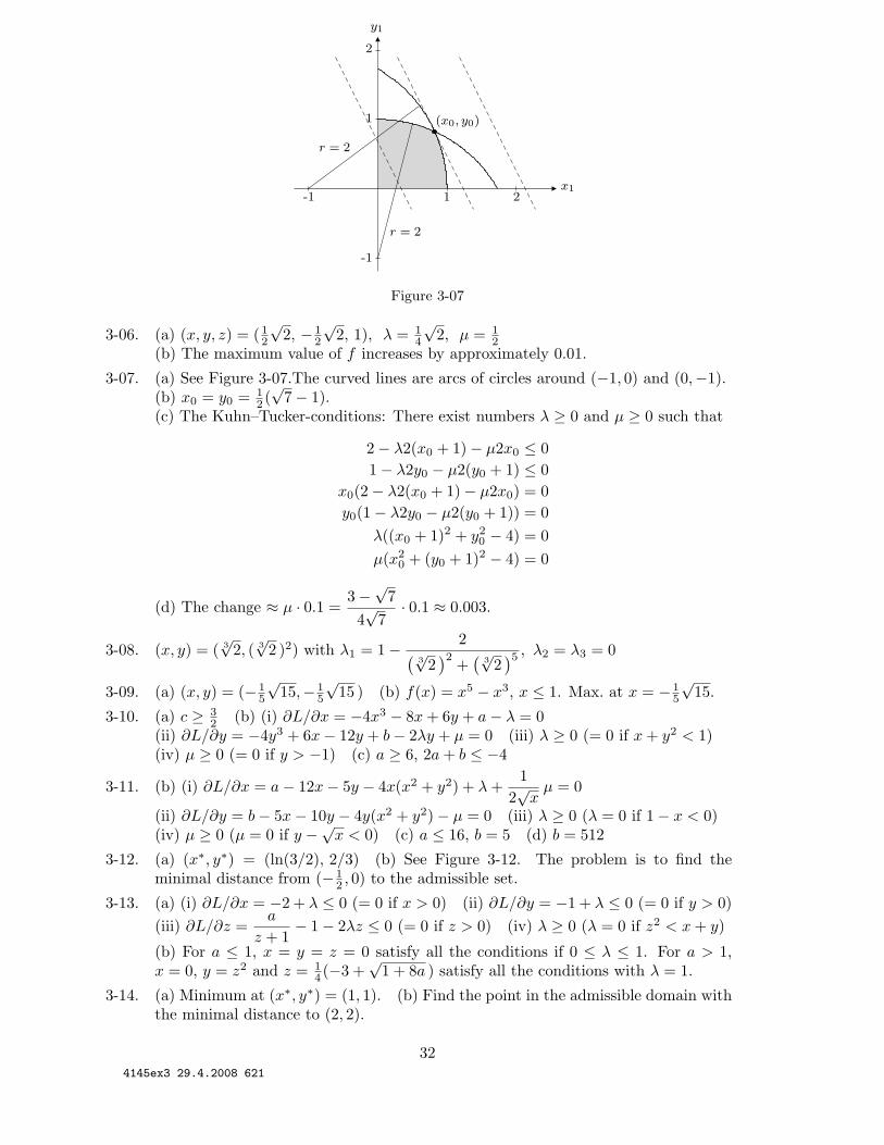
3-07. (a) See Figure 3-07.The curved lines are arcs of circles around (−1, 0) and (0,−1).(b) x0 = y0 = 1

2 (√

7 − 1).(c) The Kuhn–Tucker-conditions: There exist numbers λ ≥ 0 and μ ≥ 0 such that

2 − λ2(x0 + 1) − μ2x0 ≤ 01 − λ2y0 − μ2(y0 + 1) ≤ 0

x0(2 − λ2(x0 + 1) − μ2x0) = 0y0(1 − λ2y0 − μ2(y0 + 1)) = 0

λ((x0 + 1)2 + y20 − 4) = 0

μ(x20 + (y0 + 1)2 − 4) = 0

(d) The change ≈ μ · 0.1 =3 − √

74√

7· 0.1 ≈ 0.003.

3-08. (x, y) = ( 3√

2, ( 3√

2 )2) with λ1 = 1 − 2(3√

2)2 +

(3√

2)5 , λ2 = λ3 = 0

3-09. (a) (x, y) = (− 15

√15,− 1

5

√15 ) (b) f(x) = x5 − x3, x ≤ 1. Max. at x = − 1

5

√15.

3-10. (a) c ≥ 32 (b) (i) ∂L/∂x = −4x3 − 8x + 6y + a − λ = 0

(ii) ∂L/∂y = −4y3 + 6x − 12y + b − 2λy + μ = 0 (iii) λ ≥ 0 (= 0 if x + y2 < 1)(iv) μ ≥ 0 (= 0 if y > −1) (c) a ≥ 6, 2a + b ≤ −4

3-11. (b) (i) ∂L/∂x = a − 12x − 5y − 4x(x2 + y2) + λ +1

2√

xμ = 0

(ii) ∂L/∂y = b − 5x − 10y − 4y(x2 + y2) − μ = 0 (iii) λ ≥ 0 (λ = 0 if 1 − x < 0)(iv) μ ≥ 0 (μ = 0 if y − √

x < 0) (c) a ≤ 16, b = 5 (d) b = 512

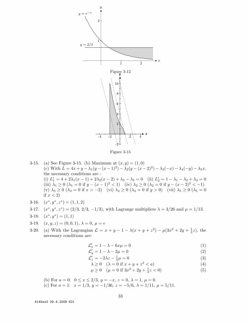
3-12. (a) (x∗, y∗) = (ln(3/2), 2/3) (b) See Figure 3-12. The problem is to find theminimal distance from (− 1

2 , 0) to the admissible set.

3-13. (a) (i) ∂L/∂x = −2 + λ ≤ 0 (= 0 if x > 0) (ii) ∂L/∂y = −1 + λ ≤ 0 (= 0 if y > 0)(iii) ∂L/∂z =

a

z + 1− 1 − 2λz ≤ 0 (= 0 if z > 0) (iv) λ ≥ 0 (λ = 0 if z2 < x + y)

(b) For a ≤ 1, x = y = z = 0 satisfy all the conditions if 0 ≤ λ ≤ 1. For a > 1,x = 0, y = z2 and z = 1

4 (−3 +√

1 + 8a ) satisfy all the conditions with λ = 1.

3-14. (a) Minimum at (x∗, y∗) = (1, 1). (b) Find the point in the admissible domain withthe minimal distance to (2, 2).

324145ex3 29.4.2008 621

y

1

2

x1 2

y = 2/3

y = e−x

Figure 3-12y

-2

2

4

6

8

10

x-4 -2 2 4

y

x

Figure 3-15

3-15. (a) See Figure 3-15. (b) Maximum at (x, y) = (1, 0)(c) With L = 4x + y − λ1(y − (x − 1)2) − λ2(y − (x − 2)2) − λ3(−x) − λ4(−y) − λ5x,the necessary conditions are :(i) L′

1 = 4 + 2λ1(x − 1) + 2λ2(x − 2) + λ3 − λ5 = 0 (ii) L′2 = 1 − λ1 − λ2 + λ4 = 0

(iii) λ1 ≥ 0 (λ1 = 0 if y − (x − 1)2 < 1) (iv) λ2 ≥ 0 (λ2 = 0 if y − (x − 2)2 < −1)(v) λ3 ≥ 0 (λ3 = 0 if x > −2) (vi) λ4 ≥ 0 (λ4 = 0 if y > 0) (vii) λ5 ≥ 0 (λ5 = 0if x < 2)

3-16. (x∗, y∗, z∗) = (1, 1, 2)

3-17. (x∗, y∗, z∗) = (2/3, 2/3, −1/3), with Lagrange multipliers λ = 3/26 and μ = 1/13.

3-18. (x∗, y∗) = (1, 1)

3-19. (x, y, z) = (0, 0, 1), λ = 0, μ = e

3-20. (a) With the Lagrangian L = x + y − 1 − λ(x + y + z2) − μ(3x2 + 2y + 13z), the

necessary conditions are:

L′x = 1 − λ − 6xμ = 0 (1)

L′y = 1 − λ − 2μ = 0 (2)

L′z = −2λz − 1

3μ = 0 (3)λ ≥ 0 (λ = 0 if x + y + z2 < a) (4)μ ≥ 0 (μ = 0 if 3x2 + 2y + 1

3z < 0) (5)

(b) For a = 0: 0 ≤ x ≤ 2/3, y = −x, z = 0, λ = 1, μ = 0.(c) For a = 1: x = 1/3, y = −1/36, z = −5/6, λ = 1/11, μ = 5/11.

334145ex3 29.4.2008 621

y

x2

2

d

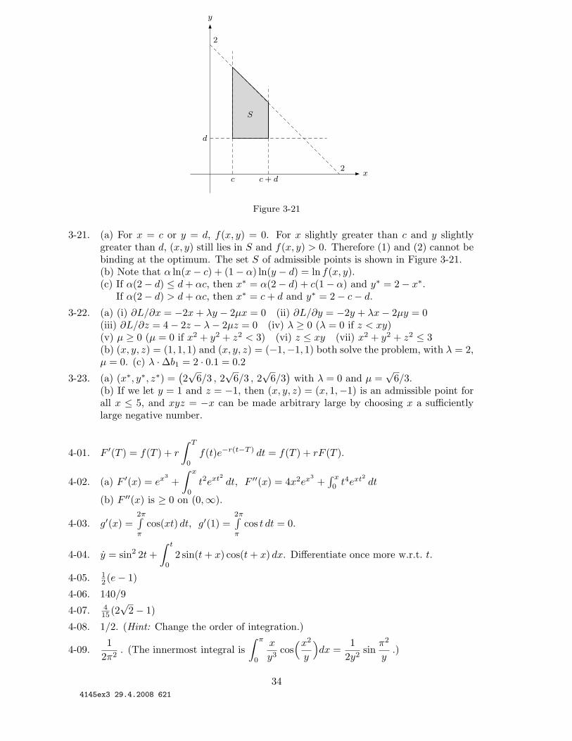
c c + d

S

Figure 3-21

3-21. (a) For x = c or y = d, f(x, y) = 0. For x slightly greater than c and y slightlygreater than d, (x, y) still lies in S and f(x, y) > 0. Therefore (1) and (2) cannot bebinding at the optimum. The set S of admissible points is shown in Figure 3-21.(b) Note that α ln(x − c) + (1 − α) ln(y − d) = ln f(x, y).(c) If α(2 − d) ≤ d + αc, then x∗ = α(2 − d) + c(1 − α) and y∗ = 2 − x∗.

If α(2 − d) > d + αc, then x∗ = c + d and y∗ = 2 − c − d.

3-22. (a) (i) ∂L/∂x = −2x + λy − 2μx = 0 (ii) ∂L/∂y = −2y + λx − 2μy = 0(iii) ∂L/∂z = 4 − 2z − λ − 2μz = 0 (iv) λ ≥ 0 (λ = 0 if z < xy)(v) μ ≥ 0 (μ = 0 if x2 + y2 + z2 < 3) (vi) z ≤ xy (vii) x2 + y2 + z2 ≤ 3(b) (x, y, z) = (1, 1, 1) and (x, y, z) = (−1,−1, 1) both solve the problem, with λ = 2,μ = 0. (c) λ · Δb1 = 2 · 0.1 = 0.2

3-23. (a) (x∗, y∗, z∗) =(2√

6/3 , 2√

6/3 , 2√

6/3)

with λ = 0 and μ =√

6/3.(b) If we let y = 1 and z = −1, then (x, y, z) = (x, 1,−1) is an admissible point forall x ≤ 5, and xyz = −x can be made arbitrary large by choosing x a sufficientlylarge negative number.

4-01. F ′(T ) = f(T ) + r

∫ T

0f(t)e−r(t−T ) dt = f(T ) + rF (T ).

4-02. (a) F ′(x) = ex3+∫ x

0t2ext2 dt, F ′′(x) = 4x2ex3

+∫ x

0 t4ext2 dt

(b) F ′′(x) is ≥ 0 on (0,∞).

4-03. g′(x) =2π∫π

cos(xt) dt, g′(1) =2π∫π

cos t dt = 0.

4-04. y = sin2 2t +∫ t

02 sin(t + x) cos(t + x) dx. Differentiate once more w.r.t. t.

4-05. 12 (e − 1)

4-06. 140/9

4-07. 415 (2

√2 − 1)

4-08. 1/2. (Hint: Change the order of integration.)

4-09.1

2π2 . (The innermost integral is∫ π

0

x

y3 cos(x2

y

)dx =

12y2 sin

π2

y.)

344145ex3 29.4.2008 621

4-10. V ′(t) =∫ t

1F (t, x, t) dx +

∫ t

1F (t, t, y) dy +

∫ t

1

(∫ t

1

∂F (t, x, y)∂t

dx)

dy

4-11.dT (t)

dt=

z(t)x(t + T (t))

− 1,dT (t)

dt=

y(t)y(t + T (t))

− 1

5-01. (a) x = 15 (2e−4t + 3et)

(b) x = 13 ln(6√

t + 8 − 18 ln(3 +√

t + 8 ) + C), C = 18 ln 6 − 17.

5-02. The solution is given implicitly by3

5a2 (ax + b)5/3 − 3b

2a2 (ax + b)2/3 =13t3 + C,

where C is a constant. The left-hand side of this equation can also be written as3x

2a(ax + b)2/3 − 9

10a2 (ax + b)5/3 or3

10a2 (ax + b)2/3(2ax − 3b). The differential

equation also has the constant solution x ≡ −b/a (provided b �= 0).5-03. x(t) = 1 − 2/(t2 − 1)

5-04. (a) x(t) = 2e−2t − e−4t (b) k(t) =(k0 +

a

α

)e(2αs/3)[(t+1)3/2−1] − a

α5-05. (a) x = Ce−2t + 1. (b) w(t) = −e−2t + t + 1.

5-06. (a) K = γKα(βt + L0) (b) K =((1 − α)γ

(β2 t2 + L0t

)+ K1−α

0

)1/(1−α)

5-07. x = Ce−3t + 13 t2 − 2

9 t + 227

5-08. x = 5√

3e−t + 1, x(0) = −15/4

5-09. x =( 4

ϕ(t)2− 9)1/3

, where ϕ(t) = t ln t − t + 2/3.

5-10. x = 12

[3t2 cos(t2) − 3 sin(t2) + 1

]−1/3 − 12 .

5-11. x = et2−2t(3 − 2√

2 + 2√

1 + et )

5-12. x(t) = − 12e1−t3 + 1

2et2−t3

5-13. (a) x = C(t + 1)2 (b) Differential equation for u: u = 2(t + 1)−2 + (t + 1)2. Thegeneral solution of (∗): x = C(t + 1)2 − 2(t + 1) + 1

3 (t + 1)5.

5-14. x = −1 ± (Ae6t + 13 )−1/2 or x ≡ −1.

6-01. (a) x = C1e8t + C2 + 17t/8 (b) x = e−t(A sin 2t + B cos 2t)

6-02. (a) x = C1e−4t + C2e

12 t (b) x = C1e

−4t + C2e12 t − 1

2 t − 78 − 12

85 sin t − 1485 cos t

6-03. (i) x = C1e2t + C2e

7t/4 (ii) x = C1e2t + C2e

7t/4 + 114 t + 15

196 + 265 sin t + 3

65 cos t

6-04. x(t) = e3t(A cos 4t + B sin 4t) + 125 t + 6

625

6-05. x = C1e−3t + C2e

−t/3 + u∗(t) with (i) u∗(t) = 0, (ii) u∗(t) = −2e−t + 2,(iii) u∗(t) = te−3t.

6-06. x = e−t/2(

C1 cos(√

72

t)

+ C2 sin(√

72

t))

+t2

2− t

2+

34

6-07. (i) x = Aer1t + Ber2t, r1,2 = 12a ±

√14a2 − a + 2

(ii) x = Aer1t + Ber2t +t

a − 2+

a

(a − 2)2

6-08. (i) g(t) = Ae−t/4 + B (ii) g(t) = C/(t + 1) + D

6-09. (a) Y ∗ = − 1l + m

t is a particular solution. (b) Y = e−t/2(A cos t + B sin t) − 320 t.

(c) Oscillations if 14 (αl + β)2 < αβ(l + m). For every solution Y we then have

Y (t) +1

l + mt → 0 as t → ∞, that is, Y will approach the linear function Y ∗.

354145ex3 29.4.2008 621

6-10. (a) V (x) = Axa1 + Bxa2 , where a1,2 = −( μ

σ2 − 12

)±√( μ

σ2 − 12

)2+

2ρ

σ2 .

(b) V ∗(x) =1

ρ − μx − w

ρ(c) V (x) = Ax2 +

B

x2 +13x − 5

26-11. (a) x = Aer1t + Ber2t with r1,2 = k − 1 ± √

5 − 2k for k < 52 ,

x = Ae(3/2)t + Bte(3/2)t for k = 52 ,

x = e(k−1)t(A cos

√2k − 5 t + B sin

√2k − 5 t

)for k > 5

2 .

(b) For k �= 2, k �= 5/2: u∗ =1

2k2 − 9k + 10e(4−k)t. For k = 2: u∗ = te2t.

For k = 5/2: u∗ = t2e3t/2.(c) x = e2t(sin t − cos t) + et. t = 0 is a local minimum point.

6-12. (a) Use Leibniz’s rule. (b) p∗ =a + c

b + d. If D = 1

4α2 − β(b + d) > 0 and r1,2 =

− 12α±√

D, then p(t) = C1er1t +C2e

r2t +p∗. If D = 0, p(t) = (C1 +C2t)e−αt/2 +p∗.If D < 0 and γ =

√−D, p(t) = e−αt/2(C1 cos γt + C2 sin γt) + p∗.(c) Oscillations if and only if D = 1

4α2 − β(b + d) < 0.

6-13. (a) x =12At +

B

t(b) x(t) = t

6-14. If k �= −5, x = Ae−5t + Bte−5t + 5(k+5)2 ekt + 6

169 sin t − 5338 cos t.

For k = −5, x = Ae−5t + Bte−5t + 52 t2e−5t + 6

169 sin t − 5338 cos t.

6-15. (a) x = e−2t(A cos 3t + B sin 3t) + 150e2t.

(b) Look for a particular integral of the form C sin 3t + D cos 3t.

7-01. x − 3x + 3x = 1 − 2t. x = e3t/2(C1 cos

√3

2t + C2 sin

√3

2t)

− 2t

3− 1

3,

y = e3t/2(C1 + C2

√3

2cos

√3

2t +

C2 − C1√

32

sin√

32

t)

− t

3− 1

3.

7-02. (a) For a �= ±2,

x = Ae(a−2)t + Be(a+2)t +2β − aα

a2 − 4, y = −Ae(a−2)t + Be(a+2)t +

2α − aβ

a2 − 4.

For a = 2, x = A + Be4t + 12 (α − β)t, y = −A + Be4t − 1

2 (α − β)t − 14 (α + β).

For a = −2, x = Ae−4t + B + 12 (α + β)t, y = −Ae−4t + B + 1

2 (α + β)t + 14 (β − α).

(b) (x∗, y∗) =(2β − aα

a2 − 4,

2α − aβ

a2 − 4

). If a < −2, (x∗, y∗) is (globally) asymptotically

stable. If −2 < a < 2, (x∗, y∗) is a saddle point. (c) x = e−3t + 2, y = −e−3t + 3

7-03. (a) (−1, 0): no decision; (0, 0): no decision; (1,−2): saddle point.(b) x(t) = 1/(t + 1), y(t) = −1/(t + 1)

7-04. (a) (0, 0) is a saddle point; (1/2, 1/2) is locally asymptotically stable.(b) z = z − z2; z = Aet/(1 + Aet) or z ≡ 1. (c) (i) x(t) = y(t) = et/(2et − 1),(ii) x(t) = y(t) = et/(2 + 2et), (iii) x(t) = y(t) = et/(2et − 3).

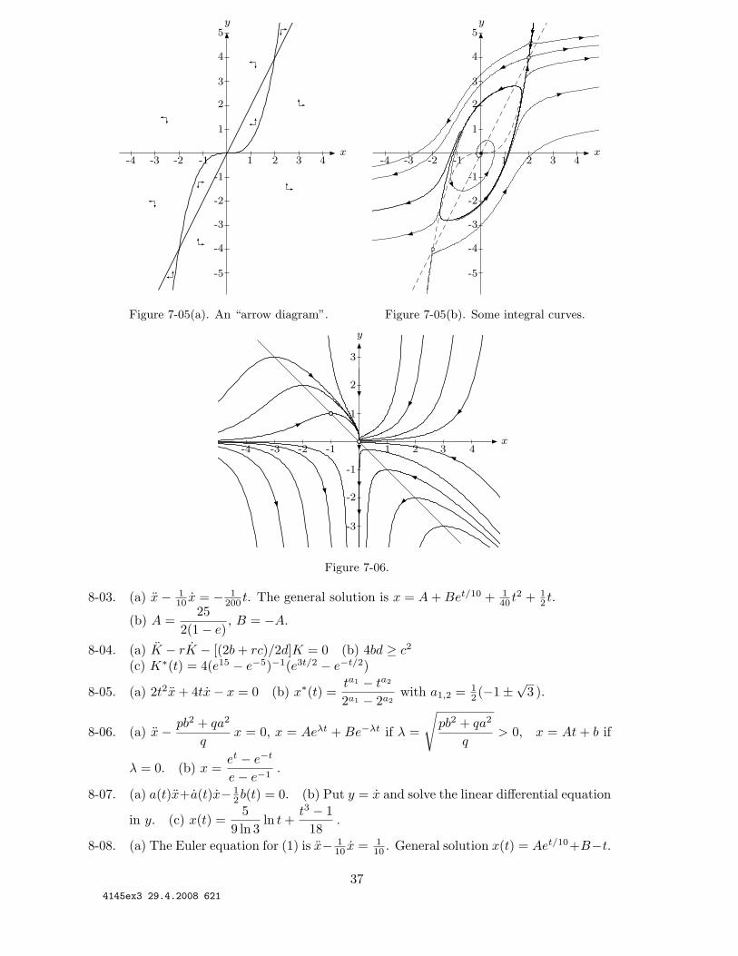
7-05. (a) (0, 0) is a locally asymptotically stable equilibrium point. (2, 4) and (−2,−4)are saddle points. (b) See Figure 7-05(a) and (b). (c) 1

2 (7 +√

41 ) ≈ 6.702.

7-06. (a) See Figure 7-06. (b) The only equilibrium point is (0, 0). Not stable.(c) x(t) = −e−t, y(t) = (z(t))−1, where z(t) = ee−t

(e−1 +∫ t

0 e−e−τ

dτ).(x(t), y(t)) → (0, 0) as t → ∞.

8-01. (a) x = −e−t (b) x = −e−t + e−1 · t + 1

8-02. The Euler equation is x − 4x − 5x = −2e−t. Solution: x∗ = 13 (5 + t)e−t

364145ex3 29.4.2008 621

y

-5

-4

-3

-2

-1

1

2

3

4

5

x-4 -3 -2 -1 1 2 3 4

y

-5

-4

-3

-2

-1

1

2

3

4

5

x-4 -3 -2 -1 1 2 3 4

Figure 7-05(a). An “arrow diagram”. Figure 7-05(b). Some integral curves.

y

-3

-2

-1

1

2

3

x-4 -3 -2 -1 1 2 3 4

Figure 7-06.

8-03. (a) x − 110 x = − 1

200 t. The general solution is x = A + Bet/10 + 140 t2 + 1

2 t.

(b) A =25

2(1 − e), B = −A.

8-04. (a) K − rK − [(2b + rc)/2d]K = 0 (b) 4bd ≥ c2

(c) K∗(t) = 4(e15 − e−5)−1(e3t/2 − e−t/2)

8-05. (a) 2t2x + 4tx − x = 0 (b) x∗(t) =ta1 − ta2

2a1 − 2a2with a1,2 = 1

2 (−1 ± √3 ).

8-06. (a) x − pb2 + qa2

qx = 0, x = Aeλt + Be−λt if λ =

√pb2 + qa2

q> 0, x = At + b if

λ = 0. (b) x =et − e−t

e − e−1 .

8-07. (a) a(t)x+a(t)x− 12b(t) = 0. (b) Put y = x and solve the linear differential equation

in y. (c) x(t) =5

9 ln 3ln t +

t3 − 118

.

8-08. (a) The Euler equation for (1) is x− 110 x = 1

10 . General solution x(t) = Aet/10+B−t.

374145ex3 29.4.2008 621

Solution of the problem: x = 1 − t. (b) x − (β − r)x = − 12a(α − r)e(α−β)t.

8-09. (a) The Euler equation is x ≡ 0, and the solution is x∗(t) ≡ 1. (c) Yes.

8-10. (a) g′′(x)x − rg′(x) − c(t) = 0 (b) x =(B +

T

r

) ert − 1erT − 1

− t

r

(c) x(t) ≥ 0 for t in [ 0, T ] ⇐⇒ Br2 ≥ erT − 1 − rT

9-01. x∗(t) = − 12αe2−t+ 5

2α +5et+ 12αe2+t− 5

2αet, p(t) = 2e2−t−2, u∗(t) = 12α (p(t)−3)

9-02. (a) Necessary conditions:(1) u = u∗(t) maximizes H = −(x∗(t) − u + 2)2e−rt + p(t)(u − δx∗(t)) for u in R,

(2) p(t) = −∂H∗

∂x= 2(x∗(t) − u∗(t) + 2)e−rt + δp(t),

(3) x∗(t) = u∗(t) − δx∗(t), x∗(0) = x0, x∗(T ) = xT .(c) u∗(t) = Be0.5t − 2 − 1

18Ae−0.4t, x∗(t) = Be0.5t − 4 − 59Ae−0.4t,

p(t) = Ae−0.5t, where A =36(3 − e5)5(e5 − e−4)

, B =4(3 − e−4)e5 − e−4 .

9-03. (a) u∗(t) = 12 (e2−t − 1), x∗(t) = 1

4 (e2+t − e2−t) − 12 (et − 1), p(t) = e2−t − 1

(b) x∗(t) ={

et − 1 if 0 ≤ t ≤ t∗,et − 1

4e2−t − 94et−2 + 1

2 if t∗ ≤ t ≤ 2,with t∗ = 2 − ln 3.

9-04. (a) u∗(t) =225

e3/4 − 1e0.15t, x∗(t) =

1500e3/4 − 1

(e0.15t − 1

), p(t) =

1350e3/4 − 1

.

(b) (i) u = u∗(t) maximizes[−C(u, t)e−rt + p(t)u

]for u ≥ 0,

(ii) p(t) = −∂H∗/∂x = 0, (iii) p(5) ≥ 0 (= 0 if x∗(5) > 1500).(c) u∗(t) = 300, x∗(t) = 300t, p(t) = g′(300).

9-05. (a) a ≤ 0, c ≤ 0 and ac − b2 ≥ 0 (b) x − rx − [(a + br)/c]x = 12 (dr/c)t2 − (d/c)t

(c)e3t − e−3t

3(e3 − e−3)− t

39-06. (a) (1) u = u∗(t) maximizes 2(x∗(t))2 − 1

2u2 + p(t)u for u in (−∞,∞),(2) p(t) = −4x∗(t), p(T ) = 0.(b) u∗(t) = p(t) = 2(cos 2t − sin 2t), x∗(t) = sin 2t + cos 2t(c) The maximum principle gives the same suggestion as in (a), but no optimalcontrol exists. (For the suggested control the objective function tends to infinity asc tends to infinity.)

9-07. (a) (i) u = u∗(t) maximizes (p(t) − x∗(t))x∗(t)u for u in [0, 1](ii) p(t) = −2(1 − u∗(t))x∗(t) − p(t)u∗(t) (iii) p(T ) = 0 (iv) x∗(t) = u∗(t)x∗(t)(c) For t ∈ [0, t∗] = [0, T − 1

2 ], we have u∗(t) = 1, x∗(t) = et, p(t) = e2t∗−t.For t ∈ (t∗, T ] = (T − 1

2 , T ] we have u∗(t) = 0, x∗(t) = et∗, p(t) = 2(T − t)et∗

.9-08. (a) (1) I = I∗(t) maximizes −cI2 + λI for I in R,

(2) λ(t) − rλ(t) = −a + 2bK∗(t) + δλ(t), (3) λ(T ) = 0.(b) K∗ − rK∗ − (δ(δ + r) + b/c

)K∗ = −a/2c

(c) K∗(t) = Ae−0.1t + Be0.3t + 20, A =5e − 80e4

4e4 + 1, B = −(A + 20) =

5e + 204e4 + 1

.

(d) We have the same differential equation for K as in part (c), and with the sameinitial condition, K(0) = 0, so once again K∗(t) = Ce−0.1t − (C + 20)e0.3t + 20for a suitable constant C. However, the transversality condition is now λ(10) = e2.(With S(t, K) = Ke0.2t, we have S′

2(t, K) = e0.2t and so S′2(10, K(10)) = e2.)

Hence, K∗(10) + 0.02K∗(10) = 120 . This equation determines the value of C.

9-09. (a) The adjoint function is p(t) = 1 − et−T , and u∗(t) = 1 if ap(t) > e2t, u∗(t) = 0if ap(t) < e2t.

384145ex3 29.4.2008 621

(b) t ≤ ln 2 =⇒ u∗(t) = 1 and x∗(t) = 10e−t − 5e−2t,t > ln 2 =⇒ u∗(t) = 0 and x∗(t) = (15/2)e−t.

(c) u∗(t) ≡ 0, x∗(t) = 5e−t.

9-10. (b) x(t) = 1 − 13 t, u = 2

3 − 13 t

9-11. u∗(t) ={

1 if t ≤ 1,0 if t > 1, x∗(t) =

{t + 1 if t ≤ 1,1 if t > 1, y∗(t) =

{t if t ≤ 1,1 if t > 1, p1(t) =

2 − t, p2(t) = −1/2.

9-12. u = 0, x = 0 for t in [0, 1]; u = 1, x = t − 1 for t in (1, 2].

9-13. (a) (i) u = u∗(t) maximizes(x∗(t)

)2 − x∗(t) + p(t)u for u in [0, 1],(ii) p(t) = −∂H∗/∂x = −2x∗(t) + 1, p(T ) = 0.(b) Solution: For T < 3

2 : u∗(t) = 0, x∗(t) = 0, p(t) = t − T .For T ≥ 3

2 : u∗(t) = 1, x∗(t) = t, p(t) = −t2 + t + T 2 − T .

9-14. (a) For b ≥ a(eT − 1): u∗(t) = 0, x∗(t) = x0et and p(t) = a(eT−t − 1).

For b < a(eT − 1): u∗(t) = 2, x∗(t) = (x0 + 2)et − 2 and p(t) = a(eT−t − 1) in [0, t∗],while u∗(t) = 0, x∗(t) = (x0 + 2)et − 2et−t∗

and p(t) = a(eT−t − 1) in (t∗, T ], wheret∗ = T − ln(1 + b/a).

9-15. u∗(t) = 1, x∗(t) =1√

1 − 2t, p(t) = 12

√11(1 − 2t)3/2 + 46t − 23 if t ∈ [0, 7/22],

u∗(t) = 0, x∗(t) = 12

√11, p(t) = 8 − 24t if t ∈ (7/22, 1/3].

9-16. u∗(t) ={

1 if 0 ≤ t ≤ 1,−1 if 1 < t ≤ 2, x∗(t) =

{t if 0 ≤ t ≤ 1,2 − t if 1 < t ≤ 2.

9-17. u∗(t) =1

C − t, x∗(t) = t − 1

2(C − t)+

12C

, p(t) = C − t, with C = 12 (1 +

√3 )

(b) u∗(t) ={ 1

A−t if t > A − 11 if t ≤ A − 1

, x∗(t) =

{t − 1

2(A−t) + 1 − 12A if t > A − 1

12 t if t ≤ A − 1

,

with A = 12 (5 − √

5 ).

10-01. xt = (√

10 )t(A cos(θt) + B sin(θt)), with cos θ = −3√

10/10.

10-02. x(t) = 5t(C1 cos θt + C2 sin θt) + 120 with cos θ = 3

5 .

10-03. xt = A(−3)t + B 2t + 124 5t − 1

4 t − 316

10-04. xt = 2t − 2(−6)t − t2 − 2t − 2.

10-05. (a) xt = A 2t + B( 1

2

)t + 4 · 3t. If x0 = 0 and x1 = 2, then A = − 163 , B = 4

3 .

(b) xt = A αt + B α−t − βK

αβ2 − (1 + α2)β + αβt

10-06. (a) For c = 0: xt = 25 (−2)t + 3

53t. For c = 1: xt = 715 (−2)t + 7

10 3t − 16 .

(b) We obtain the equation from part (a) with c = 0, x0 = 1 and x1 = 1, andyt = 3

5 (−(−2)t + 3t).

11-01. (a) JT (x) = −x2, with u∗T (x) undetermined. JT−1(x) = −x2/2 with u∗

T−1 = −x/2.JT−2(x) = −x2/3 with u∗

T−2 = −x/3.(b) We claim that JT−k = −x2/(k + 1) with u∗

T−k = −x/(k + 1). This is truefor k = 1. Suppose it is true for k = s. Then JT−(s+1)(x) = maxu∈R(−u2 +JT−s(x + u)) = maxu∈R(−u2 − (x + u)2/(k + 1)). The maximizer for the g(u) =−u2 − (x + u)2/(k + 1) is u = −x/(s + 2). (Note that g is concave.) It follows thatJT−(s+1)(x) = −u2 − (x + u)2/(k + 1) = −x2/(s + 2), which is the given formula fort = s + 1. It follows by induction that the suggested formula is valid for all k.

394145ex3 29.4.2008 621

11-02. (a) JT (x) = x with u∗T (x) = 0, JT−1(x) = 2x with u∗

T−1(x) undetermined, JT−2(x)=3x + 1 with u∗

T−2(x) = 1, JT−3(x) = 4x + 3 with u∗T−3(x) = 1, JT−4(x) = 5x + 6

with u∗T−4(x) = 1

(b) JT−k(x) = (k + 1)x + 12k(k − 1) with u∗

T−k(x) = 1 for k ≥ 2.11-03. (a) JT (x) = lnx with u∗

T (x) undetermined. JT−1(x) = 2 ln(x/2) with u∗T−1 = x/2.

JT−2(x) = 3 ln(x/3) with u∗T−2 = x/3. (b) u∗

T−k = x/(k + 1)11-04. (a) JT (x) = 2x2 for u∗

T (x) = 1. JT−1(x) = 3x2 for u∗T−1 = 0.

(JT−1(x) = maxu∈[0,1]{x2(1+u)+JT (x(1−u))} = x2 maxu∈[0,1](1+u+2(1−u)2}.The function to be maximized is convex in u and has its maximum 3x2 at u = 0.)JT−2(x) = 4x2 with u∗

T−2 = 0.(b) x∗

t = x0 for all t and u∗t = 0 for t = 0, . . . , T − 1, u∗

T = 1. The maximum valueof the objective function is J0(x0) = (T + 2)x2

0.11-05. (a) f0(s, x, u) =

√u for s < T , f0(T, x, u) = −x.

JT (x) = maxu∈(0,∞)(−x) = −x, with u∗T (x) undetermined.

JT−1(x) = maxu∈(0,∞){√

u + JT

(2(x + u)

)}= maxu∈(0,∞) {√

u − 2(x + u)}.Put gT−1(u) =

√u − 2x − 2u. Then g′

T−1(u) = 1/2√

u − 2 = 0 for u = 1/16,and g′′

T−1(u) = −1/4u√

u < 0 for u > 0, so u = 1/16 is the maximizer, andJT−1(x) = −2x + 1/23 for u∗

T−1(x) = 1/24.JT−2(x) = maxu∈(0,∞)

{√u+JT−1

(2(x+u)

)}= maxu∈(0,∞)

{√u−4x−4u+ 1

23

}. It

is easy to see that the function gT−2(u) =√

u−4x−4u+1/23 attains its maximumfor u = 1/26, and JT−2(x) = −22x + (22 − 1)/24 for u∗

T−2 = 1/26.(b) JT−k(x) = −2kx + (2k − 1)/2k+2, by induction.

11-06. (a) JT (x) = maxu∈(0,1](x + lnu) = x for u∗T (x) = 1. JT−1(x) = maxu∈(0,1](x +

lnu + JT (x − u)) = maxu∈(0,1](2x + lnu − u). The maximum is attained at u = 1,so JT−1(x) = 2x − 1 for u∗

T−1(x) = 1. Further, JT−2(x) = maxu∈(0,1](x + lnu +JT−1(x − u)) = maxu∈(0,1](3x + lnu − 2u − 1). We see that JT−2(x) = 3x − 2 − ln 2for u∗

T−1(x) = 1/2.(b) Suppose the formula is valid for t = s. Then JT−(s+1)(x) = maxu∈(0,1](x +lnu + JT−s(x − u)) = maxu∈(0,1](x + lnu + (s + 1)(x − u) − s − ln(1 · 2 · · · s). Wesee that the maximizer is u = 1/(s + 1), and it follows easily that JT−(s+1)(x) =(s + 2)x − (s + 1) − ln(1 · 2 · · · s · (s + 1)), which is the given formula for t = s + 1.

11-07. (a) JT (x) =√

x with u∗T (x) undetermined. JT−1(x) =

√5√

x with u∗T−1 = 4/5.

JT−2(x) = 3√

x with u∗T−2 = 4/9. (b) Inserting Jt(x) = kt

√x into the fundamental

equation and cancelling√

x yields kt−1 = maxu∈[0,1]{2√

u+kt

√1 − u}. The optimal

choice of u is u = 4/(k2t + 4), and it follows that kt−1 =

√k2

t + 4. (Note that withkT = 1, kT−1 =

√5 and kT−2 = 3.)

404145ex3 29.4.2008 621

Date post:	12-Feb-2018
Category:	Documents
Upload:	vuxuyen
View:	262 times
Download:	14 times

EXAM PROBLEMS IN ECON4140/4145 … PROBLEMS IN ECON4140/4145 MATHEMATICS 3 DIFFERENTIAL EQUATIONS,...

Documents