Face Recognition: face in video, age invariance, and facial marks By Unsang Park A DISSERTATION Submitted to Michigan State University in partial fulfillment of the requirements for the degree of DOCTOR OF PHILOSOPHY Computer Science 2009
Transcript
Face Recognition: face in video, age invariance,
and facial marks
By
Unsang Park
A DISSERTATION
Submitted toMichigan State University
in partial fulfillment of the requirementsfor the degree of
DOCTOR OF PHILOSOPHY
Computer Science
2009
Abstract
Face Recognition: face in video, age invariance, andfacial marks
By
Unsang Park
Automatic face recognition has been extensively studied over the past decades
in various domains (e.g., 2D, 3D, and video) resulting in a dramatic improvement.
However, face recognition performance severely degrades under pose, lighting and
expression variations, occlusion, and aging. Pose and lighting variations along with
low image resolutions are major sources of degradation of face recognition performance
in surveillance video.
We propose a video-based face recognition framework using 3D face modeling
and Pan-Tilt-Zoom (PTZ) cameras to overcome the pose/lighting variations and low
resolution problems. We propose a 3D aging modeling technique and show how it can
be used to compensate for age variations to improve face recognition performance.
The aging modeling technique adapts view invariant 3D face models to the given 2D
face aging database. We also propose an automatic facial mark detection method
and a fusion scheme that combines the facial mark matching with a commercial face
recognition matcher. The proposed approach can be used i) as an indexing scheme
for a face image retrieval system and ii) to augment global facial features to improve
the recognition performance.
Experimental results show i) high recognition accuracy (>99%) on a large scale
video data (>200 subjects), ii) ∼10% improvement in recognition accuracy using the
proposed aging model, and iii) ∼0.94% improvement in the recognition accuracy by
utilizing facial marks.
Dedicated to my sweet heart, son, and parents.
iii
Acknowledgments
This is one of the most important and pleasing moments in my life; making a mile
stone in one of the longest project, the PhD thesis. It has been a really long time and
finally I am on the verge of graduating. This could have not been possible without
all the academic and private supports around me.
I would like to thank Dr. Anil K. Jain for giving me the research opportunity in
face recognition. He has always inspired me with all the interesting and challenging
problems. He showed not only which problems we need to solve but how effectively
and how efficiently. I am still working with him as a postdoc and still learning all the
valuable academic practices. I thank Dr. George C. Stockman for raising a number
of interesting questions in my research in face recognition. I always thank him as
my former MS advisor also. I thank Dr. Rong Jin for his guidance in the aspect of
machine learning to improve some of the approaches used in face recognition. I thank
Dr. Yiying Tong for his advice and co-work in all the meetings for the age invariant
face recognition work. I thank Dr Lalita Udpa for joining the committee at the last
moment and reviewing my PhD work.
I thank Greggorie P. Michaud who has provided the Michigan mugshot database
that greatly helped in the facial mark study. I thank Dr. Tsuhan Chen for providing
us the Face In Action database for my work in video based face recognition. I thank
Dr. Mario Savvides for providing the efficient AAM tool for fast landmark detection. I
thank Dr. Karl Jr. Ricanek for providing us the MORPH database in timely manner.
I also would like to thank organizations and individuals who were responsible for
making FERET and FG-NET databases available.
I would like to thank former graduates of PRIP lab; Dr. Arun Ross, Dr. Umut
Uludag, Dr. Hiu Chung Law, Dr. Karthik Nandakumar, Dr. Hong Chen, Dr. Xi-
iv
aoguang Lu, Dr. Dirk Joel Luchini Colbry, Meltem Demirkus, Stephen Krawczyk,
and Yi Chen. I would like to thank all current Prippies; Abhishek Nagar, Pavan Ku-
mar Mallapragada, Brendan Klare, Serhat Bucak, Soweon Yoon, Alessandra Paulino,
Kien Nguyen, Rayshawn Holbrook, Serhat Bucak, and Nick Gregg. They have helped
me in some computer or programming problems, providing their own biometric data,
or giving jokes and sharing each other’s company.
I finally thank to my parents for supporting my study. I thank my mother-in-law
and father-in-law. I thank my wife Jung-Eun Lee for supporting me for the last 7
year’s of marriage. I thank my son, Andrew Chan-Jong Park for giving me happy
1.7 Images of the same subject at age (a) 5, (b) 10, (c) 16, (d) 19, and (e)29 [4]. . . . . . . . . . . . . . . . . . . . . . . . . . . . . . . . . . . . 10
1.8 Four frames from a video: number of pixels between the eyes is ∼45 [37]. 13
1.9 Example face images from a surveillance video: number of pixels be-tween eyes is less than ten and the facial pose is severely off-frontal [5]. 14
1.10 A 3D face model and its 2D projections. . . . . . . . . . . . . . . . . 16
2.1 Schematic of the proposed face recognition system in video. . . . . . . 24
2.2 Pose variations in probe images and the pose values where matchingsucceeds at rank-one: red circles represent pose values where Face-VACS succeeds. . . . . . . . . . . . . . . . . . . . . . . . . . . . . . . 25
2.3 Pose variations in probe images and the pose values where matchingsucceeds at rank-one: red circles represent pose values where PCAsucceeds. . . . . . . . . . . . . . . . . . . . . . . . . . . . . . . . . . . 26
2.4 Example images from the Face In Action (FIA) database. Six differentcameras record the face images at the same time. Six images at threetime instances are shown here. The frontal view at a close distance(fifth image from top to bottom, left to right) is used in the experiments. 29
ix
2.5 Example of face image cropping based on the feature points. (a) Faceimages with AAM feature points and (b) corresponding cropped faceimages. . . . . . . . . . . . . . . . . . . . . . . . . . . . . . . . . . . . 30
2.7 Pose distribution in yaw-pitch space in (a) gallery and (b) probe data. 37
2.8 Face recognition performance on two different gallery data sets: (i) ran-dom gallery: random selection of pose and motion blur, (ii) composedgallery: frames selected based on specific pose and with no motion blur. 39
2.9 Cumulative matching scores using dynamic information (pose and mo-tion blur) for Correlation matcher. . . . . . . . . . . . . . . . . . . . 40
2.10 Cumulative matching scores using dynamic information (pose and mo-tion blur) for PCA matcher. . . . . . . . . . . . . . . . . . . . . . . . 41
2.11 Cumulative matching scores using dynamic information (pose and mo-tion blur) for FaceVACS matcher. . . . . . . . . . . . . . . . . . . . . 41
2.18 Cumulative matching scores by fusing multiple face matchers and mul-tiple frames in near-frontal pose range (-20◦≤ (yaw & pitch) < 20◦). 45
2.19 Proposed face recognition system with 3D model reconstruction andfrontal view synthesis. . . . . . . . . . . . . . . . . . . . . . . . . . . 49
x
2.20 Texture mapping. (a) typical video sequence used for the 3D recon-struction; (b) single frame with triangular meshes; (c) two frames withtriangular meshes; (d) reconstructed 3D face model with one texturemapping from (b); (e) reconstructed 3D face model with two texturemappings from (c). The two frontal poses in (d) and (e) are correctlyidentified in the matching experiment. . . . . . . . . . . . . . . . . . 50
2.21 RMS error between the reconstructed shape and true model. . . . . . 52
2.22 RMS error between the reconstructed and ideal rotation matrix, Ms. 53
2.23 Examples where 3D face reconstruction failed. (a), (b), (c), and (d)show the failure of feature point detection using AAM; (e), (f), and(g) show failures due to deficiency of motion cue. The resulting recon-struction of the 3D face model is shown in (h). . . . . . . . . . . . . . 54
2.24 Face recognition performance with 3D face modeling. . . . . . . . . . 55
2.25 3D model-based face recognition results on six subjects (Subject IDsin the FIA database are 47, 56, 85, 133, 198, and 208). (a) Input videoframes; (b), (c) and (d) reconstructed 3D face models at right view,left view, and frontal view, respectively; (e) frontal images enrolled inthe gallery database. All the frames in (a) are not correctly identified,while the synthetic frontal views in (d) obtained from the reconstructed3D models are correctly identified for the first five subjects, and notfor the last subject (# 208). The reconstructed 3D model of the lastsubject appears very different from the gallery image, resulting in therecognition failure. . . . . . . . . . . . . . . . . . . . . . . . . . . . . 56
2.26 Proposed surveillance system. The ViSE is a bridge between the humanoperator and a surveillance camera system. . . . . . . . . . . . . . . . 58
2.28 Intra- and inter-camera variations of observed color values. (a) originalcolor values, (b) observed color values from camera 1, (c) camera 2,and (d) camera 3 at three different time instances. . . . . . . . . . . . 65
2.33 Example of motion blur. Example close-up image: (a) without motionblur and (b) with motion blur. . . . . . . . . . . . . . . . . . . . . . 71
xi
2.34 Parallel vs. perspective projection. (a) face image captured at a dis-tance of ∼10m, (b) parallel projection of the 3D model, (c) face imagescaptured at a distance of ∼1m (f) perspective projection of the 3D model. 72
2.35 Effect of projection model on face recognition performance. . . . . . 73
2.36 Face recognition performance with static and close-up views. . . . . . 74
2.37 Face recognition performance using real and synthetic gallery imagesand multiple frames. . . . . . . . . . . . . . . . . . . . . . . . . . . . 75
3.1 Example images in (a) FG-NET and (b) MORPH databases. Multi-ple images of one subject in each of the two databases are shown atdifferent ages. The age value is given below each image. . . . . . . . . 80
3.2 3D model fitting process using the reduced morphable model. . . . . 88
3.3 Four example images with manually labeled 68 points (blue) and theautomatically recovered 13 points (red) for the forehead region. . . . 89
3.5 Aging simulation from age x to y. . . . . . . . . . . . . . . . . . . . . 92
3.6 An example aging simulation in FG-NET database. . . . . . . . . . . 95
3.7 Example aging simulation process in MORPH database. . . . . . . . 96
3.8 Example images showing different face cropping methods: (a) originalimage, (b) no-forehead and no pose correction, (c) forehead and nopose correction, (d) forehead and pose correction. . . . . . . . . . . . 99
3.9 Cumulative Match Characteristic (CMC) curves with different meth-ods of face cropping and shape & texture modeling. . . . . . . . . . 100
3.10 Cumulative Match Characteristic (CMC) curves showing the perfor-mance gain based on the proposed aging model. . . . . . . . . . . . . 102
3.11 Rank-one identification accuracies for each probe and gallery agegroups: (a) before aging simulation, (b) after aging simulation, and(c) the amount of improvement after aging simulation. . . . . . . . . 103
xii
3.12 Example matching results before and after aging simulation for sevendifferent subjects: (a) probe, (b) pose-corrected probe, (c) age-adjustedprobe, (d) pose-corrected gallery and (e) gallery. All the images in (b)failed to match with the corresponding images in (d) but images in(c) were successfully matched to the corresponding images in (d) forthe first five subjects. Matching for the last two subjects failed bothbefore and after aging simulation. The ages of (probe, gallery) pairsare (0,18), (0,9), (4,14), (3,20), (30,54), (0,7), and (23,31), respectively,from the top to bottom row. . . . . . . . . . . . . . . . . . . . . . . . 109
3.13 Example matching results before and after aging simulation for fourdifferent subjects: (a) probe, (b) pose-corrected probe, (c) age-adjustedprobe, (d) pose-corrected gallery and (e) gallery. All the images in (b)succeeded to match with the corresponding images in (d) but imagesin (c) failed to match to the corresponding images in (d). The ages of(probe, gallery) pairs are (2,7), (4,9), (7,18), and (24,45), respectively,from the top to bottom row. . . . . . . . . . . . . . . . . . . . . . . . 110
4.2 Two face images of the same person. A leading commercial face recog-nition engine failed to match these images at rank-1. There are a fewprominent facial marks that can be used to make a better decision. . 114
4.3 Three different types of example queries and retrieval results: (a) fullface, (b) partial face, and (c) non-frontal face (from video). The markthat is used in the retrieval is enclosed with a red circle. . . . . . . . 115
4.5 Statistics of facial marks based on a database of 426 images in FERETdatabase. Distributions of facial mark types on mean face and thepercentage of each mark types is shown. . . . . . . . . . . . . . . . . 117
4.6 Effects of generic and user specific masks on facial mark detection. TPincreases and both FN and FP decrease by using user specific mask. . 118
4.7 Schematic of automatic facial mark extraction process. . . . . . . . . 120
4.8 Ground truth and automatically detected facial marks for four imagesin our database. . . . . . . . . . . . . . . . . . . . . . . . . . . . . . . 121
4.9 Schematic of the definitions of precision and recall. . . . . . . . . . . 122
4.10 Precision and recall curve of the proposed facial mark detection method.123
xiii
4.11 An example face image pair that did not match correctly at rank-1 using FaceVACS but matched correctly after fusion for the groundtruth (probe) to automatic marks (gallery) matching. Colored (black)boxes represent matched (unmatched) marks . . . . . . . . . . . . . . 125
4.12 First three rows show three example face image pairs that did notmatch correctly at rank-1 using FaceVACS but matched correctly afterfusion for the ground truth (probe) to ground truth (gallery) matching.Colored (black) boxes represent matched (unmatched) marks. Fourthrow shows an example that matched correctly with FaceVACS butfailed to match after fusion. The failed case shows zero matching scorein mark based matching due to the error in facial landmark detection. 126
xiv
Chapter 1
Introduction
Face recognition is the ability to establish a subject’s identity based on facial char-
acteristics. Automated face recognition requires various techniques from different
research fields, including computer vision, image processing, pattern recognition, and
machine learning. In a typical face recognition system, face images from a number
of subjects are enrolled into the system as gallery data, and the face image of a test
subject (probe image) is matched to the gallery data using a one-to-one or one-to-
many scheme. The one-to-one and one-to-many matchings are called verification and
identification, respectively.
Face recognition is one of the fundamental methods used by human beings to
interact with each other. Attempts to match faces using a pair of photographs dates
back to 1871 in a British court [96]. Techniques for automatic face recognition have
been developed over the past three decades for the purpose of automatic person
recognition with still and video images.
Face recognition has a wide range of applications, including law enforcement, civil
applications, and surveillance systems. Face recognition applications have also been
extended to smart home systems where the recognition of the human face and expres-
sion is used for better interactive communications between human and machines [63].
Fig. 1.1 shows some biometric applications using the face.
The face has several advantages that makes it one of the most preferred biometric
1
(a) (b)
(c) (d)
Figure 1.1. Example applications using face biometric: (a) ID cards (from [1]), (b) facematching and retrieval (from [2]), (c) access control (from [2]), and (d) DynaVox EyeMaxsystem (controlled by eye gaze and blinking, from [3]).
2
traits. First, the face biometric is easy to capture even at a long distance. Second,
the face conveys not only the identity but also the internal feelings (emotion) of the
subject (e.g., happiness or sadness) and the person’s age. This makes face recognition
an important topic in human computer interaction as well as person recognition.
The face biometric is affected by a number of intrinsic (e.g., expression and age)
and extrinsic (e.g., pose and lighting) variations. While there has been a significant
improvement in face recognition performance during the past decade, it is still below
acceptable levels for use in many applications [63] [90]. Recent efforts have focused on
using 3D models, video input, and different features (e.g., skin texture) to overcome
the performance bottleneck in 2D still face recognition. This chapter begins with a
survey of face recognition in 2D, 3D, and video domains and presents the challenges
in face recognition problems. We also introduce problems in face recognition due to
subject aging. The relevance of facial marks or micro features (e.g., scars, birthmarks)
to face recognition is also presented.
1.1 Face Detection
The first problem that needs to be addressed in face recognition is face detec-
tion [131] [21] [132]. Some of the well-known face detection approaches can
be categorized as: i) color based [47], ii) template based [28], and iii) feature
based [103] [123] [44] [61] [127]. Color based approaches learn the statistical model
of skin color and use it to segment face candidates in an image. Template based
approaches use templates that represent the general face appearance, and use cross
correlation based methods to find face candidates. State-of-the-art face detection
methods are based on local features and machine learning based binary classification
(e.g., face versus non-face) methods, following the seminal work by Viola et al. [123].
The face detector proposed by Viola et al. has been widely used in various stud-
ies involving face recognition because of its real-time capability, high accuracy, and
3
Figure 1.2. Example face detection result (from [123]).
availability in the Open Computer Vision Library (OpenCV) [6]. Fig. 1.2 shows an
example face detection result using the method in [123].
1.2 Face Recognition
In a typical face recognition scenario, face images from a number of subjects are
enrolled into the system as gallery data, and the face image of a test subject (probe
image) is matched to gallery data using a one-to-one or one-to-many scheme. There
are three different modalities that are used in face recognition applications: 2D, 3D,
4
Table 1.1. Face recognition scenarios in 2D domain.
ProbeGallery
Single still image Many still images
Single still image one-to-one one-to-many
Many still images many-to-one many-to-many
and video. We will review the face recognition problems in these domains in the
following sections.
1.3 Face Recognition in 2D
Face recognition has been well studied using 2D still images for over a
decade [118] [55] [135]. In 2D still image based face recognition systems, a snap-
shot of a user is acquired and compared with a gallery of snapshots to establish a
person’s identity. In this procedure, the user is expected to be cooperative and pro-
vide a frontal face image under uniform lighting conditions with a simple background
to enable the capture and segmentation of a high quality face image. However, it is
now well known that small variations in pose and lighting can drastically degrade the
performance of the single-shot 2D image based face recognition systems [63]. 2D face
recognition is usually categorized according to the number of images used in matching
as shown in Table 1.1.
Some of the well-known algorithms for 2D face recognition are based on Principle
Component Analysis (PCA) [118] [55], Linear Discriminant Analysis (LDA) [33],
Elastic Graph Bunch Model (EGBM) [126], and correlation based matching [62].
2D face recognition technology is evolving continuously. In the Face Recognition
Vendor Test (FRVT) 2002 [90], identification accuracy of around 70% was achieved
given near frontal pose and normal lighting conditions on a large database (121,589
images from 37,437 subjects, Fig. 1.3). The FRVT 2006 evaluations were performed in
5
a verification scenario and the best performing system showed a 0.01 False Reject Rate
(FRR) at a False Accept Rate (FAR) of 0.001 (Fig. 1.4) given high resolution (400
pixels between eyes1) 2D images (by Neven Vision [7]) or 3D images (by Viisage2 [8]).
Face recognition can be performed in open set or closed set scenarios. Closed set
recognition tests always have the probe subject enrolled in the gallery data, but the
open set recognition consider the possibility that the probe subject is not enrolled
in the gallery. Therefore, a threshold value (on match score) is typically used in
retrieving candidate matches in open set recognition tests [108].
Figure 1.3. Face recognition performance in FRVT 2002 (Snapshot of computerscreen) [90].
1Even though the image resolution is also defined as dots-per-inch (dpi) or pixels-per-inch (ppi),they are effective when the image is printed. Since the digital image is only represented as a set ofpixels when it is processed by a computer, we will use the number of pixels as the measure of imageresolution. Number of pixels between the centers of the eyes was used as the measure of imageresolution in FRVT 2006 [92].
2Now L-1 Identity Solutions.
6
Figure 1.4. Reduction in face recognition error rates from 1993 to 2006 (Snapshot ofcomputer screen) [92].
1.3.1 Challenges in 2D Face recognition
More efforts have been devoted to 2D face recognition because of the availability of
commodity 2D cameras and deployment opportunities in many security scenarios.
However, 2D face recognition is susceptible to a variety of factors encountered in
practice, such as pose and lighting variations, expression variations, age variations,
and facial occlusions. Fig. 1.5 and Fig. 1.6 show examples of the pose and light-
ing variations and occlusion. Local feature based recognition has been proposed to
overcome the global variations from pose and lighting changes [113] [133] [14]. The
use of multiple frames with temporal coherence in a video [136] [10] and 3D face
7
models [17] [71] have also been proposed to improve the recognition rate.
Figure 1.5. Example images showing pose, lighting, and expression variations.
(a) glasses (b) sunglasses (c) hat (d) scarf
Figure 1.6. Example images showing occlusions.
1.3.2 Pose Variation
Pose variation is one of the major sources of performance degradation in face recogni-
tion [63]. The face is a 3D object that appears different depending on which direction
the face is imaged. Thus, it is possible that images taken at two different view points
of the same subject (intra-user variation) may appear more different than two images
taken from the same view point for two different subjects (inter-user variation).
8
1.3.3 Lighting Variation
It has been shown that the difference in face images of the same person due to severe
lighting variation can be more significant than the difference in face images of different
persons [134]. Since the face is a 3D object, different lighting sources can generate
various illumination conditions and shadings. There have been studies to develop
invariant facial features that are robust against lighting variations, and to learn and
compensate for the lighting variations using prior knowledge of lighting sources based
on training data [134] [22] [97]. These methods provide visually enhanced face images
after lighting normalization and show improved recognition accuracy of up to 100%.
1.3.4 Occlusion
Face images often appear occluded by other objects or by the face itself (i.e., self-
occlusion), especially in surveillance videos. Most of the commercial face recognition
engines reject an input image when the eyes cannot be detected. Local feature based
methods are proposed to overcome the occlusion problem [73] [46].
1.3.5 Expression
Facial expression is an internal variation that causes large intra-class variation. There
are some local feature based approaches [73] and 3D model based approaches [52] [70]
designed to handle the expression problem. On the other hand, the recognition of
facial expressions is an active research area in human computer interaction and com-
munications [23].
1.3.6 Age Variation
The effect of aging on face recognition performance has not been substantially studied.
There are a number of reasons that explain the lack of studies on aging effects:
9
• Pose and lighting variations are more critical factors degrading face recognition
performance.
• Template update1 can be used as an easy work-around for aging variation.
• There has been no public domain database for studying aging until recently.
Aging related changes on the face appear in a number of different ways: i) wrinkles
and speckles, ii) weight loss and gain, and iii) change in shape of face primitives
(e.g., sagged eyes, cheeks, or mouth). All these aging related variations degrade face
recognition performance. These variations could be learned and artificially introduced
or removed in a face image to improve face recognition performance. Even though it is
possible to update the template images as the subject ages, template updating is not
always possible in cases of i) missing child, ii) screening, and iii) multiple enrollment
problems where subjects are either not available or purposely trying to hide their
identity. Therefore, facial aging has become an important research problem in face
recognition. Fig. 1.7 shows five different images of the same subject taken at different
ages from the FG-NET database [4].
(a) (b) (c) (d) (e)
Figure 1.7. Images of the same subject at age (a) 5, (b) 10, (c) 16, (d) 19, and (e) 29 [4].
1Template update represents updating the enrolled biometric template to reduce the error ratecaused from template aging.
10
1.3.7 Face Representation
Most face recognition techniques use one of two representation approaches: i) local
feature based [72] [87] [126] [113] [133] [14] or ii) holistic based [119] [55] [79] [122].
Local feature based approaches identify local features (e.g., eyes, nose, mouth, or
skin irregularities) in a face and generate a representation based on their geometric
configuration. Holistic approaches localize the face and use the entire face region in
the sensed image to generate a representation. A dimensionality reduction technique
(e.g., PCA) is used for this purpose. Discriminating information present in micro
facial features (e.g., moles or speckles) is usually ignored and considered as noise.
Applying further transformations on the holistic representation is also a common
technique (e.g., LDA). A combination of local and holistic representations has also
been studied [41] [56].
Local feature based approaches can be further categorized as: i) component
based [43] [54], ii) modular [38] [73] [88] [114] [34], and iii) skin detail based [64] [93].
Component based approaches try to identify local facial primitives (e.g., eyes, nose,
and mouth) and either use all or a subset of them to generate features for matching.
Modular approaches subdivide the face region, irrespective of the facial primitives,
to generate a representation. Skin detail based approaches have recently gained at-
tention due to the availability of high resolution (more than 400 pixels between the
eyes) face images. Facial irregularities (e.g., freckles, moles, scars) can be explicitly
or implicitly captured and used for matching in high resolution face images.
1.4 Face Recognition in Video
While conventional face recognition systems mostly rely upon still shot images, there
is a significant interest in developing robust face recognition systems that will ac-
cept video as an input. Face recognition in video has attracted interest due to the
11
widespread deployment of surveillance cameras. The ability to automatically rec-
ognize faces in real time from video will facilitate, among other things, the covert
method of human identification using an existing network of surveillance cameras.
However, face images in video are often in off-frontal poses and can undergo sub-
stantial lighting changes, thereby degrading the performance of most commercial face
recognition systems. Two distinctive characteristics of a video are availability of: i)
multiple frames of the same subjects and ii) temporal information. Multiple frames
ensure a variation of poses, allowing a proper selection of a good quality frame (e.g.,
high quality face image in near-frontal pose) for high recognition performance. The
temporal information in video is regarded as the information embedded in the dy-
namic facial motion in the video. However, it is difficult to determine whether there
is any identity-related information in the facial motion: more work needs to be done
to utilize the temporal information. Some of the work on video based face recognition
is summarized in Table 2.1. By taking advantage of the characteristics of video, the
performance of a face recognition system can be enhanced. Fig. 1.8 shows four frames
in a typical video captured for face recognition studies [37].
1.4.1 Surveillance Video
The general concept of video based face recognition covers all types of face recognition
in any video data. However, face recognition in surveillance video is more challenging
than typical video based face recognition for the following reasons:
• Pose variations: The subject’s cooperation cannot be assumed because of the
covert characteristics of surveillance applications. Also, the cameras are in-
stalled at elevated positions, resulting in a low probability of capturing frontal
face images.
• Lighting variations: Surveillance systems are often installed in outdoor locations
12
Figure 1.8. Four frames from a video: number of pixels between the eyes is ∼45 [37].
where variations in natural lighting (e.g., bright sunlight to cloudy days) and
shadows degrade the face image quality.
• Low resolution: Surveillance systems use a wide field of view to cover a large
physical area. Therefore, the size of the face appearing in the video frames is
small (number of pixels between eyes ≈10).
Due to the difficulties in simultaneously handling all of the above variations in a
surveillance video, for research purposes it is customary to use a set of video data with
a limited number of variations (e.g., pose or lighting variations) [80] [81]. Fig. 1.9
shows a typical surveillance video captured at a security check point at an airport.
There are severe degradations in quality in terms of pose and resolution compared to
Fig. 1.8.
13
Figure 1.9. Example face images from a surveillance video: number of pixels between eyesis less than ten and the facial pose is severely off-frontal [5].
1.4.2 Challenges
The difficulty of face recognition in video depends on the quality of face images in
terms of pose, lighting variations, occlusion, and resolution. The large number of
frames in video also increases the computational burden. Unlike the still shot 2D
image, surveillance video usually contains multiple subjects in a sequence of frames.
Most of the real-time face detectors [123] are able to detect multiple faces in the
given image. A simultaneous detection and recognition can be performed by associ-
ating each face in current frame with face images observed in previous frames. Low
resolution problems have been addressed by adapting super resolution based image
enhancement [53].
1.5 Face Recognition in 3D Domain
3D face recognition methods use the surface geometry of the face [71]. Unlike 2D face
recognition, 3D face recognition is robust against pose and lighting variations due to
the invariance of the 3D shape against these variations. A 3D image captured from
a face by a 3D sensor covers about 120◦ from right end to left end and this is called
a 2.5D image. A full 3D model covering 360◦ of a face is constructed by combining
14
Table 1.2. Face recognition scenarios across 2D and 3D domain.
ProbeGallery
2D images 3D models or 2.5D images
2D images 2D to 2D 2D to 3D
2.5D images 3D to 2D 3D to 3D
multiple (3 to 5) 2.5D scans. The probe is usually a 2.5D image and the gallery
can be either a 2.5D image or a 3D model. Identification can be performed between
two range (depth) images [71] or between a 2D image and the 3D face model [60].
Table 1.2 extends Table 1.1 across 2D and 3D face models.
There also have been many approaches that are based on reconstructed 3D models
from a set of 2D images [36] [17]. The reconstructed 3D model is used to obtain
multiple 2D projection images that are matched with probe images [60]. Alternatively,
the reconstructed 3D model can be used to generate a frontal view of the probe
image with arbitrary pose and lighting conditions; the recognition is performed by
matching the synthesized probe in frontal pose. Fig. 1.10 shows a 3D face model and
its corresponding 2D projection images under different pose and lighting conditions.
1.5.1 Challenges
3D face models are usually represented as a polygonal (e.g., triangular or rectangular)
mesh structure for computational efficiency [83]. The 3D mesh structure changes
depending on the preprocessing (e.g., smoothing, filling holes, etc.), mesh construction
process, and imaging process (scanning with laser sensor). Even though the 3D
geometry of a face model changes depending on the pose, this change is very small and
the model is generally regarded as pose invariant. Similarly, the model is also robust
against lighting variations. However, 3D face recognition is not invariant against
variations in expression, aging, and occlusion. There have been several studies on
15
Figure 1.10. A 3D face model and its 2D projections.
expression invariant 3D face recognition [52] [70] and studies on age variation are
beginning to appear [82] [104]. The drawbacks in 3D face recognition are the large
size of the 3D model, which requires high computation cost in matching, and the
expensive price of 3D imaging sensors.
1.6 Summary
We have reviewed various face recognition schemes with respect to different data
modalities: 2D, video, and 3D. Even though there have been steady improvements
in face recognition performance over the past decade, several challenges remain due
to the large intra-class variations and small inter-class variations. These variations
are mostly due to pose and lighting variations, expression, occlusion, aging, and non-
robust representations of face image data.
16
While 3D face recognition has been studied to overcome pose and lighting prob-
lems, a number of factors have prevented the practical application of 3D face recog-
nition; these include computation cost, sensor cost, and large legacy data in the 2D
domain. Video based face recognition is important for its need in surveillance. How-
ever, the video domain has its own challenging set of problems related to severe pose
and lighting variations and poor resolution. Taking advantage of the rich temporal
information in video and using 3D modeling techniques to assist video based face
recognition has been regarded as a promising approach.
This thesis will focus on three major problems in face recognition. First, we utilize
3D modeling techniques, temporal information in video, and a surveillance camera
setup to improve the performance of video based face recognition. Second, we develop
a framework for age invariant face recognition. Third, we develop a framework for
utilizing secondary local features (e.g., facial marks) as a means of complementing
the primary facial features to improve face matching and retrieval performance.
1.7 Thesis Contributions
We have developed methods to improve face recognition performance in three ways:
i) using temporal information in video, ii) models for facial variations due to aging,
and iii) utilizing secondary features (e.g., facial marks). Contributions of the thesis
are summarized below.
• A systematic method of gallery and probe construction using video data is pro-
posed. The pose and motion blur significantly affect face recognition accuracy.
We perform face recognition in video by selectively using a subset of frames
that are in near frontal pose with small blur. Fusion across multiple frames and
multiple matchers on the selected frames results in high identification accuracy.
• We use 3D modeling techniques to overcome the pose variation problem. The
17
Factorization algorithm [116] is adapted for 3D model reconstruction to synthe-
size frontal views and improve the matching accuracy. The synthesized frontal
face images substantially improve the face recognition performance.
• A multi-camera surveillance system that captures soft-biometric features (e.g.,
height and clothing color) has been developed. The soft biometric information
is coupled with face biometrics to provide robust tracking and identification
capabilities to conventional surveillance systems.
• We propose a pair of static and Pan-Tilt-Zoom (PTZ) cameras to overcome the
low image resolution problem. The static camera is used to locate the face and
the PTZ camera is used to zoom in and track the face image. The close-up view
of the face provides a high resolution face image that substantially improves the
recognition accuracy.
• To address age invariant face recognition systems, we use the Principle Com-
ponent Analysis (PCA) technique to model the shape and texture separately.
The PCA coefficients are estimated from a training database containing mul-
tiple images at different ages from a number of subjects to construct an aging
pattern space. The aging pattern space is used to correct for aging and narrow
down the age separation between probe and gallery images.
• An automatic facial mark detection system is developed that can be used in face
matching and retrieval. We have used an Active Appearance Model (AAM) [26]
to localize and mask primary facial features (e.g., eyes, eye brows, nose, and
mouth). A Laplacian of Gaussian (LOG) operator is then applied on the rest
of the face area to detect facial mark candidates. A fusion of mark based
matching and a commercial matcher shows that the recognition performance
can be improved.
18
Chapter 2
Video-based Face Recognition
Deciding a person’s identity based on a sequence of face images appearing in a video
is called video based face recognition. Unlike still-shot 2D images, video data contains
rich information in multiple frames. However, the pose and lighting variations in a
video are more severe compared with still-shot 2D images. This is mostly because
human subjects are more cooperative in the still-shot image capture process. On the
contrary, most often video data is captured in covert applications and the subject’s
cooperation is not usually expected. Therefore, video based face recognition presents
some additional challenges in face recognition.
There have been a number of studies that perform face recognition specifically on
video streams. Chowdhury et al. [24] estimate the pose and lighting of face images
contained in video frames and compare them against synthetic 3D face models ex-
hibiting similar pose and lighting. However, in their approach the 3D face models
are registered manually with the face image in the video. Lee et al. [59] propose an
appearance manifold based approach where each gallery image is matched against the
appearance manifold obtained from the video. The manifolds are obtained from each
sequence of pose variations. Zhou et al. [136] proposed to obtain statistical models
from video using low level features (e.g., by PCA) contained in sample images. The
matching is performed between a single frame and the video or between two video
streams using the statistical models. Liu et al. [68] and Aggarwal et al. [10] use HMM
19
Table 2.1. A comparison of video based face recognition methods.
Approaches No. ofsubjects indatabase
Recognitionaccuracy
Chowdhury etal. [24]
Frame level matching with synthe-sized gallery from 3D model
32 90%
Lee et al. [59] Matching frames with appearancemanifolds obtained from video
20 92.1%
Zhou etal. [136]
Frame to video and video to videomatching using statistical models
25 (Videoto video)
88∼100%1
Liu et al. [68] Video level matching using HMM 24 99.8%
Aggarwal etal. [10]
Video level matching using Au-toRegressive and Moving Averagemodel (ARMA)
45 90%
1 Four videos are prepared for each subject as the subject is walking slowly, walkingfast, inclining, and carrying an object. Different performances are shown dependingon different selection of probe and gallery video.
20
and ARMA models, respectively, for direct video level matching. Most of these direct
video based approaches provide good performance on small databases, but need to be
evaluated on large databases. Table 2.1 summarizes some of the major video based
recognition methods presented in the literature.
We propose an approach to face recognition in video that utilizes 3D modeling
technique. The proposed method focuses on the utilization of 3D models than the
temporal information embedded in the 2D video; the effectiveness of the proposed
approach is evaluated on a large database (>200 subjects). We utilize the modeling
techniques in view-based and view synthetic approaches to improve the recognition
performance [81] [80].
View-based and view synthesis methods are two well known approaches to over-
come the problem of pose and lighting variations in video based face recognition.
View-based methods enroll multiple face images under various pose and lighting con-
ditions and match the probe image to the gallery image with the most similar pose
from the input probe images with pose and lighting conditions similar to those in
the gallery to improve the matching performance. The desired view can be synthe-
sized by learning the mapping function between pairs of training images [15] or by
using 3D face models [17] [102]. The parameters of the 3D face model in the view
synthesis process can also be used for face recognition [17]. These view-based and
view-synthetic approaches are also applicable to still images. However, considering
the large pose and lighting variations in multiple 2D images taken at different times, it
is more suitable to use these techniques for video data. The view synthesis approach
has the following two advantages over the view based method: i) it does not require
the tedious process of collecting multiple face images under various pose and light-
ing conditions, and ii) it can generate frontal facial images under favorable lighting
conditions on which state-of-the-art face recognition systems can perform very well.
21
However, the view synthesis approach needs to be applied carefully, so that it does
not introduce noise that may further degrade the original face image.
2.1 View-based Recognition
If we assume that a video is available for a subject both for gallery construction at
enrollment and as probe, we can take advantage of video for improving the face recog-
nition performance. In this section we explore (a) the adaptive use of multiple face
matchers in order to enhance the performance of face recognition in video, and (b) the
possibility of appropriately populating the database (gallery) in order to succinctly
capture intra-class variations. To extract the dynamic information in video, the pose
in various frames is explicitly estimated using Active Appearance Model (AAM) and a
Factorization based 3D face reconstruction technique [116]. We also estimate the mo-
tion blur using the Discrete Cosine Transformation (DCT). Our experimental results
on 204 subjects in CMU’s Face-In-Action (FIA) database show that the proposed
recognition method provides consistent improvements in the matching performance
using three different face matchers (e.g., FaceVACS, PCA, and correlation matcher).
2.1.1 Fusion Scheme
Consider a video stream with r frames and assume that the individual frames have
been processed in order to extract the faces present in them. Let T1, T2, . . . , Tr
be the feature sets computed from the faces localized in the r frames. Further,
let W1,W2, . . . , Wn be the n identities enrolled in the authentication system and
G1, G2, . . . , Gn, respectively, be the corresponding feature templates associated with
these identities. The first goal is to determine the identity of the face present in the
ith frame as assessed by the kth matcher. This can be accomplished by comparing
the extracted feature set with all the templates in the database in order to determine
22
the best match and the associated identity. Thus,
IDi = argmaxj=1,2,...,n
Sk(Ti, Gj), (2.1)
where IDi is the identity of the face in the ith frame and Sk(·, ·) represents the
similarity function employed by the kth matcher to compute the match score between
feature sets Ti and Gj . If there are m matchers, then a fusion rule may be employed
to consolidate the m match scores. While there are several fusion rules, we employ
the simple sum rule (with min-max normalization of scores) [50] to consolidate the
match scores, i.e.,
IDi = argmaxj=1,2,...,n
m∑
k=1
Sk(Ti, Gj). (2.2)
In practice, simple fusion rules work as well as complicated fusion rules such as the
likelihood ratio [77].
Now the identity of a subject in the given video stream can be obtained by ac-
cumulating the evidence across the r frames. In frame level fusion, we assume each
frame is equally reliable, so the score sum is used. In matcher level fusion, the com-
mercial matchers usually outperform the public domain matchers. Therefore, we take
the maximum rule that will favorably take the matching score with the highest con-
fidence (e.g., commercial matcher). In maximum rule, the identity that exhibits the
highest match score in the r frames is deemed to be the final identity. Therefore,
ID = argmaxj=1,2,...,n
(argmaxi=1,2,...,r
(m∑
k=1
Sk(Ti, Gj)
)). (2.3)
In the above formulation, it must be noted that the feature sets Ti and Gj are
impacted by several different factors such as facial pose, ambient lighting, motion
blur, etc. If the parameter vector θ denotes a compilation of these factors, then the
feature sets are dependent on this vector, i.e., Ti ≈ Ti(θ) and Gj ≈ Gj(θ). In this
23
Figure 2.1. Schematic of the proposed face recognition system in video.
work, m is 3 since three different face matchers are used and the vector θ represents
facial pose and motion blur in video. The dynamic nature of the fusion rule is
explained in the subsequent sections. Fig. 2.1 shows the overall schematic of the
proposed view-based face recognition system using video.
2.1.2 Face Matchers and Database
Given the large pose variations in video data, it is expected that using multiple
matchers will cover larger pose variations for improved accuracy. Most of the com-
mercial face matchers reject the input image when the facial pose is severely off-frontal
(> 40◦) and both eyes cannot be detected. We use two public domain matchers that
24
−40 −30 −20 −10 0 10 20 30−40
−30
−20
−10
0
10
20
30pose−cognitec
yaw
pitc
h
CognitecOnly Cognitec
Figure 2.2. Pose variations in probe images and the pose values where matching succeedsat rank-one: red circles represent pose values where FaceVACS succeeds.
25
−40 −30 −20 −10 0 10 20 30−40
−30
−20
−10
0
10
20
30pose−pca
yaw
pitc
h
PCAOnly PCA
Figure 2.3. Pose variations in probe images and the pose values where matching succeedsat rank-one: red circles represent pose values where PCA succeeds.
26
can generate a matching score even with failed eye detection to compensate for the
failure of enrollment in the commercial facial matcher. We selected the state-of-the-
art commercial face matcher FaceVACS from Cognitec [9] and two public domain
matchers: PCA [119], and a correlation based matcher [62]. FaceVACS, which per-
formed very well in the Face Recognition Vendor Test (FRVT) 2002 and FRVT 2006
competitions [90] [92], is known to use a variation of Principle Component Analy-
sis (PCA) technique. However, this matcher has limited operating range in terms
of facial pose. To overcome this limitation and facilitate a continuous decision on
the subject’s identity across multiple poses, the conventional PCA [118] [55] based
matcher and a cross correlation based matcher [62] were also considered. The PCA
engine calculates the similarity between probe and gallery images after applying the
Karhunen-Loeve transformation to both the probe and galley images. The cross cor-
relation based matcher calculates the normalized cross correlation between the probe
and gallery images to obtain the matching score. Fig. 2.2 and 2.3 show the differ-
ence in the success of face recognition at different facial poses for two different face
matchers: FaceVACS and PCA. It is shown that these two matchers are successful
for different pose values.
We use CMU’s Face In Action database [37], which includes up to 221 subjects
with data collected in three indoor sessions and three outdoor sessions. Each subject
was recorded by six different cameras simultaneously, at two different distances and
three different angles. The number of subjects varies across these different sessions.
We use the first indoor session in our experiments because it i) has the largest number
of subjects (221), ii) contains a significant number of both frontal and non-frontal
poses, and iii) has relatively small lighting variations. Each video of a subject consists
of 600 frames. We partition the video data into two halves; the first half was used as
gallery data and the second half as probe data. Fig. 2.4 shows example images of the
FIA database. In the FIA database the images captured from six different cameras
27
are stored as separate images. While FIA is now available in the public domain, we
have not found any other face recognition study using this database.
2.1.3 Tracking Feature Points
Facial pose is an important factor to consider in video based face recognition. We
detected and tracked a set of facial feature points and estimated the facial pose using
the reconstructed or generic 3D face models. The Active Appearance Model (AAM)
was used to detect and track facial feature points. The Viola-Jones face detector
[123] was used to locate the face; feature points were rejected when they deviated
substantially from the face area estimated with the face detector. The AAM feature
points were also used to tightly crop the face area to be used by the PCA and
cross correlation matchers. Fig. 2.5 shows example images of AAM tracking and the
resulting cropped face images.
2.1.4 Active Appearance Model (AAM)
The AAM is a statistical model of the facial appearance generated by combining
shape and texture variations [25]. Constructing an AAM requires a set of training
data X={X1, X2, . . . , Xn} with annotations, where Xi represents a set of points
marked on image i. Exact correspondences are required in X across all the n training
images. By applying PCA to X, any Xi can be approximated by
Xi = Xµ + Ps · bsi , (2.4)
where Xµ is the mean shape, Ps is a set of the orthogonal modes of variation obtained
by applying PCA to X, and bsi is a set of shape parameters. To build a texture model,
each example image is warped so that its control points match the mean shape. Then
the face texture g (gray values) is obtained by the region covered by the mean shape.
28
Figure 2.4. Example images from the Face In Action (FIA) database. Six different camerasrecord the face images at the same time. Six images at three time instances are shown here.The frontal view at a close distance (fifth image from top to bottom, left to right) is usedin the experiments.
29
(a)
(b)
Figure 2.5. Example of face image cropping based on the feature points. (a) Face imageswith AAM feature points and (b) corresponding cropped face images.
The texture model is defined similar to the shape model as
gi = gµ + Pg · bgi , (2.5)
where gµ is the mean texture, Pg is a set of orthogonal modes of variation obtained
by applying PCA to g, and bgi is a set of texture parameters. The shape and texture
parameters are combined as b = (bs, bg) and any new face image is approximated by
b. Now the problem becomes finding the best shape and texture parameter vector bi
that achieves the minimum difference between the test image Ii and the image Im
generated by the current model defined by bi. More details about an efficient way of
searching for the best model parameter bi can be found in [25]. There are enhanced
versions of AAM that have real time capability [130] using 2D and 3D information,
and that are robust against occlusions [40]. A user-specific AAM has also been studied
for more robust feature point detection when the user specific model is available [98].
30
2.1.5 AAM Training
Instead of using a single AAM for multiple poses as in Section 2.1.3, we constructed
multiple AAMs, each for a different range of pose variations [27] to cover a larger
set of variations in facial pose. In this way, each model is expected to find better
facial feature points for its designated pose. Moreover, the number of feature points
in each AAM can be different according to the pose (e.g., frontal vs. profile). We
chose seven different AAMs corresponding to frontal, left half profile, left profile, right
half profile, right profile, lower profile, and upper profile poses to cover the observed
pose variations appearing in our video data. Assuming facial symmetry, the right
half and right profile models are obtained from the left half and left profile models,
respectively.
The off-line manual labeling of feature points for each training face image is a time
consuming task. Therefore, we used a semi-automatic training process to build the
AAMs. The training commenced with about 5% of the training data that had been
manually labeled, and the AAM search process was initiated for the unlabeled data.
Training faces with robust feature points were included into the AAM after manually
adjusting the points, if necessary. The AAM facial feature search process was then
initiated again. This process was repeated until all the images in the training set had
been labeled with feature points. Our proposed scheme uses a generic AAM where
the test subject is not included in the trained AAM. To simulate this scenario, we
generated two sets of AAMs and used them in a cross validation way to ensure the
separation between AAM training and testing.
2.1.6 Structure from Motion
Let a set of points Pi = {pi1, pi2, ..., piP } denote the 2D shape of a 3D object S ob-
served in an image Ii. Given a video with F frames, Θ = {I1, I2, ..., IF } containing the
2D projections of the 3D object S, we obtain a sequence of points Π = {P1, P2, ..., PF }.
31
The relationship between S and Pi can be described as
Pi = C · (Ri · S + Ti), (2.6)
where C, R, and T are the camera projection matrix, rotation matrix, and translation
matrix, respectively. The Structure from Motion (SfM) problem can be stated as
estimating S from the observed set of points Pi = {P1, P2, ..., PF }. The challenge in
the SfM problem is to find sets of Pi that correspond in a sequence of video frames.
Due to object and camera motion, some parts of the object are occluded, resulting
in missing and spurious feature points. A solution to SfM involves using the least
squared error method, which tolerates error in feature point detection to a certain
degree.
2.1.7 3D Shape Reconstruction
The Factorization method [116] is a well known solution for the Structure from Motion
problem. There are different factorization methods to recover the detailed 3D shape
depending on the rigidity of the object [129] [19]. We regard the face as a rigid object
and treat small changes in facial expression as noise in feature point detection. This
helps us recover only the most dominant shape from video data. Under orthographic
projection model, the relationship between 2D feature points and 3D shape is given
by
W = M · S, (2.7)
32
W =
u11 u12 . . . u1p
u21 u22 . . . u2p
...
uf1 uf2 . . . ufp
v11 v12 . . . v1p
v21 v22 . . . v2p
...
vf1 vf2 . . . vfp
,
M =
i1x i1y i1z
i2x i2y i2z
...
ifx ify ifz
j1x j1y j1z
j2x j2y j2z
...
jfx jfy jfz
,
S =
Sx1 Sx2 . . . Sxp
Sy1 Sy2 . . . Syp
Sz1 Sz2 . . . Szp
,
(2.8)
where ufp and vfp in W represent the row and column pixel coordinates of the pth
point in the f th frame, each pair of iTf = [ifx ify ifz] and jTf = [jfx jfy jfz] in M
represents the rotation matrix with respect to the f th frame, and S represents the 3D
shape. The translation term is omitted in Eq. (2.7) because all 2D coordinates are
centered at the origin. The rank of W in Eq. (2.8) is 3 in an ideal noise-free case. The
solution of Eq. (2.7) is obtained by a two-step process: (i) Find an initial estimate of
M and S by singular value decomposition, and (ii) apply metric constraints on the
initial estimates. By a singular value decomposition of W, we obtain
W = U ·D · V T ≈ U ′ ·D′ · V ′T , (2.9)
33
where U and V are unitary matrices of size 2F × 2F and P × P , respectively and D
is a matrix of size 2F ×P for F frames and P tracked points. Given U , D and V , U ′
represents the first three columns of U , D′ is the first three columns and first three
rows of D, and V ′T is the first three rows of V T , to impose the rank 3 constraint on
W . Then, M ′ and S′ (the initial estimates of M and S) are obtained as
M ′ = U ′ ·D′1/2,
S′ = D′1/2 · V ′T .(2.10)
To impose the metric constrains on M, a 3× 3 correction matrix A is defined as
([if jf ]T · A) · (AT · [if jf ]) = E, (2.11)
where if is the f th i vector in the upper half rows of M , jf is the f th j vector in the
lower half rows of M , and E is a 2×2 Identity matrix. The constraints in Eq. 2.11
need to be imposed across all frames. There is one if and one jf vector in each frame,
which generate three constraints. Since A ·AT is a 3×3 symmetric matrix, there are
6 unknown variables. Therefore, at least two frames are required to solve Eq. 2.11. In
practice, to obtain a robust solution, we need more than two frames and the solution
is obtained by the least squared error method. The 3×3 symmetric matrix L = A ·AT
with 6 unknown variables is solved first and then L1/2 is calculated to obtain A. The
conditions when factorization fails are: (i) number of frames F is less than 2, (ii)
the singular value decomposition fails, or (iii) L is not positive definite. Usually,
conditions (i) and (ii) are not of concern in processing a video with a large number
of frames. Most of the failures occur due to condition (iii). Therefore, the failure
condition of the factorization process can be determined by observing the positive
definiteness of L through eigenvalue decomposition. The final solution is obtained as
34
M ′ = M ′ · A,
S′ = A−1 · S′, (2.12)
where M contains the rotation information between each frame and the 3D object
and S contains the 3D shape information. We will provide the lower bound on the
performance of the Factorization method on synthetic data and real data in Sec. 2.2.2.
2.1.8 3D Facial Pose Estimation
We estimate the facial pose in a video frame to select the best pose to use in recog-
nition. There are many facial pose estimation methods in 2D and 3D domains [117].
Because the head motion occurs in a 3D domain, 3D information is necessary for
accurate pose estimation. We estimate the facial pose in [yaw, pitch, roll] (YPR)
values as shown in Fig. 2.6. Even though all the rotational relationships between the
3D shape and the 2D feature points in each frame are already established through
the matrix M in the factorization process, it reveals only the first two rows of the ro-
tation matrix for each frame, which generates inaccurate solutions in obtaining YPR
values, especially in noisy data. Moreover, the direct solution cannot be obtained in
cases where the factorization fails. Therefore, we use the gradient descent method
to iteratively fit the reconstructed 3D shape to the 2D facial feature points. The re-
constructed 3D shape is first initialized to zero yaw, pitch, and roll, and the iterative
gradient descent process is applied to minimize the objective function
E = ‖Pf − C ·R · S‖, (2.13)
where Pf is the 2D facial feature points in the f th frame, C is an orthogonal camera
projection matrix, R is the full 3 x 3 rotation matrix, and S is the 3D shape. The
overall process of pose estimation is depicted in Fig. 2.6. The proposed pose estima-
35
tion scheme is evaluated on a synthetic data consisting of 66 frames obtained from a
3D model with known poses. The pose variations in synthetic data are in the range
[−45◦, 45◦] in yaw and pitch. The pose estimation error on the synthetic data is less
than 6o on average. However, this error increases in real face images because of the
noise in the feature point detection process.
Figure 2.6. Pose estimation scheme.
36
−200 −150 −100 −50 0 50 100 150 200−200
−150
−100
−50
0
50
100
150
200Gallery
Yaw
Pitc
h
(a)
−200 −150 −100 −50 0 50 100 150 200−200
−150
−100
−50
0
50
100
150
200Probe
Yaw
Pitc
h
(b)
Figure 2.7. Pose distribution in yaw-pitch space in (a) gallery and (b) probe data.
37
2.1.9 Motion Blur
Unlike still shot images of the face, motion blur is often present in segmented face
images in video. The blurred face images can confound the recognition engine re-
sulting in matching errors. Therefore, frames with motion blur need to be identified
and they either need to be enhanced or rejected in the face recognition process. The
degree of motion blur in a given image can be evaluated based on a frequency do-
main analysis: motion blur decreases the fraction of sharp edges, which are high
frequency components. Any spatial to frequency domain transformation method can
be used to detect the degree of high frequency components (e.g. Fourier transfor-
mation (FT) [39] or Discrete Cosine Transformation (DCT) [11]). We used DCT
to evaluate the degree of high frequency components for its simplicity compared to
FT. DCT is a similar operation as FT, but it uses only real numbers. The N1 ×N2
real numbers x0,0, . . . , xN1−1,N2−1 are transformed into the N1 × N2 real numbers
X0,0, . . . , XN1−1,N2−1 after the DCT transformation defined as
Xk1,k2 =
N1−1∑
n1=0
N2−1∑
n2=0xn1,n2 cos
π(n1 + 1/2)k1N1
cosπ(n2 + 1/2)k2
N2(2.14)
where k1 = 0, . . . , N1 − 1 and k2 = 0, . . . , N2 − 1 . We determined the presence
of motion blur by observing the DCT coefficients of the top 10% of high frequency
components; frames with motion blur were not considered in the adaptive fusion
scheme.
2.1.10 Experimental Results
We performed three different experiments to analyze the effect of i) gallery data,
ii) probe data, and iii) adaptive fusion of multiple matchers on the face recognition
38
1 2 3 4 5 6 7 8 9 100
0.1
0.2
0.3
0.4
0.5
0.6
0.7
0.8
0.9
1
Rank
Cum
ulat
ive
accu
racy
FaceVACS, Composed GalleryFaceVACS, Random GalleryPCA, Composed GalleryPCA, Random GalleryCorrelation, Composed GalleryCorrelation, Random Gallery
Figure 2.8. Face recognition performance on two different gallery data sets: (i) randomgallery: random selection of pose and motion blur, (ii) composed gallery: frames selectedbased on specific pose and with no motion blur.
performance in video. We first report the experimental results as CMC curves at the
frame level. The subject level matching performance is also provided along with the
overall system performance.
To study the effect of gallery composition, we constructed two different gallery
data sets. The first gallery set, A, was constructed by selecting 7 frames per sub-
ject with pitch and yaw values as (−40◦,0◦), (−20◦,0◦), (0◦,0◦), (0◦,20◦), (0◦,40◦),
(0◦,−20◦), (0◦,20◦). These frames are also selected not to have any motion blur.
The second gallery set, B, also has the same number of frames per subject but it
is constructed by considering a random selection of yaw and pitch values, and these
may contain motion blur. The effect of gallery data set on the matching performance
is shown in Fig. 2.8. The gallery database composed by using pose and motion blur
39
information (set A) shows significantly better performance for all the three matchers.
This is because the composed gallery covers larger pose variations appearing in probe
data. Removing images with motion blur also positively affects the performance.
Figure 2.9. Cumulative matching scores using dynamic information (pose and motionblur) for Correlation matcher.
Next, we separate the probe data according to the facial pose in three different
ranges: i) between −20◦ and 20◦, ii) between −40◦ and −20◦ or 20◦ and 40◦, and
iii) between −60◦ and −40◦ or 40◦ and 60◦ for yaw and pitch values. We com-
puted the CMC curves for these three different probe sets as shown in Fig. 2.9∼2.11.
Fig. 2.9∼2.11 indicates that for all the three matchers, the face recognition perfor-
mance is the best in near frontal-view and decreases as it deviates from the frontal
view. Fig. 2.12∼2.17 show the same results as Fig. 2.9∼2.11, but using separate
pitch and yaw information. The overall performance is observed to be slightly lower
with pitch variation compared to yaw. In Figs. 2.12∼2.14, the performance does
not strictly become lower as the pose variation increases. We believe this is due to
40
Figure 2.10. Cumulative matching scores using dynamic information (pose and motionblur) for PCA matcher.
Figure 2.11. Cumulative matching scores using dynamic information (pose and motionblur) for FaceVACS matcher.
41
Figure 2.12. Cumulative Matching Characteristic curves with the effect of pitch for cor-relation matcher.
Figure 2.13. Cumulative Matching Characteristic curves with the effect of pitch for PCAmatcher.
42
Figure 2.14. Cumulative Matching Characteristic curves with the effect of pitch for Face-VACS matcher.
Figure 2.15. Cumulative Matching Characteristic curves with the effect of pitch for cor-relation matcher.
43
Figure 2.16. Cumulative Matching Characteristic curves with the effect of pitch for PCAmatcher.
Figure 2.17. Cumulative Matching Characteristic curves with the effect of pitch for Face-VACS matcher.
Figure 2.18. Cumulative matching scores by fusing multiple face matchers and multipleframes in near-frontal pose range (-20◦≤ (yaw & pitch) < 20◦).
the noise in pose estimation process. Finally, Fig. 2.18 shows the effects of fusion of
multiple matchers and multiple frames using dynamic information of facial pose and
motion blur. We used score-sum with min-max score normalization and max-sum as
described in Sec. 2.1.1. The best rank-1 accuracy by combining all three matchers
achieved 96% accuracy. The frame level fusion result (subject level matching accu-
racy) exhibited over 99% accuracy. Tables 2.2 and 2.3 show examples of matching
results for two of the subjects in the database according to the choice of gallery, probe,
and matcher, where the final fusion with composed gallery shows the best results.
Experiments on view-based face recognition were performed assuming a large num-
ber of images are available both in the probe and gallery data and a subset of the
45
Table 2.2. Face recognition performance according to gallery, probe, and matcher for videoexample 1.
46
Table 2.3. Face recognition performance according to gallery, probe, and matcher for videoexample 2.
47
probe data contains poses that are similar to those in the gallery data. In this case,
it is more important to select gallery and probe images that are close to each other.
However, when none of the probe and gallery data is similar in pose, we need to
synthetically generate probe face images that are close to the gallery images. For this
purpose, we introduce a view-synthetic approach in the following section.
2.2 View-synthetic Face Recognition in Video
The face images of subjects enrolled in a face recognition system are typically in
frontal pose, while the face images observed at recognition time are often non-frontal.
We propose a view-synthetic method to generate the face images that are similar
to the enrolled face images in terms of facial pose. We propose to automatically
(i) reconstruct a 3D face model from multiple non-frontal frames in a video, (ii)
generate a frontal view from the derived 3D model, and (iii) use a commercial 2D face
recognition engine to recognize the synthesized frontal view. A factorization-based
structure from motion algorithm [116] is used for 3D face reconstruction. Obtaining a
3D face model from a sequence of 2D images is an active research problem. Morphable
model (MM) [17], stereography [74], and Structure from Motion (SfM) [120] [116] are
well known methods in 3D face model construction from 2D images or video. While
morphable models have been shown to provide accurate reconstruction performance,
the processing time is overwhelming (4.5 minutes [17]), which precludes their use in
real-time systems. Stereography also provides good performance and has been used
in commercial applications [17], but it requires a pair of calibrated cameras, which
limits its use in many surveillance applications. Structure from motion (SfM) gives
reasonable performance, has the ability to process in real-time, and does not require
a calibration process, making it suitable for surveillance applications. Since we are
focusing on face recognition in surveillance video, we propose to use the SfM technique
to reconstruct the 3D face models as described in Sec. 2.1.6. The overall schematic
48
of the system is depicted in Fig 2.19.
Figure 2.19. Proposed face recognition system with 3D model reconstruction and frontalview synthesis.
2.2.1 Texture Mapping
We define the 3D face model as a set of triangles and generate a Virtual Reality
Modeling Language (VRML) object. Given the 72 feature points obtained from the
reconstruction process, 124 triangles are generated. While the triangles can be ob-
tained automatically by the Delaunay triangulation process [120], we use a predefined
set of triangles for the sake of efficiency because the number and configuration of the
feature points are fixed. The corresponding set of triangles can be obtained from
the video frames with a similar process. Then, the VRML object is generated by
mapping the triangulated texture to the 3D shape. The best frame to be used in tex-
ture mapping is selected based on the pose estimation scheme described in Sec. 2.1.8.
When all the available frames deviate significantly from the frontal pose, two frames
49
are used in the texture mapping as described in Fig. 2.20. Even though both the
synthetic frontal views in Figs. 2.20 (d) and (e) are correctly recognized, the view in
(e) looks more realistic. When more than one texture is used for texture mapping,
a sharp boundary is often observed across the line where two different textures are
combined because of the differences in illumination. However, the synthetic frontal
views are correctly recognized in most cases regardless of this artifact.
Figure 2.20. Texture mapping. (a) typical video sequence used for the 3D reconstruc-tion; (b) single frame with triangular meshes; (c) two frames with triangular meshes; (d)reconstructed 3D face model with one texture mapping from (b); (e) reconstructed 3Dface model with two texture mappings from (c). The two frontal poses in (d) and (e) arecorrectly identified in the matching experiment.
2.2.2 Experimental Results
We performed the following set of three experiments. i) Evaluation of the minimum
requirement of rotation angle and number of frames for the factorization algorithm
both synthetic and real data, ii) 3D face modeling on a public domain video database,
50
and iii) face recognition using the reconstructed 3D face models.
3D Face Reconstruction with Synthetic Data
A set of 72 facial feature points were obtained from the true 3D face model, which
were constructed from the 3D range sensor data. A sequence of 2D coordinates of
the facial feature points were directly obtained from this true model. We took the
angular values for the rotation in steps of 0.1 in the range (0.1,1) and in steps of
1.0 in the range (1,10). The number of frames used was 2, 3, 4, and 5. The Root
Mean Squared (RMS) error between the ground truth and the reconstructed shape is
shown in Fig. 2.22. While the number of frames required for the reconstruction in the
noiseless case is two (see Sec. 2.1.7), in practice more frames are needed to keep the
error small. As long as the number of frames was more than two, the reconstruction
errors were observed to be negligible (≈ 0).
3D Face Reconstruction with Real Data
For real data, noise is present in both the facial feature point detection and the
correspondences between detected points across frames. This noise is not random and
its affect is more pronounced at points of self-occlusion and on the facial boundary,
as observed in Fig. 2.5. Since AAM does use feature points on the facial boundary,
the point correspondences are not very accurate in the presence of self-occlusion.
Reconstruction experiments were performed on real data with face rotation from −45◦
to +45◦ across 61 frames. Example frames from a real video sequence are shown in
Fig. 2.5. We estimated the rotation between successive frames as 1.5◦ (61 frames
varying from −45◦ to +45◦) and obtained the reconstruction error with rotation
in steps of 1.5◦ in the range (1.5◦,15◦). The number of frames used varied from 2
to 61. A direct comparison between the true model and the reconstructed shape
is not possible for real data because the ground truth is not known. The original
51
database was collected only as 2D video and 3D models of the corresponding subjects
were not available. Therefore, we measured the orthogonality of M to estimate the
reconstruction accuracy. Let M be a 2F × 3 matrix as shown in Eq. 2.7 and M(a :
b, c : d) represent the sub matrix of M from rows a to b and columns c to d. Then,
Ms = M × M ′ is a 2F × 2F matrix where all elements in Ms(1 : F, 1 : F ) and
Ms(F + 1 : 2F, F + 1 : 2F ) are equal to 1 and all elements in Ms(1 : F, F + 1 : 2F )
and Ms(F + 1 : 2F, 1 : F ) are equal to 0 if M is truly an orthogonal matrix. We
measured the RMS difference between the ideal Ms and the calculated Ms as the
reconstruction error. The reconstruction error for real data is shown in Fig. 2.22.
Our experiments show that the number of frames needed for reconstruction from real
data is more than the synthetic data, but the error decreases quickly as the number
of frames increases. The increase in error with larger pose difference is due to error
in point correspondences from self-occlusion.
Figure 2.21. RMS error between the reconstructed shape and true model.
52
Figure 2.22. RMS error between the reconstructed and ideal rotation matrix, Ms.
Face Recognition with Pose Correction
We used CMU’s Face In Action (FIA) video database [37] (see Sec. 2.1.2) for our
matching experiments. We used selected frames of the FIA database to simulate the
video observed in a surveillance scenario. To demonstrate the advantage of using
reconstructed 3D face models for recognition, we were primarily interested in video
sequences that contained mostly non-frontal views for each subject. Since the recon-
struction with SfM performs better when there are large motion differences between
frames, both left and right non-frontal views were collected for each subject, if avail-
able, resulting, on average, in about 10 frames per subject (a total of 221 subjects).
When there was sufficient motion difference between frames and the feature point
detector performed well, it was possible to obtain the 3D face model from only 3
53
Figure 2.23. Examples where 3D face reconstruction failed. (a), (b), (c), and (d) show thefailure of feature point detection using AAM; (e), (f), and (g) show failures due to deficiencyof motion cue. The resulting reconstruction of the 3D face model is shown in (h).
different frames, which is consistent with the results shown in Fig. 2.21. The num-
ber of frames that is required for the reconstruction can be determined based on the
orthogonality of M . Typical frames from video sequences are shown in Fig. 2.20 (a).
We successfully reconstructed 3D face models for 207 subjects out of the 221
subjects. The reconstruction process failed for 14 subjects either due to poor facial
feature point detection in the AAM process or the deficiency of motion cue, which
caused a degenerate equation in the factorization algorithm.
Example images where AAM or SfM failed are shown in Fig. 2.23. The recon-
structed 3D face models were corrected in their pose to make all yaw, pitch, and roll
values equal to zero. The frontal face image can be obtained by projecting the 3D
model in the 2D plane. Once the frontal view was synthesized, the FaceVACS face
recognition engine from Cognitec [9] was used to generate the matching score. The
54
1 2 3 4 5 6 7 8 9 100
0.1
0.2
0.3
0.4
0.5
0.6
0.7
0.8
0.9
1
rank
cum
ulat
ive
accu
racy
Frontal video framesNon−frontal video frames with 3D modelingNon−frontal video frames
Figure 2.24. Face recognition performance with 3D face modeling.
face recognition results for frontal face video, non-frontal face video, and non-frontal
face video with 3D face modeling are shown in Fig. 2.24. These results are based on
207 subjects for which the 3D face reconstruction was successful. The CMC curves
show that the FaceVACS engine does extremely well for frontal pose frames but its
performance drops drastically for non-frontal pose frames. By using the proposed
3D face modeling, the rank-1 performance in the non-frontal scenario is improved by
40%. Example 3D face models and the synthesized frontal views from six different
subjects (subject ID: 47, 56, 85, 133, 198, and 208 in the FIA database) are shown
in Fig. 2.25. All these input video frames were incorrectly recognized by the Face-
VACS engine. However, after 3D model reconstruction, the synthetic frontal views
were correctly recognized except for the last subject. The synthetic frontal view of
55
(a) (b) (c) (d) (e)
Figure 2.25. 3D model-based face recognition results on six subjects (Subject IDs in theFIA database are 47, 56, 85, 133, 198, and 208). (a) Input video frames; (b), (c) and(d) reconstructed 3D face models at right view, left view, and frontal view, respectively;(e) frontal images enrolled in the gallery database. All the frames in (a) are not correctlyidentified, while the synthetic frontal views in (d) obtained from the reconstructed 3Dmodels are correctly identified for the first five subjects, and not for the last subject (#208). The reconstructed 3D model of the last subject appears very different from the galleryimage, resulting in the recognition failure.
56
this subject appears sufficiently different from the gallery image, resulting in a false
match.
2.3 Video Surveillance
With increasing security concerns, surveillance cameras have become almost ubiqui-
tous in public and private places. However, most of these surveillance cameras were
initially installed with limited functionalities of providing video streams to human
operators for review after a security breach. In order to assess security threats in
real time and identify subjects in video, development of automated video surveillance
systems is needed.
Many studies on automated surveillance systems that utilize computer vision and
image processing techniques have been reported [30] [128] [51]. The automation
of surveillance systems will not only increase the number of manageable cameras
per operator, but it will also remove the necessity of video recording by identifying
critical events in real-time. With the difficulties encountered in fully automating the
surveillance systems, semi-automatic surveillance systems that can effectively utilize
human intelligence through the interaction with surveillance systems are becoming
mainstream.
Another trend in developing surveillance camera systems is using networked cam-
eras. Networked cameras are installed with built-in ethernet cards and send the
captured video to the Digital Video Recording (DVR) systems through the ethernet
cable. Networked cameras simplify the installation and maintenance processes and,
in turn, enable monitoring large areas, especially when a wireless ethernet is used.
Networked cameras use compressed images due to the limited bandwidth available
in many applications. The noise involved in networked cameras due to the image
compression will be addressed in our image processing algorithms.
We have developed a Visual Search Engine (ViSE) as a semi-automatic component
57
Figure 2.26. Proposed surveillance system. The ViSE is a bridge between the humanoperator and a surveillance camera system.
in a surveillance system using networked cameras. The ViSE aims to assist the
monitoring operation of huge amounts of captured video streams; these operations
find and track people in the video based on their primitive features with the interaction
of a human operator.
In contrast to the conventional viewpoint of partitioning surveillance systems into
human intervention and camera systems, we decompose the surveillance systems into
three different parts: (i) human intervention, (ii) Visual Search Engine (ViSE), and
(iii) conventional camera system. A human operator translates high-level queries such
as “Is this a suspicious person?” or “Where is the person X?” into low-level queries
with primitive (image) features that ViSE can easily understand. The translation of
the query is performed based on the knowledge of the operator. For example, the
best visual features of a missing child can be provided by his parents. Examples of
low-level queries with primitive features are “Show all subjects wearing a blue shirt,”
or “Show all subjects that passed location Y.” For the purpose of finding a person,
ViSE narrows down the candidates and the human operator then chooses the final
target. To be able to interact with human operators, ViSE processes input video
streams and stores primitive features for all the objects of interest in the video. The
58
block diagram of the proposed system is shown in Fig. 2.26.
We address the issues of object detection and tracking, shadow suppression, and
color-based recognition for the proposed system. The experimental results on a set
of video data with ten subjects showed that ViSE retrieves correct candidates with
83% recall at 83% precision.
2.3.1 Moving Object Detection
The first step in processing video input is detecting objects of interest. A well-known
method of object detection is based on the inter-frame subtraction of the current
frame against a reference frame [29] [86] or a few adjacent frames [13].
Moving object detection or motion segmentation is one of the most important
tasks in video surveillance, object tracking, and video compression [76]. The simplest
method of motion extraction is background subtraction [106] [109]. Each image is
compared with the reference background image and the difference between the two
images is extracted. This method is used when the background is static over a
relatively long period of time. In video surveillance, the reference background is
periodically updated. The background subtraction is very simple to implement with
low computational cost, which makes it ideal for real-time processing. However,
keeping the reference image static is not trivial in many situations. The reference is
easily corrupted by a small camera oscillation. In addition, even when the background
is stationary with respect to noisy motion, it is usually not static with respect to
illumination. The illumination change is detected in the background subtraction and
estimated as a motion.
Frame subtraction against past images is used for motion detection when the
reference image is not obtainable. Most frame subtraction techniques use two or
three consecutive frames [13] [48] [105]. The background image is assumed not to
change much across the frames. The detected change in two or three frames is used
59
to retrieve the outline of the moving object. The moving object is segmented from
the outline or further processing is performed to refine the segmentation. The frame
subtraction technique can be used in more general cases than background subtraction
because it does not need a reference image. However, the frame subtraction method
depends on the velocity of the moving object in the image. If the velocity is low, it
cannot be detected, while the segmentation is overestimated if the velocity is high.
Horn and Schunck [45] used a motion constraint equation to analyze motion in a
sequence of images: each pixel in the image is evaluated for its magnitude and direc-
tion of motion. A set of pixels that are correlated with the optical flow is segmented
as one region. The set of pixels with large magnitude of motion corresponds to the
moving object. Optical flow provides more information about the motion in an image
by estimating direction of motion, which allows for more detailed analysis than back-
ground subtraction or frame subtraction. However, the motion between consecutive
frames is assumed to be small in optical flow. The main disadvantage of optical flow
is its high computational cost.
We used the background subtraction method for the moving object detection be-
cause of its capability of real-time processing and detection of slowly moving objects.
Background Subtraction
Conventional background subtraction methods are very sensitive to noise, so they
are not useful in our system, because of the additional noise in networked cameras.
We propose a slight variation of the Gaussian background modeling method. Our
approach estimates the background model both at the pixel level and at the image
level.
Let It(x, y) denote the image captured at time t, and BN = {It(x, y)|t =
1, 2, . . . , N} denote the set of N images used in the background modeling. In a
recursive fashion, the mean µ(x, y) and standard deviation σ(x, y) for each pixel (x,y)
60
can be calculated as
µt =t− 1
tµt−1 +
xn
t, (2.15)
σ2t =
t− 1
tσ2
t−1 +(xt − µt)
2
t− 1, (2.16)
where t = 1, 2, , N . Once µ and σ are estimated, a pixel is declared to be in the
background if
|It(x, y)− µ(x, y)| < k · σ(x, y), (2.17)
and foreground, otherwise. Setting the value of k to 3 implies that we expect the
model will include 99.73% of the background pixels if the distribution of pixel val-
ues is Gaussian. However, due to the violation of Gaussian assumption in practice,
additional noise due to image compression and the limited data in building the back-
ground model, the rule in Eq. (2.17) results in many false classifications of background
pixels as foreground. These false classifications can be suppressed by introducing an
additional threshold in Eq. (2.17), which can be obtained from the secondary mean
and standard deviation computed as
µ′ = 1
nx · ny
∑x,y
σ(x, y) (2.18)
σ′ =√
1
nx · ny
∑x,y
(σ(x, y)− µ′)2, (2.19)
where nx and ny denote the number of rows and columns, respectively. The parame-
ters µ(x, y) and σ(x, y) and µ′ and σ′ account for the background model at the pixel
level and the image level, respectively. The modified criterion to decide a pixel as
background is
|It(x, y)− µ(x, y)| < k · σ + (µ′ + k · σ′). (2.20)
As the camera captures a new frame, the new image Inew(x, y) replaces the old image
61
Iold(x, y) in BN and the background model is updated by recursively updating µ(x, y)
and σ(x, y) as
µnew = µold +new − old
N(2.21)
σ2new = σ2
old +(new − µn)2 − (old− µo)
2
N+
(µn − µo{(new − µn) + (old− µo)}N
,
(2.22)
where the subscript new(n) denotes the newly added pixel values and the subscript
old(o) denotes the pixel values to be removed. The parameters µ′ and σ′ are also
updated from the new I(x, y). By keeping only N images in the buffer and updating
the background model, no false detections due to background changes persist over N
frames, an improvement over other background modeling methods. However, since
part of an object that is static for N frames can be misclassified as background, a
user intervention is also allowed to initialize and update the background model.
Suppression of Shadows
We first perform the proposed background subtraction in RGB space and then remove
shadows from the second pass background subtraction in the Hue-Saturation-Intensity
(HSI) space. The RGB space is better at detecting salient objects, but suffers from
many false positives due to shadows. Therefore, object segmentation using the com-
bination of RGB and HSI space is expected to be more robust in terms of both salient
region detection and shadow suppression. To save computation, first pass subtraction
is performed in I space and second pass subtraction is performed in H and S space.
The second pass subtraction is also performed only on the foreground pixels whose
I value is decreased from the background. The difference between background sub-
traction in V and HS spaces is shown in Fig. 2.27, where I space subtraction shows a
clear background but includes the shadow. The HS space subtraction, on the other
hand, shows the advantage of shadow suppression.
62
Figure 2.27. Background subtraction.
2.3.2 Object Tracking
Homography-based Location Estimation
Homography is a mapping function between two different 2D projection images of a
3D scene [42]. It is well known that the homography between two images requires four
corresponding points. Using this, we transform the 2D motion segmented image into
the 2D representation of the floor (foot) print (i.e., surveillance area) to obtain the
location of the subjects from the top-view. Two base homographic transformations H0
and Hh are calculated from four observed points in the image at two different heights
0 meters and h meters from the ground. Then, the homographic transformation, Hy,
at a height of y meters, 0 ≤ y ≤ h is calculated based on the following interpolation
Hy =(h− y) ·H0 + y ·Hh
h. (2.23)
The location of a person can be estimated by integrating the multiple transformed
planes and detecting the peak value from the integration as
location = argmaxx,z
(∫ h
0Hy · Sdy
), (2.24)
63
where S is a cylindrical object for the convolution operation. This location estimation
method can suppress the segmentation error, such as cracks and holes that are caused
by the additional sources of noise in networked cameras.
Kalman Filter
In accumulating the moving path of a subject, a conventional linear Kalman filter [125]
is used for prediction and smoothing. The Kalman filter can be formulated in the
prediction stage as
xk = Axk−1 + Buk−1 (2.25)
Pk = APk−1AT + Q (2.26)
and in the correction stage as
Kk = PkHT (HPkHT + R)−1, (2.27)
xk = xk + Kk(zk −Hxk), (2.28)
Pk = (I −KkH)Pk, (2.29)
where xk is the predicted state, xk is corrected state with measurement, zk is the
measurement, Q is process noise covariance matrix, R is measurement noise covariance
matrix, A denotes parameters that relate the state from k − 1 to k, B relates u to
the state x, H relates x to z, P is the estimation error covariance matrix, and K is
the Kalman gain.
Primitive Feature Extraction
To enable communication between the human operator and the surveillance system, it
is critical to select descriptive features that can be understood and processed at both
ends. We chose clothing color, height, and build of the subjects as three features that
64
can be easily computed at a distance using networked cameras. In addition, these
three features are easy for human operators to recall to describe a subject because
they are commonly used in the real world. Below we describe how we compute each
of these three features.
Clothing Color
The detected blob corresponding to a person in the video was divided into three parts
from top to bottom (at 1/5th and 3/5th of the person’s height). A combination of the
color values of middle and bottom parts was considered to describe the color feature.
One problem in color matching is that the observed color values in the RGB space
from different cameras vary as much as those observed in different instances from the
same camera as shown in Fig. 2.28.
Figure 2.28. Intra- and inter-camera variations of observed color values. (a) original colorvalues, (b) observed color values from camera 1, (c) camera 2, and (d) camera 3 at threedifferent time instances.
By removing the lightness component (I component) in the HSI color space, the
color variation can be greatly reduced. Saturation also causes variations in color
values from pure to dark but in the same color label. We propose a color-matching
scheme by using hue as the main component with the assistance of saturation and
intensity. The color is decided mainly according to the hue and the possibility of
65
color being white, black, or gray is decided by S and V components. A histogram
with ten bins (red, brown, yellow, green, blue, violet, pink, white, black, and gray)
is constructed from every pixel in the segmented object. The decision threshold for
each color is made from the boundary values in standard color charts. The final color
is decided as the bin with the largest count.
Height
The height of the person is estimated as the y-value at the location of a subject in
Eq. (2.24).
Figure 2.29. Schematic retrieval result using ViSE.
2.3.3 Experimental Results
We collected three instances of video recordings of five different subjects and one
instance of video recording from a different set of five subjects using three networked
cameras installed in a hallway. Durations of the video clips ranged between 25 and 30
seconds with ten frames per second. Since one instance of video recording generates
three video clips from three different cameras, the total number of video clips was
sixty.
We evaluated the performance of ViSE in terms of the accuracy of feature extrac-
tion and the precision and recall for subject retrieval. Given the set of pre-recorded
66
video data with ten different subjects, ViSE showed 93% overall accuracy in color
feature extraction and about 2 cm average deviation in height measurement. At 79%
precision, the recall for subject retrieval was 85% using only the color features. Using
both color and height, the recall was decreased to 83% with an increased precision of
83%. Some example search results using ViSE are shown in Fig. 2.29. It can be seen
that ViSE is able to retrieve correct candidates and, in turn, significantly reduce the
operator’s burden.
The resolution of face images in the video data is very low (∼10 pixels between
the eyes), which made it infeasible to perform face recognition tasks. However, the
extracted soft biometric features can help in improving person identification accuracy
as shown in [49]. To address the low resolution problem in video surveillance, we
propose a face recognition method at a distance in the next section.
Figure 2.30. Schematic of face image capture system at a distance.
67
Figure 2.31. Schematic of camera calibration.
2.4 Face Recognition in Video at a Distance
In typical surveillance application scenarios, the distance between the subject and
camera is large (> 10m) and the resolution of face image is relatively poor (no. of
pixels between eyes < 10) resulting in low recognition performance of face recognition
systems. We propose to use a pair of static and PTZ cameras to obtain higher
resolution face images (no. of pixels between eyes > 100) at a distance of 10 or
more meters. There have been a few studies on face recognition at a distance using
a camera system consisting of static and PTZ cameras [111] [67]. However, most of
the studies are limited in the sense that only tracking is enabled and face recognition
performance is evaluated on a small number of subjects (≤5).
68
2.4.1 Image Acquisition System
To obtain high resolution face images at a distance (>10 m), we used a pair of static
and PTZ cameras. The static camera detects the human subject and estimates the
head position using the coordinates in the global view. The coordinate of the head
location is passed to the PTZ camera, which zooms into the face area to capture the
high resolution (no. of pixels between eyes > 100) face image. The schematic of the
proposed system is shown in Fig. 2.30.
2.4.2 Calibration of Static and PTZ Cameras
The static camera and the PTZ camera need to be calibrated into a common coordi-
nate system to communicate with each other. The calibration is performed between
the pixel coordinates of the static camera and the pan and tilt values of the PTZ cam-
era. Let (r1, c1), (r2, c2), . . . , (rn, cn) be the sampled pixel coordinates in an image
captured by the static camera and (p1, t1), (p2, t2), . . . , (pn, tn) be the corresponding
pan and tilt values in the PTZ camera. The relationship between the pixels coordi-
nates and the pan and tilt values can be obtained by the following linear model
P = α0 + α1r + α2c (2.30)
T = β0 + β1r + β2c (2.31)
Fig. 2.31 shows the schematic of the relationship between the static and PTZ cameras
in terms of a static view.
The relationship in Eqs. (2.30) and (2.31) is affected by the distance between the
camera and the subject. However, when the distance between the camera and subject
is sufficiently long (d2 << d1, d4 << d1), the error in estimated pan and tilt values
is negligible as shown in Fig. 2.32.
69
Figure 2.32. Calibration between static and PTZ cameras.
2.4.3 Face Video Database with PTZ Camera
We collected the video data with both static and close-up views from 12 different
subjects. We also captured the 3D face models using a 3D range sensor for the same
subjects. Example images of a subject in static and close-up views are shown in
70
Figure 2.33. Example of motion blur. Example close-up image: (a) without motion blurand (b) with motion blur.
Fig. 2.30.
2.4.4 Motion Blur in PTZ camera
We estimated the motion blur as explained in Sec. 2.1.9 and removed the frames with
large blur from the face recognition process to reduce erroneous matching results. A
frame with motion blur is shown in Fig. 2.33.
2.4.5 Parallel vs. Perspective Projection
Another important aspect in face recognition at a distance is the projection model
used. The differences between perspective vs. parallel projection is shown in Fig. 2.34.
The differences in face recognition performance based on the effect of different projec-
tions is shown in Fig. 2.35. If the image is captured at a distance, the 2D projection
image of a 3D model with parallel projection shows a higher matching score than that
of the 2D face image captured at a close distance.
2.4.6 Experimental Results
We used both real images and 2D projection (synthetic) images from a 3D model to
construct the gallery data. We compared the face recognition performance between
71
Figure 2.34. Parallel vs. perspective projection. (a) face image captured at a distance of∼10m, (b) parallel projection of the 3D model, (c) face images captured at a distance of∼1m (f) perspective projection of the 3D model.
(i) the static and close-up view, (ii) real and synthetic gallery, (iii) two different
matchers, and (iv) different number of frames. The experimental results are shown in
Figs. 2.36 and 2.37. These figures demonstrate that: i) a close-up view shows better
performance than a static view, (ii) having both real and synthetic galleries provides
better performance, and (iii) using multiple frames provides better performance.
72
Figure 2.35. Effect of projection model on face recognition performance.
2.5 Summary
We have shown that the performance of video based face recognition can be improved
by using 3D face models obtained either directly from a 3D range sensor or via 2D
to 3D reconstruction based on structure from motion. Fusing multiple matchers and
multiple frames in an adaptive manner by utilizing dynamic information of facial
pose and motion blur also provides performance improvements. A systematic use of
temporal information in video is crucial to obtain the desired recognition performance.
The current implementation processes at a rate of 2 frames per second, on average.
A more efficient implementation and integration of various modules is necessary.
We have developed a semi-automatic surveillance system with the concept of Vi-
sual Search Engine (ViSE) using multiple networked cameras. A robust background
modeling method that can handle the images from networked cameras, a shadow
suppression method, and a number of descriptive feature extraction methods were
developed. The system has been tested with pre-recorded video data and shows
promising results. The proposed feature extraction method can be used in automatic
single or cross camera tracking as well, where robust and invariant feature extraction
is important. Since our system is targeted for surveillance applications, we also devel-
73
2 4 6 8 100
20
40
60
80
100
Rank
Cum
ulat
ive
accu
racy
(%
)
Close−up, realStatic, real
Figure 2.36. Face recognition performance with static and close-up views.
oped a prototype high resolution face image acquisition system and demonstrated its
performance in face recognition at a distance using a pair of static and PTZ cameras.
The crucial aspect of face recognition at a distance is to properly utilize the advantage
of 3D models, if available, and the temporal information in the video (e.g., facial pose
and motion blur as mentioned in Sections 2.1.8 and 2.1.9).
Figure 2.37. Face recognition performance using real and synthetic gallery images andmultiple frames.
75
Chapter 3
Age Invariant Face Recognition
3.1 Introduction
Face recognition accuracy is usually limited by the large intra-class variations caused
by factors such as pose, lighting, expression, and age [92]. Therefore, most of the
current work on face recognition is focused on compensating for the variations that
degrade face recognition performance. However, facial aging has not received ade-
quate attention compared with other sources of variations such as pose, lighting, and
expression.
Facial aging is a complex process that affects both the shape and texture (e.g, skin
tone or wrinkles) of a face. This aging process also appears in different manifestations
in different age groups. While facial aging is mostly represented by the facial growth
in younger age groups (i.e., ≤18 years old), it is also represented by relatively large
texture changes and minor shape changes (e.g., due to the change of weight or stiffness
of skin) in older age groups (i.e., >18). Therefore, an age correction scheme needs to
be able to compensate for both types of aging processes.
Some of the face recognition applications where age compensation is required in-
clude (i) identifying missing children, (ii) screening, and (iii) detection of multiple
enrollments. These three scenarios have two common characteristics: (i) a significant
age difference between probe and gallery images (images obtained at enrollment and
76
verification stages) and (ii) an inability to obtain a subject’s face image to update
the template (gallery). Identifying missing children is one of the most apparent ap-
plications where age compensation is needed to improve the recognition performance.
In screening applications aging is a major source of difficulty in identifying suspects
in a watch list. Repeat offenders commit crimes at different time periods in their
lives, often starting as a juvenile and continuing throughout their lives. It is not
unusual to encounter a time lapse of ten to twenty years between the first (enroll-
ment) and subsequent (verification) arrests. Multiple enrollment detection for issuing
government documents such as driver licenses and passports is a major problem that
various government and law enforcement agencies face in the facial databases that
they maintain. Face or some other types of biometric traits (e.g., fingerprint or iris) is
the only way to detect multiple enrollment, i.e., detect a person enrolled in a database
with different names.
Ling et al. [66] studied how age differences affect the face recognition performance
in a real passport photo verification task. Their results show that the aging process
does increase the recognition difficulty, but it is less severe than the effects of illu-
mination or expression. Studies on face verification across age progression [99] have
shown that: (i) simulation of shape and texture variations caused by aging is a chal-
lenging task, as factors like lifestyle and environment also contribute to facial changes
in addition to biological factors, (ii) the aging effects can be best understood using
3D scans of the human head, and (iii) the available databases to study facial aging
are not only small but also contain uncontrolled external and internal variations (e.g.,
pose, lighting, and expression). It is due to these reasons that the effect of aging in
facial recognition has not been as extensively investigated as much as other factors
in intra-class variations in facial appearance.
Some biological and cognitive studies on the aging process have also been con-
ducted, e.g., in [115] [95]. These studies have shown that cardioidal strain is a major
77
Table 3.1. A comparison of methods for modeling aging for face recognition.
ApproachFacematcher
Database(#subjects,#images) inprobe and gallery
Rank-1 identi-fication.accuracy (%)
originalimage
afteragingmodel
Ramanathanet al.(2006) [100]
Shape growth mod-eling up to age 18
PCAPrivate database(109,109)
8.0 15.0
Lanitis etal. (2002)[58]
Build an agingfunction in terms ofPCA coefficients ofshape and texture
Mahalanobisdistance,PCA
Private database(12,85)
57.0 68.5
Geng et al.(2007) [35]
Learn aging patternon concatenatedPCA coefficients ofshape and textureacross a series ofages
Mahalanobisdistance,PCA
FG-NET ∗
(10,10)14.4 38.1
Wang et al.(2006) [124]
Build an agingfunction in terms ofPCA coefficients ofshape and texture
PCAPrivate database(NA,2000)
52.0 63.0
Patterson etal. (2006)[84]
Build an agingfunction in terms ofPCA coefficients ofshape and texture
PCAMORPH +
(9,36)11.0 33.0
Proposedmethod
Learn aging patternbased on PCAcoefficients inseparated 3D shapeand texture
FaceVACS
FG-NET ∗∗
(82,82)26.4 37.4
MORPH ++
(612,612)57.8 66.4
∗ Used only a subset of the FG-NET database that contains 82 subjects+ Used only a subset of the MORPH-Album1 database that contains 625 subjects∗∗ Used all the subjects in FG-NET++ Used all the subjects in MORPH-Album1
factor in the aging of facial outlines. Such results have also been used in psychological
studies, e.g. by introducing aging as caricatures generated by controlling 3D model
with forensic sketches and showed that further studies in aging are needed to improve
78
face recognition techniques. A few seminal studies [100] [112] have demonstrated the
feasibility of improving face recognition accuracy by simulated aging. There has also
been some work done in the related area of age estimation using statistical models,
e.g. [58] [57]. Geng et al. [35] learned a subspace of aging pattern based on the as-
sumption that similar faces age in similar ways. Their representation is composed of
face texture and the 2D facial shape; the shape is represented by the coordinates of
the feature points as in the Active Appearance Model.
Table 3.1 gives a brief comparison of various methods for modeling aging proposed
in the literature. The performance of these models is evaluated in terms of the
improvement in the identification accuracy. When multiple accuracies were reported
in any of the studies under the same experimental setup, their average value is listed
in Table 3.1. If multiple accuracies are reported under different approaches, the best
performance is reported in Table 3.1. The identification accuracies of various studies
in Table 3.1 cannot be directly compared due to the differences in the databases
used, number of subjects used and the underlying face recognition methods used for
evaluation. Usually, the larger the number of subjects, and the larger the database
variations in terms of age, pose, lighting, and expression, the smaller the recognition
performance improvement due to the aging model. The identification accuracy for
each approach in Table 3.1 before aging simulation indicates the difficulty of the
experimental setup for the face recognition test as well as the capability of the face
matcher.
There are two well known public domain databases that are used to evaluate facial
aging models; FG-NET [4] and MORPH [101]. The FG-NET database contains
1,002 face images of 82 subjects (∼12 images/subject) at different ages, with the
minimum age being 0 (< 12 months) and the maximum age being 69. There are two
separate databases in MORPH: Album1 and Album2. MORPH-Album1 contains
1,690 images from 625 different subjects (∼2.7 images/subject). MORHP-Album2
79
(a) FG-NET
(b) MORPH
Figure 3.1. Example images in (a) FG-NET and (b) MORPH databases. Multiple imagesof one subject in each of the two databases are shown at different ages. The age value isgiven below each image.
80
contains 15,204 images from 4,039 different subjects (∼3.8 images/subject). Since
it is desirable to have as many subjects and as many images at different ages per
subject as possible, the FG-NET database is more useful for aging modeling than
MORPH. The age separation observed in MORPH-Album1 is in the range 0∼30
and that in MORPH-Album2 is less than 5. Therefore, MORPH-Album1 is more
useful in evaluating the aging model than MORPH-Album2. We have used 1,655
images of all the 612 subjects whose images at different ages are available in MORPH-
Album1 in our experiments. We have used the complete FG-NET database for model
construction and then evaluated it on FG-NET (in leave-one-person-out fashion) and
MORPH-Album1. Fig. 3.1 shows multiple sample images of one subject from each
of the two databases. The number of subjects, number of images, and number of
images at different ages per subject for the two databases used in our aging study are
Compared with the other published approaches, the proposed method for aging
modeling has the following features:
• 3D aging modeling: We use a pose correction stage and model the aging pattern
more realistically in the 3D domain. Considering that the aging is a process
occurring in the 3D domain, 3D modeling is better suited to capture the aging
patterns. We have shown how to build a 3D aging model given a 2D face aging
database. The proposed method is the only viable alternative to building a 3D
81
aging model directly, because there is no 3D aging database currently available.
• Separate modeling of shape and texture changes: The effectiveness of different
combinations of shape and texture in an aging model has not yet been system-
atically studied. We have compared three different modeling methods, namely,
shape modeling only, separate shape and texture modeling, and combined shape
and texture modeling (e.g., applying PCA to remove the correlation between
shape and texture after concatenating the two types of feature vectors). We
have shown that a separate modeling of shape and texture (or shape modeling
only) is better than combined shape and texture modeling method, given the
FG-NET database as the training data.
• All the previous studies on facial aging have used PCA based matchers. We have
used a state-of-the-art face matcher, FaceVACS from Cognitec [9] to evaluate
our aging model. The proposed method can be useful in practical applications
requiring age correction processes. Even though we have evaluated the pro-
posed method on only one particular face matcher, it can be used directly in
conjunction with any other face matcher.
• Diverse Databases: We have used FG-NET for aging modeling and evaluated
the aging model on two different databases, FG-NET (in leave-one-person-out
fashion) and MORPH. We have observed substantial performance improvements
on the two databases. This demonstrates the effectiveness of the proposed aging
modeling method.
3.2 Aging Model
We propose to use a set of 3D face images to learn the model for recognition, because
the true craniofacial aging model [95] can be appropriately formulated only in 3D.
82
However, since only 2D aging databases are available, it is necessary to first convert
these 2D face images into 3D. The methods for detecting salient feature points in
face images, and using them to convert the images into 3D models are discussed
in Sec. 3.2.1 and Sec. 3.2.2, respectively. These 3D face models from a number of
subjects at different ages are then used for building the aging model through both
shape and texture. A combination of the shape and texture gives the aging simulation
capability, which will be used to compensate for age variations, thereby improving
the face recognition performance. Detailed explanation of the aging model is given
in Sec. 3.2.3. We first define the notation that is used in the subsequent sections.
• Smm = {Smm,1, Smm,2, · · · , Smm,nmm}: a set of 3D face models used in con-
structing the reduced morphable model.
• Sα: reduced morphable model represented with model parameter α.
• Sj2d,i = {x1, y1, · · · , xn2d
, yn2d}: 2D facial feature points for the ith subject at
age j; n2d is the no. of points in the 2D shape.
• Sji = {x1, y1, z1, · · · , xn3d
, yn3d, zn3d
}: 3D facial feature points for the ith sub-
ject at age j; n3d is the no. of points in 3D shape.
• Tji : facial texture for the ith subject at age j.
• sji : reduced shape of S
ji after applying PCA on S
ji .
• tji : reduced texture of T
ji after applying PCA on T
ji .
• Vs: largest Ls principle components of Sji .
• Vt: largest Lt principle components of Tji .
• Sjws : synthesized 3D facial feature points at age j represented with weight ws.
• Tjwt : synthesized texture at age j represented with weight wt.
83
• nmm=100, n2d=68, n3d=81, Ls=20 and Lt=180.
In the following subsections we first transform Sj2d,i to S
ji using the reduced mor-
phable model Sα. Then, 3D shape aging pattern space {Sws} and texture aging
pattern space {Twt} are constructed using Sji and T
ji .
3.2.1 2D Facial Feature Point Detection
We use manually marked facial feature points in aging model construction. However,
in the test stage we detected the feature points automatically. The feature points
on 2D face images are detected using the conventional Active Appearance Model
(AAM) [110] [26]. We train separate AAM models for the two databases, the details
of which are given below.
FG-NET
Face images in the FG-NET database have already been (manually) marked by the
database provider with 68 feature points. We use these feature points to build the
aging model. We also automatically detect the feature points and compare the
face recognition performance based on manual and automatic feature point detec-
tion methods. We perform training and feature point detection in cross-validation
fashion.
MORPH
Unlike the FG-NET database, a majority of face images in the MORPH database
belong to African-Americans. These images are not well represented by the AAM
model trained on the FG-NET database due to the differences in the cranial structure
between the caucasian and African-American populations. Therefore, we labeled a
subset of images (80) in the MORPH database as a training set for the automatic
84
feature point detector in the MORPH database.
3.2.2 3D Model Fitting
As mentioned earlier, the current face aging databases contain only 2D images. Fur-
ther, some of the images in these databases were taken several decades back, and
hence are of poor quality. This poses a significant challenge in creating an aging
model. Thus, we begin by building a coarse 3D model for each subject at different
ages before analyzing the 3D aging pattern by fitting a generic 3D face model to the
images, based on feature correspondences. The 3D model enables us to perform pose
correction and to build the 3D aging model.
We use a simplified deformable model based on Blanz and Vetter’s model [16].
The geometric part of their deformable model is essentially a linear combination
(weighted average) of a set of sample 3D face shapes, each with ∼75,000 vertices.
The vector that describes the 3D face shape is expressed in the Principle Component
Analysis (PCA) basis. For efficiency, we drastically reduced the number of vertices
in the 3D morphable model to 81 (from ∼75,000); 68 of these points correspond to
the features already present in the FG-NET database, while the other 13 delineate
the forehead region. Following [16], we performed a PCA on the simplified shape
sample set, {Smm}. We obtained the mean shape Smm, the eigenvalues λl’s and
eigenvectors Wl’s of the shape covariance matrix. The top L (= 30) eigenvectors
were used, which accounted for 98% of the total variance, again for efficiency and
stability of the subsequent fitting algorithm performed on the possibly noisy data set.
A 3D face shape can then be represented using the eigenvectors as
Sα = Smm +L∑
l=1
αlWl, (3.1)
where the parameter α=[αl] controls the shape, and the covariance of the α’s is the
85
diagonal matrix with λi as the diagonal elements. The fitting process can be per-
formed in the Bayesian framework where the prior shape and posterior observations
of the fitting results are unified to reach the final result. However, we follow the
direct fitting process for its simplicity. We now describe the transformation of the
given 2D feature points Sj2d,i into the corresponding 3D points S
ji using the reduced
morphable model Sα.
Objective Function
To fit the 3D shape, Sα, to a 2D shape, we find the value of α that minimizes the
sum of the squared distance between each 2D feature point and the projection of its
corresponding 3D point. We follow an iterative procedure similar to [94] to optimize
this objective function. However, some modifications to the algorithm are necessary,
since the deformable models we use are different from those in [94], and we are not
tracking the motion of the face, but fitting a generic model to the feature set of a 3D
face projected to 2D.
Our goal is to find a shape descriptor α, a projection matrix P, a rotation matrix
R, a translation vector t, and a scaling factor a, such that the difference between the
given 2D shape S2d and the projection of the 3D shape Sα is minimized. Let E(·) be
the overall error in fitting the 3D model of one face to its corresponding 2D feature
points, where
E(P,R, t, a, {αl}Ll=1) = ‖Sji,2d −TP,R,t,a(Sα)‖2. (3.2)
Here T(·) represents a transformation operator performing a sequence of operations,
i.e., rotation, translation, scaling, projection, and selecting n2d points out of n3d that
have correspondences. To simplify the procedure, we use an orthogonal projection
for P.
86
In practice, the 2D feature points that are either manually labeled or generated by
AAM are noisy, which means overfitting these feature points may produce undesirable
3D shapes. We address this issue by introducing a Tikhonov regularization term to
control the Mahalanobis distance of the shape from the mean shape. Let σ be the
empirically estimated standard deviation of the energy E induced by the noise in the
location of the 2D feature points. We define the regularized energy as
E′ = E/σ2 +L∑
l=1
α2l /λl. (3.3)
Optimization Procedure
To minimize the energy term defined in Eq 3.3, we use the following alternating
optimization procedure:
(i) Initialize all the αl’s to 0, set the rotation matrix R to the Identity matrix and
translation vector t to 0, and set the scaling factor a to match the overall size
of the 2D and 3D shapes.
(ii) Minimize E′ by varying R and T with α fixed. There are multiple ways to find
the optimal pose given the current α. In our tests, we found that first estimating
the best 2×3 affine transformation (P R) followed by a QR decomposition to get
the rotation works better than running a quaternion based optimization using
Rodriguez’s formula [94]. Note that tz is fixed to 0, as we use an orthogonal
projection.
(iii) Miminize E′ by varying α with R and t fixed. Note that when both R and t
are fixed, the target function E′ is a simple quadratic energy.
(iv) Repeat (ii) and (iii) until convergence (i.e., decrease in energy between successive
iterations is below a threshold or iteration count exceeds the maximum number).
87
Figure 3.2. 3D model fitting process using the reduced morphable model.
Fig. 3.2 illustrates the 3D model fitting process to acquire the 3D shape. Fig. 3.3
shows the manually labeled 68 points and automatically recovered 13 points that
delineate the forehead region. The associated texture is then retrieved by warping
the 2D image.
3.2.3 3D Aging Model
Following [35], we define the aging pattern as an array of face models from a single
subject indexed by her age. We assume that any aging pattern can be approximated
by a weighted average of the aging patterns in the training set. Our model con-
struction differs from [35] mainly in that we model shape and texture separately at
different ages using the shape (aging) pattern space and the texture (aging) pattern
space, respectively. This is because the 3D shape and the texture images are less
correlated than 2D shape and texture. We also adjust the 3D shape as explained
below. Separating shape aging patterns and texture aging patterns can also help
88
Figure 3.3. Four example images with manually labeled 68 points (blue) and the auto-matically recovered 13 points (red) for the forehead region.
alleviate the problem of a relatively small number of available training samples for
different shape and texture combinations, as is the case in FG-NET, which has only
82 subjects with ∼12 images/subject. The two pattern spaces are described below.
Shape aging pattern
The shape pattern space captures the variations in the internal shape changes and
the size of the face. The pose corrected 3D models obtained from the pre-processing
phase are used for constructing the shape pattern space. Under age 19, the key effects
of aging are driven by the increase in the cranial size, while for the adults the facial
growth in height and width is very small [12]. To incorporate the growth pattern of
the cranium for ages under 19, we rescale the overall size of 3D shapes according to
the anthropometric head width found in [32].
We perform a PCA over all the 3D shapes, Sji in the database irrespective of age
j and subject i. We project all the mean subtracted Sji on to the subspace spanned
by the columns of Vs to obtain sji as
sji = Vs
T (Sji − S), (3.4)
89
Figure 3.4. 3D aging model construction.
which is an Ls × 1 vector.
The basis of the shape pattern space is then assembled as an m× n matrix with
vector entries sji (or alternatively as an m × n × Ls tensor), where the i-th row
corresponds to age i and the j-th column corresponds to subject j. The shape pattern
basis is initially filled with the projected shapes sji from the face database. We
tested three different methods for the filling process: linear, Radial Basis Function
(RBF), and a variant of RBF (v-RBF). Given available ages ai and the corresponding
shape feature vectors si, a missing feature value sx at age ax can be estimated by
sx = l1 × s1 + l2 × s2 in linear interpolation, where s1 and s2 are shape features
corresponding to the ages a1 and a2 that are closest from ax and l1 and l2 are
weights inversely proportionate to the distance from ax to a1 and a2. In v-RBF
process, each feature is replaced by a weighted sum of all the available features as sx =
90
∑i φ(ax− ai)si/(
∑φ(ax− ai)), where φ(.) is a RBF function defined by a Gaussian
function. In RBF method, the mapping function from the age to shape feature vector
is calculated by sx =∑
i riφ(ax−ai)/(∑
φ(ax−ai)) for each available age and feature
vector ai and si, where ri’s are estimated based on the known scattered data. Any
missing feature vector sx at age x can thus be obtained.
The shape aging pattern space is defined as the space containing all the linear
combinations of the patterns of the following type (expressed in the PCA basis):
sjws = sj +
n∑
i=1(s
ji − sj)ws,i , 0 ≤ j ≤ 69. (3.5)
The weight ws in Eq. (3.5) is not unique for the same aging pattern. We take care
of this by the regularization term in the aging simulation described below. Given a
complete shape pattern space, mean shape S and the transformation matrix Vs, the
shape aging model with weight ws is defined as
Sjws = S + Vss
jws , 0 ≤ j ≤ 69. (3.6)
Texture aging pattern
The texture pattern Tji for subject i at age j is obtained by mapping the original
face image to the frontal projection of the mean shape S followed by column-wise
concatenation of the image pixels. The texture mapping is performed by using the
Barycentric coordinate system [18]. After applying PCA on Tji , we calculate the
transformation matrix Vt and the projected texture tji . We follow the same filling
procedure as in the shape pattern space to construct the complete basis for the texture
pattern space using tji . A new texture T
jwt can be similarly obtained, given an age j
91
Figure 3.5. Aging simulation from age x to y.
and a set of weights wt as
tjwt = tj +
n∑
i=1(t
ji − tj)wt,i, (3.7)
Tjwt = T + Vtt
jwt , 0 ≤ j ≤ 69. (3.8)
Fig. 3.4 illustrates the aging model construction process for shape and texture
pattern spaces.
92
3.3 Aging Simulation
Given a face image of a subject, say at age x, aging simulation involves the construc-
tion of the face image of that subject adjusted to a different age, say y. The purpose
of the aging simulation is to generate synthetically aged (y > x) or de-aged (y < x)
face images to eliminate or reduce the age gap between the probe and gallery face
images.1 The aging simulation process can be accomplished using the above aging
model.
Given an image at age x, we first produce the 3D shape, Sxnew and the texture
Txnew by following the preprocessing steps described in Sec. 3.2, and then project them
to the reduced space to get sxnew and txnew. Given a reduced 3D shape sx
new at age
x, we can obtain a weighting vector, ws, that generates the closest possible weighted
sum of the shapes at age x as:
ws = argminc−≤ws≤c+
‖sxnew − sx
ws‖2 + rs‖ws‖2, (3.9)
where rs is a regularizer to handle the cases when multiple solutions are obtained or
when the linear system used to obtain the solution has a large condition number. We
constrain each element of the weight vector, ws,i within the interval [c−, c+] to avoid
strong domination by a few shape basis vectors.
Given ws, we can obtain age adjusted shape at age y by carrying ws over to the
shapes at age y and transforming the shape descriptor back to the original shape
space as
Synew = S
yws
= S + Vssyws
. (3.10)
1Note that the term de-aging is used when the new age at which the images need to be simulatedby the aging model is lower than the age of the given image.
93
The texture simulation process is similarly performed by first estimating wt as
wt = argminc−≤wt≤c+
‖txnew − txwt‖2 + rt‖wt‖2, (3.11)
and then propagating the wt to the target age y followed by the back projection to
get
Tynew = T
ywt
= T + Vttywt
. (3.12)
The aging simulation process is illustrated in Fig. 3.5. Fig. 3.6 shows an ex-
ample of aging simulated face images from a subject at age two in the FG-NET
database. Fig. 3.7 exhibits the example input images, feature point detection, pose-
corrected, and age-simulated images from a subject in the MORPH database. The
pseudocodes of shape aging pattern space construction and simulation are given in
(Algorithms 3.5.1, 3.5.2, 3.5.3 and 3.5.4).
3.4 Experimental Results
3.4.1 Face Recognition Tests
We evaluate the performance of the proposed aging model by comparing the face
recognition accuracy of a state-of-the-art matcher before and after aging simulation.
We construct the probe set, P = {px11 , . . . , pxn
n }, by selecting one image pxii for each
subject i at age xi in each database, i ∈ {1, . . . , n}, xi ∈ {0, . . . , 69}. The gallery set
G = {gy11 , . . . , g
ynn } is similarly constructed.
We also created a number of different probe and gallery age groups from the
two databases to demonstrate our model’s effectiveness in different periods of the
aging process (e.g., youth growth or adult aging). In FG-NET, we selected 7
different age groups, x ∈ {0, 5, 10, . . . , 30}, as probes and 6 different age gaps,
94
Figure 3.6. An example aging simulation in FG-NET database.
∆age ∈ {5, 10, . . . , 30}, to set up the gallery age y = x+∆age. In this way, 42 differ-
ent combinations of probe-gallery groups were constructed for FG-NET. In MORPH,
there are no photos with ages under 15, so we only used 24 different groups with all
probe ages ≥ 15. Since all the subjects do not have images at the chosen ages in the
database, we pick the photo of subject i at age xi that is closest to x into the probe
set, and pick the photo at age yi (6= xi) closest to y into the gallery set.
The numbers of subjects in the probe and gallery sets are 82 and 612 in evaluating
95
(a) Input image (ages 16, 25, 39 and 42)
(b) Feature point detection (AAM)
(c) Pose correction
0 5 10 15 20 30 40 50
(d) Aging simulation at indicated ages
Figure 3.7. Example aging simulation process in MORPH database.
96
Table 3.3. Probe and gallery data used in age invariant face recognition tests.
Aging simulation is performed in both aging and de-aging directions for each
subject i in the probe and each subject j in the gallery as (xi → yj) and (yj → xi).
Table 3.3 summarizes the probe and gallery data sets used in our face recognition
test.
Let P , Pf and Pa denote the probe, the pose-corrected probe, and the age-adjusted
probe set, respectively. Let G, Gf and Ga denote the gallery, the pose-corrected
gallery, and age-adjusted gallery set, respectively. All age-adjusted images are gen-
erated (in leave-one-person-out fashion for FG-NET) using the shape and texture
pattern spaces. The face recognition test is performed on the following probe-gallery
pairs: P -G, P -Gf , Pf -G, Pf -Gf , Pa-Gf and Pf -Ga. The identification rate for the
probe-gallery pair P -G is the performance on original images without applying the
aging model. The accuracy obtained by fusion of P -G, P -Gf , Pf -G and Pf -Gf match-
ings is regarded as the performance after pose correction. The accuracy obtained by
fusion of all the pairs P -G, P -Gf , Pf -G, Pf -Gf , Pa-Gf and Pf -Ga represents the
performance after aging simulation. A simple score-sum based fusion is used in all
the experiments. All matching scores are obtained by FaceVACS and distributed in
the range of 0∼1. Therefore, score normalization is not applied in the fusion process.
97
3.4.2 Effects of Different Cropping Methods
Recall that a morphable model with 81 3D vertices is used, including the 68 feature
points already marked in FG-NET for aging modeling. The additional 13 feature
points (shown in Fig. 3.2) are used to delineate the contour of the forehead, which
is inside the region used to generate the feature sets and the reference sets in the
commercial matcher FaceVACS.
We study the performance of the face recognition system with different face crop-
ping methods. A comparison of the cropping results obtained by different approaches
is shown in Fig. 3.8. The first column shows the input face image and the second
column shows the cropped face obtained using the 68 feature points provided in the
FG-NET database, without pose correction. The third column shows the cropped
face obtained with the additional 13 points (total of 81 feature points) for forehead
inclusion, without any pose correction. The last column shows the cropping obtained
by the 81 feature points, with pose correction.
Fig. 3.9 (a) shows the face recognition performance on FG-NET using only shape
modeling based on different face cropping methods and feature point detection meth-
ods. Face images with pose correction that include the forehead lead to the best
performance. This result shows that the forehead does influence the face recogni-
tion performance, although it has been a common practice to remove the forehead in
AAM based feature point detection and subsequent face modeling [58] [124] [26]. We,
therefore, evaluate our aging simulation with the model that contains the forehead
region with pose correction.
Note that the performance difference between non-frontal and frontal pose is as ex-
pected, and that the performance using automatically detected feature points is lower
than that of manually labeled feature points. However, the performance with auto-
matic feature point detection is still better than that of matching the original images
before applying the aging modeling. We have also tried enforcing facial symmetry
98
(a) (b) (c) (d)
Figure 3.8. Example images showing different face cropping methods: (a) original image,(b) no-forehead and no pose correction, (c) forehead and no pose correction, (d) foreheadand pose correction.
in the 3D model fitting process, but it did not help in achieving better recognition
accuracy.
3.4.3 Effects of Different Strategies in Employing Shape and Texture
Most of the existing face aging modeling techniques use either only shape or a combi-
nation of shape and texture [100] [58] [35] [124] [84]. We have tested our aging model
with shape modeling only, separate shape and texture modeling, and combined shape
and texture modeling. In our test of the combined scheme, the shape and texture are
concatenated and a second stage of principle component analysis is applied to remove
the possible correlation between shape and texture as in the AAM face modeling
technique.
99
1 2 3 4 5 6 7 8 9 1020
25
30
35
40
45
50
55
60
Rank
Cum
ulat
ive
accu
racy
(%
)
aging, pose corr, forehead, manual ptsaging, no pose correction, foreheadaging, pose corr, forehead, automatic ptsaging, no pose correction, no foreheadoriginal
(b) CMC with different methods of shape & texture modeling.
Figure 3.9. Cumulative Match Characteristic (CMC) curves with different methods offace cropping and shape & texture modeling.
100
Fig. 3.9 (b) shows the face recognition performance of different approaches to
shape and texture modeling. We have observed a consistent performance drop in face
recognition performance when the texture is used together with the shape. The best
performance is observed by combining shape modeling and shape+texture modeling
using score level fusion. When simulating the texture, we blend the aging simulated
texture and the original texture with equal weights. Compared to the shape, texture
is a higher dimensional vector that can easily deviate from its original value after
the aging simulation. Even though performing aging simulation on texture produces
more realistic face images, it can easily lose the original face-based identity infor-
mation. The blending process with the original texture reduces the deviation and
generates better recognition performance. In Fig. 3.9 (b), shape+texture modeling
represents separate modeling of shape and texture, shape+.5×texture represents the
same procedure but with the blending of the simulated texture with the original tex-
ture. We use the fusion of shape and shape+.5×texture strategy for the following
aging modeling experiments.
3.4.4 Effects of different filling methods in model construction
We tried a few different methods of filling missing values in the aging pattern space
construction (see Sec. 3.2.3): linear, v-RBF, and RBF. The rank-one accuracies are
obtained as 36.12%, 35.19%, and 36.35% in shape+texture×.5 modeling method for
linear, v-RBF, and RBF methods, respectively. We chose the linear interpolation
method in the rest of the experiments for the following reasons: i) its performance
difference with other approaches is minor, ii) linear interpolation is computationally
efficient, and iii) the calculation of the RBF based mapping function can be ill-posed.
Fig. 3.10 provides the Cumulative Match Characteristic (CMC) curves with origi-
nal, pose-corrected, and aging simulated images in FG-NET and MORPH databases,
respectively. It can be seen that there is a significant performance improvement after
101
5 10 15 200
10
20
30
40
50
60
70
80
Rank
Cum
ulat
ive
accu
racy
(%
)
agingpose correctionoriginal
(a) FG-NET
5 10 15 200
10
20
30
40
50
60
70
80
Rank
Cum
ulat
ive
accu
racy
(%
)
agingpose correctionoriginal
(b) MORPH
Figure 3.10. Cumulative Match Characteristic (CMC) curves showing the performancegain based on the proposed aging model.
102
(a) Before aging simulation
(b) After aging simulation
(c) Amount of improvement
Figure 3.11. Rank-one identification accuracies for each probe and gallery age groups:(a) before aging simulation, (b) after aging simulation, and (c) the amount of improvementafter aging simulation.
103
aging modeling and simulation in both databases. The amount of improvement due
to aging simulation is more or less the same with those of other studies as shown in
Table 3.1. However, we have used FaceVACS, a state-of-the-art face matcher, which
is known to be more robust against internal and external facial variations (e.g., pose,
lighting, expression, etc) than simple PCA based matchers. We argue that the perfor-
mance gain using FaceVACS is more realistic than the performance improvement of a
PCA matcher reported in earlier studies. Further, unlike other studies, we have used
the entire FG-NET and MORPH-Album1 in our experiments. Another attribute of
our study is that the model is built on FG-NET and then independently evaluated
on MORPH.
Fig. 3.11 presents the rank-one identification accuracies for each of the 42 different
age pair groups of probe and gallery in the FG-NET database. The aging process can
be separated as growth and development (age≤18) and adult aging process (age>18).
While, our aging process provides performance improvements in both the age groups,
“less than 18” and “greater than 18”, the performance improvement is somewhat
lower in the growth process where more changes occur in the facial appearance. The
average recognition result for the age groups “less than 18” is improved from 17.3% to
24.8% and for the age groups “greater than 18” performance is improved from 38.5%
to 54.2%.
Matching results for seven subjects in the FG-NET database are demonstrated
in Fig. 3.12. The face recognition fails without aging simulation but succeeds with
aging simulations for the first five of these seven subjects. The aging simulation fails
to provide correct matchings for the last two subjects, possibly due to poor texture
quality (for the sixth subject) and large pose and illumination variation (for the
seventh subject). Fig. 3.13 shows four example matching results where the original
images succeeded in matching but failed after the aging simulation. The original
probe and gallery images appear similar even though there are age gaps, but become
104
more different after aging simulation in these examples. In any event, the overall
matching accuracy improves after the aging simulation.
The proposed aging model construction takes about 44 secs. The aging model
is constructed off-line, therefore its computation time is not a major concern. In
the recognition stage, the entire process, including automatic feature point detection,
aging simulation, template generation and matching takes about 12 secs. per probe
image. Note that the gallery images are preprocessed off-line. All computation times
are measured on a Pentium 4, 3.2GHz, 3G-Byte RAM machine. The feature point
detection using AAM takes about 10 secs., which is the major bottleneck. We have
noticed that our aging correction method is capable of improving the recognition
performance even with noisy feature points. Therefore, a simpler and faster feature
point localization method should be explored to reduce the computation time while
keeping the performance gain to a similar level.
3.5 Summary
We have proposed a 3D facial aging model and simulation method for age-invariant
face recognition. The extension of shape modeling from 2D to 3D domain gives
additional capability of compensating for pose and, potentially, lighting variations.
Moreover, we believe that the use of a 3D model provides more powerful modeling
capabilities than the 2D age modeling methods proposed earlier because the changes
in human face configuration occur in the 3D domain. We have evaluated our approach
using a state-of-the-art commercial face recognition engine (FaceVACS), and we have
shown improvements in face recognition performance on two different publicly avail-
able aging databases. We have shown that our method is capable of handling face
aging effects in both growth and developmental stages.
105
Algorithm 3.5.1: 3D Shape Aging Pattern Construction( )
Input : S2d = {S11,2d, . . . , S
ji,2d, . . . , S
mn,2d}
Output : sji , i = 1, . . . , n, j = 1, . . . , m
i ← 1, j ← 1
while i <= n & j =< m
do
if Sji,2d is available
k ← 1, E ← fitting error between Sji,2d and Sα
while k < τ & E < θ
do
update pose (a,R, t) (3D model parameters, α, fixed)
update 3D model parameters (pose fixed)
k ← k + 1, update E
Sji ← Sα
Calculate eigenvalue λs and eigenvector and Vs from Sji − S
i ← 1, j ← 1
while i <= n & j <= m
do
if Sji is available
sji ← VT (S
ji − S)
Fill (i,j)-th shape pattern by sji
else Fill (i,j)-th shape pattern space, using interpolation along the column
Calculate eigenvalue λt and eigenvector Vt from (Tji − T )
i ← 1, j ← 1
while i <= n & j <= m
do
if Tji is available
tji ← VT (T
ji − T )
Fill (i,j)-th texture pattern by tji
else Fill (i,j)-th texture pattern space, using interpolation along the column
Algorithm 3.5.3: Age Simulation for shape( )
Input : s = {s11, . . . , s
mn }, Sx
new
Output : Synew
Estimate ws by Eq. (3.9)
Calculate Synew by Eq. (3.10)
107
Algorithm 3.5.4: Age Simulation for texture( )
Input : t = {t11, . . . , tmn }, Txnew
Output : Tynew
Estimate wt by Eq. (3.11)
Calculate Tynew by Eq. (3.12)
108
(a) (b) (c) (d) (e)
Figure 3.12. Example matching results before and after aging simulation for seven differentsubjects: (a) probe, (b) pose-corrected probe, (c) age-adjusted probe, (d) pose-correctedgallery and (e) gallery. All the images in (b) failed to match with the corresponding imagesin (d) but images in (c) were successfully matched to the corresponding images in (d) forthe first five subjects. Matching for the last two subjects failed both before and after agingsimulation. The ages of (probe, gallery) pairs are (0,18), (0,9), (4,14), (3,20), (30,54), (0,7),and (23,31), respectively, from the top to bottom row.
109
(a) (b) (c) (d) (e)
Figure 3.13. Example matching results before and after aging simulation for four differentsubjects: (a) probe, (b) pose-corrected probe, (c) age-adjusted probe, (d) pose-correctedgallery and (e) gallery. All the images in (b) succeeded to match with the correspondingimages in (d) but images in (c) failed to match to the corresponding images in (d). Theages of (probe, gallery) pairs are (2,7), (4,9), (7,18), and (24,45), respectively, from the topto bottom row.
110
Chapter 4
Facial Marks
4.1 Introduction
2D Face recognition systems typically encode the human face by utilizing either local
or global texture features. Local techniques first detect the individual components
of the human face (viz., eyes, nose, mouth, chin, ears), prior to encoding the textu-
ral content of each of these components (e.g., EBGM and LFA) [126] [87] [14] [63].
Global (or holistic) techniques, on the other hand, consider the entire face as a single
entity during encoding (e.g., PCA and LDA) [79]. However, both these techniques do
not explicitly extract micro-features such as wrinkles, scars, moles, and other distin-
guishing marks that may be present on the face (see Fig. 4.1). While many of these
features are not permanent, some of them appear to be temporally invariant, which
can be useful for face recognition and indexing. That is why we define facial marks as
a soft biometric; while they cannot uniquely identify an individual, they can narrow
down the search for an identity [49].
Spaun [107] described the facial examination process carried out in the law en-
forcement agencies. One of the examination steps involves identifying “class” charac-
teristics and “individual” characteristics. The class characteristics include hair color,
overall facial shape, presence of facial hair, shape of the nose, presence of freckles, etc.
111
Figure 4.1. Facial marks: freckle (spot), mole, and scar.
The individual characteristics include number and location of freckles, scars, tattoos,
chipped teeth, lip creases, number and location of wrinkles, etc. in a face or other
body parts. While these examinations are currently performed manually by forensic
experts, an automatic procedure will not only reduce the manual labor and speed up
the process, but is likely to be more consistent and accurate. This has motivated our
work on automatic facial mark detection and matching.
There have been only a few studies reported in the literature on utilizing facial
marks. Lin et al. [64] used the SIFT operator [69] to extract facial irregularities and
then fused them with a global face matcher. Facial irregularities and skin texture
were used as additional means of distinctiveness to achieve performance improvement.
This method was tested on the XM2VTS [75] and HRDB1 databases and showed ∼5%
1Collected by the author.
112
improvement in matching accuracy by using skin detail. However, the individual types
of facial marks were not explicitly defined. Hence, their approach is not suitable for
face database indexing. Pierrard et al. [93] proposed a method to extract moles
using normalized cross correlation (NCC) matching and a morphable model. This
method was tested on the FERET [89] [91] database and computed only mark-based
recognition accuracy without comparing it to the global face matcher. They claimed
that their method is pose and lighting invariant since it uses a 3D morphable model.
However, they only utilized moles explicitly - other types of facial marks were ignored
or implicitly used.
We propose a fully automatic facial mark extraction system using global and
local texture analysis methods. We first apply the Active Appearance Model (AAM)
to detect and remove primary facial features such as eye brows, eyes, nose, and
mouth. These primary facial features are subtracted from the face image. Then,
the local irregularities are detected using the Laplacian-of-Gaussian (LoG) operator.
Finally, we combine these distinguishing marks with a commercial face matcher in
order to enhance the face matching accuracy. Our method differs significantly from
the previous studies in the following aspects: (a) we extract all types of facial marks
that are locally salient, and (b) we focus on detecting semantically meaningful facial
marks rather than extracting texture patterns that implicitly include facial marks.
4.2 Applications of Facial Marks
There are three major directions where facial marks can be used: (a) supplement
existing facial matchers to improve the identification accuracy, (b) enable fast face
image retrieval, and (c) enable matching or retrieval from occluded, partial, or severely
damaged face images.
First, the facial mark based matcher captures the individual characteristics em-
113
Figure 4.2. Two face images of the same person. A leading commercial face recognitionengine failed to match these images at rank-1. There are a few prominent facial marks thatcan be used to make a better decision.
bedded in facial marks that are ignored or minimally used in conventional face recog-
nition methods. Therefore, a combination of conventional face matcher and mark
based matcher is expected to provide improved recognition accuracy. Fig. 4.2 shows
an example pair of images that were not successfully matched by a commercial face
matcher. Some prominent facial marks in these two images strongly support the fact
that they are from the same subject.
Second, the mark based matcher enables indexing each face image based on the
semantically meaningful marks (e.g., moles or scars). These indices will enable fast
retrieval by using mark based queries. Third, facial marks can characterize partial,
occluded, or damaged face images. Therefore, matching or retrieval based on a partial
image will be possible. Fig. 4.3 shows example retrieval results based on a facial mark
on the right side of cheek on frontal, partial, and non-frontal face images. Fig. 4.4
shows two example face images that contain distinctive facial marks. Face images
with such distinctive marks can be more efficiently matched or retrieved.
114
(a) full face (b) partial face (c) non-frontal face (d) example retrieval results
Figure 4.3. Three different types of example queries and retrieval results: (a) full face, (b)partial face, and (c) non-frontal face (from video). The mark that is used in the retrieval isenclosed with a red circle.
4.3 Categories of Facial Marks
We have defined ten categories of facial marks as below.
While abrasion is not temporally invariant, it can later be related to the scars that
are possibly caused by abrasions. We ignore beards and small fragments from the
beards in the face image in constructing the ground truth. We consider only large
wrinkles and ignore small wrinkles especially around eyes and mouth. The statistics
of mark location and frequency are shown in Fig. 4.5.
4.4 Facial Mark Detection
All the face marks appear as salient localized regions on the face. Therefore, a blob
detector based on a Difference of Gaussian (DOG) or Laplacian of Gaussian (LoG)
116
Figure 4.5. Statistics of facial marks based on a database of 426 images in FERETdatabase. Distributions of facial mark types on mean face and the percentage of each marktypes is shown.
operator [65] can be used to detect the marks. However, a direct application of a
blob detector on a face image results in a large number of false positives because of
the primary facial features (e.g., eyes, eye brows, nose, and mouth). Currently, we do
not distinguish between the mark categories. Instead, our focus is to automatically
detect as many of these marks as possible. Each step of mark detection process is
described below.
4.4.1 Primary Facial Feature Detection
We have used an Active Appearance Model (AAM) [25] [110] to automatically detect
133 landmarks that delineate the primary facial features: eyes, eye brows, nose,
mouth, and face boundary (Fig. 4.7). These primary facial features will be disregarded
117
Figure 4.6. Effects of generic and user specific masks on facial mark detection. TPincreases and both FN and FP decrease by using user specific mask.
in the subsequent facial mark detection process.
4.4.2 Mapping to Mean Shape
Using the landmarks detected by AAM, we tightly crop each face image and map
it to the mean shape to simplify the mark detection and matching process. Let Si,
i = 1, 2, . . . , N represent the shape of each face image based on the 133 landmarks.
The mean shape is then defined as Sµ = (1/N)∑N
i=1 Si. Each face image, Si, is
mapped to the mean shape, Sµ, by using a Barycentric coordinate based texture
mapping process [18]. In this way, all face images are normalized in terms of scale
and rotation, which allows us to use a Euclidean distance based matcher in facial
mark matching.
118
4.4.3 Generic and User Specific Mask Construction
We construct a mask from the mean shape, Sµ, to suppress false positives due to
primary facial features in the blob detection process. The blob detection operator is
applied on face regions that are not covered by the mask. Therefore, constructing
the mask is an important step to reduce false positives. Let the mask constructed
from the mean shape be Mg, namely, a generic mask. Since the generic mask does
not cover the user specific facial features such as beards or winkles that increase the
false positives, we build a user specific mask, Mu, using the edge image. We use the
conventional Sobel operator [31] to obtain the edge image. Given an image I(x, y),
two 3×3 filters, Dx and Dy are convolved with I(x, y) to obtain the gradients in both
the x and y directions. The magnitude of the gradient is obtained as D =√
D2x + D2
y.
The final edge image is obtained by binarizing D with a threshold value te.
The user specific mask Mu is constructed as a sum of Mg and edges in D that are
connected to Mg. The effect of the generic mask and the user specific mask on mark
detection is shown in Fig. 4.6. The user specific mask helps in removing most of the
false positives appearing around the beard and small wrinkles around eyes or mouth.
4.4.4 Blob Detection
Facial marks mostly appear as isolated blobs. Therefore, we use the well-known blob
detector, Laplacian-of-Gaussian (LoG) operator, to detect facial mark candidates.
Laplacian of Gaussian operation involves applying a Gaussian filter followed by a
Laplacian operation. The Laplacian operator is defined as a second order derivative
defined on an image I(x, y) as
L(x, y) = ∇2I(x, y) =∂2I(x, y)
∂x2 +∂2I(x, y)
∂y2 . (4.1)
The Laplacian operator is sensitive to noise, so the Gaussian operator is first
119
Figure 4.7. Schematic of automatic facial mark extraction process.
applied. The Gaussian operator, G(x, y, σ2) is defined as
G(x, y, σ2) =1
2πσ2 e−(x2+y2)/(2σ2). (4.2)
The combination of Gaussian and Laplacian operator can be defined as
LoG(x, y, σ2) = − 1
πσ4
[1− x2 + y2
2σ2
]e−(x2+y2)/(2σ2). (4.3)
The LoG(x, y, σ2) is applied in a single step to an image I(x, y). We used a
3×3 LoG filter with σ =√
2 on the image size of 397×579 (in mean shape). The
LoG operator is usually applied at multiple scales to detect blobs of different sizes.
However, we used a single scale LoG filter followed by morphological operators (e.g.,
Closing) to reduce the computation time. The LoG filtered image subtracted with
120
Figure 4.8. Ground truth and automatically detected facial marks for four images in ourdatabase.
a user specific mask undergoes a binarization process using a series of threshold val-
ues bi, i = 1, . . . , K in a decreasing order. The threshold value tn0 is selected such
that the resulting number of connected components is larger than n0. A brightness
constraint (≥tb) is also applied to each of the connected components. All the con-
nected components are enclosed with bounding boxes with a padding of 5 pixels and
recorded as facial marks. When the user specific mask does not effectively remove
sources of false positives, true marks with low contrast will be missed in the mark
detection process. The overall facial mark detection process is shown in Fig. 4.7. A
comparison of ground truth and automatically detected marks is shown in Fig. 4.8.
4.4.5 Facial Mark Based Matching
Given the facial marks, we compare their (x, y) coordinates in the mean shape space.
A pair of marks, m1 and m2, is considered to match when d(m1,m2) ≤ td, where
d(·, ·) defines the Euclidean distance and td is a threshold value. The number of
matching marks is used as the matching score between the two face images.
121
4.5 Experimental Results
We used the public domain FERET [89] [91] database. The database consists of 14,126
images belonging to 1,199 different subjects. The original image size is 512×768
(width×height) with 96 dpi resolution. We have used 426 images from 213 subjects
in our facial mark study. We manually labeled the ten facial mark types as defined in
Sec. 4.4 in all the 426 images to create the ground truth. This allows us to evaluate
the proposed facial mark extraction method. We selected one image of each of the
426 subjects with duplicate images in the database to construct the probe set with
213 images; the remaining face images form the gallery consisting of 213 images.
We evaluate the automatic mark detection method in terms of precision and recall
values. Precision and recall are commonly used as performance measures in informa-
tion retrieval and statistical classification tasks [121]. These measures are defined in
terms of true positives, false positives, and false negatives as shown in Fig. 4.9. True
positives are the number of automatically detected marks that match the ground
truth, false positives are the number of automatically detected marks that are not
in the ground truth, and false negatives are the number of ground truth marks that
were not detected by the automatic detector.
Figure 4.9. Schematic of the definitions of precision and recall.
122
precision =true positive
true positive + false positive
recall =true positive
true positive + false negative
10 15 20 25 30 35 40 4525
30
35
40
Recall (%)
Pre
cisi
on (
%)
Figure 4.10. Precision and recall curve of the proposed facial mark detection method.
For the mark based matching, three different matching schemes are tested based
on whether the ground truth or the automatic method was used to extract the marks
in the probe and gallery: i) ground truth (probe) to ground truth (gallery), ii) au-
tomatic (probe) to automatic (gallery), and iii) ground truth (probe) to automatic
(gallery). Constructing the ground truth for a large gallery database with millions
of images is very time consuming and not feasible in practice. Therefore, using au-
123
tomatically detected marks on the gallery database and the automatic or manually
labeled marks on the individual probe images is more practical. The score-level fusion
of a commercial face matcher FaceVACS [9] and mark-based matcher is carried out
using the weighted sum method after min-max normalization of scores. The weights
of the two matchers were selected empirically as 0.6 for FaceVACS and 0.4 for the
facial mark matcher.
The precision and recall values for the mark detector with a series of brightness
contrast thresholds tb (see Sec. 4.4.4) varies from (32, 41) to (38, 16) as shown in
Fig. 4.10. The rank-1 identification accuracies from FaceVACS only and the fusion
of FaceVACS and marks are shown in Table 4.1 using tb=200 and td=30. The
range of parameter values tried are 200, 400, 600, 800, and 1,000 for tb and 10, 30,
and 50 for td to obtain the best recognition accuracy. Among the 213 probe images,
there are 15 cases that fail to match at rank-1 using FaceVACS. After fusion, three
out of these 15 failed probes are correctly matched at rank-1 for the ground truth
(probe) to ground truth (gallery) matching. There is one case that was successfully
matched before fusion but failed after fusion. Only one out of 15 failed probes are
correctly matched at rank-1 for the ground truth (probe) to automatic marks (gallery)
matching (Fig. 4.11). The three example face image pairs that failed with FaceVACS
but correctly matched at rank-1 after fusion are shown in Fig. 4.12. The 15 image pairs
where FaceVACS failed to match at rank-1 contain relatively large pose variations.
The three examples in Fig. 4.12 contain at least four matching marks, which increases
the final matching score after fusion to successfully match them at rank-1. The
proposed mark extraction method is implemented in Matlab and takes about 15 sec.
per face image. Mark based matching time is negligible.
124
Table 4.1. Face recognition accuracy using FaceVACS matcher, proposed facial marksmatcher and fusion of the two matchers.
MatcherRank-1 Rank-10
FaceVACS only92.96% 96.71%
Ground truth mark + FaceVACS93.90% 97.18%
Automatic mark + FaceVACS93.43% 97.18%
Ground truth (probe) & Auto. mark(gallery) + FaceVACS
93.43% 96.71%
(a) probe (b) gallery(c) probe
(mean shape)(d) gallery
(mean shape)
Figure 4.11. An example face image pair that did not match correctly at rank-1 usingFaceVACS but matched correctly after fusion for the ground truth (probe) to automaticmarks (gallery) matching. Colored (black) boxes represent matched (unmatched) marks
4.6 Summary
Facial marks (e.g., freckles, moles, and scars) are salient localized regions appearing
on the face that have been shown to be useful in face recognition. An automatic
facial mark extraction method has been developed that shows good performance
in terms of recall and precision. The fusion of facial marks with a state-of-the-
art face matcher (FaceVACS) improves the rank-1 face recognition performance on
an operational database. This demonstrates that micro-level features such as facial
marks do offer some discriminating information.
Most of the facial marks detected are semantically meaningful, so users can issue
125
(a) probe (b) gallery(c) probe
(mean shape)(d) gallery
(mean shape)
Figure 4.12. First three rows show three example face image pairs that did not matchcorrectly at rank-1 using FaceVACS but matched correctly after fusion for the groundtruth (probe) to ground truth (gallery) matching. Colored (black) boxes represent matched(unmatched) marks. Fourth row shows an example that matched correctly with FaceVACSbut failed to match after fusion. The failed case shows zero matching score in mark basedmatching due to the error in facial landmark detection.
queries to retrieve images of interest from a large database. The absolute coordinates
of the mark location defined in the mean shape space, the relative geometry, or the
morphology of each mark can be used as queries for the retrieval. For example, a
query could be “retrieve all face images with a mole on the left side of lip”.
126
Chapter 5
Conclusions and Future Directions
5.1 Conclusions
The conclusions of this thesis are summarized below.
• We have shown that a 3D model based approach can be used to improve face
recognition performance under pose variations up to ∼99% on a video database
containing 221 subjects. The 3D model is used for pose estimation to measure
the quality of face images. The pose information is used in conjunction with
image blur for gallery and probe construction for robust face recognition in
video. A 3D model reconstruction technique based on the Factorization method
is used to generate a synthetic frontal view from a non-frontal sequence of images
to improve the recognition performance. A system of static and PTZ cameras
is used as a means of resolving poor resolution problems that are typically
encountered in surveillance scenarios. A prototype semi supervised surveillance
system that tracks a person and computes soft biometric features (e.g., height
and clothing color) is developed.
• We have developed a 3D aging modeling and simulation technique that is ro-
bust against age related variations in face recognition. The PCA analysis is
127
applied on shape and texture components separately to model the facial ag-
ing variations. The learned model is used for age correction to improve the
face recognition performance. We have built the aging model on the FG-NET
database and applied the learned model to FG-NET (in a leave-one-out fash-
ion) and MORPH. Different face cropping methods and modeling techniques
using shape only, texture only, and shape and texture, with and without sec-
ond level PCA have been tested. Consistent improvements are observed in the
face recognition performance for both the databases by ∼10%. Separate mod-
eling of shape and texture components with score level fusion shows the best
performance.
• We have developed an automatic facial mark detection system. Facial marks
provide performance improvement when combined with state-of-the-art face
matchers. Primary facial features are first detected using AAM and then ex-
cluded from the facial mark detection process. All face images are mapped to
the mean shape and a LOG operator is applied to detect blob-like facial marks.
Facial mark based matching is carried out based on an absolute coordinate sys-
tem defined on the mean shape space. Fusion of facial mark based matching
with FaceVACS shows about 0.94% performance improvement.
5.2 Future Directions
Based on the contributions of this thesis, the following research directions appear
promising.
• The proposed 3D model reconstruction is susceptible to the noisy feature point
detection process. By combining a generic 3D model with the Factorization
method, the success rate of 3D model reconstruction will increase, leading to
better recognition performance. The 3D face model can also be used to estimate
128
and compensate for lighting variations for robust face recognition in surveillance
scenarios.
• It would be desirable to explore different (non-linear) methods for building an
aging pattern space given noisy 2D or 3D shape and texture data by cross
validating the aging pattern space and aging simulation results in terms of face
recognition performance. The aging modeling technique can also be used for
age estimation. For a fully automatic age invariant face recognition system, one
also needs a method for automatic age estimation.
• Additional features such as morphology or color for the facial mark based match-
ing should be considered. This will improve the matching accuracy with facial
marks and enable more reliable face image retrieval. The face image retrieval
system can be combined with other robust face matchers for faster search. Since
each facial mark is locally defined, marks can be easily used in matching and
retrieval given partial faces.
• The proposed aging correction, facial mark detection, and matching system
should be evaluated in a video based recognition systems. The pose correc-
tion, quality based frame selection, aging correction, and mark based matching
techniques can be combined to build a unified system for video based face recog-
nition.
129
Appendices
130
Appendix A
Databases
We have used a number of public domain and private databases for our experiments.
The databases used for each problem we addressed are listed in Table A.1.
The Face In Action database [37] was collected at Carnegie Mellon University
in both indoor and outdoor settings, each in three different sessions, including 221
subjects for the purpose of face recognition in video. Each subject was recorded
by six different cameras simultaneously, at two different distances and three differ-
ent angles. The MSU-ATR database was collected in a collaborative effort between
Michigan State University and Advanced Telecommunications Research Institute In-
ternational (ATR), Kyoto, Japan using three networked cameras. The MSU 2D-3D
face database was collected at Michigan State University using the proposed “face
image capture system at a distance” and the 3D Minolta laser scanner. FG-NET [4]
and MORPH [101] are databases for studying facial aging. FERET [89] [91] database
was collect by NIST including 14,126 images from 1,199 subjects. FERET database
is used for facial mark study. We used both public domain face matchers [119] [62]
and a commercial face recognition engine [9] to demonstrate that face recognition
performance is improved by the approaches developed in this thesis.
131
Table A.1. Databases used for various problems addressed in the thesis.
Problem Database #Subjects Image size
View basedface recogni-tion
Face in Action(FIA) [37]
221 640×480
View syntheticface recognition
Face in Action(FIA) [37]
221 640×480
ViSEMSU-ATR surveillancedatabase
10 320×240
Face recog-nition at adistance
MSU 2D-3D facedatabase
12 640×480
Facial Aging
FG-NET [4] 82 311×377 ∼ 639×772
MORPH [101] 612 400×500
3D morphable faces [16] 1001 not applicable2
Facial marks FERET 1199 512×7681 The morphable model is constructed based on 100 subjects.2 The 3D morphable model can be captured as a 2D image in various sizes depending on the
camera projection matrix, distance between the camera and the face, and zooming option.
[9] FaceVACS Software Developer Kit, Cognitec Systems GmbH, http://www.
cognitec-systems.de.
[10] G. Aggarwal, A. K. Roy-Chowdhury, and R. Chellappa. A system identificationapproach for video-based face recognition. In Proc. International Conferenceon Pattern Recognition, volume 4, pages 175–178, 2004.
[11] N. Ahmed, T. Natarajan, and K. R. Rao. Discrete cosine transform. IEEETransactions on Computers, pages 90–93, 1974.
[12] A. M. Albert, K. Ricanek, and E. K. Patterson. The aging adult skull andface: A review of the literature and report on factors and processes of change.university of north carolina at wilmington, Technical Report, WRG FSC-A,2004.
[13] C. Anderson, P. Burt, and G. van der Wal. Change detection and trackingusing pyramid transformation techniques. In Proc. SPIE - Intelligent Robotsand Computer Vision, volume 579, pages 72–78, 1985.
134
[14] S. Arca, P. Campadelli, and R. Lanzarotti. A face recognition system basedon local feature analysis. In Proc. Audio- and Video-Based Biometric PersonAuthentication, pages 182–189, 2003.
[15] D. Beymer and T. Poggio. Face recognition from one example view. In Proc.IEEE International Conference on Computer Vision, pages 500–507, 1995.
[16] V. Blanz and T. Vetter. A morphable model for the synthesis of 3d faces. InProc. Computer Graphics and Interactive Techniques, pages 187–194, 1999.
[17] V. Blanz and T. Vetter. Face recognition based on fitting a 3d morphable model.IEEE Transactions on Pattern Analysis and Machine Intelligence, 25(9):1063–1074, 2003.
[18] C. J. Bradley. The Algebra of Geometry: Cartesian, Areal and Projective Co-ordinates. Bath: Highperception, 2007.
[19] M. Brand. A direct method for 3d factorization of nonrigid motion observationin 2d. In Proc. IEEE Conference on Computer Vision and Pattern Recognition,volume 2, pages 122–128, 2005.
[20] X. Chai, S. Shan, X. Chen, and W. Gao. Local linear regression (LLR) for poseinvariant face recognition. In Proc. Automatic Modeling of Face and Gesture,pages 631–636, 2006.
[21] R. Chellappa, C. L. Wilson, and S. Sirohey. Human and machine recognitionof faces: A survey. Proc. IEEE, 83(5):705–740, 1995.
[22] T. Chen, Y. Wotao, S. Z. Xiang, D. Comaniciu, and T. S. Huang. Total variationmodels for variable lighting face recognition. IEEE Transactions on PatternAnalysis and Machine Intelligence, 28(9):1519–1524, 2006.
[23] C. C. Chibelushi and F. Bourel. Facial expression recognition: A brief tutorialoverview. Pattern Recognition, 25(1):65–77, 2002.
[24] A. Roy Chowdhury and R. Chellappa. Face reconstruction from monocularvideo using uncertainty analysis and a generic model. Computer Vision andImage Understanding, 91(1-2):188–213, 2003.
[25] T. F. Cootes, G. J. Edwards, and C. J. Taylor. Active appearance models.In Proc. European Conference on Computer Vision, volume 2, pages 484–498,1998.
[26] T. F. Cootes, G. J. Edwards, and C. J. Taylor. Active appearance models.IEEE Transactions on Pattern Analysis and Machine Intelligence, 23(6):681–685, 2001.
[27] T. F. Cootes, K. Walker, and C. J. Taylor. View-based active appearancemodels. In Proc. Automatic Face and Gesture Recognition, pages 227–232,2000.
135
[28] I. Craw, D. Tock, and A. Bennett. Finding face features. In Proc. EuropeanConference on Computer Vision, pages 92–96, 1992.
[29] R. Cucchiara, C. Grana, M. Piccardi, and A. Prati. Detecting moving objects,ghosts, and shadows in video streams. IEEE Transactions on Pattern Analysisand Machine Intelligence, 25(10):1337–1343, 2003.
[30] A. R. Dick and M. J. Brooks. Issues in automated visual surveillance. In Proc.VIIth Digital Image Comp. Tech. and App., pages 195–204, Dec. 2003.
[31] R. O. Duda and P. E. Hart. Pattern Classification and Scene Analysis (2nded.). John Wiley and Sons, 1995.
[32] L. G. Farkas, editor. Anthropometry of the Head and Face. Lippincott Williams& Wilkins, 1994.
[33] R. A. Fisher. The statistical utilization of multiple measurements. Annals ofEugenics, 8:376–386, 1938.
[34] X. Geng and Z.-H. Zhou. Image region selection and ensemble for face recogni-tion. Journal of Computer Science Technology, 21(1):116–125, 2006.
[35] X. Geng, Z.-H. Zhou, and K. Smith-Miles. Automatic age estimation basedon facial aging patterns. IEEE Transactions on Pattern Analysis and MachineIntelligence, 29(12):2234–2240, 2007.
[36] A. Georghiades, P. N. Belhumeur, and D. Kriegman. From few to many: Gen-erative models for recognition under variable pose and illumination. In Proc.Automatic Face and Gesture Recognition, pages 277–284, 2000.
[37] J. Rodney Goh, L. Liu, X. Liu, and T. Chen. The CMU face in action (FIA)database. In Proc. Automatic Modeling of Face and Gesture, pages 255–263,2005.
[38] R. Gottumukkal and V. K. Asari. An improved face recognition technique basedon modular pca approach. Pattern Recognition Letters, 25(4):429–436, 2004.
[39] L. Grafakos. Classical and Modern Fourier Analysis. Prentice-Hall, 2004.
[40] Ralph Gross, Iain Matthews, and Simon Baker. Active Appearance Models withOcclusion, 24(1):593–604, 2006.
[41] M. Grudin. On internal representation in face recognition systems. PatternRecognition, 33(7):1161–1177, 2000.
[42] R. Hartley and A. Zisserman. Multiple View Geometry in Computer Vision.Cambridge University Press, 2003.
136
[43] B. Heisele, P. Ho, J. Wu, and T. Poggio. Face recognition: component-basedversus global approaches. Computer Vision and Image Understanding, 91(1):6–21, 2003.
[44] B. Heisele, T. Serre, M. Pontil, and T. Poggio. Component-based face detec-tion. In Proc. IEEE Conference on Computer Vision and Pattern Recognition,volume 1, pages 657–662, 2001.
[46] K. Hotta. Robust face recognition under partial occlusion based on supportvector machine with local gaussian summation kernel. Image and Vision Com-puting, 26(11):1490–1498, 2008.
[47] R.-L. Hsu, Mohamed Abdel-Mottaleb, and A. K. Jain. Face detection in colorimages. IEEE Transactions on Pattern Analysis and Machine Intelligence,24(5):696–706, 2002.
[48] Y. Z. Hsu, H. H. Nagel, and G. Rekers. New likelihood test methods for changedetection in image sequences. Computer Vision, Graphics and Image Process-ing, 26(1):73–106, 1984.
[49] A. K. Jain, S. C. Dass, and K. Nandakumar. Soft biometric traits for personalrecognition systems. In Proc. International Conference on Biometric Authen-tication, pages 731–738, 2004.
[50] A. K. Jain, K. Nandakumar, and A. Ross. Score normalization in multimodalbiometric systems. Pattern Recognition, 38(12):2270–2285, December 2005.
[51] O. Javed, Z. Rasheed, O. Alatas, and M. Shah. Knightm: A real-time surveil-lance system for multiple overlapping and non-overlapping cameras. In Proc.International Conference on Multimedia and Expo, pages 649–652, July 2003.
[52] I. A. Kakadiaris, G. Passalis, G. Toderici, N. Murtuza, Y. Lu, N. Karampatzi-akis, and T. Theoharis. Three-dimensional face recognition in the presence offacial expressions: An annotated deformable model approach. IEEE Transac-tions on Pattern Analysis and Machine Intelligence, 29(4):640–649, 2007.
[53] D. Keren, S. Peleg, and R. Brada. Image sequence enhancement for super-resolution image sequence enhancement. In Proc. IEEE Conference on Com-puter Vision and Pattern Recognition, pages 742–746, 1988.
[54] T.-K. Kim, H. Kim, W. Hwang, and J. Kittler. Component-based LDA facedescription for image retrieval and MPEG-7 standardisation. Image and VisionComputing, 23(7):631–642, 2005.
137
[55] M. Kirby and L. Sirovich. Application of the Karhunen-Loeve procedure forthe characterization of human faces. IEEE Transactions on Pattern Analysisand Machine Intelligence, 12(1):103–108, 1990.
[56] K. M. Lam and H. Yan. An analytic-to-holistic approach for face recognitionbased on a single frontal view. IEEE Transactions on Pattern Analysis andMachine Intelligence, 20(7):673–686, 1998.
[57] A. Lanitis, C. Draganova, and C. Christodoulou. Comparing different clas-sifiers for automatic age estimation. IEEE Transactions Systems, Man, andCybernetics, Part B, SMC-B, 34(1):621–628, February 2004.
[58] A. Lanitis, C. J. Taylor, and T. F. Cootes. Toward automatic simulation of agingeffects on face images. IEEE Transactions on Pattern Analysis and MachineIntelligence, 24(4):442–455, 2002.
[59] K. Lee, J. Ho, M. Yang, and D. Kriegman. Video-based face recognition usingprobabilistic appearance manifolds. In Proc. IEEE Conference on ComputerVision and Pattern Recognition, pages 313–320, 2003.
[60] M. W. Lee and S. Ranganath. Pose-invariant face recognition using a 3d de-formable model. Pattern Recognition, 36:1835–1846, 2003.
[61] K. Levi and Y. Weiss. Learning object detection from a small number of exam-ples: the importance of good features. In Proc. IEEE Conference on ComputerVision and Pattern Recognition, volume 2, pages 53–60, 2002.
[62] J. P. Lewis. Fast normalized cross-correlation. Vision Interface, pages 120–123,1995.
[63] S. Z. Li and A. K. Jain (eds.). Handbook of Face Recognition. Springer-Verlag,Secaucus, NJ, 2005.
[64] D. Lin and X. Tang. From macrocosm to microcosm. In Proc. IEEE Conferenceon Computer Vision and Pattern Recognition, pages 1355–1362, 2006.
[65] T. Lindberg. Feature detection with automatic scale selection. InternationalJournal of Computer Vision, 30(2):79–116, 1998.
[66] H. Ling, S. Soatto, N. Ramanathan, and D. Jacobs. A study of face recognitionas people age. In Proc. IEEE International Conference on Computer Vision,pages 1–8, 2007.
[67] R. Liu, X. Gao, R. Chu, X. Zhu, and S. Z. Li. Tracking and recognition ofmultiple faces at distances. In Proc. International Conference on Biometrics,pages 513–522, 2007.
[68] X. Liu and T. Chen. Video-based face recognition using adaptive hidden markovmodels. In Proc. IEEE Conference on Computer Vision and Pattern Recogni-tion, volume 1, pages 340–345, 2003.
138
[69] D. G. Lowe. Distinctive image features from scale invariant keypoints. Inter-national Journal of Computer Vision, 60(2):91–110, 2004.
[70] X. Lu and A. K. Jain. Deformation modeling for robust 3d face matching. IEEETransactions on Pattern Analysis and Machine Intelligence, pages 1346–1357,2008.
[71] X. Lu, A. K. Jain, and D. Colbry. Matching 2.5d face scans to 3d models. IEEETransactions on Pattern Analysis and Machine Intelligence, 28(1):31–43, 2006.
[72] B. S. Manjunath and R. Chellappa. A feature based approach to face recogni-tion. In Proc. IEEE Conference on Computer Vision and Pattern Recognition,pages 373–378, 1992.
[73] A. M. Martinez. Recognizing imprecisely localized, partially occluded, andexpression variant faces from a single sample per class. IEEE Transactions onPattern Analysis and Machine Intelligence, 24(6):748–763, 2002.
[74] T. Maurer, D. Guigonis, I. Maslov, B. Pesenti, A. Tsaregorodtsev, D. West,and G. Medioni. Performance of Geometrix active IDTM 3d face recognitionengine on the FRGC data. In Proc. IEEE Conference on Computer Vision andPattern Recognition, pages 154–160, 2005.
[75] K. Messer, J. Matas, J. Kittler, J. Luettin, and G. Maitre. Xm2vtsdb: Theextended m2vts database. In Proc. Audio- and Video-Based Biometric PersonAuthentication, pages 72–77, 1999.
[76] H. H. Nagel. Image sequence - ten (octal) years - from phenomenology to-wards a theoretical foundation. In Proc. International Conference on PatternRecognition, pages 1174–1185, 1987.
[77] K. Nandakumar, Y. Chen, S. C. Dass, and A. K. Jain. Likelihood ratio basedbiometric score fusion. IEEE Transactions on Pattern Analysis and MachineIntelligence, 30(2):342–347, 2008.
[78] A. J. O’Toole, T. Vetter, H. Volz, and E. M. Salter. Three-dimensional carica-tures of human heads: distinctiveness and the perception of facial age. Percep-tion, 26:719–732, 1997.
[79] J. P. Hespanha P. N. Belhumeur and D. J. Kriegman. Eigenfaces vs. fsherfaces:recognition using class specific linear projection. IEEE Transactions on PatternAnalysis and Machine Intelligence, 19(7):711–720, 1997.
[80] U. Park and A. K. Jain. 3d model-based face recognition in video. In Proc.International Conference on Biometrics, pages 1085–1094, 2007.
[81] U. Park, A. K. Jain, and A. Ross. Face recognition in video: Adaptive fusion ofmultiple matchers. In Proc. IEEE Conference on Computer Vision and PatternRecognition Workshop on Biometrics, pages 1–8, 2007.
139
[82] U. Park, Y. Tong, and A. K. Jain. Face recognition with temporal invariance:A 3d aging model. In Proc. Automatic Face and Gesture Recognition, pages1–7, 2008.
[83] F. I. Parke. Computer generated animation of faces. In Proc. ACM annualconference, pages 451–457, 1972.
[84] E. Patterson, K. Ricanek, M. Albert, and E. Boone. Automatic representa-tion of adult aging in facial images. In Proc. 6th International Conference onVisualization, Imaging, and Image Processing, IASTED, pages 171–176, 2006.
[85] E. Patterson, A. Sethuram, M. Albert, K. Ricanek, and M. King. Aspects of agevariation in facial morphology affecting biometrics. In Proc. IEEE InternationalConference on Biometrics: Theory, Applications, and Systems (BTAS), pages1–6, 2007.
[86] I. Pavlidis, V. Morellas, P. Tsiamyrtzis, and S. Harp. Urban surveillance sys-tems: from the laboratory to the commercial world. In Proc. IEEE, volume89(10), pages 1478–1497, 2001.
[87] P. S. Penev and J. J. Atick. Local feature analysis: a general statistical theoryfor object representation. Network: Computation in Neural Systems, 7:477–500,1996.
[88] A. Pentland, B. Moghaddam, and T. Starner. View-based and modulareigenspace for face recognition. In Proc. IEEE Conference on Computer Vi-sion and Pattern Recognition, pages 84–91, 1994.
[89] J. Phillips, H. Wechsler, J. S. Huang, and P. J. Rauss. The FERET databaseand evaluation procedure for face recognition algorithms. Image and VisionComputing, 16(5):295–306, 1998.
[90] P. J. Phillips, P. Grother, R. J. Micheals, D. M. Blackburn, E. Tabassi, andM. Bone. Face Recognition Vendor Test 2002: Evaluation Report, Tech. ReportNISTIR 6965, NIST, 2003.
[91] P. J. Phillips, H. Moon, S. A. Rizvi, and P. J. Rauss. The FERET evaluationmethodology for face-recognition algorithms. IEEE Transactions on PatternAnalysis and Machine Intelligence, 22(10):1090–1104, 2000.
[92] P. J. Phillips, W. T. Scruggs, A. J. O’Toole, P. J. Flynn, K. W. Bowyer, C. L.Schott, and M. Sharpe. Face Recognition Vendor Test 2006: FRVT 2006 andICE 2006 Large-Scale Results, Tech. Report NISTIR 7408, NIST, 2007.
[93] J. S. Pierrard and T. Vetter. Skin detail analysis for face recognition. In Proc.IEEE Conference on Computer Vision and Pattern Recognition, pages 1–8,2007.
140
[94] Frederic Pighin, R. Szeliski, and D. H. Salesin. Modeling and animating realisticfaces from images. Internal Journal of Computter Vision, 50(2):143–169, 2002.
[95] J. B. Pittenger and R. E. Shaw. Aging faces as viscal-elastic events: Implicationsfor a theory of nonrigid shape perception. Journal of Experimental Psychology:Human Perception and Performance, 1:374–382, 1975.
[96] G. Portera and G. Doran. An anatomical and photographic technique for foren-sic facial identification. Forensic Science International, 114:97–105, 2000.
[97] L. Qing, S. Shan, X. Chen, and W. Gao. Face recognition under varying light-ing based on the probabilistic model of gabor phase. In Proc. InternationalConference on Pattern Recognition, pages 1139–1142, 2006.
[98] Iain Matthews Ralph Gross and Simon Baker. Generic vs. person specific activeappearance models, 23(1):1080–1093, 2005.
[99] N. Ramanathan and R. Chellappa. Face verification across age progression. InProc. IEEE Conference on Computer Vision and Pattern Recognition, volume 2,pages 462–469, 2005.
[100] N. Ramanathan and R. Chellappa. Modeling age progression in young faces. InProc. IEEE Conference on Computer Vision and Pattern Recognition, volume 1,pages 387–394, 2006.
[101] K. J. Ricanek and T. Tesafaye. Morph: A longitudinal image database of normaladult age-progression. In Proc. Automatic Face and Gesture Recognition, pages341–345, 2006.
[102] S. Romdhani, T. Vetter J. Ho, and D.J. Kriegman. Face recognition using 3-dmodels: Pose and illuminatin. In Proc. IEEE, volume 94, pages 1977–1999,2006.
[103] H. A. Rowley, S. Baluja, and T. Kanade. Neural network-based face detection.IEEE Transactions on Pattern Analysis and Machine Intelligence, 20(1):23–38,1998.
[104] K. Scherbaum, M. Sunkel, H.-P. Seidel, and V. Blanz. Prediction of individualnon-linear aging trajectories of faces. Computer Graphics Forum, 26(3):285–294, 2007.
[105] L. G. Shapiro and G. C. Stockman. Computer Vision. New Jersey: PrenticeHall, 2001.
[106] A. Shio and J. Sklansky. Segmentation of people in motion. In Proc. IEEEWorkshop on Visual Motion, pages 325–332, 1991.
[107] N. A. Spaun. Forensic biometrics from images and video at the Federal Bu-reau of Investigation. In Proc. IEEE International Conference on Biometrics:Theory, Applications, and Systems, pages 1–3, 2007.
141
[108] J. Stallkamp, H. K. Ekenel, and R. Stiefelhagen. Adaptive background mixturemodels for real-time tracking. In PProc. IEEE International Conference onComputer Vision, pages 1–8, 2007.
[109] C. Stauffer and W. E. L. Grimson. Adaptive background mixture models forreal-time tracking. In Proc. IEEE Conference on Computer Vision and PatternRecognition, pages 246–252, 1999.
[110] M. B. Stegmann. The AAM-API: An open source active appearance model im-plementation. In Proc. International Conference on Medical Image Computingand Computer-Assisted Intervention (MICCAI), pages 951–952, 2003.
[111] S . Stillman, R. Tanawongsuwan, and I. Essa. A system for tracking and recog-nizing multiple people with multiple cameras. In Proc. International Conferenceon Audio and Video-Based Biometric Person Authentication, pages 96–101,1999.
[112] J. Suo, F. Min, S. Zhu, S. Shan, and X. Chen. A multi-resolution dynamic modelfor face aging simulation. In Proc. IEEE Conference on Computer Vision andPattern Recognition, pages 1–8, 2007.
[113] A. Hadid T. Ahonen and M. Pietikainen. Face recognition with local binarypatterns. In Proc. European Conference on Computer Vision, pages 469–481,2004.
[114] K. Tan and S. Chen. Adaptively weighted sub-pattern PCA for face recognition.Neurocomputing, 64:505–511, 2005.
[115] D. W. Thompson. On Growth and Form. New York: Dover, 1992.
[116] C. Tomasi and T. Kanade. Shape and motion from image streams under or-thography: A factorization method. International Journal of Computer Vision,9(2):137–154, 1992.
[117] J. Tu, T. Huang, and H. Tao. Accurate head pose tracking in low resolutionvideo. In Proc. Automatic Face and Gesture Recognition, pages 573–578, 2006.
[118] M. Turk and A. Pentland. Eigenfaces for recognition. Cognitive Neuroscience,3:72–86, 1991.
[119] M. Turk and A. Pentland. Face recognition using eigenfaces. In Proc. IEEEConference on Computer Vision and Pattern Recognition, pages 586–591, 1991.
[120] S. Ullman. The Interpretation of Visual Motion. MIT Press, Cambridge, 1979.
[121] C. V. van Rijsbergen. Information Retrieval (2nd ed.). London: Butterworths,1979.
142
[122] N. Vaswani and R. Chellappa. Principal components null space analysisfor image and video classification. IEEE Transactions on Image Processing,15(7):1816–1830, 2006.
[123] P. A. Viola and M. J. Jones. Robust real-time face detection. InternationalJournal of Computer Vision, 57(2):137–154, 2004.
[124] J. Wang, Y. Shang, G. Su, and X. Lin. Age simulation for face recognition. InProc. International Conference on Pattern Recognition, pages 913–916, 2006.
[125] G. Welch and G. Bishop. An introduction to the Kalman filter, Technical Re-port No. TR 95-041, Department of Computer Science, Univ. of North Carolina,2003.
[126] L. Wiskott, J.-M. Fellous, N. Kruger, and C. von der Malsburg. Face recognitionby elastic bunch graph matching. IEEE Transactions on Pattern Analysis andMachine Intelligence, 19(7):775–779, 1997.
[127] J. Wu, S. C. Brubaker, M. D. Mullin, and J. M. Rehg. Fast asymmetric learningfor cascade face detection. IEEE Transactions on Pattern Analysis and MachineIntelligence, 30(3):369–382, 2008.
[128] Y.-L. Wu, L. Jiao, G. Wu, E. Y. Chang, and Y.-F. Wang. Invariant featureextraction and biased statistical inference for video surveillance. In Proc. IEEEConference on Advanced Video and Signal Based Surveillance, pages 284–289,2003.
[129] J. Xiao, J. Chai, and T. Kanade. A closed-form solution to non-rigid shape andmotion recovery. In Proc. European Conference on Computer Vision, pages668–675, 2004.
[130] Jing Xiao, Simon Baker, Iain Matthews, and Takeo Kanade. Real-time com-bined 2d+3d active appearance models. In Proc. IEEE Conference on ComputerVision and Pattern Recognition, volume 2, pages 535–542, 2004.
[131] G. Yang and T. S. Huang. Human face detection in a scene. In Proc. IEEEConference on Computer Vision and Pattern Recognition, pages 453–458, 1993.
[132] M.-H. Yang, D. Kriegman, and N. Ahuja. Detecting faces in images: A survey.IEEE Transactions on Pattern Analysis and Machine Intelligence, 24(1):34–58,2002.
[133] W. Zhang, S. Shan, W. Gao, X. Chen, and H. Zhang. Local gabor binarypattern histogram sequence (LGBPHS): A novel non-statistical model for facerepresentation and recognition. In Proc. IEEE International Conference onComputer Vision, pages 786–791, 2005.
143
[134] W. Zhao and R. Chellappa. Robust face recognition using symmetric shape-from-shading. Technical Report, Center for Automation Research, Universityof Maryland, 1999.
[135] W. Zhao, R. Chellappa, P. J. Phillips, and A. Rosenfeld. Face recognition: Aliterature survey. ACM Computing Surveys (CSUR), 35(4):399–458, 2003.
[136] S. Zhou, V. Krueger, and R. Chellappa. Probabilistic recognition of human facesfrom video. Computer Vision and Image Understanding, 91:214–245, 2003.


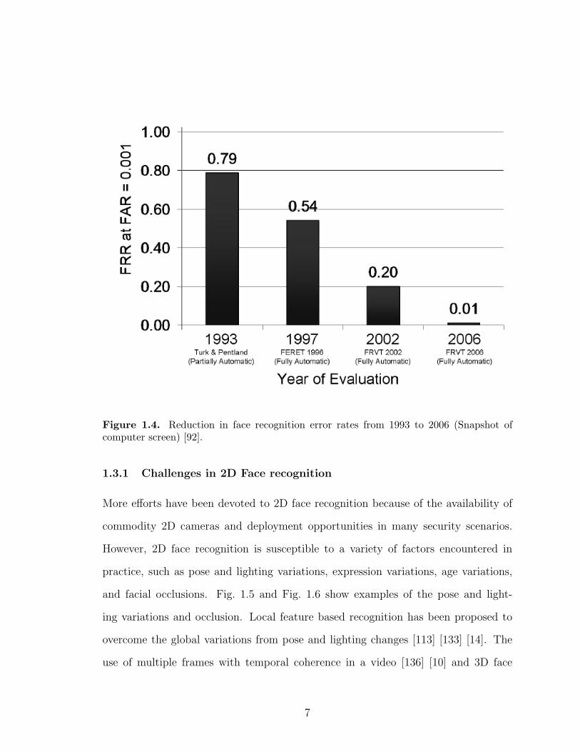
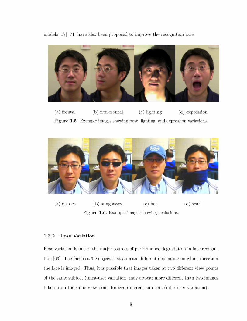


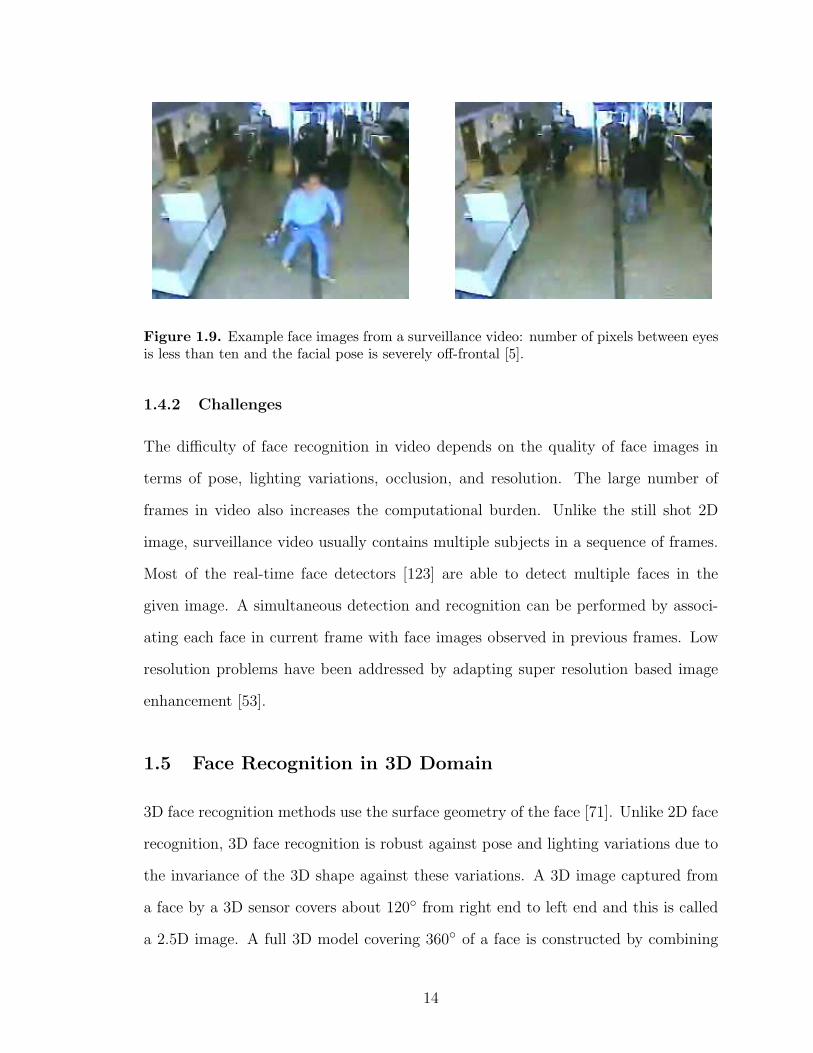

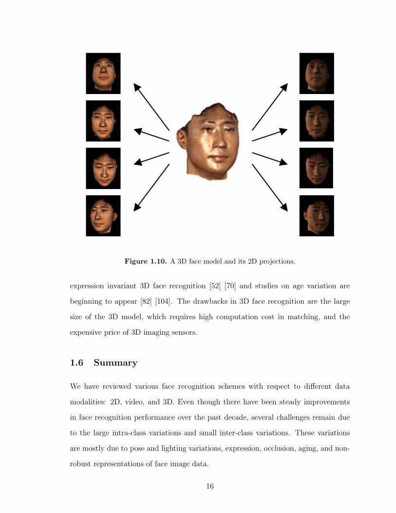


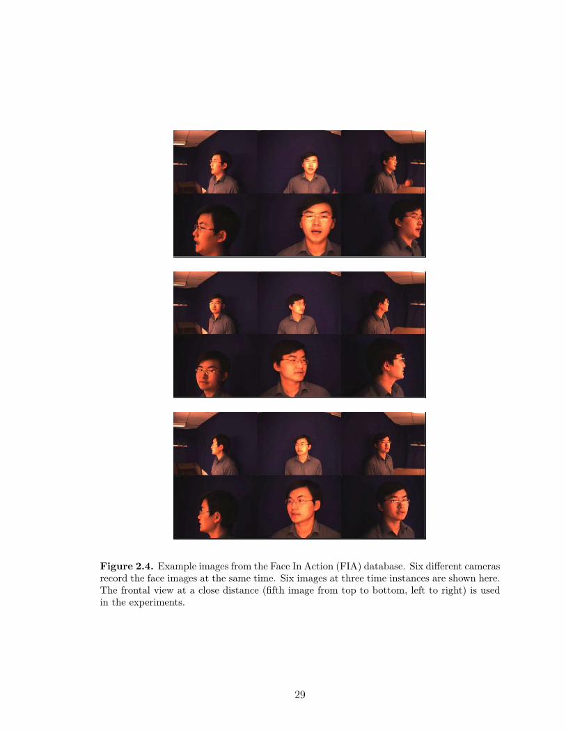
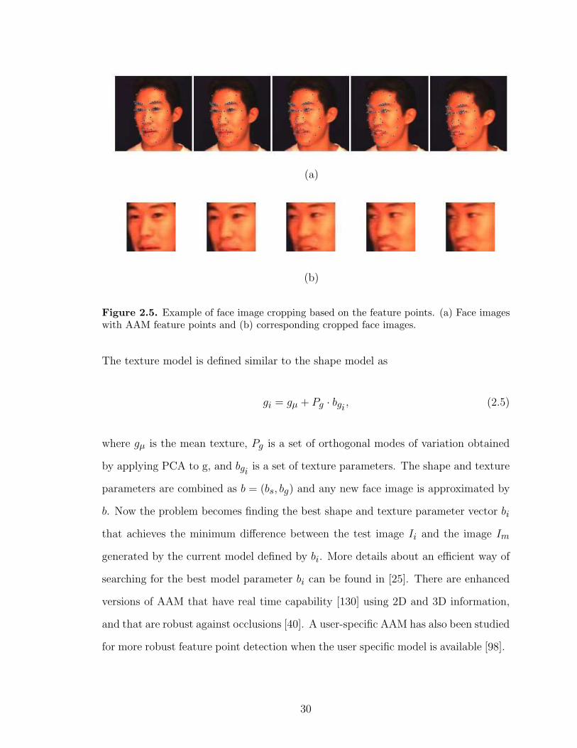


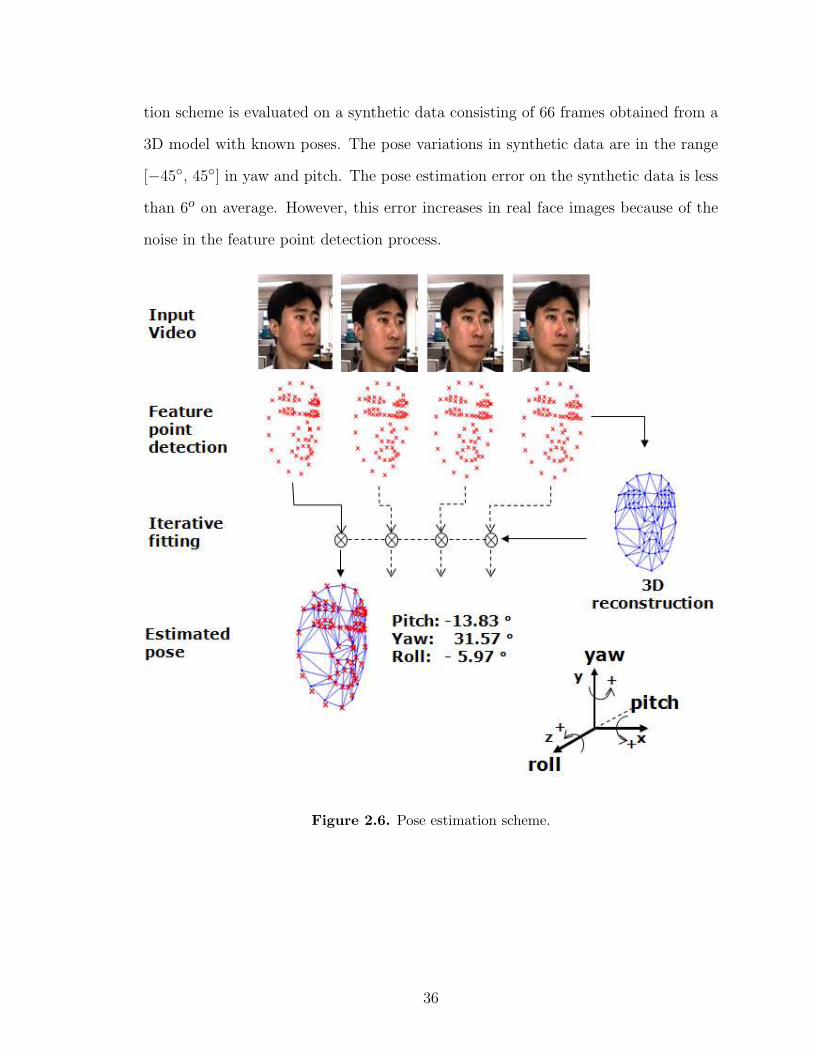


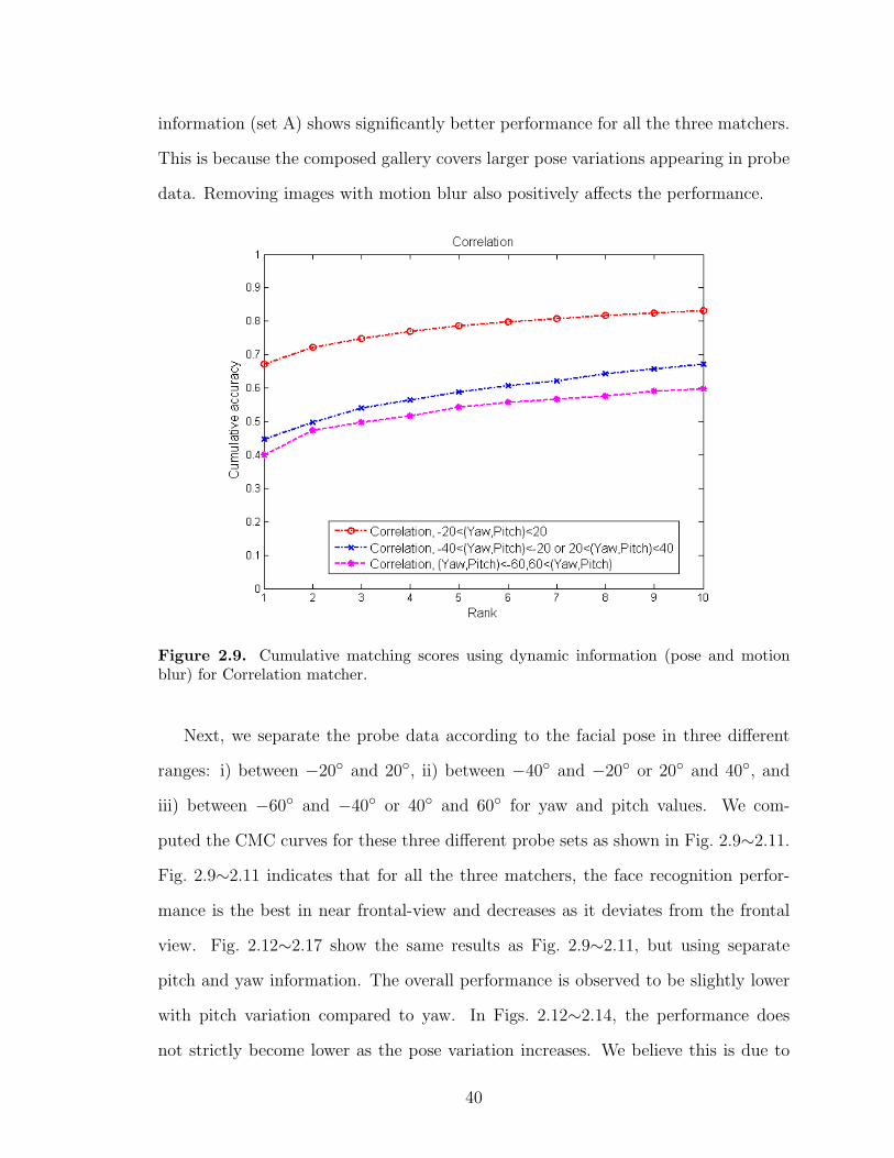


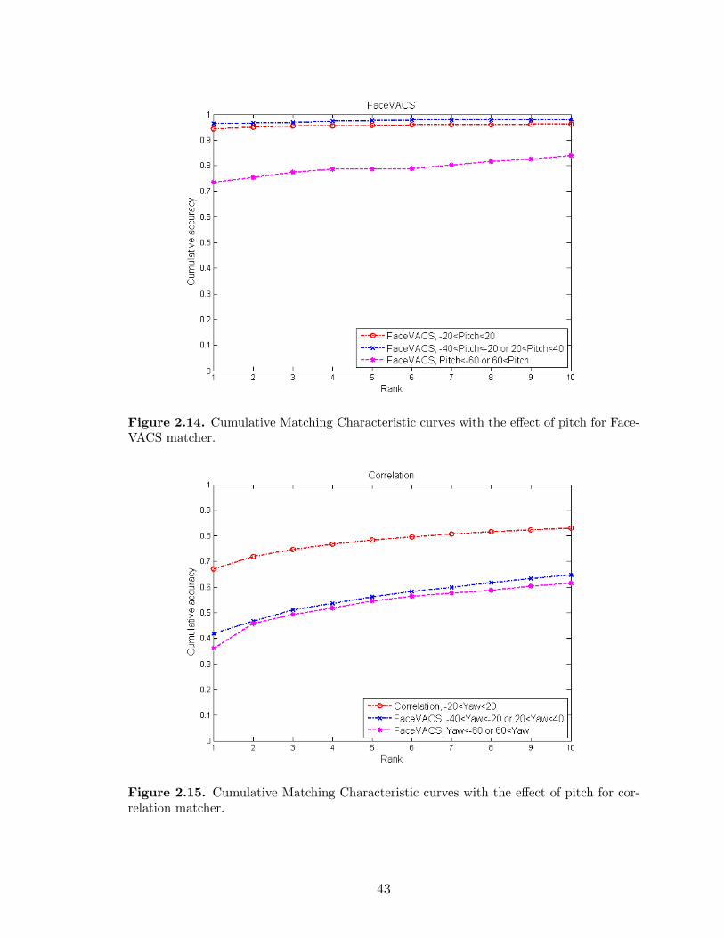

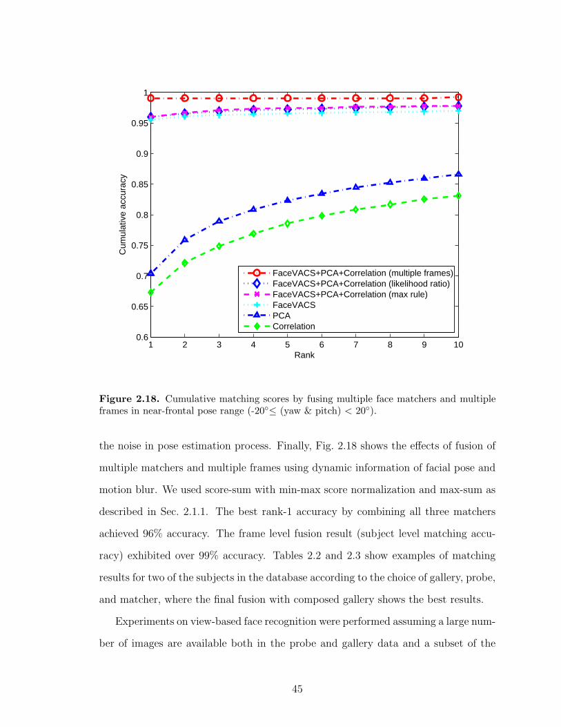
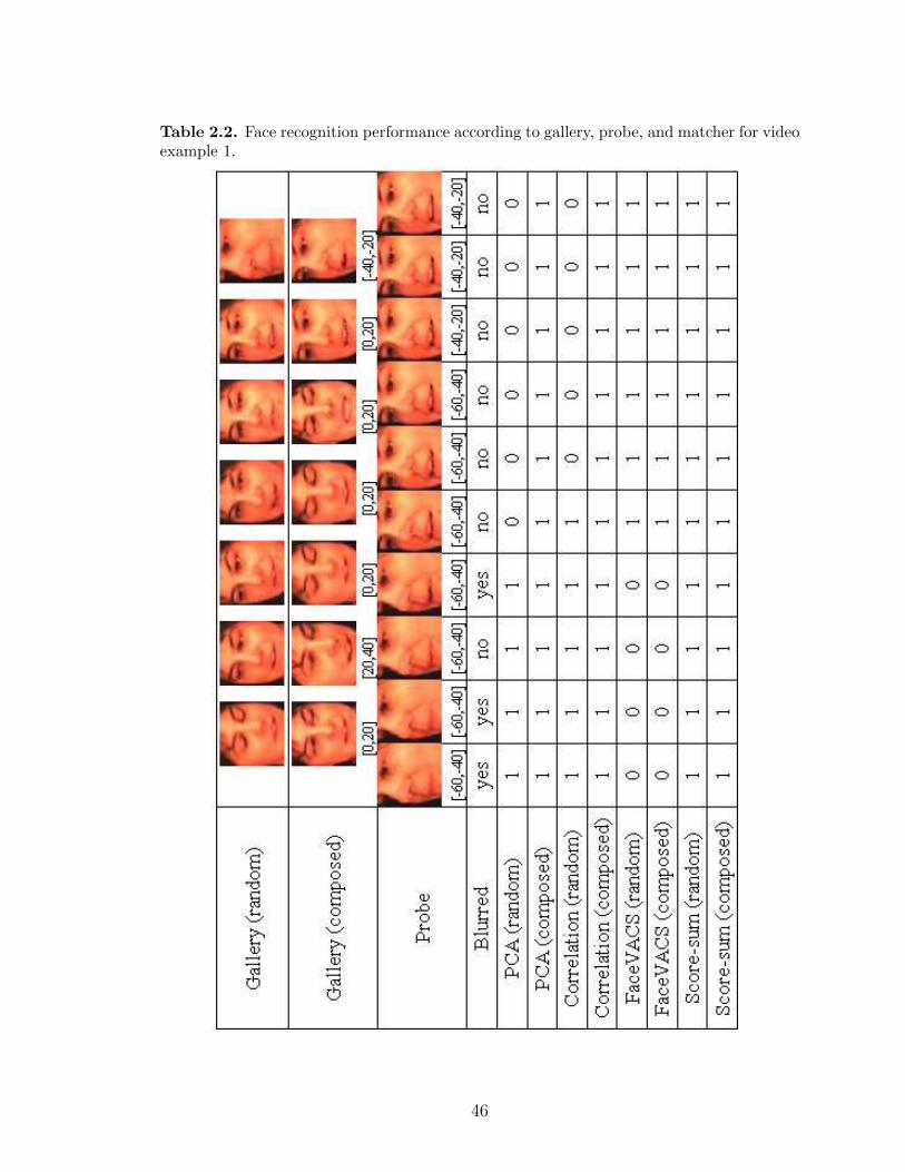

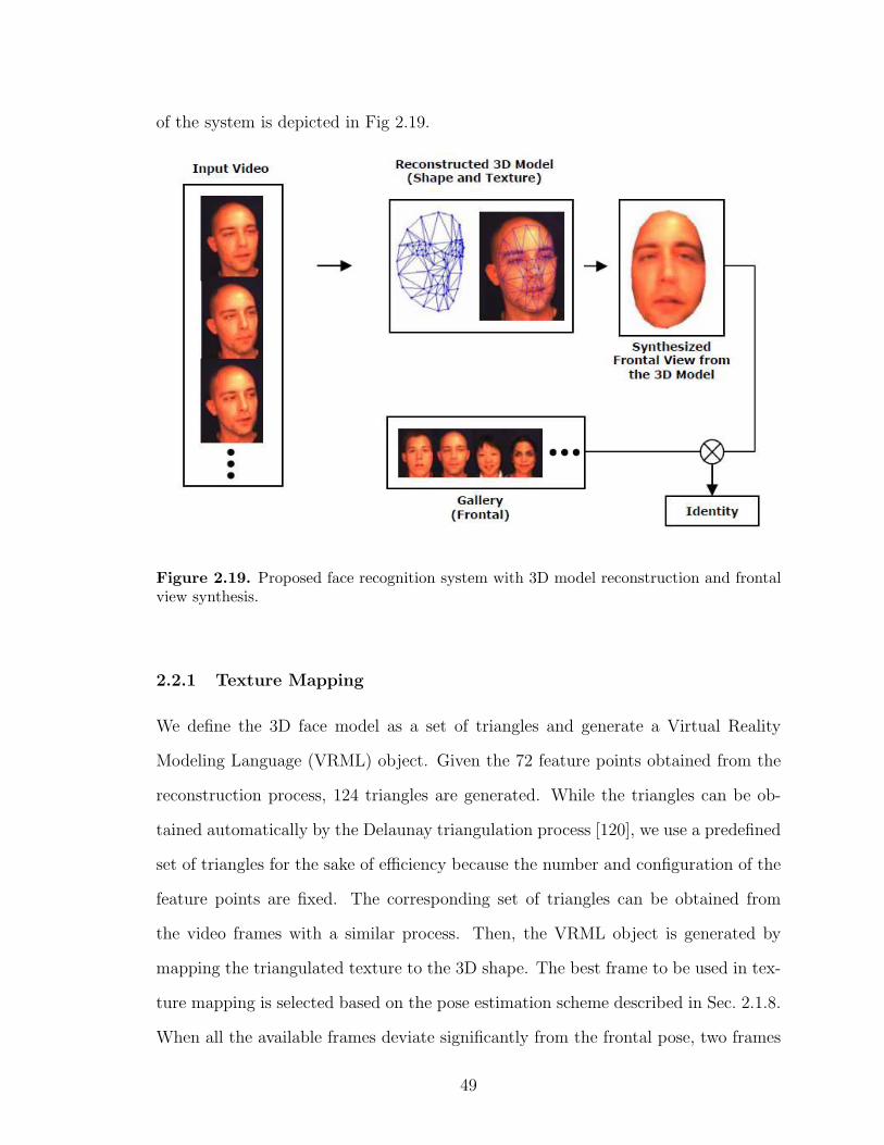
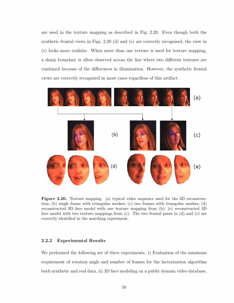

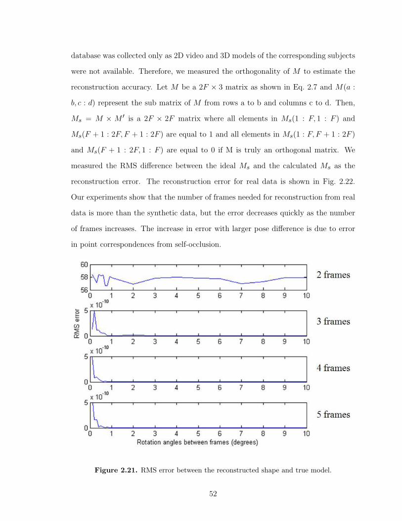

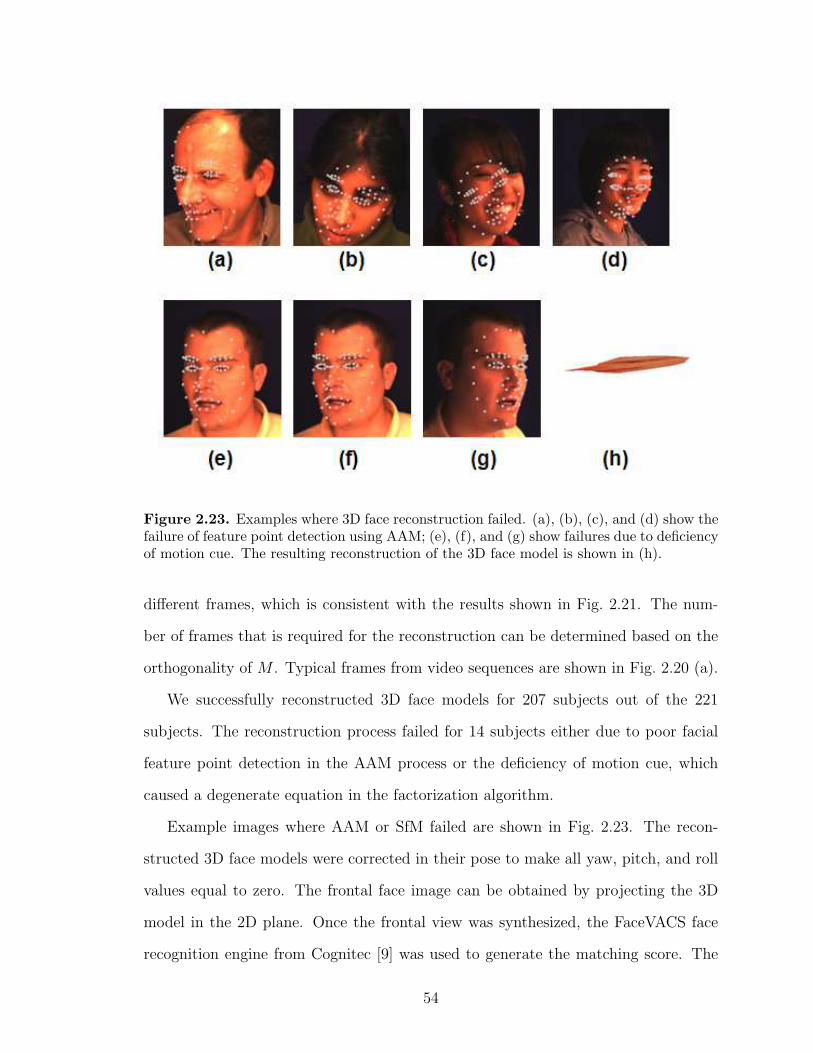

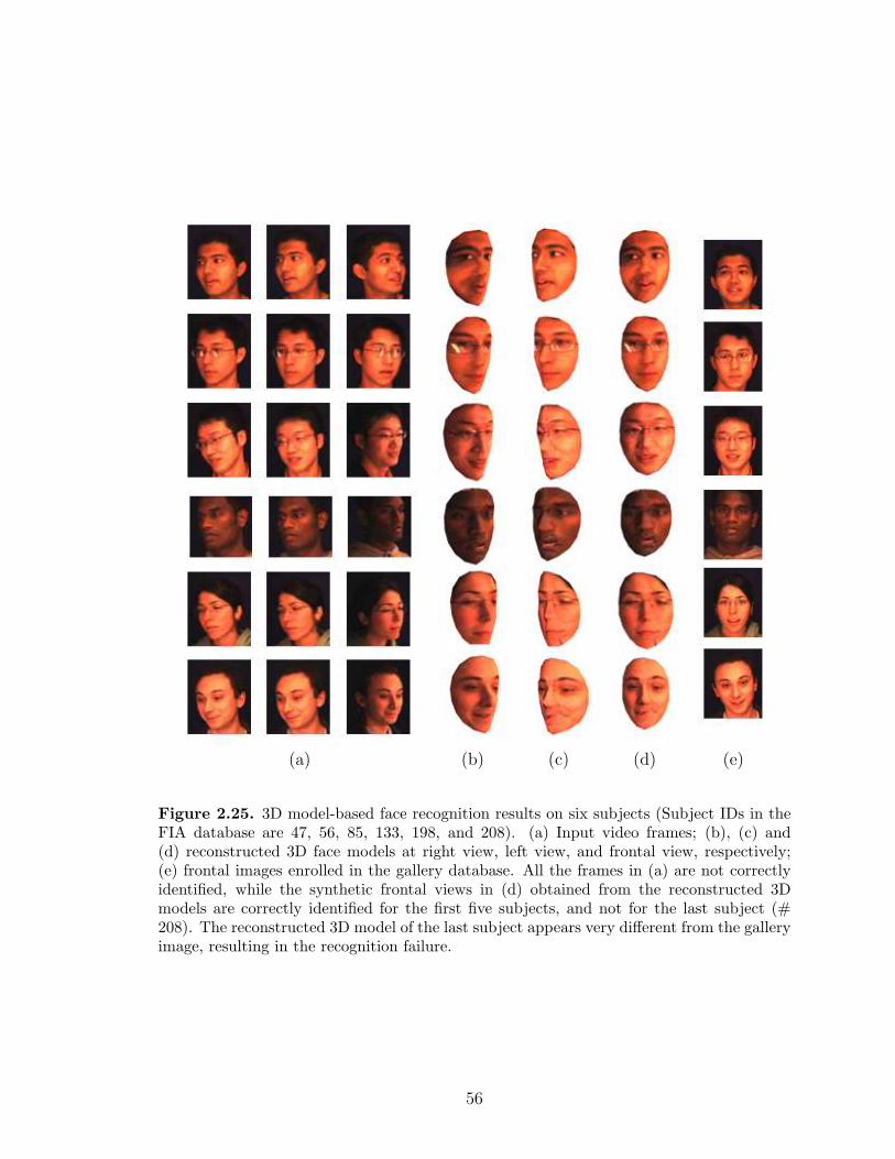
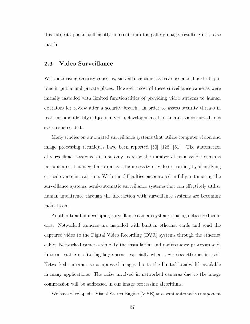


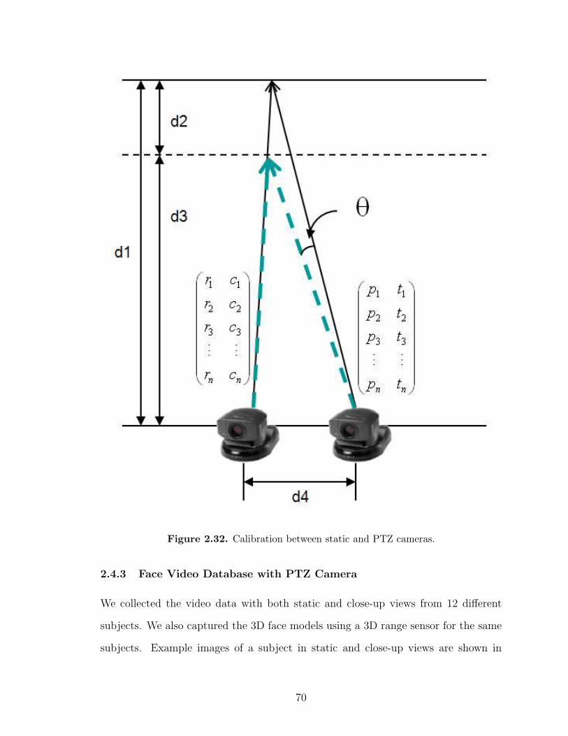
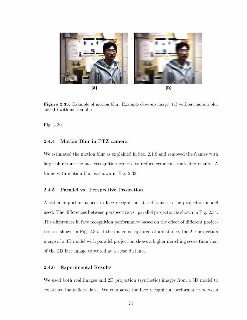
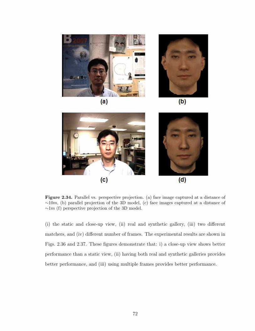
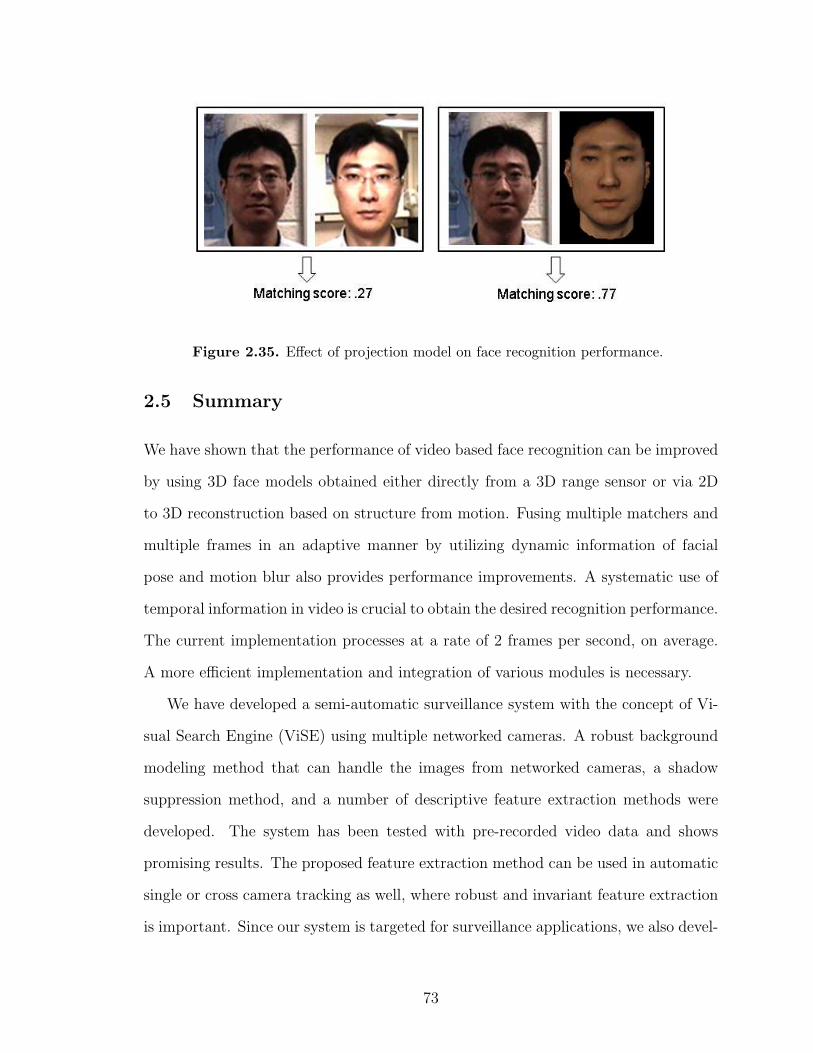
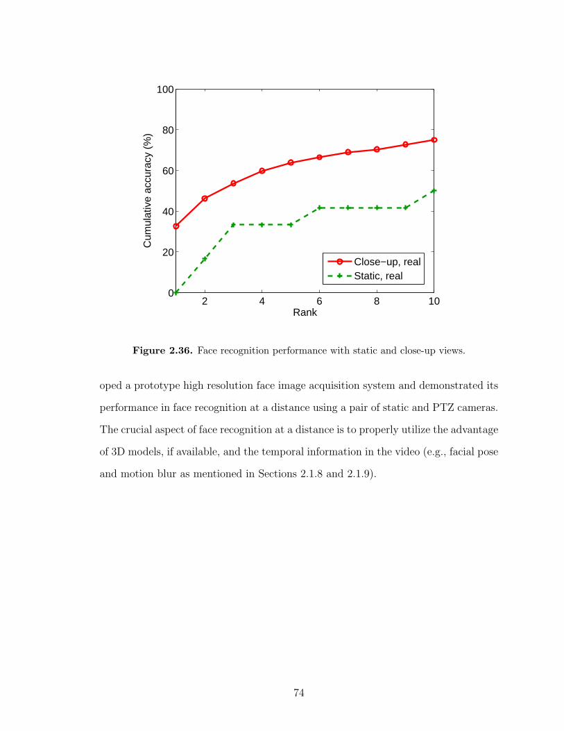
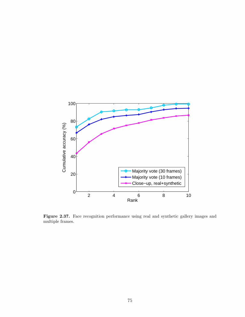


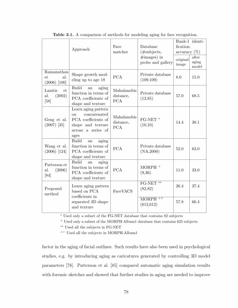


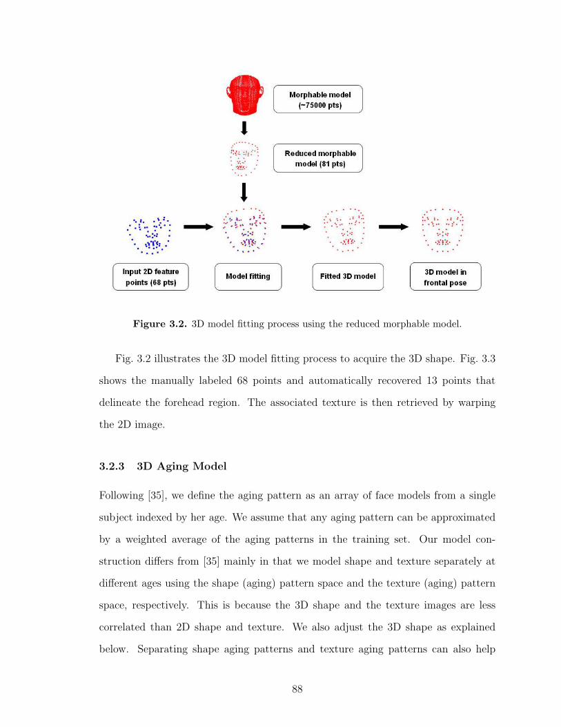
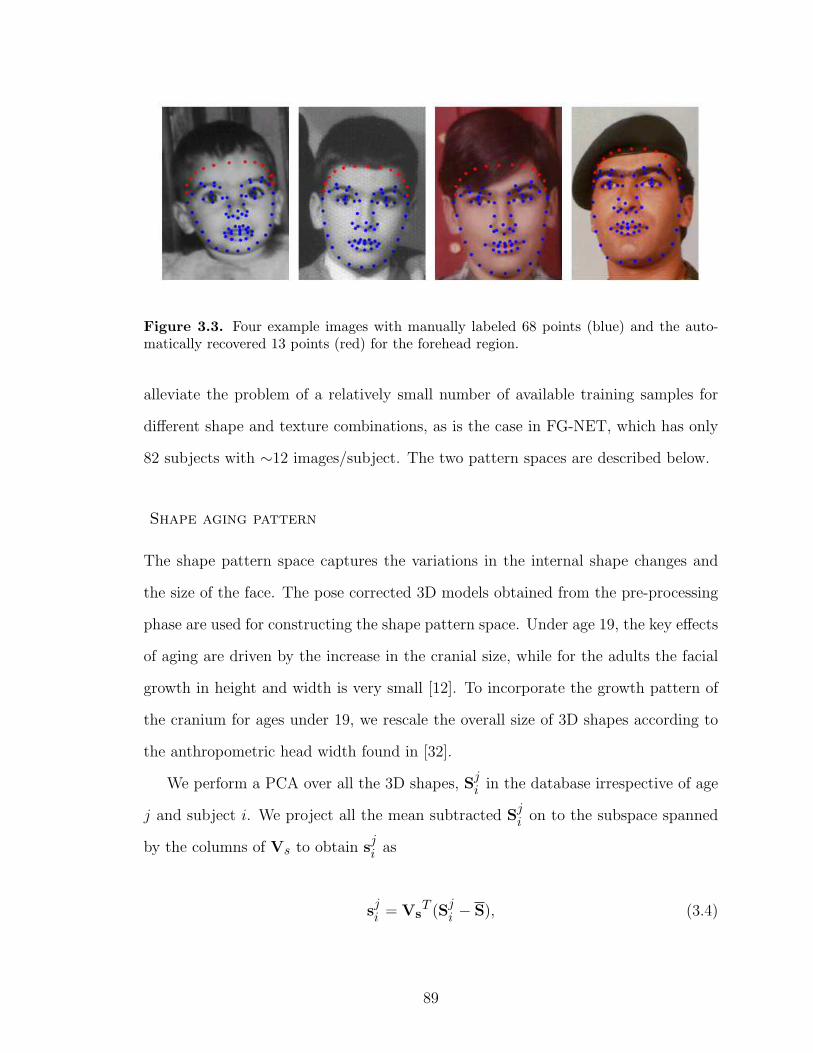
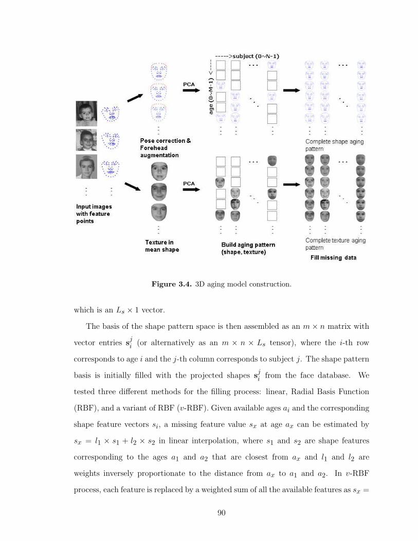


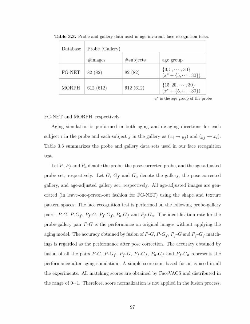

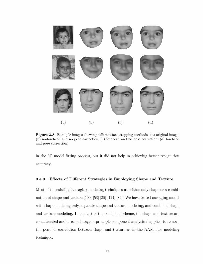
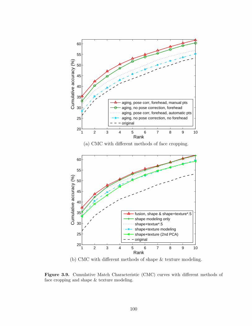


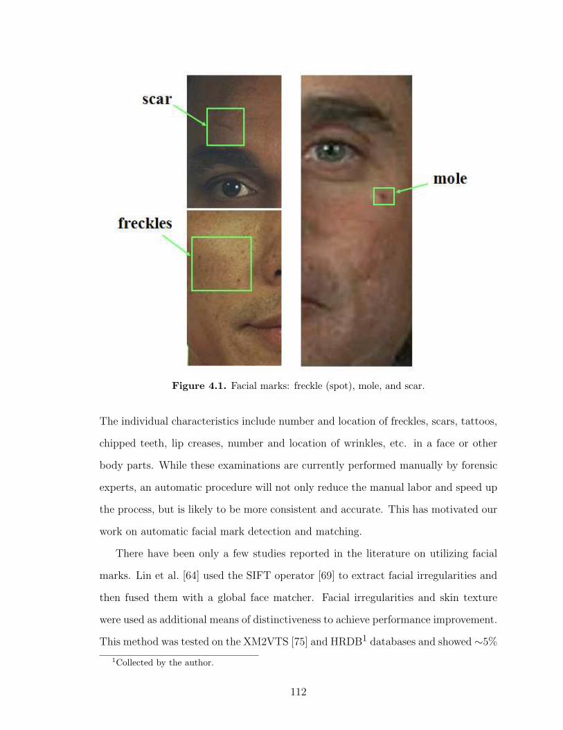

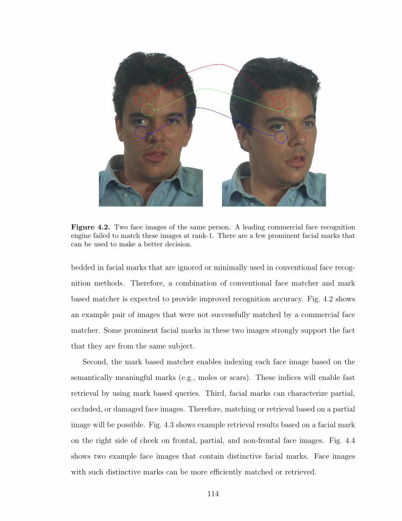


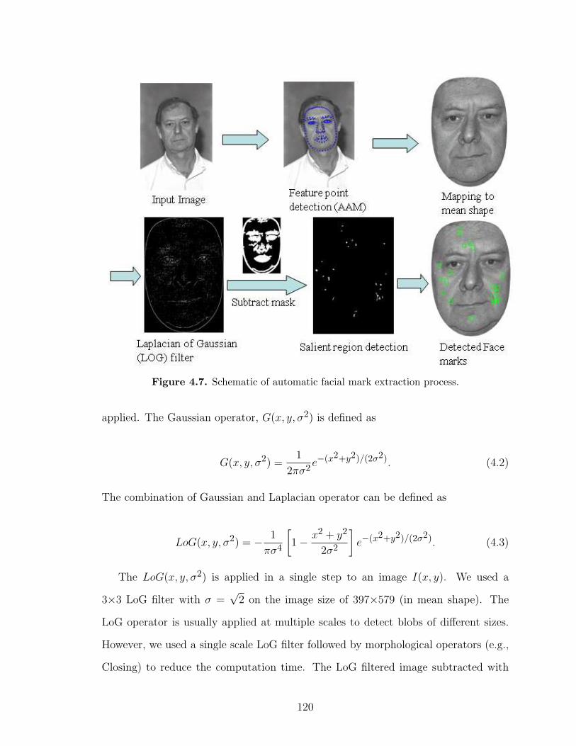


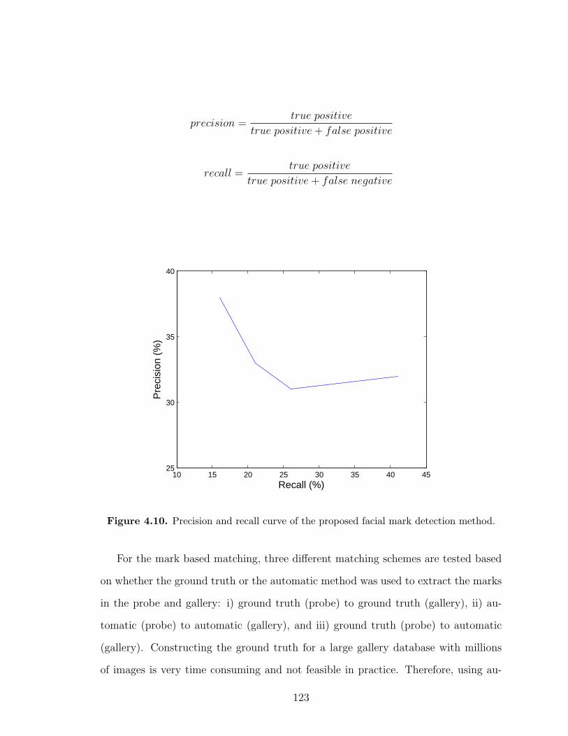

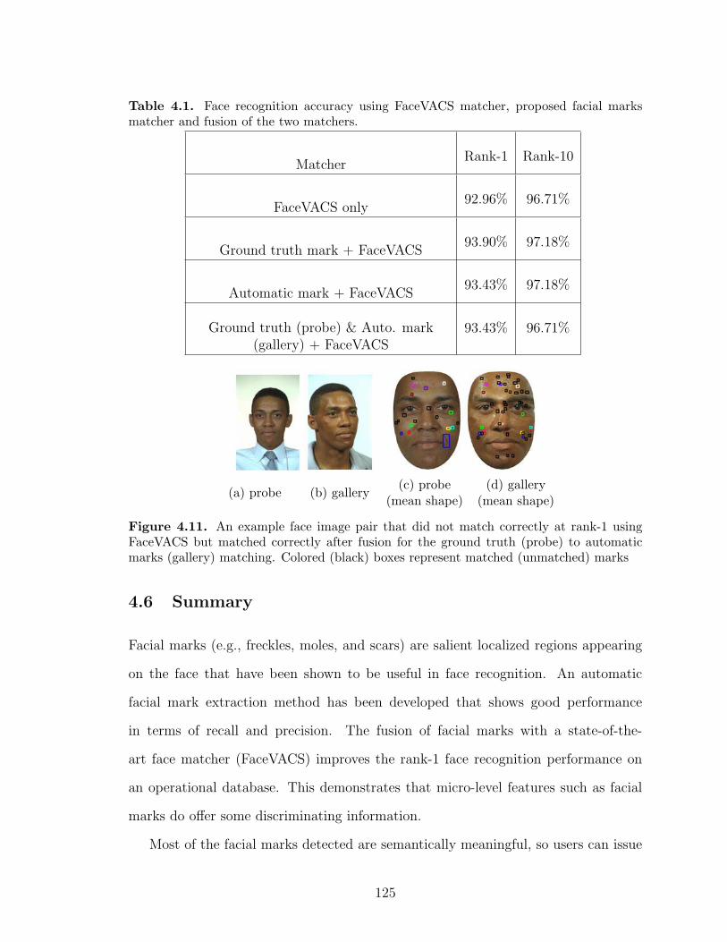


![Low Quality Video Face Recognition: Multi-mode ...biometrics.cse.msu.edu/Publications/Fingerprint/Gongetal...Gong et al. [10] extended the aggregation model by con-sidering component-wise](https://static.documents.pub/doc/80x56/6076b3332cee5006865919bb/low-quality-video-face-recognition-multi-mode-gong-et-al-10-extended.jpg)


![Face Recognition Performance: Role of …biometrics.cse.msu.edu/Publications/Face/Klareetal_Face...demographics considered is intended to augment previous experiments [3], [4] on whether](https://static.documents.pub/doc/80x56/5f0ff7c97e708231d446c83a/face-recognition-performance-role-of-demographics-considered-is-intended-to.jpg)


