87
Nonlinear systems, chaos and control in Engineering Module 1 One-dimensional systems Cristina Masoller [email protected] http://www.fisica.edu.uy/~cris/

Nonlinear systems, chaos
and control in Engineering
Module 1
One-dimensional systems
Cristina Masoller
http://www.fisica.edu.uy/~cris/

Schedule
Flows on the line
(Strogatz ch.1 & 2)
3 hs
Introduction
Fixed points and
linear stability
Solving
equations with
computer
Feedback control
and delays
Bifurcations
(Strogatz ch. 3)
5 hs
Introduction
Saddle-node
Transcritical
Pitchfork
Examples
Flows on the
circle
(Strogatz ch. 4)
2 hs
Introduction to
phase
oscillators
Nonlinear
oscillator
Fireflies and
entrainment

Introduction to dynamical systems
Introduction to flows on the line
Solving equations with computer
Fixed points and linear stability
Feedback control: delay differential equations
Flows on the line: outline

Systems that evolve in time.
Example: a pendulum clock
“Theory of Dynamical Systems”: studies systems that evolve in
time.
They can be linear or nonlinear.
In this course: we focus on nonlinear systems (Nonlinear
Dynamics).
Dynamical systems can be deterministic or stochastic.
Dynamical Systems

An example of a nonlinear dynamical
system: a typical neuron
Koch Nature1997

Stochastic nonlinear dynamics
Koch Nature1997

Possible evolution:
• The system settles down to
equilibrium (rest state or “fixed
point”)
• Keeps repeating in cycles (“limit
cycle”)
• More complicated: chaotic or
complex evolution (“chaotic
attractor”)
Different types of deterministic
dynamical behaviors

Isaac Newton (mid-1600s): ordinary differential
equations.
Planetary orbits: solved analytically the “two-body”
problem (earth around the sun).
Since then: a lot of effort for solving the “three-
body” problem (earth-sun-moon) – Impossible.
Historical development of the
Theory of Dynamical Systems

Patented the first pendulum clock.
Observed the synchronization of two clocks.
Christiaan Huygens (mid-1600s,
Dutch mathematician)

Henri Poincare (French mathematician).
Instead of asking
“which are the exact positions of planets (trajectories)?”
he asked: “is the solar system stable for ever, or will planets
eventually run away?”
He developed a geometrical approach to solve this problem.
Introduced the concept of “phase space”.
He also had an intuition of the possibility of chaos:
“The evolution of a deterministic system can be aperiodic,
unpredictable, and strongly depends on the initial conditions”
Deterministic system: the present state determines future state
(there is no randomness but the system is unpredictable!)
Late 1800s

Computers drove economic growth and transformed
how we live and work.
They also allowed to experiment with equations.
Powerful tool to advance the “Theory of Dynamical
Systems”.
1960s: Eduard Lorentz (American mathematician
and meteorologist at MIT): simple model of
convection rolls in the atmosphere.
Glimpse (intuition) of chaotic motion on a strange
attractor.
He also showed that there is structure and order in
chaotic motion.
First simulations (1950s)

Lorentz studied meteorological prediction using
Navier-Stokes simplified equations:
The Lorentz system
bzxyz
yzrxy
yxx
)(
)(
3 variables:
x: rotation rate of a cylindrical mass of gas,
y: thermal gradient,
z: temperature variation.
3 Parameters:
: Prandtl number (ratio between viscosity and thermal conductivity),
R: Rayleigh number (temperature difference between top and bottom of
cylinder),
b: ratio between width and height of the cylinder.

Starting from an initial condition (x0, y0, z0) by
numerically integrating the equations we can plot the
trajectory in the phase space (Lorentz’s Attractor).
Lorentz’s Attractor
Lorentz found
extreme
sensitive to
initial conditions
impossibility
of long-term
meteorological
predictions.

Ilya Prigogine (Belgium, born in Moscow, Nobel
Prize in Chemistry 1977)
Thermodynamic systems far from equilibrium.
Discovered that, in chemical systems, the interplay
of (external) input of energy and dissipation can
reverse the rule of maximization of entropy (second
law of thermodynamics).
Order within chaos and
self-organization
Introduced the concepts of “self-organization” and
“dissipative structures”.
Wide implications to biological systems and the evolution of
life.

H = 0
C = 0
H = Max
C = 0
H ≠ 0
C ≠ 0

Newtonian physics has been extended three times:
• First, with the use of the wave function in quantum
mechanics.
• Then, with the introduction of space-time in relativity.
• And finally, with the recognition of indeterminism in
nonlinear systems.
Chaos is the third great revolution of 20th-century
physics, after relativity and quantum theory.
According to Prigogine

Robert May (Australian): population biology
"Simple mathematical models with very complicated
dynamics“, Nature (1976).
The 1970s
• Difference equations (“iterated maps”) arise in many contexts in the
biological, economic and social sciences.
• Such equations, even though simple and deterministic, can exhibit a
surprising array of dynamical behavior, from stable points, to a
bifurcating hierarchy of stable cycles, to apparently random
fluctuations.
• There are consequently many fascinating problems, some concerned
with delicate mathematical aspects of the fine structure of the
trajectories, and some concerned with the practical implications and
applications.
xt+1 = f (xt)

Models of dynamical systems
Continuous-time
differential equations
bzxyz
yzrxy
yxx
)(
)( )1( 1 ttt xxrx
),( rxfxdt
dx ),(1 rxfx tt
r = control parameter(s)
Example: Lorentz model Example: Logistic “map”
Difference equations
(iterated maps)

The logistic map
0 10 20 30 40 500
0.5
1 r=3.5
i
x(i
)
0 10 20 30 40 500
0.5
1r=3.3
i
x(i
)
0 10 20 30 40 500
0.5
1
r=3.9
i
x(i
)
0 10 20 30 40 500
0.5
1r=2.8
i
x(i
)
Sequence of “period-doubling”
bifurcations to chaotic behavior
)1( 1 iii xxrx
Parameter r
x(i)

In 1975, Mitchell Feigenbaum (American
mathematical physicist), using a small HP-
65 calculator, discovered that
Universal route to chaos
...6692.4lim1
21
nn
nnn
rr
rr
Then, he provided a mathematical proof (by using the
“renormalization concept” –connecting to phase transitions in
statistical physics).
Then, he showed that the same behavior, with the same
mathematical constant, occurs within a wide class of functions,
prior to the onset of chaos (universality).
Very different systems (in chemistry, biology, physics,
etc.) go to chaos in the same way, quantitatively.

The first magnetic card-programmable handheld
calculator
HP-65 calculator
HP-65 in original hard
case with manuals,
software "Standard
Pac" of magnetic
cards, soft leather
case, and charger

Benoit Mandelbrot (Polish-born, French
and American mathematician 1924-
2010): “self-similarity” and fractal
objects:
each part of the object is like the whole
object but smaller.
Because of his access to IBM's
computers, Mandelbrot was one of the
first to use computer graphics to create
and display fractal geometric images.
The late 1970s

Are characterized by a “fractal” dimension that measures
roughness (more in Module 3)
Fractal objects
Video: http://www.ted.com/talks/benoit_mandelbrot_fractals_the_art_of_roughness#t-149180
Romanesco broccoli
D=2.66
Human lung
D=2.97 Coastline of Ireland
D=1.22

Arthur Winfee (American theoretical biologist –
born in St. Petersburg): Large communities of
nonlinear biological oscillators show a tendency
to self-organize in time –collective
synchronization.
Biological nonlinear oscillators
In the 1960’s he did experiments trying to understand the
effects of perturbations in biological clocks (circadian rhythms).
What is the effect of an external perturbation on
subsequent oscillations?

He studied the periodic emergence of a fruit fly that as a 24-
hour rhythmic emergency.
Using brief pulses of light, found that the periodic emergence of
the flies was shifted, and the shift depended on the timing and
the duration of the light pulse.
Also found that there is a critical timing and duration that results
in no further periodic emergency (destroys the biological clock).
The work has wide implications, for example, for cardiac tissue:
some cardiac failures are related to perturbed oscillators.
Winfee work on perturbing
biological oscillators

Synchronization

Model of coupled phase oscillators.
K = coupling strength, i = stochastic term (noise)
Describes the emergence of collective behavior (synchronization)
How to quantify synchronization?
With the order parameter:
NiN
K
dt
di
N
j
ijii ...1 ,)sin(
1
N
j
ii jeN
re1
1
Kuramoto model
(Japanese physicist, 1975)
r =0 incoherent state (oscillators are scattered in the unit circle)
r =1 all oscillators are in phase (i=j i,j)

Synchronization transition as the
coupling strength increases
Strogatz
Nature 2001
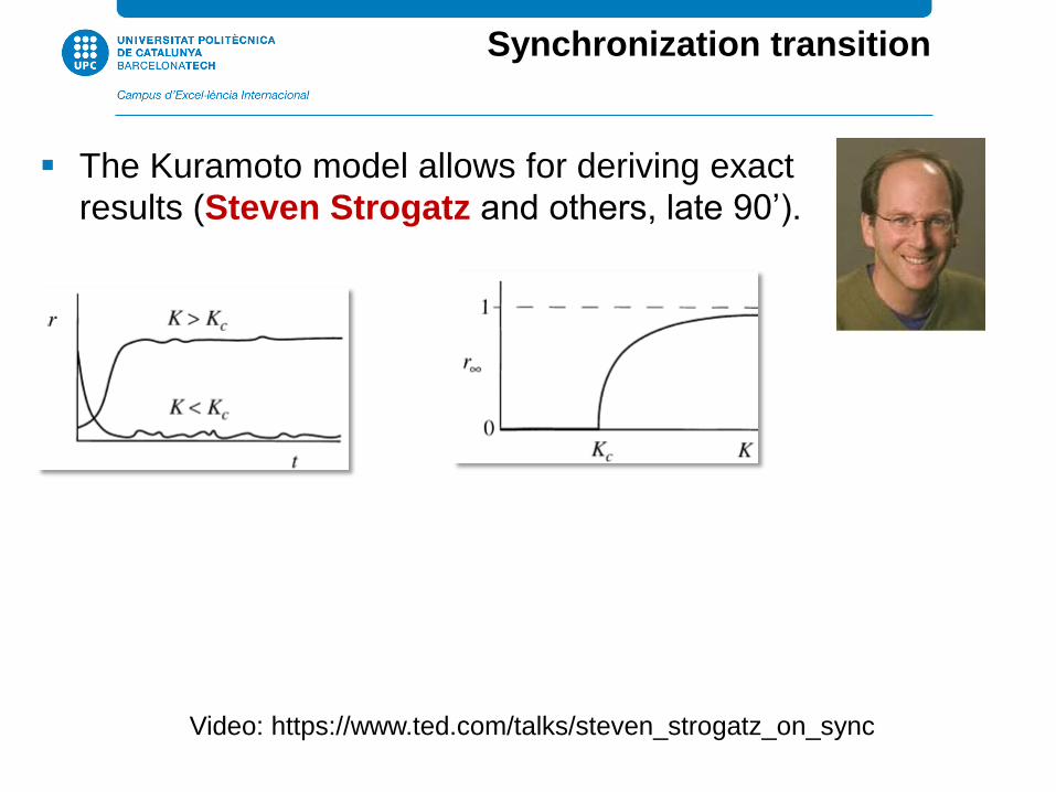
The Kuramoto model allows for deriving exact
results (Steven Strogatz and others, late 90’).
Synchronization transition
Video: https://www.ted.com/talks/steven_strogatz_on_sync

Optical chaos: first observed in laser systems.
In the 80’s: can we observe
chaos experimentally?
Time
…
…
Interested? visit our lab!

Ott, Grebogi and Yorke (1990)
Unstable periodic orbits can be used for control: wisely
chosen periodic kicks can maintain the system near the
desired orbit.
Pyragas (1992)
Control by using a continuous self-controlling feedback
signal, whose intensity is practically zero when the system
evolves close to the desired periodic orbit but increases
when it drifts away.
In the 90’: can we control
chaotic dynamics?

Raj Roy and others (1994)
Experimental demonstration of
control of optical chaos

33
I. Kanter et al, Nature Photonics 2010
After processing the signal, arbitrarily long sequences
can be generated at the 12.5-Gbit/s rate.
In the last decade: can we
exploit / use chaotic dynamics?
An example from optical chaos: ultra-fast generation of random bits

Laser spikes: intensity vs. time
Optical dynamical systems:
a few examples from our lab
Neuronal spikes
Extreme pulses

Interest moves from chaotic systems to complex systems
(low vs. very large number of variables).
Networks (or graphs)!
End of 90’s and 2000-present
Strogatz
Nature 2001

Take home message
Dynamical complex systems have multiple applications,
and involve the work of mathematicians, physicists,
biologists, computer scientists, engineers, etc.
Interested? TFGs available, contact us.

Introduction to dynamical systems
Introduction to flows on the line
Solving equations with computer
Fixed points and linear stability
Feedback control: delay differential equations
Outline
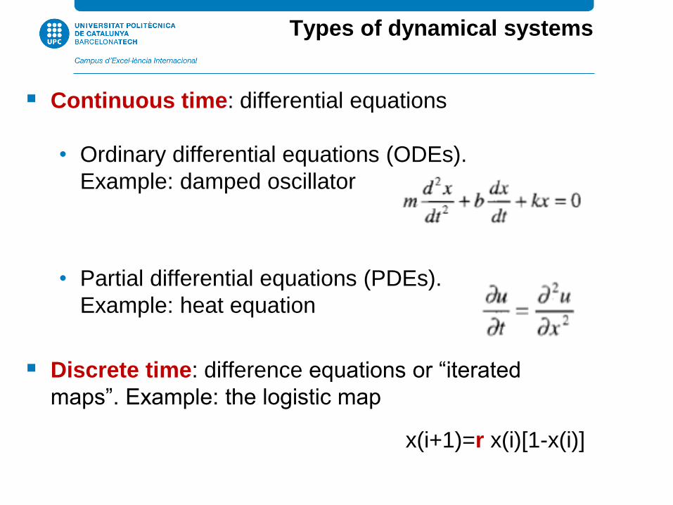
Continuous time: differential equations
• Ordinary differential equations (ODEs).
Example: damped oscillator
• Partial differential equations (PDEs).
Example: heat equation
Discrete time: difference equations or “iterated
maps”. Example: the logistic map
Types of dynamical systems
x(i+1)=r x(i)[1-x(i)]

ODEs can be written as first-
order differential equations
First example: harmonic oscillator
Second example: pendulum
)(xfx

Trajectory in the phase space
Given the initial conditions, x1(0) and x2(0),
we predict the evolution of the system by
solving the equations: x1(t) and x2(t).
x1(t) and x2(t) are solutions of the equations.
The evolution of
the system can be
represented as a
trajectory in the
phase space.
two-dimensional
(2D) dynamical
system. Key argument (Poincare): find out
how the trajectories look like, without
solving the equations explicitly.

f(x) linear: in the function f, x appears to first order only
(no x2, x1x2, sin(x) etc.). Then, the behavior can be
understood from the sum of its parts.
f(x) nonlinear: superposition principle fails!
Classification of dynamical systems
described by ODEs (I/II)
)()( txfx
Example of linear system: harmonic oscillator
In the right-hand-side x1
and x2 appear to first
power (no products etc.)
Example of nonlinear system: pendulum

Classification of dynamical systems
described by ODEs (II/II)
)()( txfx
=0: deterministic.
0: stochastic (real life) –simplest case: additive noise.
x: vector with few variables (n<4): low dimensional.
x: vector with many variables: high dimensional.
f does not depend on time: autonomous system.
f depends on time: non-autonomous system.

3D system: to predict the future evolution we
need to know the present state (t, x, dx/dt).
Example of non-autonomous
system: a forced oscillator
Can also be written as first-order ODE

Harmonic
oscillator
Pendulum
• Heat
equation,
• Maxwell
equations
• Schrodinger
equation
RC circuit
Logistic
population
grow
• Navier-
Stokes
(turbulence)
N=1 N=2 N=3 N>>1 N= (PDEs)
Linear
Nonlinear • Forced
oscillator
• Lorentz
model
• Kuramoto
phase
oscillators
• Networks
Summary
Number of variables

One-dimensional dynamical system
(first-order ordinary differential equation)
x
f does not depend on time (if it does, it is a non-
autonomous system = second-order ODE).
What is a “flow on the line”?

Introduction to dynamical systems
Introduction to flows on the line
Solving equations with computer
Fixed points and linear stability
Feedback control: delay differential equations
Outline

Euler method
Numerical integration
Euler second order

Fourth order (Runge-Kutta 1905)
Problem if t is too small: round-off errors
(computers have finite accuracy).


Example 1
0 2 4 6 8 100
0.2
0.4
0.6
0.8
1
1.2
1.4
1.6
1.8
2
ty(t
)
%vector_field.m
n=15;
tpts = linspace(0,10,n);
ypts = linspace(0,2,n);
[t,y] = meshgrid(tpts,ypts);
pt = ones(size(y));
py = y.*(1-y);
quiver(t,y,pt,py,1);
xlim([0 10]), ylim([0 2])
• quiver(x,y,u,v,scale): plots
arrows with components (u,v)
at the location (x,y).
• The length of the arrows is
scale times the norm of the
(u,v) vector.
)1( yyy
To plot the blue arrows:

Numerical solution
0 2 4 6 8 100
0.2
0.4
0.6
0.8
1
1.2
1.4
1.6
1.8
2
ty(t
)
tspan = [0 10];
yzero = 0.1;
[t, y] =ode45(@myf,tspan,yzero);
plot(t,y,'r*--'); xlabel t; ylabel y(t)
)1( yyy 1.0)0( y
function yprime = myf(t,y)
yprime = y.*(1-y);
To plot the solution (in red):
The solution is always tangent to the arrows
Remember: HOLD to plot together the blue
arrows & the trajectory.

Example 2
0 0.5 1 1.5 2 2.5 3-1.5
-1
-0.5
0
0.5
1
1.5
t
y(t
)
n=15;
tpts = linspace(0,3,n);
ypts = linspace(-1.5,1.5,n);
[t,y] = meshgrid(tpts,ypts);
pt = ones(size(y));
py = -y-5*exp(-t).*sin(5*t);
quiver(t,y,pt,py,1);
xlim ([0 3.2]), ylim([-1.5 1.5])
function yprime = myf(t,y)
yprime = -y -5*exp(-t)*sin(5*t);
tspan = [0 3];
yzero = -0.5;
[t, y] = ode45(@myf,tspan,yzero);
plot(t,y,'kv--'); xlabel t; ylabel y(t)
teyy t 5sin5 5.0)0( y

General form of a call to Ode45

Introduction to dynamical systems
Introduction to flows on the line
Solving equations with computer
Fixed points and linear stability
Feedback control: delay differential equations
Outline

Example
Starting from x0=/4, what is the long-term behavior (what
happens when t?)
And for any arbitrary condition xo?
We look at the “phase portrait”: geometrically, picture of all
possible trajectories (without solving the ODE analytically).
Imagine: x is the position of an imaginary particle restricted to
move in the line, and dx/dt is its velocity.
Analytical Solution:

Imaginary particle moving in the
horizontal axis
x0 =/4
x0 arbitrary
Flow to the right when
Flow to the left when 0x
0x
0x “Fixed points”
Two types of FPs: stable & unstable

Fixed points
Fixed points = equilibrium solutions
Stable (attractor or sink): nearby
trajectories are attracted
and -
Unstable: nearby trajectories are
repelled
0 and 2

Find the fixed points and classify their stability
Example 1

Example 2

N(t): size of the population of the species at time t
Example 3: population model for
single species (e.g., bacteria)
Simplest model (Thomas Malthus 1798): no migration,
births and deaths are proportional to the size of the
population
Exponential grow!

More realistic model:
logistic equation
If N>K the population decreases
If N<K the population increases
To account for limited food (Verhulst 1838):
The carrying capacity of a biological species in an
environment is the maximum population size of the species
that the environment can sustain indefinitely, given the food,
habitat, water, etc.
K = “carrying capacity”

How does a population approach
the carrying capacity?
Good model only for simple
organisms that live in constant
environments.
Exponential or sigmoid approach.

And the human population?
Source: wikipedia
Hyperbolic grow !
Technological advance
→ increase in the carrying
capacity of land for people
→ demographic growth
→ more people
→ more potential inventors
→ acceleration of
technological advance
→ accelerating growth of
the carrying capacity…

the perturbation grows exponentially
Linearization close to a
fixed point
the perturbation decays exponentially
Second-order terms can not be neglected and a
nonlinear stability analysis is needed.
Bifurcation (more latter)
Characteristic time-scale
The slope f’(x*) at the fixed point determines the stability
= tiny perturbation
Taylor expansion

Existence and uniqueness
Problem: f ’(0) infinite
When the solution of dx/dt = f(x) with x(0) = x0 exists and is
unique?
Short answer: if f(x) is “well behaved”, then a solution exists
and is unique.
“well behaved”?
f(x) and f ’(x) are both continuous on an interval of x-values
and that x0 is a point in the interval.
Details: see Strogartz section 2.3.

Linear stability of the fixed points of
Example 1
Stable: and -
Unstable: 0, 2
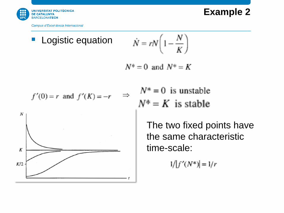
Logistic equation
Example 2
The two fixed points have
the same characteristic
time-scale:

Good agreement with controlled
population experiments

Lack of oscillations
General observation: only
sigmoidal or exponential
behavior, the approach is
monotonic, no oscillations
Strong damping
(over damped limit)
Analogy:
To observe oscillations we need
to keep the second derivative (weak damping).

Stability of the fixed point x*
when f ’(x*)=0?
In all these systems:
When f’(x*) = 0
nothing can be
concluded
from the
linearization
but these plots
allow to see
what goes on.

Potentials
V(t) decreases along the trajectory.
Example:
Two fixed points: x=1 and x=-1
(Bistability).

Flows on the line = first-order ordinary differential
equations.
dx/dt = f(x)
Fixed point solutions: f(x*) =0
• stable if f´(x*) <0
• unstable if f´(x*) >0
• neutral (bifurcation point) if f´(x*) = 0
There are no periodic solutions; the approach to a fixed
point is monotonic (sigmoidal or exponential).
Summary

Introduction to dynamical systems
Introduction to flows on the line
Solving equations with computer
Fixed points and linear stability
Feedback control: delay differential
equations
Outline

Any system involving a feedback control will almost
certainly involve time delays.
In a 2D system delayed feedback can reduce oscillations,
but in a 1D system it can induce oscillations.
Example:
Exception to no oscillations:
delay differential equations (DDEs)
Linear system
Infinite-dimensional system
Delay-induced oscillations.

Example: population dynamics
Delayed logistic equation
In a single-species population, the incorporation of a delay allows to
explain the oscillations, without the predatory interaction of other species.
The initial function is y=0.5 in -1<s<0

It is important for the crane to move payloads rapidly and
smoothly. If the gantry moves too fast the payload may start
to sway, and it is possible for the crane operator to lose
control of the payload.
Example: Container crane
Delayed feedback control

weakly damped oscillator
Pendulum model for the crane,
y represents the angle
Feedback control
Reduction of payload oscillations: why delayed feedback works?
Near the equilibrium solution y=0:
Small delay:
The delay increases the damping.
Therefore: the oscillations decay faster.
(not first-order equation,
without control payload
oscillations are possible)

Small perturbation
but
Large perturbation

Example: Car following model

Typical solution for two cars
Speed of the two cars Distance between the two cars
The lead vehicle reduces its speed of 80 km/h to 60
km/h and then accelerates back to its original
speed. The initial spacing between vehicles is 10 m.

Alcohol effect
A sober driver needs about 1 s in order to start
breaking in view of an obstacle.
With 0.5 g/l alcohol in blood (2 glasses of wine), this
reaction time is estimated to be about 1.5 s.
oscillations near the stable equilibrium increase.

Solving DDEs
function solve_delay1
tau = 1;
ic = [0.5];
tspan = [0 100];
h = 1.8;
sol = dde23(@f,tau,ic,tspan);
plot(sol.x,sol.y(1,:),'r-')
function v=f(t,y,Z)
v = [h*y(1).*(1-Z(1))];
end
end
0 20 40 60 80 1000
0.5
1
1.5
2
2.5
Example 1: Delayed logistic equation
ic =constant
initial
function

Solving DDEs
0 50 100 150 200 2500
5
10
15
20
25
30
35
40
45
function solve_delay2
tau=9;
ic = [35;10];
tspan = [0 250];
h = 10;
sol = dde23(@f,tau,ic,tspan);
plot(sol.x,sol.y(1,:),'r-',sol.x,sol.y(2,:),'b--')
function v=f(t,y,Z)
v = [y(1)*(2*(1-y(1)/50)-y(2)/(y(1)+40))-h
y(2)*(-3+6*Z(1)/(Z(1)+40))];
end
end
Example 2: Prey (x) and predator (y) model

Class and homework
10-4
10-2
100
10-15
10-10
10-5
100

0 2 4 6 8 10-1
0
1
2
3
4
5
6
7
8
9
10
)0(21
)0()(
2tx
xtx

Steven H. Strogatz: Nonlinear dynamics
and chaos, with applications to physics,
biology, chemistry and engineering
(Addison-Wesley Pub. Co., 1994).
Chapters 1 and 2
Thomas Erneux: Applied delay differential
equations (Springer 2009).
D. J. Higham and N. J. Higham, Matlab
Guide Second Edition (SIAM 2005)
Bibliography


