Process Systems Engineering, 5. Process Dynamics, Control, Monitoring, and Identification KRIST V. GERNAEY, Technical University of Denmark, Department of Chemical and Biochemical Engineering, Lyngby, Denmark JARKA GLASSEY, Newcastle University, Faculty of Science, Agriculture and Engineering, Newcastle upon Tyne, United Kingdom SIGURD SKOGESTAD, Norwegian University of Science and Technology, Department of Chemical Engineering, Trondheim, Norway STEFAN KRA ¨ MER, INEOS, Ko ¨ln, Germany ANDREAS WEIß, INEOS, Ko ¨ln, Germany SEBASTIAN ENGELL, Technical University of Dortmund, Department of Chemical Engineering, Dortmund, Germany EFSTRATIOS N. PISTIKOPOULOS, Imperial College London, Department of Chemical Engineering, London, United Kingdom DAVID B. CAMERON, IBM Global Business Services, Kolbotn, Norway 1. Introduction ..................... 2 2. Process Monitoring ............... 3 2.1. Introduction ................... 3 2.2. Critical Process Parameter Measurement .................. 3 2.3. Monitoring Tools ............... 5 2.3.1. Multivariate Statistical Process Control (MSPC) ...................... 5 2.3.2. Multiway MSPC ................ 6 2.4. Seed Quality Monitoring Case Study 7 2.5. Alternative Methods ............ 7 2.6. RBF-Based Monitoring Case Study . 9 3. Plantwide Control ............... 10 3.1. Introduction ................... 10 3.2. Previous Work ................. 12 3.3. Degrees of Freedom for Operation . 13 3.4. SKOGESTAD’s Plantwide Control Procedure .................... 14 3.5. Comparison of the Procedures of LUYBEN and SKOGESTAD ........... 21 3.6. Conclusion .................... 24 4. Process Control of Batch Processes . . 24 4.1. Introduction ................... 24 4.2. Batch Process Management ....... 25 4.2.1. Recipe-Driven Operation Based on ANSI/ ISA-88 (IEC 61512-1) ............ 25 4.2.2. Recipes ....................... 26 4.2.3. Control Hierarchy ............... 27 4.2.4. Sequential and Logic Control ....... 27 4.2.5. Regulatory Control .............. 27 4.2.6. Planning and Scheduling in Multipurpose and Multiproduct Plants ........... 29 4.3. Quality Control and Batch-Process Monitoring .................... 29 4.3.1. Measurement and Control of Quality Parameters .............. 29 4.3.2. Inferential Measurements .......... 30 4.3.3. State Estimation ................ 31 4.3.4. Calorimetry .................... 32 4.3.5. Detection of Abnormal Situations and Statistical Process Control ......... 33 4.4. Optimal Operation of Single-Batch Processes ..................... 35 4.4.1. Trajectory Optimization ........... 35 4.4.2. Implementation of the Optimized Trajectories .................... 36 4.4.3. On-line Optimization ............. 36 4.4.4. Optimal Control Along Constraints . . 37 4.4.5. Golden Batch Approach ........... 37 4.5. Batch-to-Batch Control .......... 38 4.5.1. General ....................... 38 4.5.2. Iterative Batch-to-Batch Optimization ................... 38 4.6. Summary ..................... 38 5. Model Predictive Control: Multiparametric Programming ..... 39 5.1. Introduction ................... 39 Ó 2012 Wiley-VCH Verlag GmbH & Co. KGaA, Weinheim 10.1002/14356007.o22_o09
Transcript
Process Systems Engineering, 5. ProcessDynamics, Control, Monitoring,and Identification
KRIST V. GERNAEY, Technical University of Denmark, Department of Chemical and
Biochemical Engineering, Lyngby, Denmark
JARKA GLASSEY, Newcastle University, Faculty of Science, Agriculture and
Engineering, Newcastle upon Tyne, United Kingdom
SIGURD SKOGESTAD,Norwegian University of Science and Technology, Department of
Chemical Engineering, Trondheim, Norway
STEFAN KRAMER, INEOS, Koln, Germany
ANDREAS WEIß, INEOS, Koln, Germany
SEBASTIAN ENGELL, Technical University of Dortmund, Department of Chemical
Engineering, Dortmund, Germany
EFSTRATIOS N. PISTIKOPOULOS, Imperial College London, Department of Chemical
Engineering, London, United Kingdom
DAVID B. CAMERON, IBM Global Business Services, Kolbotn, Norway
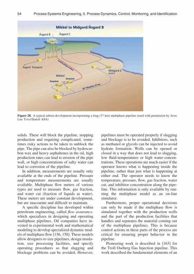
6.5. Management of Multiphase and SubseaOil Production . . . . . . . . . . . . . . . . . 53
6.6. The On-Line Facility Simulator. . . . 556.7. Conclusion and Future Directions . . 56
1. Introduction
The focus of this keyword is on the exciting fieldof process dynamics, process control, processmonitoring and process identification. This is avery broad field which is applied all across theprocess systems engineering (PSE) community.This keyword is structured such that it has focuson a number of key areas within this field.
InChapter2specialattentionispaidtoprocessmonitoring applications and development inpharmaceutical production and food production.There have beenmajor changes in those applica-tion areas, where the introduction of on-linemeasurement systems has received quite someattention in recentyears. Process instrumentationisbrieflycoveredingeneral terms, followedbyanoverview of some of the most frequently usedmonitoring tools. Short case studies illustrate theapplication of those tools.
Chapter 3 is introduced bymeans of standarddefinitions and terms. Key publications onplant-wide control are briefly summarized, fol-lowed by a comparison and critical discussion oftwo systematic procedures for design of plant-wide control systems. Most of the plant-widecontrol ideas can be transferred to batchproduction systems.
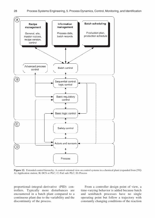
Chapter 4 focuses on batch production sys-tems, for example, in the pharmaceutical and thepolymer production industry. Following a basicdefinition of a batch production system, com-monmethods for batch productionmanagementare introduced. Quality control of batch produc-tion systems is crucial in order to obtain anefficient production system, and thereforemeth-ods and tools for inferring information aboutbatch production processes are briefly describedas well. Finally, optimal operation of singlebatch processes and batch to batch control areintroduced.
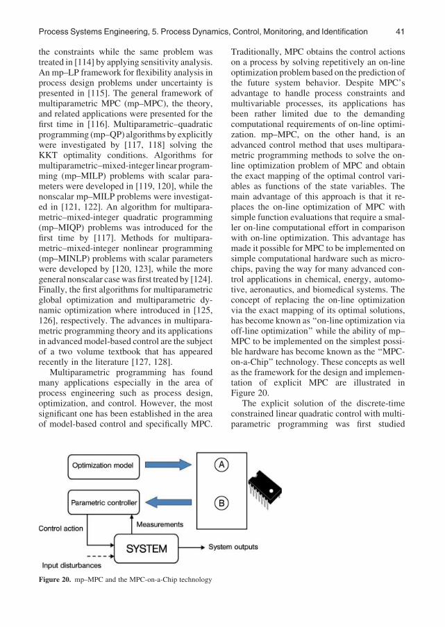
Chapter 5, on multiparametric programmingand its application within model predictive con-trol (MPC), starts with providing an overview ofthe most important developments in this area.The theory behind multiparametric program-ming is introduced, and its importance for thepractical application of MPC and ‘‘MPC on achip’’ technology is highlighted through a fewillustrative examples. This section ends with ashort discussion of future developments in thearea.
The Chapter 6 focuses on on-line applica-tion, since dynamic simulators are increasinglyused within the operation of chemical and pe-troleum production processes, to name a few
2 Process Systems Engineering, 5. Process Dynamics, Control, Monitoring, and Identification
examples. Starting from the 1980s, the contri-bution provides a brief historical perspective ofdynamic process modeling, followed by thedescription of the main software requirementsfor a typical architecture that allows on-linesimulation. Technical and organizational chal-lenges in using on-line simulation are highlight-ed, and applications of the technology aredescribed.
2. Process Monitoring
2.1. Introduction
Monitoring process performance is a criticalrequirement in any manufacturing process asproducing quality products within specificationreproducibly is a prerequisite of an economi-cally viable process. Without effective moni-toring and control strategy, as key requisite, acapable manufacturing process, could not besuccessful. Monitoring is essential for variousaspects of the control strategy–the quality of rawmaterials is usually tested on intake, processequipment often has to be rigorously qualified(e.g., in the highly regulated pharmaceutical orfood industries), environment is controlled byimplementing manufacturing-area classifica-tion where relevant, waste is treated prior torelease and the quality of the final product istested before release. Initiatives, such as qualityby design (QbD) and a supporting enablingtechnology of process analytical technology(PAT) championed by the US Food and DrugAdministration (FDA) in the pharmaceuticalindustry, aim to shift the focus for manufactur-ing from end-product quality testing to buildingthe quality in the process. Such a shift in em-phasis would not be possible without reliableand effective monitoring. Indeed PAT has beendefined as ‘‘a system for designing, analyzing,and controlling manufacturing through timelymeasurements (that is, during processing) ofcritical quality and performance attributes ofraw and in-process materials and processes,with the goal of ensuring final product quali-ty’’ [1]. Traditional process control strategiesbased upon information from laboratory assaysand supervisory computer systems (SCADA)are routinely used to regulate process operationand correct for disturbances resulting from raw
material variations through to production plantvariations. If PAT can provide additional infor-mation on disturbances and deviations, givinggreater plant insight, then the effects of distur-bances can be reduced and quality control tight-ened. However, greater benefits are to be gainedby the systematic use of PAT tools in processdevelopment to increase fundamental under-standing and more robust definition of the de-sign and control space of the process operation.
An analogy in the food industry in terms ofthe importance of effective monitoring proce-dures can be seen in the hazard analysis criticalcontrol point (HACCP) food safety standard,which is now widely incorporated into nationalfood safety legislation of many countries. Theseven basic principles of HACCP implementa-tion consist of [2]:
1. Conduct hazard analysis, considering all in-gredients, processing steps, handling proce-dures, and other activities involved in afoodstuff’s production
2. Identify critical control points (CCPs)3. Define critical limits for ensuring the control
of each CCP4. Establishmonitoringprocedures todetermine
if critical limits have been exceeded anddefine procedure(s) for maintaining control
5. Define corrective actions to be taken if con-trol is lost (i.e., monitoring indicates thatcritical limits have been exceeded)
6. Establish effective documentation andrecord-keeping procedures for developedHACCP procedure
7. Establish verification procedures for routine-ly assessing the effectiveness of the HACCPprocedure, once implemented
Clearly effective monitoring is critical toensuring product quality regardless of the typeof manufacturing industry. Essential compo-nents of effective monitoring include represen-tative measurement and a robust representationof the obtained information, allowing appropri-ate action to be taken.
2.2. Critical Process ParameterMeasurement
A complete review of specific process instru-mentation for critical parametermeasurement is
Process Systems Engineering, 5. Process Dynamics, Control, Monitoring, and Identification 3
beyond the scope of this section and the empha-sis will be placed on the characteristics ofmeasurements to be used in a critical parametercontrol scheme. These characteristics raiseimportant questions that must be answered priorto sensor specification and they lead to theestablishment of specific protocols that need tobe followed during sensor use. Such character-istics would be equally applicable to establishedas well as emerging PAT measurementmethodologies. The key considerations for asensor are:
Accuracy and Resolution. A useful sensorprovides measurement at an appropriate accu-racy for the control task. If, for example, atemperature is to be controlled in the range of�0.1 �C then the measurement must be signifi-cantly more accurate than that. If that was notthe case, the actual process may be subject tolarger deviations, although it may appear thatthe process is controlled within this range.
Precision is the probability of obtaining thesame value with repeated measurements on thesame system and it is particularly important inthe longer term operations. For instance, sensordrift from calibration can cause deterioration insystem performance because the desired valuesare not achieved. Drift is often inevitable, so itis important to know the rates of likely drift sothat recalibration can be performed asnecessary.
Sensitivity is defined as the ratio betweenthe sensor output change DS and the givenchange in the measured variable Dm (sensitivityS ¼ DS/Dm). If the critical control parametervalue changes, it is important that the sensorresponds to such a change.
Reliability. Sensors provide informationwhich is acted upon either by process operatorsin a ‘‘human in the loop’’ control scheme ordirectly by closed-loop control schemes. Whenoperators use the information, there is someopportunity for human interpretation of theresults. Failed sensors are more difficult todetect in a hardware-based closed-loop scheme.If the information is essential and a sensor fails,then implications on operation can be severe.Reliability is a function of the failure rate, of the
failure type, ease ofmaintenance and repair, andphysical robustness. Redundancy and plannedmaintenance programs to maintain the sensorsare required to maintain reliability.
Response time is defined as the time re-quired for a sensor output to change from itsprevious state to a final settled value within atolerance band of the correct new value. Thedynamic sensor characteristics are important asthe sensor must respond significantly faster thanthe process. If a sensor has a long response timeit may indicate an ‘‘average’’ value rather thanthe actual process value.
Practicality. The environment within a pro-cess may be particularly demanding—forinstance, the sensors may be exposed to hightemperatures or pressures. Whilst a sensor mayin theory measure the variable of interest inideal conditions, the range of the operationalenvironment could render it incapable of func-tioning or may influence reliability.
Cost. Sophisticated instrumentation is nowavailable for process monitoring with PAT, butthe price can be high. However, the benefitsgained can be significant if sensor informationleads to raw material/resource savings or in-creases productivity. A cost benefit analysisshould be performed to assess whether theinstrumentation is appropriate.
A significant issue to be addressed in effec-tive monitoring is the placement of a sensor(Fig. 1) as it influences the frequency of avail-able measurements. Theory dictates that for a
Figure 1. Sensor classification based on placement andspeed of response
4 Process Systems Engineering, 5. Process Dynamics, Control, Monitoring, and Identification
measurement to be of value it must be sampledabove a certain minimum frequency. Often in-struments are used on-line (say temperature orpH) or they can be multiplexed to save cost, butthe frequency of information supply is limitedbecause the instruments must serve severalvessels (e.g., mass spectrometer measure-ments). However, it is off-line sample analysiswhere problems with low frequency measure-ment are most likely to arise.
Initiatives such as PAT lead to increased useof sophisticated sensor technology, such as nearinfrared spectroscopy (NIR), which requiresmore powerful data interpretation and monitor-ing tools.
2.3. Monitoring Tools
During the 1920s, the control charting method-ology as the fundamental tool to understand andaddress variability, the foundation of so-calledstatistical process control, was developed [3].Visualizing the variability is central to its re-duction and statistical tools, such as cause andeffect diagram, flow chart, Pareto chart, histo-gram, run chart, scatter diagram, and controlcharts, are often used. Histograms, flow charts,run charts, and scatter diagram compile the datato show the overall picture while Pareto dia-grams are used to show problem areas. Howev-er, these methods do not indicate limits withinwhich the process is to operate. The univariateSPC methodology uses charts with upper con-trol limits known as ‘‘UCL’’, lower controllimits known as ‘‘LCL’’ and means denoted as�X or �R for individual process variables. Thebasic principles of control charts, control limitsettings, moving average charts, exponentiallyweighted moving average (EWMA) and cumu-lative sum (or CUSUM) control charts are de-scribed in [4] and illustrated by means of a casestudy of a mean particle size monitoring in acrystallization unit operation in the pharmaceu-tical industry [4].
Whilst univariate SPC can be very effectiveand has been used widely, it fails to account forthe interactions between process variables andthus to recognize off-specification behavior.Also, univariate charts may indicate off-specification behavior in terms of one processvariable, but to identify the cause of the fault
conditions the interpretation of multiple chartsis required. Finally, nonsteady-state behavior,process dynamics, time delays, etc. cause uni-variate charts to be inappropriate. Since mostindustries collect large amounts of data, multi-variate statistical process control procedures arenow considered to be an appealing approach toprocess monitoring and variability reduction.
2.3.1. Data Compression Methods forMultivariate Statistical Process Control(MSPC)
Multivariate SPC methods [5, 6] are based onfundamental concepts of principal componentanalysis (PCA) and partial least squares (PLS),also known as projection to latent structures.PCA [7] generates a new group of uncorrelatedvariables (principal components, PCs). The ap-proach transforms matrix containing measure-ments from n process variables, [X], into amatrix of mutually uncorrelated PCs, tk (wherek ¼ 1 to n) which are transforms of the originaldata into a new basis defined by a set of orthog-onal loading vectors, pk. The individual valuesof the principal components are called scores.The transformation is defined by Equation (1):
½X� ¼Xnp< n
k¼1
tkpTkþE ð1Þ
The loadings are the eigenvectors of the datacovariance matrix, XTX. The tk and pk pairs areordered so that the first pair captures the largestamount of variation in the data and the last paircaptures the least. This means that fewer PCsare required to describe the relationship thanoriginal process variables. The compression ofdata allows a visualization of the compresseddata for the purpose of feature extraction andthus enables the analysis of interacting processvariables that are the cause of processdeviations.
PLS [8] is a tool suitable whenever plantvariables can be partitioned into cause (X) andeffect (Y) values. The algorithm operates byprojecting the cause and effect data onto anumber of latent variables and then modellingthe relationships between these new variables(the so-called inner models) by single-input–single-output linear regression as described by
Process Systems Engineering, 5. Process Dynamics, Control, Monitoring, and Identification 5
Equations (2) and (3):
X ¼Xnp< nx
k¼1
tkpTkþE and Y ¼
Xnp< nx
k¼1
ukqTkþF� ð2Þ
where E and F* are residual matrices, np is thenumber of inner components that are used in themodel and nx is the number of causal variables.
uk ¼ bktkþek ð3Þ
where bk is a regression coefficient, and ek refersto the prediction error.
2.3.2. Multiway MSPC
Batch processes typically exhibit nonlinearcharacteristics that may limit the effectivenessof conventional linear PCA and PLS
procedures. Whilst nonlinear MSPC techniqueshave been developed and applied successful-ly [9], the transformation of batch data hasproved to be a more effective option. The mostcommon form of data transformation, termedmultiway PCA and PLS, was initially proposedby [5]. Since then, for example, the techniquewas applied by [10] to monitor faults in auto-motive engine performance. The detection offaults by measuring particular chemicals frommixtures using electronic nose based on gaschromatography-mass spectrometry (GC-MS)was investigated by [11].
The concept of multiway PCA and PLS is arelatively straightforward extension where de-viations frommean trajectories rather than stea-dy-state are considered [5]. Figures 2 and 3illustrate the principle for a typical set of
Figure 2. Typical data structure in a batch manufacturing processa) Raw materials; b) Online data; c) Quality data; d) DSP data
Figure 3. One possible multiway decomposition of on-line dataBatch 1: time ¼ 1. . .n1; Batch 2: time ¼ 1. . .n2; Batch 3: time ¼ 1. . .n3n1<n3<n2
6 Process Systems Engineering, 5. Process Dynamics, Control, Monitoring, and Identification
operational process data where data of varioussize and frequency may be collected at variousstages of processing.
Quality data on raw materials used in severalbatches, fromwhich data ismonitored over timefrom several sensors will need to be linked withquality data monitored during the batch at vari-ous frequencies for various quality attributesand merged with on-line data available fromdownstream processing unit operations.
Given that the duration of each batch is likelyto differ, as indicated in Figure 3, the data fromeach batch is often considered only until theshortest run length. For each variable the meantrajectory over all the batches used in modelbuilding is calculated and removed from eachprocess measurement. This effectively removesthe major nonlinearity from the data and leavesa zero mean trajectory for each variable. Theindividual data matrices from each batch areunfolded into a single unfolded data matrix asdepicted in Figure 3 and PCA can be applied tothis unfolded data matrix.
2.4. Seed Quality Monitoring CaseStudy
A typical example of the data structure depictedin Figure 2 is taken from the bioprocessingindustry. In order to monitor the quality of seedcultivations used for starting the manufacturingprocess in a range of valuable biological pro-ducts, such as antibiotics, a number of processvariables are measured. These include respira-tory data, as well as information about theoperating conditions, such as agitation, pH,temperature, etc. In this case study, 20 lots ofdata from the seed stage of pilot-scale antibioticcultivations were available and only the airflowand respiratory data were used in analyses asother variables were tightly controlled. The datamatrix forMPCA analysis was then constructedas indicated in Figure 3. Figure 4 depicts the plotof the resulting PC1 against PC2 and illustratesthe degree of separation within this cluster. InFigure 4 (o) represent batches that ultimatelyresulted in low final stage productivity while(þ) represent the high productivity batches.Tentative clusters of high- and low-productivitybatches can be seen even at cursory inspection,for example, along the vertical line representing
the PC2 axis. Although, based on such a simpleseparation, three of the low final-productivityseed batches would cluster within the ‘‘high’’cluster, this may be an entirely plausible sce-nario. The seed could have had the same char-acteristics as those seeds ultimately resulting inhigh productivity, i.e., a ‘‘good’’ seed, but pro-blems could have arisen during the final fer-mentations, which potentially could have led toreduced productivity.
These results demonstrate that it is possibleto extract features from seed data that relate tothe final productivity and thus to indicate thequality of a particular seed before inoculatingthe production vessel at the pilot plant scale.
2.5. Alternative Methods
Unfolding the data and reducing the length ofeach batch to that of the shortest one maysignificantly reduce the monitoring effective-ness of MPCA and a number of alternativemethods have been developed over the yearsto address this issue. For example, see [12] foran application to on-line steady-state identifica-tion in polymer injection molding start-up pro-cess. There are also a number of alternativemethods of data interpretation, such as parallelfactor analysis (PARAFAC). The performanceof several algorithms for fitting the PARAFACmodel was compared by [13]. These includealternating least squares (ALS), direct trilinear
Figure 4. Plot of PC1 vs PC2 of a MPCA model for seedquality monitoringa) High productivity; b) Low productivity98% variance captured 5PCs
Process Systems Engineering, 5. Process Dynamics, Control, Monitoring, and Identification 7
A further category of methods include non-linear data representation techniques rangingfrom the nonlinear forms of the multivariatedata analysis methods above to the variousforms of artificial neural networks (ANN) thathave been proven effective in monitoring avariety of processes ranging from fermenta-tions [14], object tracking [15], wastewatertreatment [16] to monitoring the thermal per-formance of heat exchangers [17].
One particular type of ANN, referred to asradial basis function (RBF) network, has beenproven to provide an efficient monitoring tool.RBF neural networks consist of three layers ofnodes interconnected in a feed-forward manner,as shown in Figure 5 for two outputs and alimited interconnection illustrated to retain areasonable level of picture clarity.
The first layer distributes the input data intothe hidden layer of the network. The hiddennodes perform a nonlinear transformation of theinput data [18]. Usually, the Gaussian functionis used, as described by the Equation (4):
ah ¼ exp�kx�chk2
b2h
" #ð4Þ
where ah is the activation of the hth processingunit in the hidden layer in response to the
input vector ‘x ¼ fx1; . . . ; xng’; ch and bh rep-resent the position of the center and the clusterwidths in the input space of the unit h,respectively.
The hidden layer outputs are weighted andsummed in the output nodes. The response of thejth output node, yj, is given by Equation (5).
yj ¼XHþ1
h¼1
Wj;hahþu ð5Þ
where Wj;h is the weight between the hiddennode h and the output node j. The bias node isrepresented by u and has the value of 1 [19].
The major advantage of neural networks isthat they are able to ‘‘learn’’ from the informa-tion that is presented. This means, however, thata suitable training data set is crucial for a goodperformance. The importance of the size andquality of the training data set in ANNmodelinghas been reported extensively in literature [20].Other important issues in the development ofRBF models are the selection of the networkinputs and the most suitable architecture, i.e.,the number of RBF units and the number ofnearest neighbors to be used. Whilst the selec-tion of inputs is usually accomplished by usingprocess knowledge [21], prediction errors andcross validation are most frequently used toselect the network topology [19].
Once the topology is defined, the networkcan be trained, i.e., the unit centers, unit widths,and weights are calculated, for example, byusing MOODY and DARKEN’s three stepapproach [22]:
1. The unit centers, c, are determined by the k-means clustering algorithm, which dividesthe training data into subsets. Each subset isrelated to a cluster center, according to thesimilarities of the data. These similarities aredetermined by the distance between two datapoints. The algorithm minimizes an objec-tive function E, which is usually the totalsquared Euclidean distance between the Ktraining points in each cluster and the Hcluster centers, according to Equation (6):
E ¼XHh¼1
XKk¼1
Mhkkch�xkk2 ð6Þ
In Equation (6), Mhk is a H � K matrixcalled the membership function or cluster
Figure 5. Radial basis function (RBF) neural networkarchitecturea) Input layer; b) Hidden layer; c) Output layer
8 Process Systems Engineering, 5. Process Dynamics, Control, Monitoring, and Identification
partition. Each column contains a single 1that identifies the processing unit to which agiven training point belongs, and zeros areassigned elsewhere [21].
Once this is achieved, each cluster isassociated with one RBF unit and the clustercenters become the unit centers c. Eachcenter is then comparedwith the input vectorand the corresponding unit is activated ac-cording to the distance between the networkinput vector and the center.
2. After determining the unit centers, a P-near-est neighbors heuristic (Eq. 7) can be used tofind the unit widthssh. The unit width shouldbe determined so that it is greater than thedistance to the nearest unit center. Thisallows the hidden unit to activate at leastanother hidden unit. Consequently, any pointwithin the bounds of that unit will be able tosignificantly activate more than one unit,improving the fit of the desired outputs.
sh ¼ 1
p
Xpm¼1
kc�zmk2 !1/2
ð7Þ
where ‘zm’ represents the P-nearest neigh-bors of c.
3. The weights of the output layer are thencalculated using a least squares-based meth-od. The objective is to find the weights thatminimize the squared norm of the residuals.The output layer nodes simply sum the out-puts from the hidden layer.
After determining the parameters of the net-work, the local reliability can be measured bycalculating the confidence limits for the modelestimation at a given test point. This is the resultof the weighted average of the local confidenceintervals calculated for each RBF unit [18, 19].
2.6. RBF-Based Monitoring CaseStudy
RBF neural network modeling has been used tomonitor a range of different processes. In thisexample, it is used to detect deviations in large-scale production of penicillin. A number offactors influence the behavior of a large-scalefermentation and a dynamic and nonlinearcharacter of the bioprocess mean that simple
monitoring of individual process variables doesnot allow the detection of a developing processdeviation, unless there is a severe, obvious fault.However, detecting deviations early in the pro-cess is essential in order to ensure that theprocess is returned to normal behavior and toprevent economic consequences due to lowerproductivity or even a complete loss of thewhole batch.
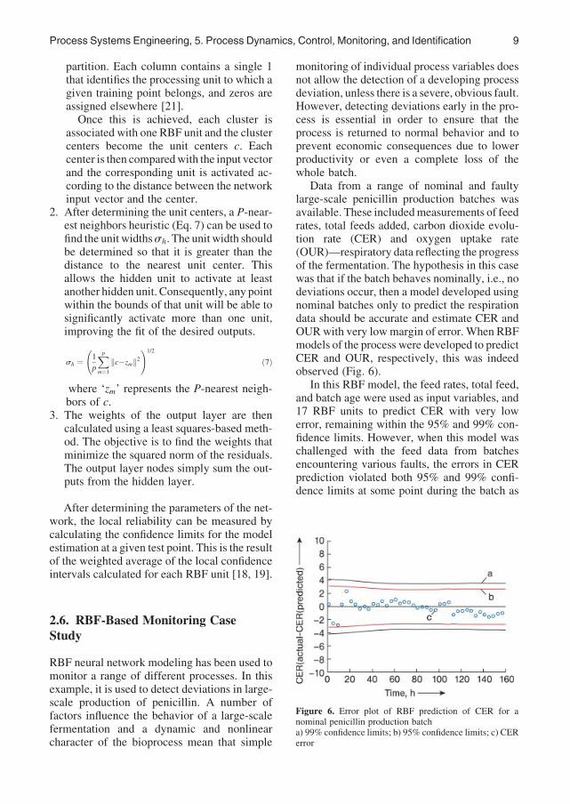
Data from a range of nominal and faultylarge-scale penicillin production batches wasavailable. These includedmeasurements of feedrates, total feeds added, carbon dioxide evolu-tion rate (CER) and oxygen uptake rate(OUR)—respiratory data reflecting the progressof the fermentation. The hypothesis in this casewas that if the batch behaves nominally, i.e., nodeviations occur, then a model developed usingnominal batches only to predict the respirationdata should be accurate and estimate CER andOURwith very lowmargin of error. When RBFmodels of the process were developed to predictCER and OUR, respectively, this was indeedobserved (Fig. 6).
In this RBF model, the feed rates, total feed,and batch age were used as input variables, and17 RBF units to predict CER with very lowerror, remaining within the 95% and 99% con-fidence limits. However, when this model waschallenged with the feed data from batchesencountering various faults, the errors in CERprediction violated both 95% and 99% confi-dence limits at some point during the batch as
Figure 6. Error plot of RBF prediction of CER for anominal penicillin production batcha) 99% confidence limits; b) 95% confidence limits; c) CERerror
Process Systems Engineering, 5. Process Dynamics, Control, Monitoring, and Identification 9
shown in Figure 7 for five faulty batches sepa-rated by vertical lines.
The violations of the confidence limits couldtheoretically be caused by the RBF model ex-trapolating outside the range of the input dataused for training (a frequent shortfall of ANNmethodology) or by a biological variabilitycausing real deviations of the process from thenominal behavior. The benefit of using RBFmodels is that check on maximum activity andprobability density [19] provides a measure ofextrapolation. In this case it clearly confirmedthat the reason for the violation of the confi-dence limits is biological process variability.
However, establishing the reason for suchdeviations is not a straightforward matter. Oneof the limitations of ANN methodology is thefact that the interpretation of causal relation-ships is more difficult than with some of themore established linear methods, such as PCAand PLS. In some areas of bioprocessing, e.g.,the manufacture of biologics for human con-sumption, the simple indication of process de-viation, regardless of the underlying reason, isall that is required, as the strict regulatoryrequirements mean that the batch will have tobe terminated and cannot be remedied. In suchcircumstances in particular the ANN-basedmonitoring can prove very effective.
There are a large number of other types ofANNmodels developed specifically for estima-tion of process variables or fault detection andclustering/classification. The various forms of
neural networks used in diverse applicationspreclude detailed description of this methodol-ogy here, but extensive literature is availableboth on the principles and their variousapplications.
3. Plantwide Control
3.1. Introduction
A chemical plant may have thousands of mea-surements and control loops. By the term plant-wide control it is not meant the tuning andbehavior of each of these loops, but rather thecontrol philosophy of the overall plant withemphasis on the structural decisions:
. Selection of controlled variables (CVs,‘‘outputs’’)
. Selection of manipulated variables (MVs,‘‘inputs’’)
. Selection of (extra) measurements
. Selection of control configuration (structureof overall controller that interconnects thecontrolled, manipulated, and measuredvariables)
. Selection of controller type (proportional–integral–derivative (PID), decoupler, modelpredictive control (MPC), linear–quadratic–Gaussian (LQG), ratio, etc.)
In practice, the control system is usuallydivided into several layers, separated by timescale (see Fig. 8).
Plantwide control thus involves all the deci-sions necessary to make a block diagram (usedby control engineers) or a process and instru-mentation diagram (used by process engineers)for the entire plant, but it does not involve theactual design of each controller.
In any mathematical sense, the plantwidecontrol problem is a formidable and almosthopeless combinatorial problem involving alarge number of discrete decision variables, andthis is probably why the progress in the area hasbeen relatively slow. In addition, the problemhas been poorly defined in terms of its objective.Usually, in control, the objective is that thecontrolled variables (CVs, outputs) should re-main close to their setpoints. However, whatshould be controlled? Which CVs? The answer
Figure 7. Error plot of RBF prediction of CER for fivefaulty penicillin production batches separated by verticallinesa) 99% confidence limits; b) 95% confidence limits; c) CERerror
10 Process Systems Engineering, 5. Process Dynamics, Control, Monitoring, and Identification
lies in considering the overall plant objective,which normally is to minimize the economiccost (¼ maximize profit) while satisfying oper-ational constraints imposed by the equipment,market demands, product quality, safety, envi-ronment, and so on. The truly optimal ‘‘plant-wide controller’’ would be a single centralizedcontrollerwhich at each time step collects all theinformation and computes the optimal changesin the manipulated variables (MVs). Althoughsuch a single centralized solution is foreseeableon some simple processes, it seems to be safe toassume that it will never be applied to anynormal-sized chemical plant. There are manyreasons for this, but one important is that inmostcases one can obtain acceptable control perfor-mance with simple structures where each con-troller block only involves a few variables, andsuch control systems can be designed and tunedwith much less effort, especially when it comesto themodeling and tuning effort. After all, mostreal plants operate well with simple control
structures. So how are systems controlled inpractice? The main simplification is to decom-pose the overall control problem into manysimpler control problems. This decompositioninvolves two main principles:
1. Decentralized (local) control. This ‘‘hori-zontal decomposition’’ of the control layeris mainly based on separation in space, forexample, by using local control of individualprocess units
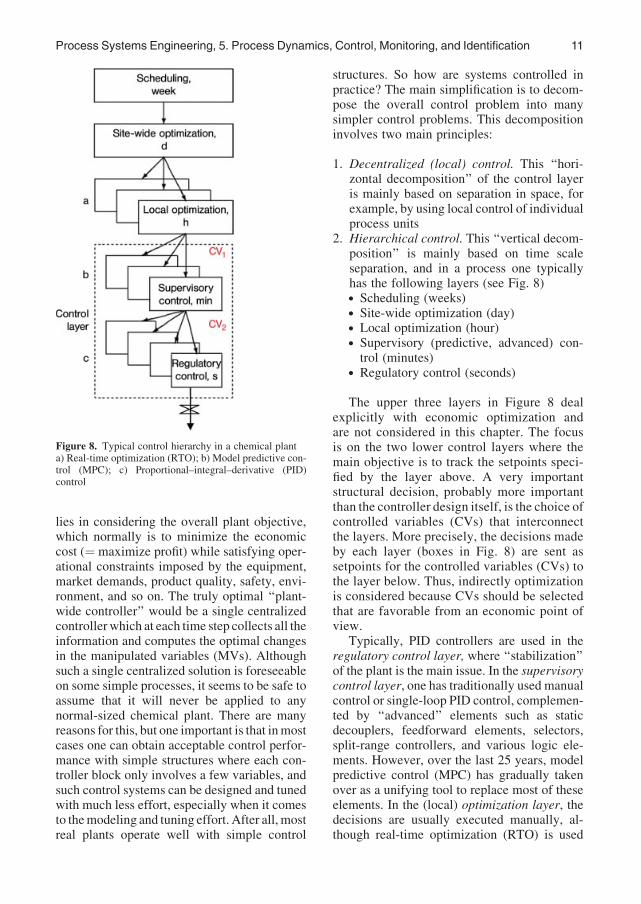
2. Hierarchical control. This ‘‘vertical decom-position’’ is mainly based on time scaleseparation, and in a process one typicallyhas the following layers (see Fig. 8). Scheduling (weeks). Site-wide optimization (day). Local optimization (hour). Supervisory (predictive, advanced) con-trol (minutes)
. Regulatory control (seconds)
The upper three layers in Figure 8 dealexplicitly with economic optimization andare not considered in this chapter. The focusis on the two lower control layers where themain objective is to track the setpoints speci-fied by the layer above. A very importantstructural decision, probably more importantthan the controller design itself, is the choice ofcontrolled variables (CVs) that interconnectthe layers. More precisely, the decisions madeby each layer (boxes in Fig. 8) are sent assetpoints for the controlled variables (CVs) tothe layer below. Thus, indirectly optimizationis considered because CVs should be selectedthat are favorable from an economic point ofview.
Typically, PID controllers are used in theregulatory control layer, where ‘‘stabilization’’of the plant is the main issue. In the supervisorycontrol layer, one has traditionally used manualcontrol or single-loop PID control, complemen-ted by ‘‘advanced’’ elements such as staticdecouplers, feedforward elements, selectors,split-range controllers, and various logic ele-ments. However, over the last 25 years, modelpredictive control (MPC) has gradually takenover as a unifying tool to replace most of theseelements. In the (local) optimization layer, thedecisions are usually executed manually, al-though real-time optimization (RTO) is used
Figure 8. Typical control hierarchy in a chemical planta) Real-time optimization (RTO); b) Model predictive con-trol (MPC); c) Proportional–integral–derivative (PID)control
Process Systems Engineering, 5. Process Dynamics, Control, Monitoring, and Identification 11
for a few applications, especially in the refiningindustry.
The following decisions must be made whendesigning a plantwide control strategy:
1. Decision 1: Select ‘‘economic’’ (primary)controlled variables (CV1) for the supervi-sory control layer
2. Decision 2: Select ‘‘stabilizing’’ (secondary)controlled variables (CV2) for the regulatorycontrol layer
3. Decision 3: Locate the throughput manipu-lator (TPM), that is, where to set the produc-tion rate
4. Decision 4: Select pairings for the stabilizinglayer, that is, pair inputs (valves) and con-trolled variables (CV2).
Decisions 1 and 2 are illustrated in Figure 9,where the matrices H and H2 represent aselection, or in some cases a combination, ofthe available measurements y.
This chapter deals with continuous operationof chemical processes, although many of thearguments hold also for batch processes.
3.2. Previous Work
Over the years, going back to the early work ofBUCKLEY [23] from DuPont, several approaches
have been proposed for dealing with plantwidecontrol issues. Nevertheless, taking into accountthe practical importance of the problem, theliterature is relatively scarce. LARSSON andSKOGESTAD [24] provide a good review anddivide into two main approaches. First, thereare the process-oriented (engineering or simu-lation-based) approaches of [25–30]. One prob-lem here is the lack of a really systematicprocedure and that there is little considerationof economics. Second, there is the optimizationor mathematically oriented (academic) ap-proaches of [31–35]. The problem here is thatthe resulting optimization problems are intrac-table for a plantwide application. Therefore, ahybrid between the two approaches is morepromising [24, 36–40].
The first really systematic plantwide controlprocedure was that of LUYBEN et al. [28, 29]which has been applied in a number of simula-tion studies. LUYBEN’s procedure consists of thefollowing nine steps
. L1: Establish control objectives
. L2: Determine control degrees of freedom
. L3: Establish energy management system
. L4: Set the production rate (decision 3)
. L5:Control product quality and handle safety,environmental, and operational constraints
. L6: Fix a flow in every recycle loop andcontrol inventories
. L7: Check component balances
. L8: Control individual unit operations
. L9:Optimize economics and improve dynam-ic controllability
‘‘Establish control objectives’’ in step L1does not lead directly to the choice of controlledvariables (decisions 1 and 2). Thus, in LUYBEN’sprocedure, decisions 1, 2, and 4 are not explicit,but are included implicitly in most of the steps.Even though the procedure is systematic, it isstill heuristic and ad hoc in the sense that it is notclear how the authors arrived at the steps or theirorder. A major weakness is that the proceduredoes not include economics, except as an after-thought in step L9.
In this chapter, the seven-step plantwidecontrol procedure of SKOGESTAD [24, 39] isdiscussed. It was inspired by the LUYBEN proce-dure, but it is clearly divided into a top-downpart, mainly concerned with steady-state
Figure 9. Block diagram of control hierarchy illustratingthe selection of controlled variables (H andH2) for optimaloperation (CV1) and stabilization (CV2)
12 Process Systems Engineering, 5. Process Dynamics, Control, Monitoring, and Identification
economics, and a bottom-up part, mainly con-cerned with stabilization and pairing of loops.SKOGESTAD’s procedure consists of the followingsteps:
1. Top-down part (focus on steady-state opti-mal operation). S1: Define operational objectives (eco-nomic cost function J and constraints)
. S2: Determine the optimal steady-stateoperation conditions
. S4: Select the location of the throughputmanipulator (TPM) (decision 3)
2. Bottom-up part (focus on the control layerstructure). S5: Select the structure of the regulatory(stabilizing) control layer (decisions 2and 4)
. S6: Select the structure of the supervisorycontrol layer
. S7: Select structure of (or need for) theoptimization layer (RTO)
The top-down part (steps 1–4) is mainlyconcerned with economics, and steady-stateconsiderations are often sufficient. Dynamicconsiderations are more important for steps4–6, although steady-state considerations areimportant also here. This means that it is impor-tant in plantwide control to involve engineerswith a good steady-state understanding of theplant. A detailed analysis in step S2 and step S3requires that one has a steady-state model avail-able and that one performs optimizations for thegiven plant design (‘‘rating mode’’) for variousdisturbances.
3.3. Degrees of Freedom forOperation
The issue of degrees of freedom for operation,or control degrees of freedom, is often confus-ing and not as simple as one would expect.One issue is that the degrees of freedomchange depending on where one is in the con-trol hierarchy. This is illustrated in Figures 8and 9, where the degrees of freedom inthe optimization and supervisory control
layers are not the physical degrees of freedom(valves), but rather the setpoints for thecontrolled variables in the layer below. Thecontrol degrees of freedom are often referredto as manipulated variables (MVs) or inputs.The physical degrees of freedom (dynamicprocess inputs) are called ‘‘valves’’, becausethis is usually what they are in processcontrol.
Steady-State DOFs (u). A simple approachis to first identify all the physical (dynamic)degrees of freedom (valves). However, becausethe economics usually depend mainly on thesteady-state, variables that have no or negligibleeffect on the economics (steady-state) should besubtracted, such as inputs with only a dynamiceffect or controlled variables (e.g., liquid levels)with no steady-state effect.
#steady-state degrees of freedom ðuÞ¼ #valves�#variables with no steady-state effect
For example, even though a heat exchangermay have a valve on the cooling water and inaddition have bypass valves on both the hot andcold side, it usually has only one degree offreedom at steady-state, namely the amount ofheat transferred, so two of these three valvesonly have a dynamic effect from a control pointof view.
In addition, we need to exclude valves thatare used to control variableswith no steady-stateeffect (usually, liquid levels). This is illustratedin the following example.
Example: DOFs for Distillation: A simpledistillation column has six dynamic degrees offreedom (valves): feed F, bottom product B,distillate product D, cooling, reflux L, and heatinput. However, two degrees of freedom (e.g., Band D) must be used to control the condenserand reboiler levels (MB andMD) which have nosteady-state effect. This leaves four degrees offreedom at steady-state. For the common casewith a given feed flow and a given columnpressure, only two steady-state degrees of free-dom remain. Thus, for the economic analysis instep S3, 2 controlled variables (CV1) need to beselected associated with these. Typically, thesewill be the top and bottom composition, but notalways.
Process Systems Engineering, 5. Process Dynamics, Control, Monitoring, and Identification 13
3.4. SKOGESTAD’s Plantwide ControlProcedure
Going through the SKOGESTAD procedure inmore detail, an existing plant is considered andit is assumed that a steady-state model of theprocess is available.
The top-down part is mainly concerned withthe plant economics, which are usually deter-mined primarily by the steady-state behavior.Therefore, although one is concerned aboutcontrol, steady-state models are usually suffi-cient for the top-down part.
Step S1: Define Operational Objectives(Cost J and Constraints). A systematic
approach to plantwide control requires that firstthe operational objectives are quantified interms of a scalar cost function J [$/s] that shouldbe minimized (or equivalently, a scalar profitfunction, P ¼ �J, that should be maximized).This is usually not very difficult, and typically itis:
Fixed costs and capital costs are not included,because they are not affected by plant operationon the time scale considered (ca. 1 h). The goalof operation (and of control) is to minimize thecost J, subject to satisfying the operationalconstraints (g � 0), including safety and envi-ronmental constraints. Typical operational con-straints are minimum and maximum values onflows, pressures, temperatures, and composi-tions. For example, all flows, pressures, andcompositions must be nonnegative.
Step S2: Determine the Steady-State Opti-mal Operation. Before the control system
is designing the optimal way of operating theprocess should be considered. For example, avalve (e.g., a bypass) should always be closed.This valve should then not be used for (stabiliz-ing) control unless one is willing to accept theloss implied by ‘‘backing off’’ from the optimaloperating conditions.
To determine the steady-state optimal oper-ation, a steady-state model should be obtained.Then the degrees of freedom and expecteddisturbances need to be identified, and optimi-zations for the expected disturbances should beperformed:
1. Identify steady-state degrees of freedom (u):To optimize the process, the steady-statedegrees of freedom (u) have to be identifiedas has already been discussed. Actually, it isthe number of u’s which is important, be-cause it does not really matter which vari-ables are included in u, as long as they makeup an independent set
2. Identify important disturbances (d) and theirexpected range: Next, the expected range ofdisturbances (d) for the expected future op-eration have to be identified. The most im-portant disturbances are usually related to thefeed rate (throughput) and feed composition,and in other external variables such as tem-perature and pressure of the surroundings.Furthermore, changes in specifications andconstraints (such as purity specifications orcapacity constraints) and changes in para-meters (such as equilibrium constants,rate constants and efficiencies) should beincluded as disturbances. Finally, the ex-pected changes in prices of products, feeds,and energy need to be included as‘‘disturbances’’.
3. Optimize the operation for the expecteddisturbances: Here, the disturbances (d) arespecified and the degrees of freedom(uopt(d)) are varied in order to minimize thecost (J), while satisfying the constraints. Themain objective is to find the constraintsregions (sets of active constraints) and theoptimal nominal setpoints in each region.
Mathematically, the steady-state optimiza-tion problem can be formulated as
minu Jðu; x; dÞsubject to:Model equations: f ðu; x; dÞ ¼ 0Operational constraints: gðu; x; dÞ � 0
Here u are the steady-state degrees of free-dom, d are the disturbances, x are the internalstates, f ¼ 0 represents the mathematical modelequations and possible equality constraints (likea given feed flow), and g � 0 represents theoperational constraints (like a maximum ornonnegative flow, or a product compositionconstraint). The process model, f ¼ 0, is oftenrepresented indirectly in terms of a commercialsoftware package (process simulator), such as
14 Process Systems Engineering, 5. Process Dynamics, Control, Monitoring, and Identification
Aspen or Hysis/Unisim. This usually results in alarge, nonlinear equation set which often haspoor numerical properties for optimization.
Together with obtaining the model, the opti-mization step S2 is often the most time consum-ing step in the entire plantwide control proce-dure. In many cases, the model may not beavailable or one does not have time to performthe optimization. In such cases a good engineercan often perform a simplified version of stepS1–S3 by using process insight to identify theexpected active constraints and possible ‘‘self-optimizing’’ controlled variables (CV1) for theremaining unconstrained degrees of freedom.
A major objective of the optimization is tofind the expected regions of active constraints.An important point is that one cannot expect tofind a single control structure that is optimalbecause the set of active constraints will changedepending on disturbances and economic con-ditions (prices). Thus, one should prepare thecontrol system for the future, by using off-lineanalysis and optimization to identify regions ofactive constraints. The optimal active con-straints will vary depending on disturbances(feed composition, outdoor temperature, prod-uct specifications) and market conditions(prices).
Generally there are two main modes of oper-ation depending on market conditions:
. Mode I: Given throughput (buyers market).This is usually the ‘‘nominal’’ mode for whichthe control system is originally set up. Usual-ly, it corresponds to a ‘‘maximize efficiency’’situation where there is some ‘‘trade-off’’between utility (energy) consumption andrecovery of valuable product, correspondingto an unconstrained optimum.
. Mode II: Maximum throughput (sellers mar-ket). When the product prices are sufficientlyhigh compared to the prices of raw materials(feeds) and utilities (energy), it is optimal toincrease the throughput as much as possible.However, as one increases the feed rate, onewill usually encounter constraints in variousunits, until eventually reaching the bottleneckwhere a further increase is infeasible.
optimal operation points found in step S2 in arobust and simple manner. To make use of allthe economic degrees of freedom (inputs u), asmany economic controlled variables (CV1) asthere are inputs (u) need to be identified. Inshort, the issue is: What should be controlled?
1. Identify candidate measurements (y) andtheir expected static measurement error (ny).In general, in the set y all inputs (valves)should be included to allow, for example, forthe possibility of keeping an input constant.
2. Select primary (economic) controlled vari-ables, CV1 ¼ Hy (decision 1), among thecandidatemeasurements (see Fig. 9), usuallyby selecting individual measurements. Oneneeds to find one CV1 for each steady-statedegree of freedom (u)
For economic optimal operation, the rules forCV1 selection are
1. Control active constraints2. For the remaining unconstrained degrees of
freedom: Control ‘‘self-optimizing’’ vari-ables with the objective of minimizing theeconomic loss with respect to disturbances
The two rules are discussed in detail below.In general, step S3 must be repeated for eachconstraint region. To reduce the need for switch-ing between regions, onemay consider using thesame CV1’s in several regions, but this is non-optimal and may even lead to infeasibility.
Control Active Constraints. In general, theobvious controlled variables to keep constantare the active constraints. The active con-straints come out of the analysis in step S2 ormay in some cases be identified based onphysical insight. The active constraints areobvious ‘‘self-optimizing’’ variables and couldbe input constraints (in the set u) or outputconstraints.
Input constraints are trivial to implement;the input is set at its optimal minimum ormaximum, so no control system is needed. Forexample, if a very old car is operated thenoptimal operation (defined as minimum drivingtime, J¼ T) may be achieved with the gas pedalat its maximum position.
For output constraints, a controller is needed,and a simple single-loop feedback controller is
Process Systems Engineering, 5. Process Dynamics, Control, Monitoring, and Identification 15
often sufficient. For example, if there exists abetter car then the maximum speed limit (say80 km/h) is likely an active constraint andshould be selected as the controlled variable(CV1). To control this, one may use a ‘‘cruisecontroller’’ (automatic control) which adjuststhe engine power to keep the car close to a givensetpoint. In this case, the speed limit is a hardconstraint and one needs to back off from thespeed limit (say to a setpoint of 75 km/h) toguarantee feasibility if there is a steady-state measurement error (ny) or a dynamic con-trol error. In general, the backoff should beminimized because any backoff results in a loss(i.e., a larger J ¼ T) which can never berecovered.
The backoff is the ‘‘safety margin’’ from theactive constraint and is defined as the differencebetween the constraint value and the chosensetpoint:
Backoff ¼ jConstraint�Setpoint j
In the car driving example: backoff¼ 5 km/h.The active constraints should be selected as
CVs because the optimum is not ‘‘flat’’ withrespect to these variables. Thus, there is often asignificant economic penalty if one ‘‘backs off’’from an active constraint, so tight control of theactive constraints is usually desired. If a con-strained optimization method is used for theoptimization, then the loss can be quantified byusing the Lagrange multiplier l associated withthe constraint:
Loss ¼ l� backoff
For input (valve) constraints, usually nobackoff is needed, unless the input for stabili-zation is used in the lower regulatory (stabiliz-ing) layer because one needs some range to useit for control. For output constraints two casesexist:
. Hard output constraints (must be satisfied atall times): Backoff¼measurement error (biasny) þ control error (dynamic)
To reduce the backoff, accurate measure-ments of the constraint outputs are necessary,and for hard output constraints one also needs
tight control with a small dynamic control error.The squeeze and shift rule for hard outputconstraints indicates: By squeezing the outputvariation, the setpoint can be shifted closer to itslimit (i.e., reduce the backoff). For soft outputconstraints, only the steady-state control errormatters, which will be zero if the controller hasintegral action.
Control ‘‘Self-optimizing’’ Variable WhichWhenHeldConstant Keeps theOperationCloseto the Optimum in spite of Disturbances. It isusually simple to identify and control the activeconstraints. Themore difficult question is:Whatshould the remaining unconstrained degrees offreedom be used for? Does it even make adifference what is controlled? The answer is‘‘yes’’!
As an example, optimal operation of a mara-thon runner is considered where the objective isto adjust the power (u) and to minimize the time(J ¼ T). This is an unconstrained problem; amarathon runner cannot simply run atmaximumspeed (u ¼ umax) as for a sprinter. A simplepolicy is constant speed (c1¼ speed), but it is notoptimal if there are disturbances (d) caused bywind or hilly terrain. A better choice is to runwith constant pulse (c2 ¼ pulse), which is easyto measure with a pulse clock. With a constantheart rate (c2¼constant), the speed (c1) willincrease when running downhill as one wouldexpect for optimal operation, so pulse (c2) isclearly a better self-optimizing variable thanspeed (c1). Self-optimizing means that whenthe selected variables are kept constant at theirsetpoints, then the operation remains close to itseconomic optimum in spite of the presence ofdisturbances [40]. One problem with the feed-back is that it also introduces a measurementerror (noise) nywhich may also contribute to theloss (see Fig. 9).
In the followingCV1¼ c. There are twomainpossibilities for selecting self-optimizing c ¼Hy:
1. Single measurements as CV1’s (H is a selec-tion matrix with a single 1 in each row/column and the rest of the elements 0) areselected
2. Measurement combinations as CV1’s areused. Here, methods exist to find optimallinear combinations c ¼ Hy, where H is a‘‘full’’ combination matrix
16 Process Systems Engineering, 5. Process Dynamics, Control, Monitoring, and Identification
In summary, the problem at hand is to choosethe matrix H such that keeping the controlledvariables c¼Hy constant (at a given setpoint cs)gives close-to-optimal operation in spite of thepresence of disturbances d (which shift theoptimum), and measurement errors ny (whichgive an offset from the optimum).
Quantitative Approaches. Are there anysystematic methods for finding the matrix H,that is, to identify self-optimizing c’s associatedwith the unconstrained degrees of freedom?Yes, and there are two main approaches:
1. ‘‘Brute force’’ approach: Given a set ofcontrolled variables c ¼ Hy, one computesthe cost J(c,d) when c is kept constant (c ¼cs þ Hny) for various disturbances (d) andmeasurement errors (ny). In practice, this isdone by running a large number of steady-state simulations to try to cover the expectedfuture operation. Typically, expected ex-treme values in the parameter space (for dand ny) are used to compute the cost foralternative choice of the controlled vari-ables (matrix H). The advantage with thismethod is that it is simple to understand andapply and it works also for nonlinear plantsand even for changes in the active con-straint. Only one nominal optimization isrequired to find the setpoints. The maindisadvantage with the method is that theanalysis for each H is generally time con-suming and one cannot guarantee that allimportant cases are covered. In addition,there exist an infinite number of choices forH so one can never guarantee that the bestc’s are found.
2. ‘‘Local’’ approaches: Based on a quadraticapproximation of the cost. This is discussedin more detail in [41].
The main local approaches are:
. Maximum gain rule: The maximum gain rulesays that one should control ‘‘sensitive’’ vari-ables, with a large gain from the inputs (u) to c¼ Hy. This rule is good for prescreening andalso yields good insight.
. Nullspace method: This method yields opti-mal measurement combinations for the casewith no noise, ny ¼ 0. By simulations one
must first obtain the optimal measurementsensitivity, F¼ dyopt/dd. Then, assuming thatthe number of (independent) measurements yis the sum of the number of inputs (u) anddisturbances (d), the optimal is to select Hsuch that HF ¼ 0. Note thatH is a nonsquarematrix, soHF¼ 0 does not require thatH¼ 0(which is a trivial uninteresting solution), butrather that H is in the nullspace of FT.
. Exact local method (loss method): This ex-tends the nullspace method to the case withnoise and to any number of measurements.For details see [41].
For some practical applications of the null-space method see [42].
Regions and Switching. New self-optimiz-ing variables must be identified (off-line) foreach region, and switching of controlled vari-ables is required as one encounters a new region(on-line). In practice, it is easy to identify whento switch when one encounters a constraint. Itseems less obvious when to switch out of aconstraint, but actually one simply has to moni-tor the value of the unconstrained CVs from theneighboring regions and switch out of the con-straint region when the unconstrained CVreaches its setpoint.
As an example, a recycle process is consid-eredwhere it is optimal to keep the inert fractionin the purge at 5% using the purge flow as adegree of freedom (unconstrained optimum).However, during operation there may be adisturbance (e.g., increase in feed rate) so thatthe recycle compressor reaches its maximumload (e.g., because of constraint on maximumspeed). The recycle compressor was used tocontrol pressure, and since it is still optimal tocontrol pressure, the purge flow has to take overthis task. This means that one has to give upcontrolling the inert fraction, which will dropbelow 5%. In summary, one has gone from anunconstrained operating region (I) where theinert fraction is controlled to a constrainedregion (II) where the compressor is at maximumload. In region II, one keeps the recycle flow atits maximum. How does one know when toswitch back from region II to region I? This isdone by monitoring the inert fraction, and whenit reaches 5% one switches back to controlling it(region I).
Process Systems Engineering, 5. Process Dynamics, Control, Monitoring, and Identification 17
In general, one would like to simplify thecontrol structure and reduce the need for switch-ing. This may require using a suboptimal CV1 insome regions of active constraints. In this casethe setpoint for CV1 may not be its nominallyoptimal value (which is the normal choice), butrather a ‘‘robust setpoint’’ which reduces theloss when operating outside the nominal con-straint region.
Step S4. Select the Location of ThroughputManipulator (TPM) (Decision 3). The
main purpose of a process plant is to transformfeedstocks into more valuable products and thisinvolves moving mass through the plant. Theamount of mass moved through the plant, asexpressed by the feed rate or product rate, isdetermined by specifying one degree of free-dom, which is called the throughput manipula-tor (TPM). The TPM or ‘‘gas pedal’’ is usually aflow but not always, and it is usually set by theoperator (manual control). Some plants, e.g.,with parallel units, may have more than oneTPM. TheTPM is usually at a fixed location, butto get better control (with less backoff) one mayconsider moving the TPM depending on theconstraint region.
Definition [44]: A TPM is a degree of free-dom that affects the network flow and is not
directly or indirectly determined by the controlof the individual units, including their inventorycontrol.
The TPM has traditionally been placed at thefeed to the plant. One important reason is thatmost of the control structure decisions are doneat the design stage (before the plant is built)where the feed rate is considered fixed, and thereis little thought about the future operation of theplant where it is likely that one wants to maxi-mize the feed (throughput). However, the loca-tion of the TPM is an important decision thatlinks the top-down and bottom-up part of theprocedure.
Where Should the TPM (‘‘Gas Pedal’’) beLocated for the Process?
In principle, the TPM may be located any-where in the plant, although the operators oftenprefer to have it at the feed, so this will be thedefault choice. From a purely steady-state pointof view, the location of the TPM does notmatter, but it is important dynamically. First,it may affect the control performance (backofffrom active constraints), and second, as soon asthe TPM has been placed, the radiation rule(Fig. 10) determines the structure of the regula-tory layer.
There are two main concerns when placingthe throughput manipulator (TPM):
Figure 10. Radiation rule: Local consistency requires a radiating inventory control around a fixed flow (TPM) [43, 44]a) TPM at inlet (feed): Inventory control in direction of flow; b) TPM at outlet (on demand): Inventory control in directionopposite to flow; c) General case with TPM inside the plant: Radiating inventory control
18 Process Systems Engineering, 5. Process Dynamics, Control, Monitoring, and Identification
. Economics: The location has an importanteffect on economics because of the possiblebackoff if active constraints are not tightlycontrolled, in particular, for the maximumthroughput case where tight control of thebottleneck is desired. More generally,the TPM should then be located close to thebottleneck to reduce the backoff from theactive constraint that has the largest effect onthe production rate.
. Structure of regulatory control system: Be-cause of the radiation rule [43], the location ofthe throughput manipulator has a profoundinfluence on the structure of the regulatorycontrol structure of the entire plant (seeFig. 10).
An underlying assumption for theradiation rule, is that we want ‘‘local consis-tency’’ of the inventory control system [44].This means that the inventory in each unit iscontrolled locally, that is, by its own in- oroutflows. In theory, one may not require localconsistency and allow for ‘‘long’’ inventoryloops, but this is not common for obviousoperational reasons, including risk of emptyingor overfilling tanks, startup and tuning, andincreased complexity.
Most plants have one ‘‘gas pedal’’ (TPM),but there may be more than one TPM for plantswith parallel units, splits, and multiple alterna-tive feeds or products. The feeds usually need tobe set in a fixed ratio, so adding a feed usuallydoes not give an additional TPM. For example,for the reaction AþB! C, we need to have themolar ratio FA/FB close to 1 to have goodoperation with small loss of reactants, so thereis only one TPM even if there are two feeds, FA
and FB.If only a part of the process is considered,
then this part may have no TPM. Instead, therewill be a given flow, typically a feed or product,that acts as a disturbance on this part process,and the control system must be set up to handlethis disturbance. One may also view this ashaving the TPM at a fixed location. For exam-ple, for a utility plant the product rate may begiven and in an effluent treatment plant the feedrate may be given. On the other hand, a closedrecycle system, like the amine recycle in aCO2 gas-treatment plant, introduces an extraTPM.
Moving the TPM During Operation. Pref-erably, the TPM should be in a fixed location.First, it makes it simpler for the operators, whousually are the ones who set the TPM, and,second, it avoids switching of the inventorystructure, which should be ‘‘radiating’’ aroundthe TPM (Fig. 10). However, since the TPM inprinciple may be located anywhere, it is tempt-ing to use its location as a degree of freedomand move it to improve control performanceand reduce backoff. The following rule isproposed:
To get tight control of the new active con-straint and achieve simple switching, locate theTPM ‘‘close’’ to the next active constraint (suchthat theTPMcan be used to achieve tight controlof the constraint when it becomes active).
The rule is based on economic considerationswith the aim of simplifying the required switch-ing when the next capacity constraint becomesactive. However, moving the TPM may requireswitching regulatory loops, which is usually notdesirable.
Step S5. Select the Structure of Regulatory(Stabilizing) Control Layer. The main pur-
pose of the regulatory layer is to ‘‘stabilize’’ theplant, preferably using a simple control struc-ture with single-loop PID controllers. ‘‘Stabi-lize’’means that the process does not ‘‘drift’’ toofar away from acceptable operation when thereare disturbances. The regulatory layer is thefastest control layer, and is therefore also usedto control variables that require tight control,like economically important active constraints(recall the ‘‘squeeze and shift’’ rule, see stepS3).In addition, the regulatory layer should followthe setpoints given by the supervisory layer (seebelow).
The main decision is step S5 are to (i) selectcontrolled variables (CV2) (decision 2) and (ii)to select inputs (valves) and ‘‘pairings’’ forcontrolling CV2 (decision 4). Interestingly, de-cision (i) on selecting CV2 can often be basedmostly on steady-state arguments, whereas dy-namic issues are the primary concern whenselecting inputs (valves) and pairings.
No degrees of freedom have to be ‘‘used up’’in the regulatory control layer because the set-points CV2’s are left as manipulated variables(MVs) for the supervisory layer (see Fig. 9).However, one does ‘‘use up’’ some of the time
Process Systems Engineering, 5. Process Dynamics, Control, Monitoring, and Identification 19
window as given by the closed-loop responsetime (bandwidth) of the stabilizing layer.
Step S5(a) Select ‘‘Stabilizing’’ ControlledVariables CV2 (Decision 2). These are typ-
ically ‘‘drifting’’ variables such as inventories(level and pressure), reactor temperature, andtemperature profile in distillation column. Inaddition, active constraints (CV1) that requiretight control (small backoff) may be assigned tothe regulatory layer. On the other hand, it isusually not necessary with tight control of un-constrained CV1’s because the optimum is usu-ally relatively flat.
To select systematically the stabilizing CV2
¼ H2y, one should consider the behavior of the‘‘stabilized’’ or ‘‘partially controlled’’ plantwith the variables CV2 being controlled (seeFig. 9), taking into account the two main objec-tives of the regulatory layer:
. Local disturbance rejection (indirect controlof primary variables CV1): With the vari-ables CV2 controlled, the effect of the dis-turbances on the primary variables CV1
should be small. This is to get ‘‘fast’’ controlof the variables CV1, which may be impor-tant to reduce the control error (and thus thebackoff) for some variables, like active out-put constraints
. Stabilization (minimize state drift): Moregenerally, the objective is to minimize theeffect of the disturbances on the (weighted)states x. This is to keep the process in the‘‘linear region’’ close to the nominal steady-state and avoid that the process drifts into aregion of operation where it is difficult torecover. The advantage of considering somemeasure of all the states x is that the regulatorycontrol system is then not tied to a particularcontrol objective (CV1) which may changewith time, depending on disturbances andprices
When considering disturbance rejection andstabilization, it is the behavior at the closed-looptime constant of the above supervisory layer,which is of main interest. Since the supervisorylayer is usually relatively slow, it is again (aswith the selection of CV1) usually sufficient toconsider the steady-state behavior when select-ing CV2 (however, when selecting the
corresponding valves/pairings in step 5b, dy-namics are the key issue).
Step S5(b) Select Inputs (Valve) for Con-trolling CV2 (Decision 4). Next, one needs
to find the inputs (valves) that can be used tocontrol CV2. Normally, single-loop (decentra-lized) controllers are used in the regulatorylayer, so the objective is to identify pairings.The main rule is to ‘‘pair close’’ so that thedynamic controllability is good with a smalleffective delay and so that the interactionsbetween the loops are small. In addition, thefollowing should be taken into account:
. ‘‘Local consistency’’ for the inventory con-trol [44]. This implies that the inventorycontrol system is radiating around the givenflow
. Tight control of important active constraints(to avoid backoff)
. Variables (inputs) that may optimally saturate(steady-state), should be avoided as MVs inthe regulatory layer, because this would re-quire either reassignment of regulatory loop(complication penalty), or backoff for theMVvariable (economic penalty)
. Reassignments (logic) in the regulatory layershould be avoided. Preferably, the regulatorylayer should be independent of the economiccontrol objectives (regions of steady-stateactive constraints), which may change de-pending on disturbances, prices, and marketconditions. Thus, it is desirable that thechoices for CV1 (decision 1) and CV2 (deci-sion 2) are independent of each other.
In order to make the task more manageable,the choice of the regulatory layer structure,may be divided into step S5.1: Structure ofinventory control layer (closely related to stepS4) and step S5.2: Structure of remainingregulatory control system, butwe here considerthem combined.
Step S6. Select Structure of SupervisoryControl Layer. The supervisory or ‘‘ad-
vanced control’’ layer has three main tasks:Task 1. Control the Primary (Economic)
Controlled Variables (CV1) using as MVs thesetpoints to the regulatory layer plus any re-maining (‘‘unused’’) valves (see Fig. 9).
20 Process Systems Engineering, 5. Process Dynamics, Control, Monitoring, and Identification
. The supervisory layer may use ‘‘dynamic’’degrees of freedom, including level setpoints,to improve the dynamic response (at steady-state these extra variables may be ‘‘reset’’ totheir ideal resting values)
. The supervisory layer may also make use ofmeasured disturbances (feedforward control)
. Estimators: If the primary controlled vari-ables (CV1) are not measured, typically com-positions or other quality variables, then ‘‘softsensors’’ based on other available measure-ments may be used for their estimation. The‘‘soft sensors’’ are usually static, althoughdynamic state estimators (Kalman filter, mov-ing horizon estimation) may be used to im-prove the performance. However, these arenot common in process control, because thesupervisory layer is usually rather slow
Task 2. Supervise the Performance of theRegulatory Layer. The supervisory layer shouldtake action to avoid saturation of MVs used forregulatory control, which otherwise would re-sult in loss of control of some ‘‘drifting’’ vari-able (CV2).
Task 3. Switch Controlled Variables andcontrol strategies when disturbances or pricechanges cause the process to enter a new regionof active constraints.
Implementation. There are two main alter-natives in terms of the controller used in thesupervisory layer:
. ‘‘Advanced single loop control’’ ¼ PID con-trol with possible ‘‘fixes’’ such as feedforward(ratio), decouplers, logic, selectors and splitrange control (in many cases some of thesetasks aremoved down to the regulatory layer).With single-loop control an important deci-sion is to select pairings. Note that the issue offinding the right pairings is more difficult forthe supervisory layer because the interactionsare usually much stronger at slower timescales, so measures such as the relative gainarray (RGA) may be helpful.
. Multivariable control (usually MPC). Al-though switching and logic can be reducedwhen using MPC, it cannot generally becompletely avoided. In general, it may benecessary to change the performance objec-tive of the MPC controllers as we switchregions.
Step S7. Structure of (and Need for)Optimization layer (RTO) (Related toDecision 1). The task of the RTO layer is
to update the setpoints for CV1, and to detectchanges in the active constraint regions thatrequire switching the set of controlled variables(CV1).
In most cases, with a ‘‘self-optimizing’’choice for the primary controlled variables, thebenefits of the RTO layer are too low to justifythe costs of creating and sustaining the detailedsteady-state model which is usually required forRTO. In addition, the numerical issues related tooptimization are very hard, and even off-lineoptimization is difficult.
3.5. Comparison of the Proceduresof LUYBEN and SKOGESTAD
The most striking difference between the twoprocedures is that whereas the SKOGESTAD pro-cedure starts with economics (part I), theLUYBEN procedure does not explicitly includeeconomics, except at the very last stage.
Step L1. Establish Control Objectives. By‘‘control objectives’’, LUYBEN means the prima-ry CVs but the LUYBEN procedure is unclearabout how these should be selected. It is statedthat ‘‘this is probably the most important aspectof the problem because different control objec-tives lead to different control structures’’, butthe only guideline is that ‘‘these objectivesinclude reactor and separation yields, product-quality specifications, product grades and de-mand determination, environmental restric-tions, and the range of safe operatingconditions.’’
In the SKOGESTAD procedure, the first step is todefine the cost function and the process con-straints (step S1) and optimize the operation(step S2). The selection of CVs follows fromthis (step S3). The first thing is to control theactive constraints. This will generally includeproduct-quality specifications on valuable pro-ducts (cheap products should often be overpur-ified to avoid losses of more valuable compo-nents), minimum product rates (demands), en-vironmental and safety constraints, pressure andtemperature constraints, and so on. For outputconstraints one may have to introduce a safety
Process Systems Engineering, 5. Process Dynamics, Control, Monitoring, and Identification 21
factor (‘‘backoff’’) which will imply an eco-nomic loss. To reduce the backoff for hardoutput constraints one wants tight control,which may imply that some of these variablesare controlled in the regulatory layer.
Step L2 (and Step S2a). Determine ControlDegrees of Freedom. This is an important
step in both procedures, but in the SKOGESTADprocedure it comes before the selection of CVs,which is reasonable because we need to identifyone CV for each degree of freedom. In addition,in SKOGESTAD’s procedure one distinguishesclearly between the steady-state degrees offreedom (step S2a) and the physical degrees offreedom (valves, step S5b).
LUYBEN states that most of the control de-grees of freedom (valves) are used to achievebasic regulatory control of the process: ‘‘(i) setproduction rate, (ii) maintain gas and liquidinventories, (iii) control product qualities, and(iv) avoid safety and environmental con-straints’’. He adds that ‘‘any valves that remainafter these vital tasks can be utilized to enhancesteady-state economic objectives orcontrollability’’.
This is in agreement with the SKOGESTADprocedure. Many of these variables are relatedto optimal active constraints. Control of gasinventories (pressures) is usually required tostabilize the plant (avoid drift), but note thatone does not really ‘‘consume’’ any degrees offreedom here because the pressure setpoint canbe used as a degree of freedom for effecting theeconomic (steady-state) operation. With liquidinventories (levels) the situation is a bit differentbecausemany liquid levels do not have a steady-state effect.
Step L3. Establish Energy ManagementSystem. It seems a bit unclear why this issue
is so high up on the list in the LUYBEN procedureand what is so special about control of theenergy system. Of course, an unstable exother-mic reactor needs to be stabilized and selectingan appropriate sensitive variable (typically, atemperature) and pairing it with an input (MV)will be one of the first issues when designing theregulatory control system (step S5). However,since stabilizing control does not ‘‘use up’’ anydegrees of freedom at steady-state, this may notbe in conflict with the objectives of optimal
economic operation, which is the third step (oractually Step S2b) in SKOGESTAD’s procedure.
Step L4 (¼ Step S4). Set the ProductionRate. Note that in this work the terms
‘‘production rate’’ and ‘‘throughput’’ mean thesame. As discussed in detail above, the locationof the throughput manipulator (TPM) is veryimportant, both for economic reasons (steady-state) and for dynamic reasons. For economicreasons, it should be close to the bottleneck inorder to reduce the backoff when it is optimal tomaximize production (sellers market) [39]. Dy-namically, it determines the structure of theinventory control system, which is ‘‘radiating’’around the TPM [43].
Traditionally, themain process feed has beenselected as the ‘‘gas pedal’’ (TPM). However,LUYBEN et al. [29] recommend to locate it closeto the reactor: ‘‘Establish the variables thatdominate the productivity of the reactor anddetermine the most appropriate TPM’’. Again,the reasoning for focusing on the reactor is a bitunclear, and it is worth mentioning that thelocation of the TPM is also an important deci-sion in plants with no reactor, like a gas proces-sing plant [45]. Nevertheless, the reactor isobviously an important unit and will often bethe bottleneck for the process. In addition, thereis usually recycle around the reactor, and bylocating the TPM in this recycle loop one canavoid the ‘‘snowball effect’’ and satisfyLUYBEN’s rule L6 of ‘‘fixing a flow in everyrecycle loop’’.
Step L5. Control Product Quality and Han-dle Safety, Environmental and OperationalConstraints. LUYBEN says that we should
‘‘select the best variables to control each ofthe product-quality, safety and environmentalvariables’’, but he does not state what ‘‘best’’ is.He adds that ‘‘we want tight control of theseimportant quantities for economic and opera-tional reasons’’ which makes sense if thesevariables are optimally active constraints.Having performed an economic optimization(step S2b), it is then also easy to determinewhat these ‘‘best’’ variables are: They are activeconstraints when we operate the plant such thatcost is minimized.
LUYBEN adds that ‘‘it should be noted thatestablishing the product-quality loops first,
22 Process Systems Engineering, 5. Process Dynamics, Control, Monitoring, and Identification
before the material balance control structure, isa fundamental difference between our plant-wide control procedure and BUCKLEY’s [23]procedure’’.
In this respect, the SKOGESTAD procedure issomething in between the LUYBEN and BUCKLEY
procedures. Similar to LUYBEN, it starts by iden-tifying which variables should be controlled,which typically includes some active product-quality constraints. However, similar toBUCKLEY, in the SKOGESTAD procedure the designof the actual control system, including choice ofpairings, starts with the ‘‘stabilizing’’ loops,including the material balance (inventory) con-trol although it is recommended that control ofactive constraints that required tight control foreconomic reasons should be assigned to theregulatory layer.
Step L6. ‘‘Fix aFlow inEvery Recycle Loopand Control Inventories’’. The recycle split
adds a degree of freedom to the process, so it ispossible to fix a flow in every recycle loop. Thismay be a good strategy from a regulatory anddynamic point of view, but not generally froman economic point of view. For example, if thethroughput in the plant is increased then it willgenerally be economically optimal to increaseall flows, including the recycles.
LUYBEN argues that fixing a flow in therecycle loop avoids the ‘‘snowball effect’’where the recycle flowgrows out of bound [46].Note that the ‘‘snowball effect’’ is caused byhaving a unit, typically a reactor, which is toosmall compared to the desired throughput. Thismeans that we are operating at high through-puts where the unit indirectly is the bottleneckof the process.
The systematic approach would be to per-form an economic optimization with thethroughput as a degree of freedom (stepS2b), and from this the optimal control policywill follow (step S3), which will give theoptimal way of handling the ‘‘snowballing’’.In some cases, maximum production may cor-respond to maximal recycle, which means that‘‘snowballing’’ is optimal and the recycle flowshould simply be fixed at its maximum (e.g.,maximum gas recycle [29, 47]). In other cases,maximum recycle is not optimal because otherconstraints are reached, and one needs to use aflow in the recycle to control an optimally
active constraint (e.g., use the column feedflow to control product composition in thesimple recycle system studied by [46] and laterby [48]). In yet other cases, there may be an‘‘optimal maximum throughput’’ and oneneeds to identify a self-optimizing variableassociated with the feed being an uncon-strained degree of freedom.
Nevertheless, LUYBEN is obviously right thatwith the TPM located outside the recycle loop,and with all the flows inside the recycle loop oninventory (level or pressure) control, one mayget ‘‘snowballing’’ inside the recycle loop if wefeedmore into the loop than its units can handle.‘‘Snowballing’’ is clearly a ‘‘driftingmode’’ andit is a task of the regulatory control system toavoid drift (step S5). Snowballing is caused bythe positive feedback in the recycle loop, andone way to break this loop is to follow LUYBEN
and fix a flow in the recycle loop (includingselecting it as a TPM). This forces the excessfeed to exit the recycle loop. Another option,which is likely to be better economically, is touse one of the flows in the recycle loop to controlsome other variable, like a sensitive temperatureor composition.
In summary, the importance of the ‘‘snow-ball’’ effect has probably been overemphasizedin some of the literature on plantwide control. Ifit is actually a ‘‘problem’’, then it cannot beeconomically optimal, so it will automaticallybe avoided by following the procedure of SKO-GESTAD. Nevertheless, one should be aware ofthe ‘‘snowballing’’ that may occur if all theflows inside the recycle loop are on level orpressure control.
L7. Check Component Balances. ‘‘Identifyhow chemical components enter, leave, and aregenerated or consumed in the process (downsdrill). This is a very important issue, even forprocesses without reactions, and is included instep S5 (regulator control strategy) in theSKOGESTAD procedure.
L8. Control Individual Unit Operations.This step seems a bit arbitrary, as applicationof the previous steps will ‘‘automatically’’lead to control of the individual units. Ofcourse, it can be useful to compare the resultingcontrol structure with common rules of thumbfor individual units and consider changes if
Process Systems Engineering, 5. Process Dynamics, Control, Monitoring, and Identification 23
it seems unreasonable. The SKOGESTAD
procedure contains many steps where choicesare made, so some iteration may be needed.
L9. Optimize Economics and ImproveDynamic Controllability. LUYBEN writes
that ‘‘after satisfying all of the basic regulatoryrequirements, we usually have additional de-grees of freedom involving control valves thathave not been used and setpoints in some con-trollers that can be adjusted. These can beutilized either to optimize steady-state econom-ic process performance or to improve dynamicresponse.’’ This statement is true, but it is betterto consider the economics much earlier. First ofall, an economic analysis is generally needed inorder to identify the optimal active constraints(in step L1), so one may as well identify goodself-optimizing CVs for the remaining uncon-strained degrees of freedom. Second, if oneknows the self-optimizing variables, then onecan take this into account when designing theregulatory control system.
3.6. Conclusion
Control structure design deals with thestructural decisions of the control system, in-cluding what to control and how to pair thevariables to form control loops. Althoughthese are very important issues, these decisionsare in most cases made in an ad hoc fashion,based on experience and engineering insight,without considering the details of eachproblem. Therefore, a systematic procedurefor control structure design for complete chem-ical plants (plantwide control) is presented. Itstarts with carefully defining the operationaland economic objectives, and the degrees offreedom available to fulfil them. Then theoperation is optimized for expected futuredisturbances to identify constraint regions. Ineach region, one should control the activeconstraints and identify ‘‘self-optimizing’’variables for the remaining unconstrained de-grees of freedom. Following the decision onwhere to locate the throughput manipulator(TPM), one needs to perform a bottom-upanalysis to determine secondary-controlledvariables and a structure of the control system(pairing).
4. Process Control of BatchProcesses
4.1. Introduction
A large number of products in the chemicalindustries are made in multiproduct and multi-purpose plants containing batch reactors andother batch processes. Biological and biochem-ical processes, for example, which play anincreasing role in the production of fine chemi-cals and pharmaceuticals, are almost exclusive-ly produced in batch or semibatch (fed-batch).Reasons for using batch processes are that inbatch reactors higher conversion can be reachedcompared to continuous stirred-tank reactorsand that the throughput can be varied withoutvarying the residence time. The flexibility ofbatch processes is in general much higher thanfor continuous production, for example, theproduction of different grades or different pro-ducts in the same equipment is possible. Scale-up from the laboratory is often easier as it doesnot require changes of the types and the se-quence of operations. Batch processes are ro-bust to inaccurate and insufficient knowledge. Atypical example is emulsion copolymerizationwhich is very complex to model but has beenoperated successfully in the industry since the1940s [49–52]. Furthermore, in contrast to con-tinuous processes, solids can be handled moreeasily in batch processes.
The flexibility of batch plants may, however,lead to more unproductive periods of time andpossible product cross-contamination. Controlis often more challenging in comparison tocontinuous plants, as there is no fixed operatingpoint. The need for planning and scheduling ofproduction sequences, cleaning steps, and chan-geovers is typical for batch processes.
Batch processes often involve transforma-tionswhich are substantiallymore complex thanthose realized in continuous processes, andcomprehensive models of the processes oftenare not available. Therefore, the operation ofsuch processes is to a large extent based onexperience, and additional processing time oradditional processing steps are used if the anal-ysis of the product reveals quality problems.Such additional steps and varying batch timesincrease the complexity of planning and sched-uling. Today, due to tougher competition,
24 Process Systems Engineering, 5. Process Dynamics, Control, Monitoring, and Identification
advances inmodeling and increasing computingpower, model-based methods are increasinglyemployed to operate batch processes efficiently.
A definition of a batch process is givenby [53]: A batch process is a process that leadsto the production of finite quantities of materialby subjecting quantities of input materials to anordered set of processing activities over a finiteperiod of time using one or more pieces ofequipment. Semibatch processes where one ormore substances are fed or withdrawn continu-ously during (part of) a batch run are a specialand important class of batch processes. A batchplant is a chemical plant that contains one ormore operations performed in batch.
Batch processes are defined by recipes. Arecipe is the necessary set of information thatuniquely defines the production steps that areneeded to produce a specific product. It containsthe amounts of rawmaterials and the processinginstructions to make the product [53].
For batch process management, NAMURand ISA have developed recommendations(NE33 [54] and NE59 [55]) and standards(S88 [53] and S95 [56]). Theoretical founda-tions and application examples of the optimiza-tion of single-batch runs are well covered in theopen literature.
4.2. Batch Process Management
4.2.1. Recipe-Driven Operation Based onANSI/ISA-88 (IEC 61512-1)
The US standard ANSI/ISA-88.01 ‘‘Batch Con-trol’’ [53] which has been extended and accept-ed as the international standard IEC 61512‘‘Batch Control’’ [57, 58] proposes a standardbatch control architecture and recommendedpractice for the implementation of batch controlsystems. It is based on the earlier NAMURrecommendation NE33 [54].
The standard defines a terminology that fa-cilitates the understanding between the devel-opers of batch-control solutions and the endusers using the concept of recipe-driven pro-duction that describes how batch plants can beoperated in a flexible, yet efficient manner.Figure 11 gives an overview of the modelsdefined in IEC 61512-1 [57]. The layers in thefigure are hierarchical and each entity may
contain many instances of the entities of thelower layers and of the same layer. For example,an equipment module can be made up of manyequipment and control modules.
The standard IEC 61512-1 defines threemodels, the process model, the physical model,and the control model.
The process model assists the engineer toanswer the questions ‘‘What should be pro-duced?’’ and ‘‘How should it be produced?’’IEC 61512-1 defines that the process should bedivided into process stages. Subdivisions of aprocess stage are one or more process opera-tions with major processing activities. Processactions contain minor processing activities thatare combined to realize a process operation. Theprocess and the subprocesses are defined inde-pendent of the configuration of the actual equip-ment where the process is realized. Figure 11Cshows on the right-hand side an example of aprocess with three different types of raw mate-rials (A, B, C) and one product (D).
The physical model assists the engineer toanswer the question ‘‘Where should it be done?’’A batch process is run in a plant (called processcell in IEC 61512-1). In order to be able to mapthe requirements of the process model to theequipment it is important to divide the processcell into units based upon the piping and instru-mentation diagram (P&ID) ! Chemical PlantDesign and Construction, Section 3.4.4. Thesubdivision is depicted in Figure 11B. The unitsmay contain equipment modules. Equipmentmodules contain equipment and at least oneactuator and possibly a control loop with oneor more sensors. If an equipment module iscomplex, it might be helpful to divide it furtherinto different control modules.
The standard considers three further layers(enterprise, site, and area) above the processcell that are not shown in Figure 11 because theyare not directly relevant for batch-processcontrol. The reader is referred to the recommen-dation NE59 [55] or the standard ANSI/ISA-95 [56]. These layers are addressed byenterprise resource planning (ERP) andmanufacturing execution systems (MES).These systems offer functions such as recipemanagement, production planning, and overallequipment effectiveness monitoring.
Process Systems Engineering, 5. Process Dynamics, Control, Monitoring, and Identification 25
The control model assists the engineer toanswer the question ‘‘What exactly should bedone?’’ (Fig. 11C). The control model is builtfrom procedures. The procedure is the highestlevel in the hierarchy and defines the strategy toperform the desired transformations, for exam-ple, ‘‘production of polystyrene’’. Procedurescan be built using the standard EN 60848GRAFCET or sequential function charts (SFC:IEC 61131-3). Unit procedures consist of anordered set of operations to take place within aunit. An example for an operation would be‘‘polymerization’’. Operations define majorprocessing sequences, preferably betweenpoints where the process can be suspended suchas ‘‘heat’’ or ‘‘charge’’. A phase specifies theexact commands that are sent to the controlledequipment and the conditions for these com-mands in terms of sensor readings or timeelapsed. A sequence of phases realizes anoperation.
This multiple hierarchical structure facili-tates the understanding of the processes and in
particular the use of the same equipment and thesame control routines in different recipes aswellas the use of different pieces of equipment toperform the same part of a recipe.
4.2.2. Recipes
IEC 61512-1 [57] defines a recipe as ‘‘thenecessary set of information that uniquely de-fines the production requirements for a specificproduct’’ and recommends a hierarchy of re-cipes as shown in Table 1 to reduce the com-plexity to manageable parts and to maintaincoherence of the different recipes. The hierar-chical layers correspond to the scale of theapplication. Table 1 also explains the contentthat is expected on the different levels of thehierarchy.
Using all four types of recipe is the mostcomplex situation in a distributed enterprise andnot always necessary. Master and controlrecipes are used inmost automated batch plants.
Figure 11. Models for the description of batch processes according to IEC 61512-1 [57]A) Control model; B) Physical model; C) Process model
26 Process Systems Engineering, 5. Process Dynamics, Control, Monitoring, and Identification
4.2.3. Control Hierarchy
The extended control hierarchy depicted inFigure 12 shows a hierarchical view of thecontrol systems that are involved in the opera-tion of a batch process and their interactions.
Safety control, often implemented in a fail-safe programmable logic controller PLC oremergency shutdown system (ESD), has thehighest priority of control to guarantee thesafety of humans, machines and the environ-ment. Basic logic control implements elemen-tary sequences and operational interlocks. Basicregulatory control establishes the desired pro-cessing conditions. It obtains the set points fromadvanced process control, from the recipes orfrom the operators. Sequential control estab-lishes the logic of the control model, for exam-ple start-up and shut-down procedures. Theproduction procedure is defined in the controlrecipe which is executed in the batch controllerwhich can be part of the distributed controlsystem (DCS), the MES, or even the ERPsystem.
4.2.4. Sequential and Logic Control
Control of batch processes is dominated bysequential control. Due to the nature of theprocess it is necessary to go through a numberof steps from start to end. The output and thenext state of a sequential control system dependon the current input as well as on its internalstate. Practical implementations use SFC ofGRAFCET as a graphical programming lan-guage. SFC is based on three elements: ‘‘steps’’,‘‘actions’’, and ‘‘transitions’’ (see Fig. 13).GRAFCET or SFC can be used to specify therecipes as well as to specify the detailed controlsequences.
4.2.5. Regulatory Control
Regulatory control in batch plants has tocope with continuously or abruptly varyingbehavior of the process. Often the sequentialcontrollers change set-points, measurementand output ranges, or the parameters of
Table 1. Hierarchy of recipes
Recipe-type Level
General recipe— enterprise level:
. basis for one or more site recipes
. contains the processing information for a specific product
. basis for enterprise-wide planning
Site recipe— site level:
. basis for one or multiple master recipes that are specific for process cells
. contains site-specific data like raw material qualities, formulae which cover input–output material
relationships
. may be defined independently or be a refinement of a general recipe
Master recipe— plant level:
. defines the procedure depicted in Figure 11 for a specific processing cell
. may be defined independently or be a refinement of a site recipe which is adjusted to a specific
process cell
. does not contain all information needed to produce a specific batch
Control recipe— batch level:
. contains all information to produce a batch of material in a processing cell.
. is executed by the batch controller
. may be changed during production by the operator to work around equipment
or quality problems
. is a refinement of a master recipe which is extended by data as, e.g., the set of equipment,
the amount of material, and a unique batch ID
Process Systems Engineering, 5. Process Dynamics, Control, Monitoring, and Identification 27
proportional–integral–derivative (PID) con-trollers. Typically more disturbances areencountered in a batch plant compared to acontinuous plant due to the variability and thediscontinuity of the process.
From a controller design point of view, atime-varying behavior is added because batchand semibatch processes have no singleoperating point but follow a trajectory withconstantly changing conditions of the reaction
Figure 12. Extended control hierarchy: A control-oriented view on control systems in a chemical plant (expanded from [59])A) Application station; B) DCS or PLC; C) Fail safe PLC; D) Process
28 Process Systems Engineering, 5. Process Dynamics, Control, Monitoring, and Identification
or the separation alongwhich the parameters oflinear controllers often need to be adjusted.
4.2.6. Planning and Scheduling in Multi-purpose and Multiproduct Plants
Planning and scheduling is very important formultipurpose and multiproduct plants. In theseplants several different kinds of recipes can beexecuted on different pieces of equipment toproduce different products for varying marketdemands, sequentially and in parallel. Thisleads to a large number of decisions that haveto been taken. Planning usually involves:
. Forecasting: Orders for raw materials withlarge lead-times are issued at the corporatelevel based on the forecast of the demand forproducts.
. Assignment of the orders of products: Ordersare normally received at the corporate leveland are then assigned to individual plants for(partial) production and shipment.
. Batch sizing and campaign planning: Thenumber and sizes of the individual batchesare determined and it is decided whether theproduction is performed in a campaign mode(many similar batches are produced in a se-quence before a changeover to another prod-uct is made).
4.3. Quality Control and Batch-Process Monitoring
4.3.1. Measurement and Control ofQuality Parameters
Batch processes are advantageous if robustnessto unknown or unmeasured influences is re-quired. This is often the case in chemical pro-cesses that are not well understood or in bio-processes during which the microorganisms donot behave reproducibly. Measuring standardand nonstandard properties during and at the endof a batch is of crucial importance for batchcontrol.
Typical measurements in chemical andbiochemical processes that are availableduring the batch run are temperatures,pressures, volume or liquid level, and volumet-ric or mass flow rates. Quality measurementssuch as concentrations are often not availableand the equipment required for such measure-ments is normally less robust and much moreexpensive than for standard measurements.This is why even for complex reaction systemsquality measurements are often performed on-ly at the end of the batch or even only every fewbatches by taking samples that are sent tolaboratories for analysis. If the product doesnot meet the specifications, additional proces-sing steps are required or the problem is solved
Figure 13. A simple SFC loop and transition typesA) Single-loop structure; B) Sequence selection; C) Simultaneous sequence
Process Systems Engineering, 5. Process Dynamics, Control, Monitoring, and Identification 29
by blending it with products from differentbatches.
Typical examples of quality variables are:
. Concentrations and conversion in chemicaland biochemical processes, for example, re-sidual monomer content in polymers or ste-reochemical composition for pharmaceuticals.
. pH-value, conductivity, and other electro-chemical measurements in applications thatuse or reduce acidic compounds.
. Polymer chain length distributions in poly-merization processes.
. Particle size distributions in emulsion anddispersion-based processes such as emulsionpolymerization or crystallization.
The measurement of quality variables oftenrequires longmeasurement times and expensiveequipment. Nowadays sensing technology isavailable that cover most quality parameters ofinterest. Examples are:
. Optical measurement techniques such asrefractometers
. Paramagnetism for oxygen detection
. Gravimetry or coriolis meters for densitymeasurement
. (Gas) chromatography (GC) or high-perfor-mance liquid chromatography (HPLC) forcompositions
Many of the above devices do not measurethe quality variables directly and therefore needto be calibrated extensively, often using stan-dards and statistical techniques. In many casesonly samples are taken and analyzed in a labo-ratory. Due to the resulting time delay, suchmeasurements can typically not be used for thecontrol of the current batch but in batch-to-batch(or run-to-run) control.
The location of sensors in batch processescan be classified into in situ, bypass, andsample. In situ and bypass measurements areusually nondestructive whereas samplingalways removes some product from theprocess. Examples for in situ sensors are aRaman probe or a pH probe in a reactor, forbypass a coriolis densitometer, and for
sampling a gas chromatograph using aremoved sample.
The measurements can further be classifiedinto online (in quality control any result thatarrives within 60 s can be classified as on-line),automatic (also classified as at-line) where theresult arrives automatically after a certain spe-cific period of time without intervention, andoff-line or laboratory, where samples are re-moved and analyzed in a separate location. Forprocess control the sampling period and the timedelay are important aspects.
Time delays as shown in Table 2 may pose aserious problem in the control of batch process-es with short batch times. Alternatives withvirtually no time delay are integral measure-ments, such as ultrasound and density measure-ments. The optimal device is one that providesthe parameters of interest on-line and in situwhile being inexpensive to buy and to run.Practically a compromise has to be found be-tween the cost for installation and maintenanceof the equipment, the effort for calibration, andthe benefit of the measurement for the controlstrategy.
An alternative to the use of in situ measure-ments is the use of inferential measurementsthat employ process models. They can be real-ized as static maps (due to the time-varyingnature of batch processes this can be problem-atic), as dynamic state estimation techniques, orby statistical methods.
4.3.2. Inferential Measurements
Measurements that are only available with largetime delays but also quality indicators that canonly be measured in a laboratory may be re-placed by inferential measurements. ‘‘Inferen-tial measurement’’ is the general term forquality parameters that are predicted using a
Table 2. Typical time delays of polymer quality measurements
Value measured Device Time delay
Conversion gravimetry 10 min
Molecular mass distribution gel permeation
chromatography
1 h
Particle size distribution
(PSD)
light scattering 10 min
Concentrations gas chromatography 15 min
or HPLC 10 min
30 Process Systems Engineering, 5. Process Dynamics, Control, Monitoring, and Identification
linear or nonlinearmodel that is calibrated usingmeasured process and laboratory data [60, 61].
The models are often black-box models !Biotechnology, 5. Monitoring and Modeling ofBioprocesses, Section 5.3. If a linear approach issufficient, statistical techniques such as princi-ple component analysis (PCA) and projectionon latent structures (PLS) are applied.Nonlinearblack-box models can have many forms; exam-ples are neural networks or fuzzy logic.
Rigorous first-principles models can also beused but are often very complex and expensiveto derive. Especially in batch processes theunderlying phenomena might not even beknown at all. Sufficiently accurate inferentialmeasurements are usually more quickly ob-tained using data-based black-boxmodel fitting.If process knowledge in the form of a physicalmodel is available but some complex parts of theprocess are not well understood, black-boxmodels can also be combined with physicalmodels to create so-called grey-box models, forexample, in emulsion polymerization [62].
4.3.3. State Estimation
In control theory, process parameters suchas temperatures, pressures, volumes, and
concentrations that change their values overtime are called process states. The vector ofthe state variables is x(t), andu(t) is the vector ofthe manipulated variables of the process.
Figure 14 shows a process model as a blockdiagram. Some of the state variables can bemeasured easily (but the measurement devicesare subject to disturbances) and some, for ex-ample, concentrations, compositions,molecularmass and particle size distributions, cannot–with justifiable effort–be measured on-line orcan not at all be measured.
State estimation is a method to filter existingmeasurements and to estimate unknown and un-measurable states of a system. If a good dynam-icmodel (physical- or data-based) of the processexists, the easily available measurements can–under certain conditions–be used to estimate theunmeasured states. Figures 15 and 16 show twopossible concepts of state estimation in the formof block diagrams. The superscript ^ indicatesthe estimated states.
Open-Loop Observer. The differential oralgebraic states of a system that can be directlymeasured are used as inputs to a dynamic modelwhich is simulated in parallel to the real process(Fig. 15).
Figure 14. Block diagram of a state space systema) Process; b) Sensors
Figure 15. Block diagram of the open-loop observera) Process; b) Sensors; c) (Reduced) process model
Process Systems Engineering, 5. Process Dynamics, Control, Monitoring, and Identification 31
A typical example of an open-loop observeris the use of the estimated heat of reaction in apolymerization reactor to estimate themonomerconcentrations [63]. The heat of reaction of theexothermic process is calculated using reactioncalorimetry (see Section 4.3.4). This informa-tion is then used in a dynamic model of theprocess which is simulated in parallel to theprocess in order to predict the monomerconcentrations.
Such an observer will follow the real stateswell if the initial conditions are known and themodel is correct. Measurement noise may beamplified by the described concept and errors inthe initial conditions and plant-model-mis-match lead to wrong estimates [64, 65].
Closed-Loop Observer. A (closed-loop)state estimator also simulates the process underconsideration but the errors between the mea-sured states y(t) and the predicted measuredstates y½c�ðtÞ are used to correct the estimationas shown in Figure 16. The major resultson linear state estimation were developedby [66–68]. Methods to check the observabilityof linear systems can be [66, 69, 70].
If the system is linear and observable andplant-model-mismatch is small, the correctionterm kðy�y; x; uÞ ¼ K�ðy�yÞ which is linear inthe error y�y will result in convergence of theestimated states to the true values. This observeris called the Luenberger Observer. The speed ofconvergence can be adjusted by the choice of thegain matrix K. Large error gains give fast con-vergence but also amplify the measurement
noise. The compromise between fast conver-gence and noise amplification is explicitly han-dled by the Kalman filter (! Biotechnology, 5.Monitoring andModeling of Bioprocesses, Sec-tion 5.3) which has the same structure as theobserver in Figure 16. Here K is computed fromthe covariance matrices of normally distributedrandom disturbances that are assumed to act onthe measurements (measurement noise) and onthe evolution of the states (state noise).
In the nonlinear case the choice ofkðy�y; x; uÞ is by no means trivial. Frequentlyused solutions are based on linearizationsaround a fixed operating point yielding a linearobserver, or on linearizations around the esti-mated state, for example, the extended Kalmanfilter (EKF, [71, 72]). As estimators based uponlinearizations are difficult to tune and may evenfail for strongly nonlinear plants, direct fullynonlinear estimation schemes have been pro-posed, for example, the moving horizon estima-tor (MHE, [73, 74]). Another option is the use ofthe unscented Kalman filter [75] or particlefilters [76].
A practical example for the application of anEKF to a batch process is the estimation of theheat of reaction and of the heat-transfercoefficient simultaneously by heat-balancecalorimetry.
4.3.4. Calorimetry
In monitoring and control of batch reactors,reaction calorimetry is widely used as a tool to
Figure 16. Block diagram of the closed-loop observer (dashed lines for nonlinear systems)a) Process; b) Sensors; c) Process model; d) Sensor model
32 Process Systems Engineering, 5. Process Dynamics, Control, Monitoring, and Identification
determine the heat that is produced by thereaction at a certain point in time ! ThermalAnalysis and Calorimetry, Chapter 2. The heatof reaction can be used in combination with themass balances to determine the instantaneousand the cumulative conversion of the differentspecies. For the safe operation of exothermicreactions, knowledge about the heat-transfercoefficient which governs the rate of energytransferred between the reactor content and thejacket is also crucial.
Classical reaction calorimetry is based on anenergy balance of a perfectly mixed tank reac-tor. In real reactors isothermal conditions aredesired, as most reactions can be run best at acertain temperature, but not always present,especially during the start-up phase. The calo-rimetric methods applied to production reac-tors can be subdivided into heat-flow calorim-etry in which the jacket temperature dynamicsare not considered and heat-balance calorime-try which incorporates the jacket temperaturedynamics.
In heat-flow calorimetry only the differentialequation for the reactor temperature is used toestimate the heat of reaction. In order to applyheat-flow calorimetry, the evolutions of theheat-transfer coefficient and of the heat-transferarea need to be known precisely.
In heat-balance calorimetry the heat balancesof both the reactor and the jacket are considered.If the reactor temperature and the temperaturesof the cooling fluid at the inlet and at the outlet ofthe reactor as well as the coolant flow rate aremeasured, the heat-transfer coefficient k and theheat of reaction can be estimated simultaneous-ly [77–81].
In small reactors, often only heat-flow calo-rimetry can be used as the jacket inflow andoutflow temperatures are almost identical. Sim-ilarly, the estimation of both the heat of reactionand the heat-transfer coefficient by heat-balancecalorimetry fails if the temperature differencebetween the jacket inlet and the jacket outlettemperature is small.
In such cases an additional excitation of thetemperature control system must be used. Thiscan be done by the addition of a small sinusoidaloscillation to the reactor temperature set pointand the exploitation of the gain and phaseshifts between the jacket and the reactor tem-peratures, termed oscillation calorimetry [82].
An investigation of more general excitationsignals can be found in [83].
When applying reaction calorimetry, practi-cal aspects that need to be considered are:
. Heat losses: Every process that operates at atemperature higher than ambient temperatureexperiences heat losses. It is often possible tocalibrate the reactor before the batch run andto assume that the heat losses are constant.
. Measurement accuracy andnoise: For reactioncalorimetry, the temperature differences aremore important than the absolute values of thetemperatures. If temperature sensors are cali-brated well, these differences can bemeasuredquite accurately. If the heat-transfer coeffi-cient and the heat of reaction are estimatedsimultaneously, the measurement noise willbe amplified because in essence the estimationis based on derivatives of the temperatures.Low pass filtering of the measurements of theresults can be applied to obtain a smoother butslightly delayed estimate.
. Jacket flow rate used for control: In manyapplications the jacket flow rate rather thanthe jacket inlet temperature is used as a ma-nipulated variable. If the range of the flowrates used is large, two aspects have to beconsidered. On the one hand, for small flowrates the jacket may not behave like a stirredtank and different approaches for the estima-tion are necessary [84]. On the other hand, thelarge span adds a nonlinearity that may re-quire an on-line adjustment of the tuning ofthe estimator and of the controller [33].
4.3.5. Detection of Abnormal Situationsand Statistical Process Control
The production of off-specification productmaylead to a total loss of a batch. Advanced mea-surement and state-estimation methods help todetect abnormal batches early. There are, how-ever, many batch processes where neither thenecessary measurements nor the required phys-ical models are available to employ traditionalmodel-based control approaches. This motivat-ed researchers to use statistical methods tomonitor and control batch processes [85–90].
An established method in batch operation is(multiway) principle component analysis ((M)PCA) (! Chemometrics, Section 9.1) and–if
Process Systems Engineering, 5. Process Dynamics, Control, Monitoring, and Identification 33
one or many quality variables are measuredduring a batch run–the related projection onlatent structures, also known as (multiway)partial least squares ((M)PLS) (! Chemo-metrics, Section 11.2). These statistical techni-ques were first used in chemometrics and laterfound their way into the monitoring of continu-ous processes and have since been adapted tobatch operation.
The use of PCA and statistical processcontrol consists of four steps:
1. Historical data of normal or good processoperation is collected and projected onto arequired number of principal componentsusing PCA
2. New process data is projected onto the sub-space defined by the PCA loadings
3. The size of the projections is then comparedto a predefined statistical upper and lowerbound for the normal operation (normally95% confidence bounds of HOTELLING’s T2-distribution)
4. If the bounds are violated, contribution plots,which identify the variables with the largestinfluence on the observed deviation by dis-playing their contribution, are used to iden-tify the possible cause of the problem and toenable the operators to take correctiveactions
In batch processes the data consists of severaltime series of different variables for differentbatches. Two principal ways are possible fordealingwith this problem.The difference is howthe 3D data structure is unfolded and whichmethod is used for the data analysis. Figure 17depicts the two methods.
MPCA unfolds the 3D matrix such that thebatches are sliced at each point in time. There-fore, the single batches cannot be identifieddirectly after unfolding (Fig. 17A). One rowrepresents the set of variables changing withtime for one batch.
This way, the trajectory can be eliminatedby subtracting each column mean from the
Figure 17. Unfolding of the 3D batch-data matrixA) Multiway principle component analysis (MPCA); B) The batch fingerprint method
34 Process Systems Engineering, 5. Process Dynamics, Control, Monitoring, and Identification
respective column. Thematrix then contains thedeviations from a mean trajectory. After vari-ance scaling, PCA can be applied to the result-ing matrix. Abnormal situation managementand statistical process control in the mannerdescribed above is then possible. [85, 86]. Foron-linemonitoring, the empty cells of thematrixrow of live data that is projected are filled withthe last good values of the current batch.
The batch fingerprint method unfolds thematrix such that each column contains the va-lues of one variable dependent on the batch runand the point in time in the run. Each rowcorresponds to a point in time in a specific batch(Fig. 17B). PCA cannot be applied to this matrixbecause of the autocorrelation of the data butPLS can be used to project the data onto qualityvariables resulting in a batch fingerprint [91].During a batch run, the confidence band aroundthe fingerprint should not be left. If this condi-tion is violated, contribution plots can help showwhich variable is the likely cause and needs tobe adjusted.
Both methods have problems with batchesthat are of different lengths. There are differentmethods to deal with this problem, an overviewand a combination of both unfolding methodsthat also handles batches of different lengths canbe found in the literature [90, 91].
Abnormal situation detection and batch-pro-cess control are powerful techniques for batchoperation especially if a significant amount ofhistorical data is available.
4.4. Optimal Operation of Single-Batch Processes
4.4.1. Trajectory Optimization
In batch processes nonlinear dependencies needto be considered more carefully than in contin-uous processes. Therefore, for the optimizationof batch processes usually nonlinear physicalmodels or simplifications of such models areemployed. In contrast to the static optimizationof steady-state operating points in continuousprocesses, optimization of batch processes al-ways involves solving a dynamic constrainedoptimization problem. For batch processes thisoptimization is called trajectory optimization.As batch processes are transient, the whole
trajectory must be optimized. Results of theoptimization are:
. A trajectory of the manipulated variables u(t)for t0 to tend
. The corresponding state trajectories x(t) for t0to tend
The definitions of the cost function and of theconstraints must represent the goal and thelimitations of the process adequately. The ob-jective function should be economic in nature—the minimization of cost, the maximization ofprofit, the minimization of batch time, or acombination thereof can be considered. Con-straints include operational limitations andproduct quality specifications as well as safetyrelated limits. Constraints can be dealt with as:
. Hard constraints that have to be fulfilled,otherwise the optimization problem is notsolved (the solution is not feasible).
. Soft constraints the violation of which ispenalized in the objective function. Soft con-straints do not have to be satisfied but shouldbe close to being fulfilled for the optimalsolution,which is assured by sufficiently largepenalty terms.
For the solution of the resulting rather diffi-cult [92] optimization problems, sequential,simultaneous or multiple-shooting techniquescan be used. In sequential optimization (orsingle shooting [93, 94]), the inputs to theprocess are parameterized by piecewise con-stant or piecewise linear functions, where theintervals can also be parameters of the optimi-zation. The process model is solved by a simu-lator, and the degrees of freedom are optimizedby an optimizer (often a sequential quadraticprogramming (SQP) method [95]) in the outerloop. This method is robust if the process isstable, however, the satisfaction of path con-straints (constraints along the trajectories ofstate variables) may be difficult. If the optimi-zation does not lead to a feasible solution, thesimulation of the last result is valid and can beused to reformulate the problem.
In the simultaneous or full discretizationapproach, the differential equations are solvedtogether with the optimization problem bymeans of a parameterization of the trajectories
Process Systems Engineering, 5. Process Dynamics, Control, Monitoring, and Identification 35
of the inputs and of the states [96, 97]. Theresulting large nonlinear optimization problemis solved by SQP or interior point methods [98,99]. Themodel equations are only satisfiedwhenthe optimization has converged. The speed ofconvergence depends crucially on the precisionof theHessian of the optimization problem. If nofeasible solution is obtained, the computed tra-jectories do not satisfy the model equations.
Multiple shooting divides the optimizationhorizon in several intervals and solves individ-ual optimization problems on each interval bythe sequential approach. Continuity of the solu-tions is imposed as additional constraints. Byexploitation of the structure of the optimizationproblems, efficient and robust procedures re-sult [100, 101]. Infeasibility or unsatisfactorysolutions can often be attributed to over- orunderconstraining the problem.
4.4.2. Implementation of the OptimizedTrajectories
The optimized trajectories can be implementedin different fashions:
1. Feed-forward (open loop)The optimal tra-jectories of the manipulated variables areimplemented and not modified if the statesdeviate from their nominal trajectories.
2. Decentralized control1. A set of measurable states are controlled
such that they follow the optimizedtrajectories using SISO control withappropriately chosen manipulatedvariables.
2. If not all manipulated variables are used,the remaining ones are implemented ascomputed by the optimization.
3. Trajectory following linear or nonlinearcontrollers. The optimal trajectories of the manipulat-ed variables become feed-forward ele-ments uFFðtÞ
. The trajectories of a subset of the statevariables are controlled by modificationsof the inputs:
uðtÞ ¼ uFFðtÞþuFBðx�x�refÞ
Figure 18 illustrates the following of anoptimal trajectory. xopt and uopt are results ofthe optimization. If the controller is a standardlinear controller, its settings can be adjustedalong the trajectory. The controller does notprovide the total required change in u(t) butonly the fraction required to handle the un-known influences on the process.
In general, it is not clear which approach ispreferable, because this depends on the effect ofthe deviations of the variables on the cost func-tion and on the constraints. Constrained vari-ables must always be controlled to maintainfeasibility.
4.4.3. On-line Optimization
If the process parameters change significantlyduring a batch, on-line reoptimization might berequired [102]. In on-line reoptimization thenext input variables are computed by optimiza-tion based upon measured process information.The measurements are used in data reconcilia-tion and state estimation to provide the currentstates and estimates of the disturbances. Theoptimizer uses this information to calculate theoptimal inputs for the remainder of the batchrun. This is called shrinking horizon control as
Figure 18. Control along a given trajectory with feed-forward elementsa) Controller; b) Process; c) Estimator/filter
36 Process Systems Engineering, 5. Process Dynamics, Control, Monitoring, and Identification
the horizon becomes shorter the further thebatch run progresses. If a model is availablethat represents the process well and that can beemployed for optimization this approach guar-antees an optimal operation of the batch process.However, the computation times may be toolarge to use on-line reoptimization as the onlycontroller of the process. In that case, it needs tobe combined with trajectory tracking control.The optimization problem is solvedwith a lowersampling frequency and reacts to longterm dis-turbances that require the computation of a newtrajectory. In between these reoptimizations, thelast calculated optimal trajectory is implemen-ted using a tracking controller that reacts to shortterm disturbances.
4.4.4. Optimal Control AlongConstraints
A frequently occurring case of the optimizationof batch processes is the minimization of thebatch time in order to maximize the throughputof the plant. In order to achieve a time-optimaloperation the process often has to be run at theconstraints of certain parameters, for example ofthe heat generation which must not exceed theheat removal capacity. Quite often, a time-opti-mal operation can be achieved by trackingconstraints.
Considering the exothermic reaction A to Bas an example, the time-optimal operation poli-cy for infinite heat removal capacity is to add allof reactant A at the beginning of the batch, thento heat the reactor up to reaction temperature asfast as possible and then perform the reaction upto the specified minimum conversion. In prac-tice the resulting heat of reaction can usually notbe removed by the cooling system. As the heatremoval is the limiting factor, in the optimalcase A is fed such that the current heat ofreaction is equal to or slightly less than themaximum heat removal. For optimal productiv-ity the process is thus driven along this pathconstraint. A detailed discussion of thisapproach is provided by [103–105].
When batch processes are driven along theheat removal constraint, safety margins becomea very important issue because a cooling failurecan lead to a thermal runaway. The maximumfeed rate should be constrained such that in thecase of a cooling failure the reaction of the
unconverted raw materials in the reactor heatsthe reactor contents only up to a temperaturebelow the thermal runaway or below triggeringrelief systems.
4.4.5. Golden Batch Approach
The golden batch approach is an establishedpractical method. A golden batch is a batch withvery good results in terms of the specific objec-tives, such as product quality, batch time, andenergy consumption. This batch is then used as atemplate for further batches.
A data historian or a database provides thetrajectories of the relevant process parametersof the golden batch. These trajectories define theoptimal trajectories for following batches. Theirvalues and the deviations of the current valuesfrom the golden trajectories are displayed dur-ing other batch runs. The operators will try todrive the current batch close to the golden batch.Using trajectory tracking by feedback control,this process can be automated. If the relevantprocess parameters aremeasured, displayed andcontrolled, near optimal batch operation isguaranteed.
In practice, not all relevant process para-meters are measured during the batch. This iswhy the golden batch method should be com-bined with estimation techniques, for example,a PLS that estimates important quality para-meters during the batch run, because muchhistorical data is usually available and relation-ships between measured and quality variablesare often hidden in the data.
Furthermore, it has to be possible to actuallyfollow the golden batch trajectories of the dif-ferent variables. In large batch or semibatchtanks the number of measured variables is oftenlarge, for example, several temperatures andpressures, flow rates as well as the stirrer torque,while the number of manipulated variables maybe small, possibly only the coolant temperature,the stirrer speed, and the feed flow rates.
In such situations the methods of statisticalprocess control described in the Section 4.3.5can be applied. As the models are trained usingbatches that have been classified as goodbatches, the methods inherently contain thegolden batch method. Classical trajectory track-ing controllers are typically not applied in this
Process Systems Engineering, 5. Process Dynamics, Control, Monitoring, and Identification 37
case. The operator takes corrective actionassisted by the contribution plots.
4.5. Batch-to-Batch Control
4.5.1. General
The motivation of batch-to-batch control is thelack of measurements of product quality indi-cators during the batch runs. In most industrialbatch processes quality variables are measuredonly at the end of the batch. Batch-to-batchcontrol is a discrete-time control strategy whichincorporates a feedback loop using themeasure-ments at the end of the batch to change thesettings for the next batch [106]. By analyzingthe last run, the batch-to-batch controller ma-nipulates the recipe of the next run to achieve abetter operation. Batch-to-batch control is sen-sible for processes in which the same product isproduced regularly, that are difficult to handle,and that have a tendency to drift from theoptimal operation. If, for example, fouling isa problem, the controllerwill react by increasingthe stirrer speed or the cooling. If a foulingproblem is known and a cleaning schedule forthe reactor exists, feed-forward control ele-ments should be employed so that it does nottake several batch runs for the batch-to-batchcontroller to realize that the fouling hasdisappeared.
4.5.2. Iterative Batch-to-BatchOptimization
Model-based optimization and batch-to-batchcontrol can be combined into an efficient androbust scheme for processes where the costfunction and the constraints can be measuredat the end of the batch. The key idea is to use a
gradient-based optimization to compute opti-mal operating parameters based upon a processmodel, and to compensate for the inevitablemismatch between the model and the behaviorof the real plant by correction terms. Thesecorrection terms are empirical gradients of thecost function and of the constraints that areobtained from the measurement informationabout past batches. This scheme was first pro-posed in [107] for the unconstrained case andlater extended to the constrained case and ap-plied to batch chromatography in [108]. In [109]it was demonstrated for a case study where abatch reactor was controlled using a simplifiedmodel of the chemical reaction that this partlydata-based and partly model-based iterativescheme performed better than a data-based ad-aptation of the parameters of the (structurallyincorrect) model. The drawback of the methodis that the computation of the gradients of thecost function and of the constraints with respectto the operating parameters requires severalbatch runs until the true optimum is reachedand a batch run at a suboptimal operating pointmay be required to obtain sufficient informationon the gradients. Several schemes for how tochoose the set-points during the course of theoptimization are discussed in [108]. On theother hand, convergence is much faster than fora purely data-driven batch-to-batch optimiza-tion and the resulting operating point is feasibleand optimal which is not be the case if theoptimization relies only on the model.
4.6. Summary
Batch processes are often used if processrobustness to insufficient knowledge is re-quired. A batch process can be adapted on-line,the batch time can be increased or decreasedor recipes can be modified slightly. The
Table 3. Summary of the methods for practical optimal control of single batches
Method Effort Result quality
Rigorous dynamic (re)optimization high very good if model is precise
Control along limiting constraints medium very good if optimum is at constraints and
disturbances are not too large
Golden batch approach low (old recipe) high (new recipe) good if golden batch can be tracked
Feedforward/feedback approach low (old recipe) medium (new recipe) good as long as disturbances are not too large
38 Process Systems Engineering, 5. Process Dynamics, Control, Monitoring, and Identification
insufficient knowledge on the other hand im-plies that good models capable of predicting theprocess behavior, as they are often required foradvanced control and optimization approaches,are either not available or very expensive todevelop.
Control of batch processes is dominated bylogic control. Commonly agreed standardscover the structuring of batch plants, recipe-based production, and logic control. Thesestandards provide the necessary means to real-ize and to use software for recipe-driven batchoperation. However, the combination of logiccontrol and continuous behavior during a batchresults in hybrid system dynamics. The com-bined optimal design of logic and continuouscontrollers including optimal trajectory plan-ning and its tracking is a challenging problem[110].
Batch processes are always dynamic andexhibit nonlinear dynamic behavior. Thisimplies that classical linear control theory isoften only applicable with significant enhance-ments such as feed-forward of the desired tra-jectories of the manipulated variables and gainscheduling control. Batch run optimization re-quires optimal trajectory planning which givesrise to challenging dynamic process control andprocess optimization problems.
While the standards on batch control are nowgenerally agreed and have resulted in significantstandardization of batch logic control systemsthat are sold by many control system vendors,the areas of optimal logic control design, stateestimation, and abnormal situation detection aswell as optimal batch control are open researchareas. Some of these aspects such as optimaltrajectory design are well understood and readyfor implementation in industrially validatedsoftware products, others such as an optimiza-tion that includes the switching (logic) controlas well as the continuous dynamics are not yetmature.
A central aspect remains the development ofrobust dynamic models with good predictioncapabilities to employ the advanced methodsdescribed above. New methods that achievegood results without very precise models,e.g., as proposed in [108] have only recentlybeen developed and are an interesting alterna-tive to classical model-based methods in batch-process optimization.
5. Model Predictive Control:Multiparametric Programming
5.1. Introduction
Multiparametric programming has emerged inthe last decade as an important optimization-based tool for systematically analyzing the ef-fect of uncertainty and variability in mathemat-ical programming problems. Its importance hasbeen widely recognized and many significantadvances have been established both on thetheory and application of multiparametric pro-gramming in engineering problems such ascontrol and optimization. The adoption of mul-tiparametric programming in model-based con-trol and specifically model predictive control(MPC) has created a new field of research incontrol theory and applications, known asmulti-parametric model-based predictive control orexplicit control.
Multiparametric programming is a techniquethat, in an optimization framework with anobjective function to minimize, a set of con-straints to satisfy and a number of boundedparameters affecting the solution, obtains com-putationally inexpensively the exactmapping ofthe optimal solution profile in the space of theparameters. As it is illustrated in Figure 19, theoptimal solution mapping (or explicit solution)consists of:
. The objective function and the optimizationvariables as functions of the parameters
. The space of parameters (known as criticalregions) where these functions are valid
The optimization can then be replaced by itsoptimal solution mapping and the optimal solu-tion for a given value of the parameters can becomputed efficiently by performing simplefunction evaluations, without the need to solvethe optimization. The advantage to replace op-timization by simple and efficient computationshas given multiparametric programming widespread recognition and has triggered significantadvances in its theory and applications.
Multiparametric–linear programming (mp–LP) algorithms, based on the Simplex algorithmwere first investigated by [111–113], when theparameters are present both in the coefficients ofthe objective function and the right-hand side of
Process Systems Engineering, 5. Process Dynamics, Control, Monitoring, and Identification 39
Figure 19. Multiparametric programmingA) Optimal look-up function; B) Critical regions
40 Process Systems Engineering, 5. Process Dynamics, Control, Monitoring, and Identification
the constraints while the same problem wastreated in [114] by applying sensitivity analysis.An mp–LP framework for flexibility analysis inprocess design problems under uncertainty ispresented in [115]. The general framework ofmultiparametric MPC (mp–MPC), the theory,and related applications were presented for thefirst time in [116]. Multiparametric–quadraticprogramming (mp–QP) algorithms by explicitlywere investigated by [117, 118] solving theKKT optimality conditions. Algorithms formultiparametric–mixed-integer linear program-ming (mp–MILP) problems with scalar para-meters were developed in [119, 120], while thenonscalar mp–MILP problems were investigat-ed in [121, 122]. An algorithm for multipara-metric–mixed-integer quadratic programming(mp–MIQP) problems was introduced for thefirst time by [117]. Methods for multipara-metric–mixed-integer nonlinear programming(mp–MINLP) problems with scalar parameterswere developed by [120, 123], while the moregeneral nonscalar casewas first treated by [124].Finally, the first algorithms for multiparametricglobal optimization and multiparametric dy-namic optimization where introduced in [125,126], respectively. The advances in multipara-metric programming theory and its applicationsin advancedmodel-based control are the subjectof a two volume textbook that has appearedrecently in the literature [127, 128].
Multiparametric programming has foundmany applications especially in the area ofprocess engineering such as process design,optimization, and control. However, the mostsignificant one has been established in the areaof model-based control and specifically MPC.
Traditionally, MPC obtains the control actionson a process by solving repetitively an on-lineoptimization problem based on the prediction ofthe future system behavior. Despite MPC’sadvantage to handle process constraints andmultivariable processes, its applications hasbeen rather limited due to the demandingcomputational requirements of on-line optimi-zation. mp–MPC, on the other hand, is anadvanced control method that uses multipara-metric programming methods to solve the on-line optimization problem of MPC and obtainthe exact mapping of the optimal control vari-ables as functions of the state variables. Themain advantage of this approach is that it re-places the on-line optimization of MPC withsimple function evaluations that require a smal-ler on-line computational effort in comparisonwith on-line optimization. This advantage hasmade it possible for MPC to be implemented onsimple computational hardware such as micro-chips, paving the way for many advanced con-trol applications in chemical, energy, automo-tive, aeronautics, and biomedical systems. Theconcept of replacing the on-line optimizationvia the exact mapping of its optimal solutions,has become known as ‘‘on-line optimization viaoff-line optimization’’ while the ability of mp–MPC to be implemented on the simplest possi-ble hardware has become known as the ‘‘MPC-on-a-Chip’’ technology. These concepts as wellas the framework for the design and implemen-tation of explicit MPC are illustrated inFigure 20.
The explicit solution of the discrete-timeconstrained linear quadratic control with multi-parametric programming was first studied
Figure 20. mp–MPC and the MPC-on-a-Chip technology
Process Systems Engineering, 5. Process Dynamics, Control, Monitoring, and Identification 41
in [118] and paved the way for the developmentof mp–MPC. The solution for the continuous-time linear quadratic control problem wasprovided by [129]. In the area of robust mp–MPC [130] provided two methods for derivingthe explicit solution for linear quadratic controlof system with disturbances while in [131] amin–max robust mp–MPC algorithmwas devel-oped for systems with parametric model uncer-tainties. Two algorithms for multiparametricdynamic programming were presented in [132,133], while multiparametric nonlinear MPC(NMPC) was first investigated in [134–136].
The developments in multiparametric pro-gramming and mp–MPC theory were soon fol-lowed by equally important developments inapplications. Industrial applications of mp–MPC include the control of an air separationprocess [137] and active train valve control forthe Lotus experimental engine while applica-tions in biomedical systems include control ofinsulin delivery for type 1 diabetes. These arethe first twomilestone applications of mp–MPCin industrial and automotive applications andhave served as platforms for proving the conceptof MPC-on-a-Chip. Ongoing applications onmultiparametric programming and MPC suchas the control of proton exchange membrane(PEM) fuel cells, hybrid systems for hydrogengeneration, hydrogen storage in metal–hydridebed, navigation and control of multiple un-manned air vehicles (MUAV) highlight the im-portance of multiparametric programming andMPC in engineering applications. These appli-cations highlight the potential of mp–MPC forimplementation in various processes and sys-tems and its possible value for commercializa-tion. Hence, two patents [138, 139] haveemerged recently on the MPC-on-a-Chiptechnology.
The objectives of this article are to overviewrecent advances in multiparametric program-ming and mp–MPC theory and applications,and provide future directions to the opportu-nities and challenges for research in multipara-metric programming and MPC.
5.2. Multiparametric ProgrammingTheory
Despite the major advances in the theory ofmultiparametric programming, still many unre-
solved issues exist for many classes of multi-parametric programming problems. It is evidentfrom the relevant literature that amajor researcheffort has been made so far for the study anddevelopment of mp–LP andmp–QP algorithms,with the rest of the problems receiving lessattention. This is due to the many applicationsof multiparametric programming, such as linearcontrol applications, where the main focus is onlinear problems, and to the complexity anddifficulty to solve explicitly mp–MINL and/ordynamic optimization problems. However, theongoing developments in:
. Process optimization and control
. Nonlinear, continuous-time and/or hybridsystems
. Hierarchical decision making and control
have created new challenges for multipara-metric programming. Recent advances in:
. mp–NLP
. Bilevel/multilevel, and hierarchical pro-gramming
. Constrained dynamic programming
. Global optimization of mp–MILP
are overviewed here and the perspective re-search opportunities in the unexplored areas ofmp–MPC are exposed.
5.2.1. Multiparametric NonlinearProgramming
Developments in the methods of mp–NLP havenot followed the rapid progress in the develop-ments of mp–LP and mp–MILP methods. How-ever, there are some significant advances inmp–NLP algorithms. Previouswork inmp–NLPwasfocused on the development of outer mp–LPapproximations within a prescribed approxima-tion error of the underlying mp–NLP prob-lem [140]. A number of novel results have alsobeen established recently. In [141] a geometric,vertex-based algorithm is introduced for obtain-ing a piecewise affine approximation of theexplicit solution of an mp–NLP problem. On-going research in mp–NLPmethods is currentlyfocusing on the development of quadraticapproximations for mp–NLP problems.
42 Process Systems Engineering, 5. Process Dynamics, Control, Monitoring, and Identification
Bilevel programming falls within the class ofhierarchical optimization problems, where oneoptimization problem (outer- or upper-levelproblem) is constrained by another optimizationproblem (inner- or lower-level). Bilevel pro-gramming problems have found applications ingame theory and hierarchical decision making,while there is a potential for applications inhierarchical control. In recent develop-ments [142], multiparametric programming hasbeen used as a tool for solving bilevel program-ming problems. Depending on the type of theouter and inner problems, multiparametric pro-gramming has been applied for the followingbilevel programming problems:
. A QP formulation for the outer and innerproblems
. A LP formulation for both the outer and innerproblems
. A outer QP problem and an inner LP problem
. An outer LP problem and inner QP problem
. For mixed-integer bilevel problems
In [142] a global optimization frameworkwas established for bilevel programming that(i) recasts and solves the inner optimizationproblem as multiparametric programming,where the parameters are the optimization vari-ables of the outer optimization and (ii) trans-forms the bilevel problem into a single levelconvex optimization problem. More recent-ly, [143] applied a similar framework formixed-integer bilevel programming where theinner problem is first reformulated to its vertexpolyhedral convex hull representation and thento a multiparametric programming problemusing convex underestimators problem. Thebilevel problem is then transformed to simpleconvex optimization problem.
5.2.3. Constrained DynamicProgramming
Dynamic programming (DP) has been a popularmethod for the optimization of multistage deci-sion processes, with many applications found indecision making, operation research, and
optimal control. Its main advantage is the abilityto break a multistage problem into solving asequence of smaller size stage-wise optimiza-tion problems and obtain the optimal decisionsas policies (functions) of the state of the under-lying system. Although DP is a well-establishedmethodology, there are still issues with thesolution of multistage optimization problemsespecially in the presence of constraints andparameter variations. This case had not beenfully treated previously in the relevant research.Multiparametric programming has been used tosolve the constrained DP problem [132] oflinear quadratic multistage problems. Each ofthe stagewise optimization problem is solved asa multiparametric quadratic program where on-ly the optimization variables, parameters, andconstraints at the current stage are considered.However, with this approach the convexity ofthe original problem is lost since the objectivefunction is piecewise quadratic [132, 133].Global optimization methods have to be em-ployed then to solve the stagewise optimization,which usually lead to overlapping critical re-gions. A method is shown in [133] as a convexmultiparametric quadratic problem where thedecisions of each stage are derived as explicitfunctions of the states of the stage, where nocritical region overlapping occur.
5.2.4. Global Optimization of Multi-parametric Mixed-Integer LinearProgramming
The general mp–MILP problem (Fig. 21) focus-es on MILP problem with parameters in thecoefficients of the objective function and theright-hand side of the linear inequalities. Previ-ous methods have been focused on the simplemp–MILP problemwhere no parameters appearin the coefficients of the objective functionwhile recently in [144] the general mp–MILPproblem was treated. The general algorithm forsolving mp–NILP problems is based on a pro-cedure that iterates between the solutions of amaster optimization problem and a slave opti-mization problem (Fig. 21). Themaster problemis formed as aMINLPwhere theminimization isover all variables including the parameters. Theslave problem is formed as a multiparametricnonlinear program, by substituting the integer
Process Systems Engineering, 5. Process Dynamics, Control, Monitoring, and Identification 43
solution of the master problem in the mp–MILPproblem, where the objective function containsbilinear terms of the parameters and the contin-uous optimization variables. The master prob-lem can be solved to global optimality since asolution of the integer variables is required. Thechallenge here is to avoid the need for globaloptimization for the slave problem thus reduc-ing the computational effort of the master–slaveiterating process. In [144] it is shown that globaloptimization of the slave mp–NLP problem canbe avoided and the slave problem can be solvedas a simple mp–LP problem.
5.3. Explicit/Multiparametric MPCTheory
Past and current research has mainly focused onthe theoretical and algorithmic developments inthe areas of linear explicit MPC and robustexplicit MPC while some important results inthe theory of hybrid, continuous-time and non-linear explicit MPC have also been reported inthe literature. The recent developments in mp–/explicit MPC theory are focused mainly in thefollowing areas:
. Explicit MPC and model order reduction
. Explicit nonlinear MPC (NMPC)
. Robust explicit MPC
These developments are overviewed hereand the future research directions in the explicitMPC theory will be discussed next.
5.3.1. Explicit Control and Model OrderReduction
The purpose of model order reduction methodsis to provide approximating reduced-order
models (with a reduced number of state vari-ables) for large-scale processes. In the case ofmp–MPC, the reasons for applying model orderreduction methods are:
. Insufficient available memory for solving themp–MPC problem off–line
. The desire to reduce the time in which theexplicit solution of mp–MPC is obtained
. The need to reduce the size of the explicitsolution (smaller number of critical regionsand smaller number of parameters) in order tospeed-up on-line calculations
In these cases, a reduced-order model of thereal large-scale process can be directly used forthe design of reduced-order mp–MPC [145].However, since the reduced-order models areonly approximations of the real process, theoptimality and feasibility of the reduced mp–MPC is not guaranteed [141]. A systematicmethod that combines balanced truncationmod-el reduction and mp–MPC design was devel-oped by [141], which obtains the minimumorder of the reduced-order model for which theresulting reduced-order mp-MPC controller en-sures the optimality and feasibility for the large-scale system. This is the first reported work inmodel order reduction and mp–MPC to dealwith the issue of the optimality and feasibility ofreduced-order multiparametric controllers. It isalso the first work to introduce the concept ofcombined model reduction and mp–MPC tech-niques in order to resolve these issues.
5.3.2. Robust Explicit MPC
There is an undisputed need for robust explicitMPC methods for the design of explicit con-trollers for dynamic systems with bounded dis-turbances and model uncertainties. Explicit
Figure 21. The general mp-MILP problem and the master-slave formulation
44 Process Systems Engineering, 5. Process Dynamics, Control, Monitoring, and Identification
MPC controllers designed with the use of nom-inal dynamic models cannot guarantee feasibil-ity, in terms of constraint satisfaction, and sys-tem stability when disturbances and/or modeluncertainties are present. The challenge here isto develop algorithms for the design of robustexplicit MPC controllers, which guarantee con-straint feasibility and robust stability for anyvalues of the uncertainty. The recent research ofrobust explicit MPC has been focused on thedesign of robust explicit MPC controllers forlinear dynamic systems with additive distur-bances in the linear state-space models and/orparametric model uncertainties in the systemmatrices. The case of robust explicit MPC oflinear systems with additive disturbances wasfirst examined in [130]. The design of robustexplicit MPC for linear systems with modelparametric uncertainties and linear objectivefunctions was also investigated in [131]. Robustmp–QP methods were investigated by [146],based on the previous work on robust optimiza-tion [147, 148], for solving the robust explicitMPC of linear systems with parametric modeluncertaintieswith a quadratic objective function(robust linear quadratic control). Recently, anovel framework for robust explicit MPC ofuncertain systems was developed [133, 149,150] by using combined constrained dynamicprogramming and robust optimization methods.The proposed approach is based on the follow-ing three–step algorithm:
. The underlying optimizationMPC problem isrecast as a multistage optimization problem
. The multi–stage optimization problem is re-duced to smaller single-stage optimizationproblems by applying constrained dynamicprogramming, where only the controls, states,and constraints at the current stage areconsidered
. The single-stage problem is solved with ro-bust multiparametric optimizationmethods toderive the control variables as an explicitfunction of the states
5.4. MPC-on-a-Chip–Applications
The significant advances in multiparametricprogramming and mp–MPC were followed bya number of important applications. Many ofthese applications involve the design and
implementation of multiparametric controllersfor real, complex processes where the availablecontrol hardware and software is limited foradvanced control applications. The main areasof application of multiparametric programmingand mp–MPC include (i) process engineering,(ii) heat networks, (iii) automotive, (iv) aero-nautics, (v) biology systems, (vi) scheduling,(vii) waste management, (viii) power electron-ics, (ix) gas–liquid separation, and (x) oil andgas processes.
Threemilestone applications that showed thepotential of the MPC-on-a-Chip technology arethe following ones:
. Process systems: small air separation plantsfor the production of nitrogen [137]
. Automotive systems: active valve traincontrol [151]
. Biomedical systems: insulin delivery for type1 diabetes [152]
The first application falls within the area ofmedium-scale processes with medium dynam-ics while the last two applications fall within thearea of small-scale, portable processes with fastdynamics. In all these three applications themain issues for the control design and imple-mentation was the available control hardware,which was mainly based on the use of micro-chips, while the last two applications also facedissues with fast dynamics and small samplingtimes. mp–MPC was successfully applied in allthree cases while important performance im-provements were also reported [137, 151, 152].Figures 22 and 23 demonstrate the implemen-tation of explicit MPC for the small air separa-tion plant and the insulin delivery applications.These applications were used as proofs of con-cept for demonstrating the simplicity and effec-tiveness of explicit MPC.
There is currently a number of ongoingapplications of mp–MPC which are presentedbelow with the details of their related projects:
. Unmanned air vehicles (UAV) and biomedi-cal systems
Process Systems Engineering, 5. Process Dynamics, Control, Monitoring, and Identification 45
The objectives of these applications areto (i) apply and evaluate the results of the recentdevelopments in the theory of multiparametricprogramming and mp–MPC, (ii) investigatenew methods for mp–MPC to address
application-specific issues (e.g., new state anddisturbances estimation techniques are neces-sary for the control of UAV) and (iii) to evaluatethe future potential ofmp–MPC for awide rangeof systems.
Figure 22. Explicit MPC for small air separation plants [137]
Figure 23. Explicit MPC for insulin delivery for type 1 diabetes [152]
46 Process Systems Engineering, 5. Process Dynamics, Control, Monitoring, and Identification
5.5. A Framework forMultiparametric Programming andExplicit MPC
The recent advances in multiparametric pro-gramming include the introduction of a unifiedframework for multiparametric programmingand explicit MPC controllers. Figure 24 showsan illustration of the main idea of this frame-work and the steps required for the design ofexplicit MPC. A high-fidelity dynamic model isused to provide a detailed description of theprocess.A reduced-ordermodel is then obtainedfrom the high-fidelity model by applying modelreduction or identification methods and is usedto form theMPC problem. TheMPC problem issolved by applying multiparametric program-ming to obtain the explicit controller. In the laststep of the algorithm the explicit controller isapplied on the high-fidelity model and is testedto identify possible deviations from the desiredbehavior or possible infeasibilities (since theexplicit controller is derived from an approxi-mating model and not the actual high-fidelitymodel). If necessary, the procedure is repeateduntil the desired behavior is achieved for theexplicit controller. Each of these tasks can beperformed off-line and on-line computationsare not required either for the design or thevalidation of the controller.When the validation
is completed, the controller is implemented onthe real system. The high-fidelity dynamicmod-el is important in this framework since it is usedto represent the real process. The explicit con-troller validation is performed on this model toensure accuracy and feasibility. Hence, the ad-vantage of the proposed framework is that itallows for the design of ‘‘tailor–made’’ explicitcontrollers, which can be tested off-line basedon high-fidelity model.
5.6. Concluding Remarks and FutureOutlook
The main advantage of multiparametricprogramming and mp–MPC is their ability toreplace the on-line optimization in an MPCframework, with computationally inexpensivefunction evaluations, that can be applied onsimple computational hardware. This paves theway for many advanced control applications notonly in the area of large- and medium-scaleprocesses, where advanced control and MPChas been traditionally applied, but also forsmall-scale systems such as portable devicesand equipment, where advanced control meth-ods had not yet found applications due to theinsufficient computational power required fortheir implementation.
Figure 24. A framework for multiparametric programming and explicit MPC
Process Systems Engineering, 5. Process Dynamics, Control, Monitoring, and Identification 47
Future research opportunities in multipara-metric programming include: (i) multipara-metric dynamic optimization (mp-DO) of con-tinuous-time multistage dynamic systems (alsoinvolving 0-1 variables, i.e., mp-MIDO pro-blems), (ii) global optimization/multipara-metric programming of nonlinear programs–current research has mostly focused on linearand mixed-integer linear programs, and (iii)revisiting the fundamentals of optimization the-ory (or investigate new ones) since many issuesin multiparametric programming are commonissues of standard optimization as well. Futureresearch opportunities in explicit/mp–MPC in-clude: (i) robust explicit/mp–MPC of hybridand continuous-time systems which is an areawith limited attention in the relevant literature,(ii) explicit/mp–NMPC (most of the currentwork address the linear system case only) and(iii)model reduction, identification and explicit/multi-parametric control. Finally, future oppor-tunities for the application of explicit/mp–MPCinclude medium-scale processes such as smallair separation plants, PSA units and fuel cellsystems and small-scale systems such as porta-ble devices and equipment, for which the avail-able control hardware is mainly based on mi-croprocessor and/or microchip technology andits available computational power, cannot sup-port on-line optimization computations. mp–MPC and the MPC-on-a-Chip is particularlysuitable for this type of systems, since thesimple function evaluations involved in theimplementation of mp–MPC, allow for its im-plementation on the simplest control hardwaresuch as microprocessors and microchips.
6. On-Line Applications of DynamicProcess Simulators
6.1. Introduction and HistoricalBackground
6.1.1. Modeling Dynamic Simulation
A dynamic simulator is a mathematical descrip-tion of the time-varying physical behavior of aproduction facility. In many cases, this produc-tion facility is a chemical production facility,since on-line application of dynamic simulationis quite far developed in the chemical industry.
However, in principle it can also be a food or, apharmaceutical production facility. Dynamicmodels do not simply represent the phase, flow,and reaction behavior of the material in a pro-cess. They need also to model the behavior ofthe processing equipment. Considering, for ex-ample, a large processing vesselmade of steel ora valve the following questions may arise: Howlong does it take to warm up this vessel from acold start? How quickly will the valve close?Will it close so quickly that a pressure surge willrupture a hose and result in a leak? Do one needto install a device to slow down the valve? Inaddition, the control and safety systems in thefacility must be part of the model. The interac-tion between the process and its control, se-quences, and safety logic is often the mostimportant (and interesting) part of the dynamicbehavior of the facility.
A dynamic process model that takes accountof process, equipment, and control is therefore adetailed and complex artefact. Fortunately, theunit operations concept can be applied to dy-namic models so that a model of a large facilitycan be built up as a network of models ofindividual processing operations, equipment,and control algorithms.
6.1.2. Historical Perspective: FromDesign and Training to Full LifecycleOperations
Today’s tools and methods for dynamic simu-lation build on academic work from the late1970s and early 1980s [153, 154] that resulted incommercial tools that became available in thelate 1980s and early 1990s. Tools for operatortraining used a modular approach. Some exam-ples were OTISS, G-PURS, Trainer, ProSim,and CADAS, whereas equation oriented tools(e.g., SpeedUp [154], gProms and Mass-bal [155]) were primarily used for engineering.A second generation of simulation tools, thattook advantage of the personal computer, be-came available from the mid 1990s. Thesesecond-generation products have been devel-oped and remain the dominant commercialtools today. A nonexhaustive list of productsincludes K-Spice (Kongsberg Group), INDISS(RSI-Simcon), Aspen Dynamic Modeler(AspenTech), gProms (Process Systems
48 Process Systems Engineering, 5. Process Dynamics, Control, Monitoring, and Identification
Enterprise), Unisim (Honeywell), and Hysys(AspenTech).
The general process simulators listed aboveare complemented by specialized dynamicsimulators that model some specific part ofthe production chain. Thus, specializedmodelsare used for refinery reactors, olefin crackers,and other–often proprietary–reactions. In theupstream petroleum industry, multiphasepipeline simulators, such as OLGA [156],PIPEPHASE [157] and LedaFlow [158]simulate the dynamic behavior of oil, gas, andwater mixtures in long pipelines, oil well boresand complicated subsea fluid connectionnetworks.
Generic dynamic simulation tools and lan-guages, such asMatlab/Simulink andModelica,have to date had limited impact for dynamicprocess simulation. This is primarily due to theirlimited ability to access thermodynamic andphysical property data. This situation maychange with the adoption of the CAPE-OPENinterface standards for thermodynamics andphysical properties.
Initial applications used detailed, slow,equation-based calculations (using, for exam-ple, SpeedUp or gProms) to solve design pro-blems, and simplified modular simulations foroperator training. As the price of computersdecreased and computing power increased thefidelity of simulators used for training wasimproved to a degree where they were accurateenough to be used for design calculations. Atthe same time, the rise of client-server com-puting allowed interactive, graphical configu-ration of the simulation models. The first gen-eration of simulators used a batch work pro-cess: first configure a model, then do the simu-lation calculations, and finally visualize theresults. The best modern tools provide a singleuser interface for model configuration, simula-tion, and display of results.
By the mid-1990s, as reliable commercialtools became available for process simulation,work began on seeing how these models couldbe applied to actual process operations. In-creased use of process historical databases andopen-architecture control systems meant thatdynamic process data–trends and events–couldbe collected, stored, and analyzed. This raisedquestions such as: How good are the simulatorswe have built? Do they actually predict the
behavior that is observed in the facility? Canour model be tuned to match the observed data?At the same time, the adoption of the objectlinking and embedding (OLE) for process con-trol (OPC) standard meant that a simulator-based application could connect to a controlsystem, simply and cheaply, using a standardinterface, rather than the expensive, proprietaryprotocols that dominated in the 1980s and1990s. This provided away of using a simulator,in real-time, with real process data to performcalculations that would help a process operator.Initial applications beganwith relatively limitedmodels, such as a singlemultiphase pipeline andits reception facilities or a batch polymerizationreactor. As confidence grew and computingspeed increased, the scope of the models andsystems has grown.
6.2. Architecture for On-LineSimulation
A typical architecture for an on-line simulator isshown in Figure 25. Raw process measurementsand data for synchronization are read from the
Figure 25. Architecture for on-line simulation applications
Process Systems Engineering, 5. Process Dynamics, Control, Monitoring, and Identification 49
facility’s control system or process historian.These measurements are then validated–usingsimple checks and rules–before being used asinput to the dynamic simulator. The dynamicdata uses selected measurements as fixedboundary values and the synchronization dataare used to ensure that the equipment in thesimulation has the same settings and status asthe equipment in the actual plant. Other mea-surements can then be used to tune the modeland to detect abnormal conditions, such asleakage or equipment fouling. The choice ofboundary conditions, synchronization vari-ables, and tuning measurements depends on theapplication. Each application described inSections 6.4, 6.5, 6.6 gives examples of thesedifferent types of variables.
As noted above OPC is important as anenabler for on-line simulation. The OPC stan-dards for data acquisition (DA) and historicaldata acquisition (HDA) mean that systems canbe developed that can read data from essentiallyall modern control systems and process histor-ians using a common data protocol. A newversion, OPC unified architecture (UA), has justbeen released and is likely to rapidly replace theolder standards [159].
The on-line simulator reads data from therawdata source usingOPC. The communicationlink then applies data validation and replace-ment to ensure that missing or erroneous data isnot used in calculations. This is discussed inmore detail in Section 6.3.2 below. The pro-cessed data is made available to the on-linesimulator via a data broker component.
The on-line model runs in synchronizationwith the process. It provides data for display to avisualization interface and can also raise alarmsand events. The model regularly saves snap-shots of its state. These snapshots can be used tostart another copy of the dynamic simulator–apredictive or look-ahead simulator. The predic-tive simulator is used to evaluate the futureeffect of operator actions. Its purpose is to runin as short a time as possible so that an operatorcan be warned about undesirable effects of aplanned action. The predictive model can dis-play its results in the visualization system andcan also generate alarms and events. Predictivesimulations can be run automatically–at a fixedtime interval or when an operation is done–or ondemand.
6.3. Challenges in the Use of DynamicProcess Models for On-Line andReal-Time Applications
On-line simulation is technically challenging. Itinvolves trying to relate an imperfect processsimulation to a real industrial process withinaccurate measurements, communicationglitches, corporate bureaucracy, limited bud-gets, and wear and tear on equipment. Thechallenges can be sorted into the followingcategories:
. Data security and corporate informationpolicy
. Data communications and quality
. Synchronization with operations
. Model quality–stability and accuracy
. Thermodynamics
6.3.1. Data Security and CorporateInformation Policy
On-line simulation applications interact withsafety-critical systems and handle confidentialinformation related to production and efficien-cy. For these reasons, an on-line simulator issubject to rigorous data security require-ments [160]. Modern production facilities usea three-tier network architecture to enforce se-curity (Fig. 26).
An on-line simulator provides informationfor operators and uses raw data from the processcontrol system. The on-line simulator is usuallynot allowed to write data to the control system.
Figure 26. The three-tier security architecture
50 Process Systems Engineering, 5. Process Dynamics, Control, Monitoring, and Identification
However, it is common to place the on-linesystem in the process network, or demilitarizedzone. This enables the system to communicatequickly and efficiently with the control system.However, this approach makes it more difficultto use data outside the production facility and toprovide remote support.
The alternative approach is to place thesimulation application in the corporate network,with a connection to the control system via aprocess historian. This approach makes corpo-rate access to data and remote support easier.However, the process historian can introducedelays and unwanted filtering into the data usedby the on-line simulator. Furthermore, processhistorians are often configured not to store allthe types of data needed by an on-line simulator.
6.3.2. Data Communications and Quality
A successful on-line simulator requires goodprocess data and must implement mechanismsso that it is robust–keeps operating as well as itcan–when data communication is lost or thereare problems with measurement sensors, trans-mitters, or signal converters. Mechanisms thatcan be used are:
. Simple validation and replacement of singlesignals. The signal is checked against itsmaximum value, minimum value, maximumallowable rate of change, and status reportedfrom the data source. Bad values can bereplaced by the last good value or a specifiedoverride value. Lack of change in a measure-ment should also be detected as a problem.This can indicate a communication failure, atoo-wide range for reporting on change or apoor configuration of data compression in aprocess historian.
. Logical checks on relationships betweenprocess variables. Process measurementscan be checked against each other to ensurethat they are consistent. For example, duringnormal operation, the pressure downstream apump must be higher than the suctionpressure.
. Data reconciliation calculations, where mass,momentum and energy balances are used tocorrect a set of process measurements so thatthey are consistent with the balances.
6.3.3. Synchronization
An on-line simulator can only be synchronizedwith equipment units that report their status to acontrol system or process historian. The pro-blems this causes can be illustrated by the verysimple example shown in Figure 27.
The control system can supply values for theflow measurement, the flow controller set pointand status, the flow controller output, and theisolation valve position (open or closed). How-ever, the manual bypass valve and drain valveare not usually connected to a control system.They are operated by a field operator. A mis-match will occur if one of these valves is open inthe plant while it is closed in the model. If thedrain valve is opened the simulated flow down-stream the isolation valve will be greater thanthe actual value. If the bypass is opened, the flowcontroller output will be different in the simu-lation and the process.
An on-line simulator must handle field oper-ator actions elegantly. In an ideal world, onecould hope that field operators, as part of thestandard procedure, opened the correspondingmanual valve in the on-line model as theyopened the real valve in the process. This isunlikely in practice. However, as unmannedfacilities become more common, this problemmay become less of an issue. All valves will beremotely manipulated.
However, the best an on-line system can doin the presence of unimplemented field operatoractions is to report discrepancies between ob-served and measured conditions. In the caseshown above, a discrepancy between measuredand observed flows or pressures downstream ofthe isolation valve could provide a valuable
Figure 27. A simple example of model synchronization
Process Systems Engineering, 5. Process Dynamics, Control, Monitoring, and Identification 51
indication that a drain valve that should not beopen is open.
6.3.4. Model Quality
‘‘All models are wrong, but some models areuseful’’ is a quote from the famous statisticianGEORGE BOX. Dynamic process simulators havebeen proved to be useful. The fundamentalphysics and thermodynamics embedded in themodels also mean that they are often correctenough for process design and operations. How-ever, themodel is alwayswrong, andwill tend todrift away from the process unless it is tuned.Fortunately, because the model incorporatesfundamental physics, we know the parametersthat account for uncertainty in the model. Theseare the empirical design constants for the equip-ment: the friction factor for a pipe, the heat-transfer coefficient for a heat exchanger, and theseparation efficiency of a column.
A model can be tuned automatically, andrecursively, by using chosen measurements toslowly adapt the chosen parameter so that theresidual between this measurement and themodel’s estimate is driven towards zero. Anyparameter estimation algorithm can be used, butit is important that the parameter is changedslowly, so that the short-term dynamic predic-tions from the model are not disturbed by vig-orous changes in parameters. A simple PIDcontroller is often a suitable tuning algorithm.For example, a controller can be used to drivethe difference in observed andmodeled pressuredrop over a pipe section to zero bymanipulatingthe friction factor on the pipeline. Similarly, atemperature difference across a heat exchangercan be used to tune the heat-transfer coefficientin the exchanger. The estimated parameters areuseful indicators of the performance of theequipment. An increase in friction factor ordecrease in heat-transfer coefficient can indicatefouling or blockage of equipment.
6.3.5. Thermodynamics
A final challenge to on-line modeling lies in thethermodynamic calculations of the model.There are two challenges that need to beaddressed:
. The composition of thematerial to the processmay not be known or may not match thecurrent composition
. Thermodynamicmodels are empirical and areby definition inaccurate and limited
The first problem arises because compositionanalyses are slow, expensive, delayed, and in-accurate. Consider a model of an oil and gasproduction facility. The composition of the feedto model is the composition of the oil, gas, andwater at the bottom of the oil well. This can onlybe determined by well tests or samples takenwhile drilling. These samples are taken infre-quently. This means that an on-line model willtend to lose accuracy over time if feed compo-sition changes. In addition, the amounts of oil,gas, and water and the density of each phase canbe measured by a multiphase flow meter in-stalled on the well. These provide useful infor-mation–but these meters often have low accu-racy and poor reliability.
Fortunately, the available measurementsaround an oil well (pressures, temperatures,flows of each phase, and valve positions) canbe used to detect and compensate for uncertain-ty in the fluid composition. For example, if awell begins to produce water, while the modelassumes that there are only hydrocarbons in thefluid, discrepancies will appear in the pressuredrop and temperature change over the well boreand over the so-called choke valve at the top ofthe well. These discrepancies can be used toadjust the feed composition to avoidmodel drift.
The second problem–inherent inaccuracy ofthermodynamicmodels–can only be handled bycareful engineering work. An on-line modelprovides a systematic tool by which engineersare able to validate the accuracy of the chosenthermodynamic methods and try out alternativemethods.
6.4. Pipeline Management andLeak-Detection
The first example is a system for monitoring thebehavior of long gas or liquid pipelines. Thesepipelines are used to transport crude oil, naturalgas, processed petroleum products, and waterover long distances. Complex networks ofpipelines are common and substantial energy
52 Process Systems Engineering, 5. Process Dynamics, Control, Monitoring, and Identification
is used to compress the gas or pump the liquidthrough these pipelines. A long pipeline also hassubstantial capacity. This means that, for exam-ple, a natural gas utility can use a gas transmis-sion line as a storage buffer. This requirestimely, accurate estimates of the amount ofmaterial in the pipeline.
These pipeline networks are monitored andcontrolled using a supervisory control and dataacquisition system (SCADA). Until recently,with the advent of broadband communications,these SCADA systems contained few measure-ments and had a long sampling period. Themeasurements available are usually pressureand temperature at each end of a pipeline seg-ment, valve positions, compressor or pumpstatus and flow rates at inlet, outlet, and custo-dy-transfer points.
A pipeline management and leak detectionsystem [161] uses a dynamic simulation of apipeline or pipe network. This model is run insynchronization with available SCADA mea-surements, valve positions, and equipment sta-tus. This information can then be used to:
. Calculate the inventory–the amount of mate-rial–in the pipeline.
. Predict the speed and estimate the arrival timeof scrapers that are sent through the pipeline toclean the pipe and inspect the integrity of thepipeline.
. Track batches of fluid in petroleum producttransportation lines. The operator is warnedwhen a new batch for fluid is expected. Theycan then prepare for the arrival of the newmaterial, minimizing the amount of off-specmaterial.
. Monitor operations for dangerous conditions,such as vacuum formation, liquid hammer andhigh velocity (which can lead to erosion of thepipe wall).
. Detect leakage and determine an approximatelocation of the leak.
Model-based systems for monitoring single-phase pipelines became commercially availablein the late 1990s. They are based on a one-dimensional, distributed-parameter model ofthe pipeline. Leakage is identified by detectinga statistically-significant discrepancy betweenthe observed and modeled value of a chosenpressure in a pipe segment. The calculated
pressure profile can then be examined, with asensitivity analysis, to determine the size andlocation of the leak. This approach is statisticaland requires well-maintained and accurate pres-sure and flow sensors to be effective. This isoften difficult in practice, and for this reason,model-based leakage detection has fallen intodisfavor to be replaced by methods based onempirical modeling or acoustic analysis of thepipeline. However, for the other capabilities, asimulation-based system remains the bestapproach.
The best source for further information onthis area is the web site to the pipeline simula-tion interest group [162].
6.5. Management of Multiphase andSubsea Oil Production
A related application arose out of challengesposed by deep-water off-sea oil productionduring the 1990s. Prior to this time, off-shoreoil production had occurred on platforms thatwere placed over production wells and wereoften built standing on the sea bed. The oil, gas,and water produced were separated on the plat-form. Water was dumped to sea or reinjectedinto the oilfield. Gas was flared or piped awayand oil was shipped in a pipeline or in a tanker.
As oil exploration moved into deeper water,this type of production became too expensive.New designs were needed, where the oil and gaswells were placed on the sea bed, often manykilometers from a floating production platformor a processing facility on land. The productionfacility received oil, gas, and water from manywells. The long pipelines between the wells andthe platformhad to convey amultiphasemixtureor oil, gas, and water (Fig. 28). The behavior ofsuch mixtures is complex, posing challenges forsafe and effective operation. For example, atlow production rates, large amounts of liquid(L)slugs can accumulate in the pipeline. This ac-cumulation can continue until enough backpressure has developed to force the liquidthrough the line. This sudden rush of liquid canoverwhelm the capacity of the processing facil-ity. Another problem can occur when pipelinesare run in cold conditions. At certain tempera-tures and pressures, water can react with naturalgas to form hydrates, which are hard, ice-like
Process Systems Engineering, 5. Process Dynamics, Control, Monitoring, and Identification 53
solids. These will block the pipeline, stoppingproduction and requiring complicated, some-times risky actions to be taken to unblock thepipe. The pipe can also be blocked by hydrocar-bon wax and heavy asphaltenes in the oil, highproduction rates can lead to erosion of the pipewall, or high concentrations of salty water canlead to corrosion of the pipeline.
In addition, measurements are usually onlyavailable at the ends of the pipeline. Pressureand temperature measurements are usuallyavailable. Multiphase flow meters of varioustypes are used to measure flow, gas fraction,and water cut (fraction of liquids as water).These meters are under constant development,but are inaccurate and difficult to maintain.
A specific discipline has developed withinpetroleum engineering, called flow assurance,which specializes in designing and operatingmultiphase pipelines. Oil companies have in-vested in experimental work and mathematicalmodeling to develop specialized dynamic mod-els of multiphase flow [156, 158]. These modelsallow designers to size pipelines, design insula-tion, size processing facilities, and specifyoperating procedures so that slugging andblockage problems can be avoided. However,
pipelines must be operated properly if sluggingand blockage is to be avoided. Inhibitors, suchas methanol or glycols can be injected to avoidhydrate formation. Wells can be opened orclosed in a way that does not lead to slugging,low fluid-temperatures or high water-concen-trations. These operations are much easier if theoperator knows what is happening inside thepipeline, rather than just what is happening ateither end. The operator needs to know thetemperature, pressure, flow, gas fraction, watercut, and inhibitor concentration along the pipe-line. This information is only available by run-ning the multiphase model as an on-linesimulator.
Furthermore, proper operational decisionscan only be made if the multiphase flow issimulated together with the production wellsand the part of the production facilities thathandles and separates the material coming outof the multiphase pipelines. This is becausecontrol actions in these parts of the process arecritical for ensuring proper behavior in thepipeline.
Pioneering work is described in [163] forthe Troll Oseberg Gas Injection pipeline. Thiswork described the fundamental elements of an
Figure 28. A typical subsea development incorporating a long (37 km) multiphase pipeline (used with permission by ANNE
LISE TVEIT/Statoil ASA)
54 Process Systems Engineering, 5. Process Dynamics, Control, Monitoring, and Identification
on-line multiphase system: synchronizationwith process data, a predictive model, a hierar-chical decomposition of the model to allowparallel computation, algorithms to detect leaksand hydrate blockage, and algorithms to tune themodel.
A commercial application was developed forthe Troll gas multiphase pipeline to land in1996, but the first large-scale commercial ap-plication of a multiphase pipeline managementsystemwas for a gas field in Egypt in 2001. Thisapplication is described by [164]. The systemarchitecture for this system is shown inFigure 29.
The system used the OLGA multiphase sim-ulator to model the wells and subsea pipelinesand the D-SPICE dynamic simulator to providesystem integration and model the on-shore re-ceiving facilities.
The system provided a dedicated operatorinterface that allowed the operator to see bothmeasured data and predicted data. The examplescreen in Figure 30 shows the screen used tomanage conditions around the slug catcher–thevessel that handles large accumulations of hy-drocarbon liquids in the pipeline.
This application successfully tracked opera-tion after start up and has been expanded toinclude all additional oil fields that have beenconnected to the on-line facility later. Since this
time, a pipeline management system like thishas become standard equipment for subsea oiland gas developments.
6.6. The On-Line Facility Simulator
Finally, experience gained in running pipelinemodels on-line provided a basis for running anentire production facility model on-line. Thiswork is described in [165]. In this project, asimulator that had already been delivered to anoil company as a training tool was run in syn-chronization with the real facility’s controlsystem. The experience obtained from thisimplementation is summarized in Section 6.3.
One of the main findings of this project isthat an on-line simulator is best exploited if itgenerates results for use by off-line simulators.These off-line simulators are used for engi-neering and training. Valuable engineeringtime can be saved if an on-line simulator canbe used to track actual process behavior. Theon-line simulator can then provide configura-tion files for the off-line simulators so that theyrepresent actual process conditions. This re-quires a way of archiving and securely distrib-uting simulator configurations and relevantprocess data. Tools from business computing(service-oriented architecture, SOA) and
Figure 29. System architecture for a typical multiphase process monitoring system [164]
Process Systems Engineering, 5. Process Dynamics, Control, Monitoring, and Identification 55
document management (XML databases) canbe used for this purpose.
6.7. Conclusion and FutureDirections
On-line, dynamic process simulation is amaturetechnology for specific applications such aspipeline leakage detection and flow assurance.Use of large models for operations support andprocess troubleshooting is less mature, but hasbeen proven in realistic applications.
Challenges that remain are related to improv-ing the accuracy of the model and using themodel for optimization. Operational decisionsare always of the form ‘‘What should I do?’’Unfortunately, process simulators only answerthis question indirectly. They actually answerthe question: ‘‘If you do this, what will
happen?’’ Direct answers to the ‘‘What shouldI do?’’ question require optimization calcula-tions. These types of calculations currentlyrequire massive computer resources or simpli-fied processmodels. This area therefore remainsa fruitful area for research and software devel-opment. Much useful information about appli-cations can be obtained from vendor web sites.A useful review of the field is also givenby [166].
References
1 US Food and Drug Administration: Guidance for Industry.
PAT—A Framework for Innovative Pharmaceutical Develop-
ment, Manufacturing, and Quality Assurance, FDA, Rockville
2004, http://www.fda.gov (accessed 7 December 2011).
2 K. Ropkins, A.J. Beck: ‘‘Evaluation of worldwide approaches
to the use of HACCP to control food safety’’, Trends Food Sci.
& Technol. 11 (2000) 10–21.
Figure 30. A screen dump of the user interface showing the look-ahead trend and look-ahead simulator control panel [164]
56 Process Systems Engineering, 5. Process Dynamics, Control, Monitoring, and Identification
3 W.A. Shewhart in E. Deming (ed.): Statistical Method from the
Viewpoint of Quality Control, General Publishing Company,
Toronto 1986.
4 P. Mohan, J. Glassey, G.A. Montague: Pharmaceutical opera-
tions management, McGraw-Hill, New York 2006.
5 P. Nomikos, J.F. MacGregor: ‘‘Monitoring of batch processes
using multi-way principal component analysis’’, AICHE J. 40
(1994) 1361–1375.
6 C.C.F. Cunha et al.: ‘‘An Assessment of Seed Quality and Its
Influence on Productivity Estimation in an Industrial Antibiotic