Page 1
UCLAUCLA Electronic Theses and Dissertations
TitleInterference-Tolerant Multi-User Radar System
Permalinkhttps://escholarship.org/uc/item/2s15v5hn
AuthorWu, Yu-Hsiu
Publication Date2016 Peer reviewed|Thesis/dissertation
eScholarship.org Powered by the California Digital LibraryUniversity of California
Page 2
University of California
Los Angeles
Interference-Tolerant Multi-User Radar System
A dissertation submitted in partial satisfaction
of the requirements for the degree
Doctor of Philosophy in Electrical Engineering
by
Yu-Hsiu Wu
2016
Page 3
c© Copyright by
Yu-Hsiu Wu
2016
Page 4
Abstract of the Dissertation
Interference-Tolerant Multi-User Radar System
by
Yu-Hsiu Wu
Doctor of Philosophy in Electrical Engineering
University of California, Los Angeles, 2016
Professor Mau-Chung Frank Chang, Chair
Autonomous driving of vehicles has been becoming a reality and radar is an indispensable
feature of this transportation method. However, there will be interference issues due to the
multiple signals transmitted from the radars on the adjacent driving vehicles operating in
the same area at the same time. Consequently, radar interference mitigation techniques will
be essential in such multi-vehicle environment. In order to accurately detect and localize
adjacent vehicles, several radars must be carried on each vehicle. A low-cost and highly-
integrated CMOS radar sensor could be the best candidate to fulfill this growing industrial
need.
Linear frequency-modulated continuous-wave (FMCW) radar with constant envelope
waveform is suitable for low-power/ low-cost CMOS implementation. However, the ghost
targets due to other radars and radio interference generate false alarms and lower the prob-
ability of detection. Some interference mitigation techniques allocating frequency sub-bands
at different time for different users to avoid concurrent frequency band usage have been pro-
posed in the past. However, the number of users must trade off with the available bandwidth
so does the range resolution.
This dissertation presents an interference-tolerant radar which can endure multiple signals
transmitted from adjacent vehicles for autonomous driving applications. The interference im-
munity property has been realized by applying a specific code-division multiplexing method,
ii
Page 5
involved with one-coincidence frequency hopping code, to the continuous-wave radar. A
radar prototype has been implemented in 65nm CMOS for operation at 24GHz with 1GHz
bandwidth (equivalently with 15cm range resolution). Measurements indicate that the proto-
type can support up to 22 adjacent vehicles simultaneously by using the optimized Hamming
correlation property of the extended hyperbolic congruential code.
iii
Page 6
The dissertation of Yu-Hsiu Wu is approved.
Songwu Lu
Sudhakar Pamarti
Mau-Chung Frank Chang, Committee Chair
University of California, Los Angeles
2016
iv
Page 7
Dedicated to my family, especially my mom.
v
Page 8
vi
TABLE OF CONTENTS
CHAPTER 1 INTRODUCTION ........................................................................................................ 1
1.1 Motivation .................................................................................................... 1
1.2 Why Interference-Tolerant? .......................................................................... 4
1.3 Dissertation Organization ........................................................................... 12
CHAPTER 2 INTERFERENCE-TOLERANT MULTI-USER RADAR SYSTEM .................... 13
2.1 Operation Principle ..................................................................................... 13
2.2 Code-Division Frequency Hopping Radar System .................................... 22
2.3 One-Coincidence Frequency Hopping Code .............................................. 35
2.3.1 Frequency Hopping Signal ............................................................... 35
2.3.2 Hamming Correlation ....................................................................... 36
2.3.3 Extended Hyperbolic Congruential Code ......................................... 38
CHAPTER 3 IMPLEMENTATION AND MEASUREMENT ...................................................... 43
3.1 Implementation ........................................................................................... 43
3.1.1 Receiver ............................................................................................ 44
3.1.2 Power Amplifier ............................................................................... 53
3.1.3 Radar Platform .................................................................................. 60
3.2 Measurement Results .................................................................................. 67
CHAPTER 4 CONCLUSIONS ........................................................................................................ 73
REFERENCES ..................................................................................................................................... 74
Page 9
vii
LIST OF FIGURES
Fig. 1.1 Autonomous driving vehicle with sensors ....................................................... 2
Fig. 1.2 Radar interference in future autonomous driving system ................................ 3
Fig. 1.3 Block diagram of the commercial automotive FMCW radar ........................... 4
Fig. 1.4 Frequency modulation property of the FMCW radar ....................................... 5
Fig. 1.5 FFT spectrum of the mixing signals with a jammer ....................................... 6
Fig. 1.6 (a) Simulation results of the linear FMCW radar: without jammer... .............. 7
Fig. 1.6 (b) Simulation results of the linear FMCW radar: with a jammer ................. 8
Fig. 1.7 FMCW radar with reconfigurable chirps. ........................................................ 9
Fig. 1.8 (a) Simulation of the FMCW radar with reconfigurable chirps: without ghost
..................................................................................................................................... 10
Fig. 1.8 (b) Simulation of the FMCW radar with reconfigurable chirps: with ghost.. 11
Fig. 2.1 Code-division FH CW radar system block diagram ...................................... 14
Fig. 2.2 Frequency modulation profile of the code-division FH waveform ................ 15
Fig. 2.3 (a) Operation principle of the code-division FH radar: frequency codes do not
align to each other........................................................................................................ 16
Fig. 2.3 (b) Operation principle of the code-division FH radar: frequency codes shift by
half period .................................................................................................................... 17
Fig. 2.3 (c) Operation principle of the code-division FH radar: frequency codes align to
each other ..................................................................................................................... 18
Fig. 2.3 (d) Operation principle of the code-division FH radar: sweeping delay ........ 18
Fig. 2.4 When a jammer appears with different FH code sequence ............................ 19
Fig. 2.5 (a) Jammer-tolerant mechanism: frequency codes align to each other but
jammer does not. ......................................................................................................... 20
Fig. 2.5 (b) Jammer-tolerant mechanism: sweeping delay line when a jammer appears
..................................................................................................................................... 21
Fig. 2.6 Simulation of the frequency hopping system with N = 25 ............................. 23
Fig. 2.7 A segment of the frequency hopping waveform............................................. 24
Page 10
viii
Fig. 2.8 (a) Simulation spectrum of the code-division FH signal: whole view ........... 25
Fig. 2.8 (b) Simulation spectrum of the code-division FH signal: enlarged view ....... 25
Fig. 2.9 Mixing signals of two FH signals with the same code ................................. 26
Fig. 2.10 (a) Simulated IF waveform of the mixing signal: two code-division FH signals
do not align to each other ............................................................................................ 27
Fig. 2.10 (b) Simulated IF waveform of the mixing signal: two code-division FH signals
align to each other........................................................................................................ 27
Fig. 2.11 (a) Simulated IF spectrum of the mixing signal: two code-division FH signals
do not align to each other ............................................................................................ 28
Fig. 2.11 (b) Simulated IF spectrum of the mixing signal: two code-division FH signals
align to each other........................................................................................................ 29
Fig. 2.12 Mixing signals pass through the LPF ........................................................... 30
Fig. 2.13 Simulated correlation plot of the code-division FH signals ......................... 30
Fig. 2.14 Receiving waveform of the target with 23 jammers .................................... 31
Fig. 2.15 Simulated correlation plot of the target with 23 jammers. ........................... 32
Fig. 2.16 A manipulated case that will generate a ghost ............................................. 33
Fig. 2.17 Simulated correlation plot of the manipulated case in Fig. 2.16 ................ 34
Fig. 2.18 Frequency hopping signal ............................................................................ 36
Fig. 2.19 Implementation of the EHC code ................................................................. 40
Fig. 2.20 Correlation property of an EHC code set with p = 5 .................................... 42
Fig. 3.1 Radar system block diagram .......................................................................... 43
Fig. 3.2 Receiver architecture ...................................................................................... 44
Fig. 3.3 LNA schematic ............................................................................................... 45
Fig. 3.4 LNA layout ..................................................................................................... 46
Fig. 3.5 Gm stage schematic ........................................................................................ 47
Fig. 3.6 schematic of mixer and LPF........................................................................... 48
Fig. 3.7 Layout of Gm stage and mixer ....................................................................... 49
Fig. 3.8 (a) Receiver simulation results: conversion gain ........................................... 51
Fig. 3.8 (b) Receiver simulation results: noise figure ................................................. 51
Fig. 3.8 (c) Receiver simulation results: S11 ............................................................... 52
Page 11
ix
Fig. 3.8 (d) Receiver simulation results: linearity ....................................................... 52
Fig. 3.9 Power amplifier architecture. ......................................................................... 53
Fig. 3.10 Pre-driver schematic ..................................................................................... 54
Fig. 3.11 Pre-driver layout ........................................................................................... 55
Fig. 3.12 Main PA schematic ....................................................................................... 56
Fig. 3.13 Main PA layout ............................................................................................. 57
Fig. 3.14 (a) Power amplifier simulation results: power gain ..................................... 58
Fig. 3.14 (b) Power amplifier simulation results: linearity ......................................... 59
Fig. 3.14 (c) Power amplifier simulation results: S11 ............................................... 59
Fig. 3.15 Radar platform setup .................................................................................... 60
Fig. 3.16 Microwave radar module and CMOS chip .................................................. 61
Fig. 3.17 (a) Assembly: Rogers with FR4 ................................................................... 62
Fig. 3.17 (b) Assembly: milling down space ............................................................... 63
Fig. 3.17 (c) Assembly: CPW ground vias .................................................................. 64
Fig. 3.17 (d) Assembly: double bondwire ................................................................... 64
Fig. 3.18 EHC FH radar TX output spectrum at 24GHz ............................................. 67
Fig. 3.19 DSSS radar frequency spectrum .................................................................. 68
Fig. 3.20 Measured radar SNR in multi-user environment ......................................... 69
Fig. 3.21 Typical detection probability versus SNR in a radar system........................ 70
Fig. 3.22 (a) Measured range plot: auto-correlation in single-user (red) environment and
correlation in 2-user (cyan) and 22-user (blue) environment ...................................... 71
Fig. 3.22 (b) Measured range plot: cross-correlation in 2-user (cyan) and 22-user (blue)
environment ................................................................................................................. 72
Page 12
x
LIST OF TABLES
Table 3.1 Summary of FH radar system parameters ........................................................... 66
Page 13
xi
ACKNOWLEDGEMENTS
First, I would like to thank my advisor Professor Mau-Chung Frank Chang, who
accepted me into HSEL and gave me guidance as well as great support, not only for
research but also for life. He never limited me and always inspired me opening my
vision. I also want to thank my committee members, Professor Itoh, Professor Pamarti,
and Professor Lu, for serving on my committee and giving me advices.
Of course, I appreciate all the help from HSEL members. We are like family
backing each other up. I feel so lucky to join this lab because of you guys. Finally, it is
impossible for me to express my gratitude to my family, especially my mom,
who is the mainstay of my life.
Page 14
xii
VITA
2006 B.S. (Electrical Engineering), National Taiwan University.
2008 M.S. (Electrical Engineering), National Taiwan University.
PUBLICATIONS
Yu-HsiuWu, Yen-Cheng Kuan, M.-C. Frank Chang, “Interference-Tolerant Multi-User
Radar System Using One-Coincidence Frequency Hopping Code with 1GHz Bandwidth
at 24GHz,” 2016 IEEE MTT-S International Microwave Symposium (IMS), San
Francisco, CA, 2016. (Best Paper Award, 3rd Place Winner)
Page 15
1
Chapter 1
Introduction
1.1 Motivation
Autonomous driving of vehicles has been becoming a reality and there are many
sensors equipped on the car shown in Fig. 1.1[1]. GPS locates and directs the vehicle to
the destination. In order to aware of the surroundings, the combination of the stereo
camera, LiDAR, radar, and ultrasound helps mapping nearby features, spotting road
edges and lane markings as well as reading signs, traffic lights, and identifying
pedestrians. Ultrasound provides more accurate mapping of the surroundings at short
range and it has already been used for parking assist for a long time. Finally, computer
collects and calculates the information from multiple sensors and determines which
sensor fits in best in certain condition. For example, stereo camera resembles human
eyes, it is good at defining objects and recognizing the traffic signs. However, it cannot
operate in dark, direct sunlight, and bad weather. LiDAR can help in dark and direct
sunlight condition with very good accuracy but it still cannot be functional in the bad
weather such as fog and snow. Therefore, radar is indispensable to compensate the
conditions that those two sensors cannot cover.
Page 16
2
Fig. 1.1 Autonomous driving vehicle with sensors.
Nonetheless, there will be interference issues due to the multiple signals
transmitted from the radars on the adjacent driving vehicles operating in the same area
at the same time in the future autonomous driving system shown in Fig. 1.2[2]. Blue
triangle is the sensing vehicle and the red circle shows nearest vehicles surrounding the
sensing vehicle. Because the electromagnetic (EM) waves are totally reflected by the
metal objects, the vehicles behind the red circle are blocked and will not affect the
safety of the sensing vehicle. Nevertheless, there are still a red circle of vehicles
affecting the detection of the sensing vehicle. Consequently, radar interference
mitigation techniques will be essential in such multi-vehicle environment.
Page 17
3
Fig. 1.2 Radar interference in future autonomous driving system.
There are several features that the commercial automotive radars need. First, wide
bandwidth such as 1GHz is needed for high-resolution detection and localization of
adjacent vehicles. Second, fully silicon-based such as SiGe is good for rapid
popularization on behalf of its low-cost and highly-integrated features. Finally, linear
FMCW modulation is feasible for low-power silicon implementation because of its
constant envelop suitable for silicon power amplifiers. Many research works have
already focused on providing the solution of highly-integrated silicon-based FMCW
radar in the past [3]-[11]. In order to accurately detect and localize adjacent vehicles,
several radars must be carried on each vehicle. A low-cost and highly-integrated CMOS
radar could be the best candidate to fulfill this growing industrial need. There are
several works demonstrating the feasibility of the CMOS technology in FMCW radar
[12]-[14].
Page 18
4
1.2 Why Interference-Tolerant?
Fig. 1.3 shows the block diagram of the commercial automotive radar with linear
FMCW modulation. It has a linear FM waveform generator to generate the triangular or
sawtooth waveform and transmit out through a power amplifier (PA). The transmitting
antenna radiates the EM waves (blue) to the target and the receiving antenna collects the
reflected waves (green) from the target. The low-noise amplifier (LNA) amplifies the
weak receiving signals and the mixer mixes the copied version of the transmitting
signals (RF) and the amplified signals (RF_rx). The mixing signals downconvert to the
IF and pass through the low-pass filter (LPF) to eliminate the unwanted noise. The Fast
Fourier Transform (FFT) operation extracts the range and velocity of the target from the
mixing signals.
Fig. 1.3 Block diagram of the commercial automotive FMCW radar.
Page 19
5
Fig. 1.4 Frequency modulation property of the FMCW radar.
The frequency modulation property of the FMCW radar shows in Fig. 1.4. The
horizontal axis is time and the vertical axis is frequency. The frequency increases and
decreases linearly with time and this pattern repeats every T second, which is the pulse
repetition period. The maximum range of the frequency change is the FM bandwidth
and it defines the slope of the frequency modulation when T is fixed. The blue curve
(RF) is the transmitting FMCW signal and the green curve (RF_rx) is the receiving
FMCW signal that has a delay corresponding to the range of the target. When mixing
down at certain time, the frequency difference of these two FMCW signals is the IF
signal. Using the IF signal and the slope calculated by BW/T can estimate the delay of
the receiving signal by delay = IF ▪ T / BW. The range of the target is c ▪ delay / 2
because the EM waves travel twice of the range and the c is the speed of light.
Page 20
6
Fig. 1.5 FFT spectrum of the mixing signals with a jammer.
What if there is another FMCW radar appears as a jammer shown in Fig. 1.3. It
generates the FMCW signal with the same frequency modulation pattern and transmits
the EM wave (orange) to the receiving antenna of the victim. This jamming pattern has
the same FM slope (orange) but different delay with respect to the receiving signal
shown in Fig. 1.4. This jammer generates the interference IF_jam when it mixes down
with the receiving signal. The FFT spectrum shown in Fig. 1.5 has two tones called IF
and IF_jam and they cannot be differentiate which one is the target or jammer.
Therefore, it is called ghost that appears in the FFT spectrum but there is no real target
in front of the sensing vehicle with the range corresponding to the delay of the IF_jam
frequency.
Page 21
7
Fig. 1.6 (a) Simulation results of the linear FMCW radar: without jammer.
Fig. 1.6 shows the simulation results of the linear FMCW radar. The FFT spectrum
has a peak corresponding to the range of the target shown in Fig. 1.6 (a). Therefore, it is
a simple algorithm to estimate the range of the desired target by searching the peak
position in the FFT spectrum. Fig. 1.6 (b) shows the simulation results when the jammer
appears in the same linear FMCW radar. There is another peak showing up in the FFT
spectrum next to the previous tone and it has similar amplitude if the range of the
jammer is similar to the desired target.
Page 22
8
Fig. 1.6 (b) Simulation results of the linear FMCW radar: with a jammer.
In this case, the radar finds two targets when doing the peak search. However,
there is actually no target at 60MHz, which might be the reflected EM waves from
another linear FMCW radar. From this simulation, it could be foreseen that there will be
many ghost tones in the FFT spectrum if many linear FMCW radars operate in the same
arear at the same time in the future autonomous driving system. The main reason of this
result is that both target and jammer use the same FM pattern which cannot be
differentiated. Some interference mitigation techniques allocating frequency sub-bands
at different time for different users to avoid concurrent frequency band usage have been
reported in the past shown in Fig. 1.7 [15].
Page 23
9
Fig. 1.7 FMCW radar with reconfigurable chirps.
Fig. 1.7 shows the reconfigurable chirps allocating sub-band for different users to
avoid concurrent frequency band usage. There are three bits of different slopes in this
system. However, it cannot use full FM bandwidth when operating at different slopes.
From the equation of the range resolution, higher FM bandwidth has finer resolution;
for example, 500 MHz is for 30cm resolution. Therefore, it scarifies the resolution if it
cannot use the full FM bandwidth, especially when the number of users goes up. Fig.
1.8 shows the simulation results of this reconfigurable chirp radar system. In Fig. 1.8 (a),
target and jammer use different chirps with different FM slopes. The left-hand side of
Fig. 1.8 (a) shows the simulation results without the jammer where a peak can be easily
recognized in the FFT spectrum. On the right-hand side, there is one jammer coexisting
with the target and the results show that the peak is still visible and there is no ghost in
the FFT spectrum.
Page 24
10
Fig. 1.8 (a) Simulation of the FMCW radar with reconfigurable chirps: without ghost.
Therefore, one jammer is tolerable in the FMCW radar with reconfigurable chirps,
because the slopes are different so there is no single IF tone happening when these two
slopes mixing down. Instead, the IF generated by the jammer spreads over the entire
spectrum, which raises the noise floor within the FM bandwidth resulting in no ghost
appearing shown in Fig. 1.8 (a). However, when the number of jammer increases and
exceeds the capability of the reconfigurable chirp system, the ghosts start to show up
even every jammer has different slopes.
Page 25
11
Fig. 1.8 (b) Simulation of the FMCW radar with reconfigurable chirps: with ghost.
Fig. 1.8 (b) shows a 23 jammers environment where many tones appear in the FFT
spectrum and the desired target is overwhelmed by those ghosts. That is because, in
certain case, the overlap frequencies from different chirps could also generate enough
power at certain frequency and it produces a ghost at that frequency.
Therefore, the number of users trades off with the available bandwidth so does the
range resolution in such reconfigurable chirp system. A technique allowing tens of radar
interference with high range resolution is needed to solve such problem in future
multi-user radar system.
Page 26
12
1.3 Dissertation Organization
This dissertation presents the design and implementation of a one-coincidence
code-division frequency hopping (FH) CW radar that can support up to 22 users with
1GHz bandwidth concurrently. Chapter 2 introduces the interference-tolerant multi-user
radar system, including the operation principle, code-division frequency hopping radar
system, and one-coincidence frequency hopping code. Chapter 3 reports the
implementation and measurement results of this interference-tolerant multi-user radar
system in detail. Chapter 4 concludes this dissertation.
Page 27
13
Chapter 2
Interference-Tolerant Multi-User Radar
System
2.1 Operation Principle
Fig. 2.1 shows the proposed one-coincidence code-division FH CW radar system
block diagram. In the system, the code-division frequency hopping waveform generator
generates the frequency hops based on different code sequences that replaces the
conventional linear FMCW waveform. These frequency hopping waveform signals
transmit out through the PA and transmitting antenna to the target. The transmitting
signals are reflected from the target back to the receiving antenna and amplified through
the LNA. The transmitting signals are also copied and delayed through the variable
delay line and correlated with the receiving signals from the LNA. This correlator is
actually consisted by a mixer and a LPF, which does the operation of the multiplication
and the summation of those two signals. One is the known transmitting signal and the
other is the delay version of this known signal. The range and velocity information can
be extracted by the signal processing after the correlation process.
Page 28
14
Fig. 2.1 Code-division FH CW radar system block diagram.
Fig. 2.2 shows the frequency modulation profile of this code-division FH
waveform. The frequency is no longer linear with time; instead, it follows a specific
code sequence to hop with time. The maximum hopping range is the overall system FM
bandwidth of the radar and the sequence repeats every pulse repetition period. The blue
curve (RF_delay) is the transmitting signal copied through the delay line, and green
curve (RF_rx) is the receiving signal reflected from the target with the delay
corresponding to the range of the target. These two frequency profiles have the same
frequency modulation sequence because they are sent from the same code-division FH
waveform generator. When sweeping the delay line until both waveforms matching to
each other, it means the time delay matches with the time of the EM waves traveling to
the target and back to the radar. Therefore, the range information can be calculated
through this operation.
Page 29
15
Fig. 2.2 Frequency modulation profile of the code-division FH waveform.
The operation principle of this code-division FH radar is shown in Fig. 2.3. First,
Fig. 2.3 (a) shows a situation that the frequency codes do not align to each other. When
these two frequency codes mix down, there is no signal in the desire baseband region
because the mixing frequencies are different. The IF will locate at the spectrum with the
frequency following the difference of the mixing frequency sequences. If there are N
different frequencies in a code sequence, the N of the mixing signals will spread over
the entire FM bandwidth of this radar system. Therefore, when integrating the signals in
the desired region, there will be zero amplitude at this delay step other than the target
delay.
Page 30
16
Fig. 2.3 (a) Operation principle of the code-division FH radar: frequency codes do
not align to each other.
Fig. 2.3 (b) shows the situation when frequency code sequences shift by half period
of the frequency hopping time. There is half overlap in each frequency code and this
repeats N times, so there will be N times of signals in the desire region but with half
power comparing to the case shown in Fig. 2.3 (a). The other N times of signals
spreading out of the FM spectrum other than the desired region have another half power.
When summing up both of the power inside and outside the desired region, the overall
power equals to the previous case where the delay shift is one period. When integrating
signals in the desire region, there will be an amplitude at this half period time delay,
which can be speculated as half of the amplitude at the target delay.
Page 31
17
Fig. 2.3 (b) Operation principle of the code-division FH radar: frequency codes
shift by half period.
Fig. 2.3 (c) shows the situation when two frequency hopping code sequences align
to each other. In this case, all the IF signals will be in desire region after mixing
operation, and there will be zeros elsewhere in the FM spectrum because any two
frequencies are the same in each time slot. When integrating the signals inside the
desired region, there will be a peak at the time delay matching to the target delay. This
peak has the amplitude that is twice of the amplitude when the frequency hopping codes
shift by half of the period. Therefore, the range information can be extracted through the
delay line step where is the pick location in the sweeping operation shown in Fig. 2.3
(d). When integrating the signals in desired region at different delay line shift, it
Page 32
18
Fig. 2.3 (c) Operation principle of the code-division FH radar: frequency codes
align to each other.
generates a profile from zero to the peak and goes back to zero. This amplitude profile
corresponds to the delay that is away from or closed to the true target delay.
Fig. 2.3 (d) Operation principle of the code-division FH radar: sweeping delay.
Page 33
19
What if a jammer appears? If there is a jammer (orange) shown in Fig. 2.1 using a
code-division FH radar but with different code sequence so as the frequency hopping
waveform shown in Fig. 2.4. This jammer has different frequency modulation profile
other than the target, so it is not a delay version of the transmitting signal like RF_delay
or RF_rx. When sweeping the delay line to match the delay of these two signals
(RF_delay and RX_rx), the target delay matches to the delay line step and the FM
profile coincide with each other. However, the jammer never has overlap of the FM
profile no matter how many steps that the delay line sweeps. Therefore, the range
information can be extracted correctly even receiving the signal with a jammer.
Fig. 2.4 When a jammer appears with different FH code sequence.
Page 34
20
Fig. 2.5 (a) Jammer-tolerant mechanism: frequency codes align to each other but
jammer does not.
Fig. 2.5 explains the mechanism of such jammer-tolerant operation. A jammer has
the same frequency modulation range but with different frequency hopping code
sequence in orange color shown in Fig. 2.5 (a). When the delay line step matches to the
target delay, the target signal has N times power residing in the desire region. On the
other hand, the jammer does not match to the transmitting frequency code sequence, so
the IF signals spread over entire spectrum after mixing operation. When integrating the
signals inside the desired region, the target has a peak at the delay line step matching to
the target delay but the jammer only has a small amount comparing to the target.
Page 35
21
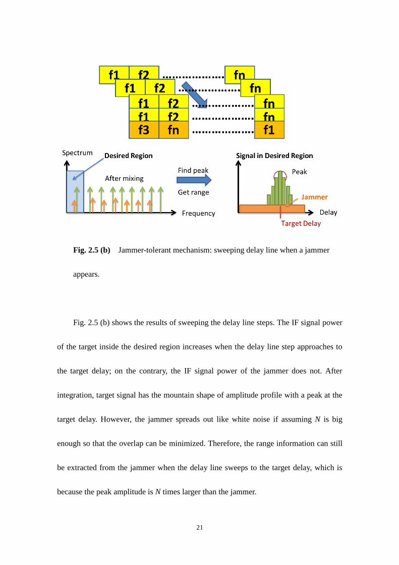
Fig. 2.5 (b) Jammer-tolerant mechanism: sweeping delay line when a jammer
appears.
Fig. 2.5 (b) shows the results of sweeping the delay line steps. The IF signal power
of the target inside the desired region increases when the delay line step approaches to
the target delay; on the contrary, the IF signal power of the jammer does not. After
integration, target signal has the mountain shape of amplitude profile with a peak at the
target delay. However, the jammer spreads out like white noise if assuming N is big
enough so that the overlap can be minimized. Therefore, the range information can still
be extracted from the jammer when the delay line sweeps to the target delay, which is
because the peak amplitude is N times larger than the jammer.
Page 36
22
2.2 Code-Division Frequency Hopping Radar System
In order to design a new system, the first step is to define the system parameters or
the specs. The key spec is the bandwidth because the resolution can be calculated by:
𝑑𝑅 =𝑐
2 ∙ 𝐵𝑊 , 𝑑𝑅: 𝑟𝑒𝑠𝑜𝑙𝑢𝑡𝑖𝑜𝑛, 𝑐: 𝑙𝑖𝑔ℎ𝑡 𝑠𝑝𝑒𝑒𝑑. (2.1)
First, choosing 500MHz as the FM bandwidth has the resolution equal to 30cm.
Second, setting the number of frequency steps to 25 has 10^25
different frequency codes ,
which is a very big number of the combination. Third, choosing the length of frequency
code sequence as 1.25us, which corresponds to 188m unambiguous range, is long
enough for the mid-range automotive radar. The unambiguous range relates to the pulse
repetition time PRT by:
𝑅𝑚𝑎𝑥 = 𝑃𝑅𝑇 ∙ 𝑐 /2, 𝑃𝑅𝑇: 𝑝𝑢𝑙𝑠𝑒 𝑟𝑒𝑝𝑒𝑡𝑖𝑡𝑖𝑜𝑛 𝑡𝑖𝑚𝑒. (2.2)
Because the frequency code sequences repeat every PRT seconds, the maximum
delay line steps of the system is PRT so as the maximum detection rage. When the target
locates farer than this range, it generates another tone every PRT second.
Page 37
23
Fig. 2.6 Simulation of the frequency hopping system with N = 25.
Fig. 2.6 shows the simulation results of the frequency hopping system with 25
frequency steps. The frequency hops with time and there are 25 non-overlapping
frequency steps, which form a pulse used for the radar detection. These 25 frequency
steps equally occupy the total FM bandwidth of 500MHz from 24GHz, so each has
20MHz sub-channel bandwidth. The frequency code jumps back to f1 every 25 steps so
that the target cannot be identified if the traveling time of the radio wave is larger than a
pulse PRT. A segment of the frequency hopping waveform is shown in Fig. 2.7. It is a
unique waveform for each different code sequence.
Page 38
24
Fig. 2.7 A segment of the frequency hopping waveform.
Fig. 2.8 shows the simulation spectrum of the code-division FH signal shown in
Fig. 2.6. The FFT operation applies to a frequency hopping pulse containing the entire
code sequence of 25 frequency steps. The frequency domain signal is similar to a
500MHz OFDM signal because both of them contain 25 frequencies within 500MHz
bandwidth. When zooming into the in-band spectrum of the frequency hopping signal
shown in Fig. 2.8 (a), the sub-channel of one frequency step can roughly be found out
and there are 25 of them shown in Fig. 2.8 (b).
Page 39
25
Fig. 2.8 (a) Simulation spectrum of the code-division FH signal: whole view.
Fig. 2.8 (b) Simulation spectrum of the code-division FH signal: enlarged view.
Page 40
26
Fig. 2.9 Mixing signals of two FH signals with the same code.
When two frequency hopping signals with same code mix together shown in Fig.
2.9 as follows:
𝐼𝐹 = 𝑅𝐹_𝑑𝑒𝑙𝑎𝑦 ∙ 𝑅𝑋_𝑟𝑥. (2.3)
If both frequency code sequences do not align to each other, which means there are
different frequencies to mix down, the IF would have the sinusoid signals with different
frequencies. Fig. 2.10 shows the simulated IF waveform of the mixing signal from
RF_delay and RX_rx after the mixer. Fig. 2.10 (a) shows the situation that two
code-division frequency hopping signals do not align to each other. The waveform of
the IF mixing signal has the average value of zero, which means the DC value is also
zero. Fig. 2.10 (b) shows the situation that two code-division frequency hopping signals
align to each other. There is an average value and this value is not zero.
Page 41
27
Fig. 2.10 (a) Simulated IF waveform of the mixing signal: two code-division
FH signals do not align to each other.
Fig. 2.10 (b) Simulated IF waveform of the mixing signal: two code-division
FH signals align to each other.
Page 42
28
Fig. 2.11 examines the simulation results of the mixing IF signal from two
code-division frequency hopping sequences shown in Fig. 2.9 in frequency domain. Fig.
2.11 (a) shows the case that two codes do not align to each other. The mixing of
different frequency codes produces the IF frequencies spreading over the available FM
bandwidth. If two frequency hopping sequences align to each other shown in Fig. 2.11
(b), there is a peak at DC. These two frequency domain results are in line with the time
domain results shown in Fig. 2.10.
Fig. 2.11 (a) Simulated IF spectrum of the mixing signal: two code-division FH
signals do not align to each other.
Page 43
29
Fig. 2.11 (b) Simulated IF spectrum of the mixing signal: two code-division FH
signals align to each other.
When the mixing signals pass through the LPF shown in Fig. 2.12, this is actually
a correlator output result as follows:
𝐵𝐵(𝜏) = ∑ ( 𝑅𝐹𝑑𝑒𝑙𝑎𝑦(𝑡 − 𝜏)𝜏𝑡=0 ∙ 𝑅𝐹_𝑟𝑥(𝑡)). (2.4)
When sweeping the delay line steps, there is a peak at target delay in the correlation plot
shown in Fig. 2.13. The target range can be calculated from this delay.
Page 44
30
Fig. 2.12 Mixing signals pass through the LPF.
For example, in Fig. 2.13, the correlation peak locates at 100ns and the corresponding
range of this delay is 15m.
Fig. 2.13 Simulated correlation plot of the code-division FH signals.
Page 45
31
Fig. 2.14 shows the resulting waveform when the code-division frequency
hopping radar receives target and jammers all together. There are 23 jammers generated
by a code generator with pseudo-random permutation of N. The receiving signals
combine the target with all of 23 jammers so that it is impossible to distinguish the
target signal and jamming interference from the waveform. However, the target can still
be extracted from this noise-like waveform after the correlation operation shown in Fig.
2.15. The jammers spread over the entire spectrum, which only raises the noise floor but
does not affect the peak detection of the code-division frequency hopping radar.
Fig. 2.14 Receiving waveform of the target with 23 jammers.
Page 46
32
Fig. 2.15 Simulated correlation plot of the target with 23 jammers.
Is there any possible situation that it may generate the ghost to ruin the detection of
the radar if N is not big enough in the pseudo-random permutation codes? Yes, if the N
is not big enough, there might be certain case that the frequency codes from different
users overlap in a certain period with certain amount of power. Fig. 2.16 shows a
manipulated case that there are 24 users with one as target and 23 as jammers among
them. When receiving all of them, the first and last frequency codes, in certain time
Page 47
33
delay, coincide in this manipulated case. In this case, a ghost happens shown in Fig.
2.17. There is still a peak in the correlation plot, but another bigger peak shows up as
ghost that is due to the jammers. Although the probability of this case happening is low,
it somehow will happen because of the randomness. Furthermore, it makes the radar
have the wrong detection and affects the safety. Therefore, a well-defined sequence is
needed to quantify the interference-tolerant performance.
Fig. 2.16 A manipulated case that will generate a ghost.
Page 48
34
Fig. 2.17 Simulated correlation plot of the manipulated case in Fig. 2.16.
Page 49
35
2.3 One-Coincidence Frequency Hopping Code
FH is a spread-spectrum (SS) technique that has been used in Bluetooth for
multi-user multiplexing. Every user follows a sequence of frequency to hop with time.
When two users occupy the same frequency channel concurrently, the coincidence or a
hit happens and it results in mutual interference. One-coincidence sequence has the
property that the maximum number of hits between any pair of sequences belonging to
the set is one [16].
2.3.1 Frequency Hopping Signal
Frequency hopping signal has the following properties shown in Fig. 2.18. The
signal length is T seconds constructed by N frequency steps with total bandwidth B. All
the frequencies are non-repeating and each frequency appears exactly once within T
seconds with sub-channel bandwidth as B/N. The frequency of kth time slot, fk, is
frequency modulated with respect to the carrier frequency f0 by:
𝑓𝑘 = 𝑓0 + 𝑦𝑖(𝑘) ∙ (𝐵/𝑁), 𝑘 = 0 ,1 , … , 𝑁 − 1. (2.5)
where, yi(k) is the placement operator which are sequence of integers called FH code.
Page 50
36
Fig. 2.18 Frequency Hopping Signal.
Choosing yi(k) as the pseudo-random permutation of N is an intuitive solution, but it
cannot have consistent performance when N is not big enough. Therefore, a
well-defined sequence is needed to quantify the interference immunity performance.
2.3.2 Hamming Correlation
The mutual interference happens when two users occupy the same frequency
channel concurrently. For a multi-user frequency hopping system, a coincidence or a hit
is when two users occupy the same sub-frequency channel. A one-coincidence sequence
is defined as the maximum number of hits between any pair of sequences belonging to
the set is one. If a code-division frequency hopping system has 25 steps, there is only
one hit from 25 sub-frequencies.
Page 51
37
The most common radar receiver is a matched filter or correlator, correlating the
reference signal with the receiving signal. The receiving signal is the delayed version of
the reference signal reflected from the target. The target can be identified through the
peak position of the auto-correlation function, corresponding to the traveling time of the
EM wave. On the other hand, the mutual interference between different users can be
quantified by cross-correlation function. The interference immunity performance of FH
code can be evaluated by periodic Hamming correlation function HXY (·), defined as
follows:
𝐻𝑋𝑌(𝜏) = ∑ ℎ(𝑋𝑖, 𝑌𝑖+𝜏)𝑁−1𝑖=0 , 0 ≤ 𝜏 ≤ 𝑁 − 1. (2.6)
𝑤ℎ𝑒𝑟𝑒 ℎ(𝑋𝑖, 𝑌𝑖+𝜏) = { 0, 𝑋𝑖 ≠ 𝑌𝑖+𝜏
1, 𝑋𝑖 = 𝑌𝑖+𝜏
The above equation defines the auto-correlation function Hrr(τ) when r = s, and
cross-correlation function Hrs(τ) when r ≠ s. From this equation, the results have a one
when two codes coincidence at certain time. If there is no coincidence, the results have
a zero. The final result is the summation of those ones and zeros for the entire sequence
of codes. The maximum non-trivial correlation value is defined as:
Page 52
38
𝐻𝑎𝑚 = 𝑚𝑎𝑥{ 𝐻𝑟𝑟 , 𝜏 = 1, … , 𝑁 − 1 } (2.7)
and
𝐻𝑐𝑚 = 𝑚𝑎𝑥{ 𝐻𝑟𝑠, 𝑟 ≠ 𝑠 , 𝜏 = 0, 1 , … , 𝑁 − 1 } (2.8)
The Ham is for auto-correlation, and it is zero ideally besides the peak. The maxima
among those non-zero values quantifies the performance of the sequence. The Hcm is for
cross-correlation, and it is one ideally in a one-coincidence sequence. Therefore, for a
FH code set S, the optimal Hamming correlation pair of S is (Ham, Hcm) = (0, 1). That is,
one-coincidence FH sequence.
2.3.3 Extended Hyperbolic Congruential Code
One of the popular methods to construct a FH code set is to use a congruential
equation. EHC code is a one-coincidence sequence with optimal Hamming correlation
property (Ham,Hcm) = (0, 1) [17]. Its placement operator, yi(k), is defined as:
𝑦𝑖(𝑘) ≡ { ( 𝑖 ∙ 𝑘 )−1 𝑚𝑜𝑑(𝑝), 𝑘 = 1, 2, … , 𝑝 − 1;
0, 𝑘 = 0. (2.9)
where p is a prime number greater than two, k is the time slot, and i is the user
identification number from {1, 2, · · · , p − 1}. By choosing N = p, an EHC code set
Page 53
39
contains N – 1 different codes for N − 1 users. Each EHC code has N different
frequencies occupying N continuous time slots, and its auto-correlation peak is Hxx = N
with Ham = 0. This is due to choosing p as a prime number that sets a finite field to
guarantee each element has a unique inverse in the modulus operation. This also ensures
that each user has N different frequencies for N continuous time slots, which utilizes the
full available FM bandwidth of the frequency hopping radar. Any pair of EHC codes
from the same EHC code set has cross-correlation Hxy = Hcm = 1. That is because the
first element is always a zero and there are no overlapping codes elsewhere. Therefore,
an EHC FH code system can accommodate N − 1 users concurrently.
The implementation of an EHC code system is shown in Fig. 2.19. First of all,
choosing zero as the start value of the sequence for the initial condition in this case. In
addition, generating
gi(k) ≡ i ▪ k mod (p) (2.10)
by using recursive addition to replace the multiplication operation defined as:
𝑔𝑖(𝑘 + 𝑖) ≡ 𝑔𝑖(𝑘) + 𝑖 𝑚𝑜𝑑(𝑝). (2.11)
This step reduces the computing complexity, which results in saving the computing
Page 54
40
power and time especially when the number is big. Finally, applying multiplicative
inverse mapping to gi(k) in order to get the yi(k) as:
𝑦𝑖(𝑘) ≡ (𝑔𝑖(𝑘))−1
𝑚𝑜𝑑(𝑝). (2.12)
where the multiplicative inverse is defined as:
(𝑔𝑖(𝑘))−1
∙ 𝑔𝑖(𝑘) ≡ 1 𝑚𝑜𝑑(𝑝). (2.13)
Fig. 2.19 Implementation of the EHC code.
Page 55
41
Using N = 5 for example to create an EHC code set as follows:
𝑈𝑠𝑒𝑟 (𝑖 = 1): { 0, 1, 3, 2, 4 } (2.14)
𝑈𝑠𝑒𝑟 (𝑖 = 2): { 0, 3, 4, 1, 2 }
𝑈𝑠𝑒𝑟 (𝑖 = 3): { 0, 2, 1, 4, 3 }
𝑈𝑠𝑒𝑟 (𝑖 = 4): { 0, 4, 2, 3, 1 }
which means user i = 1 (U1) has the frequency sequence {f0, f1, f3, f2, f4} to hop with
time and so on. Fig. 2.20 shows the Hamming correlation property of this EHC code set.
The x-axis is user id i, y-axis is the circular time shift τ , and z-axis is the magnitude of
Hamming correlation Hxy(τ ). If we choose user i = 4 (U4) as the reference (REF), other
users i = 1, 2, 3 (U1, U2, U3) are interference (INT). When reference signal correlates
with itself, resulting in an auto-correlation function, it has a peak of five at zero delay
and is zero elsewhere. When reference signal correlates with interference, resulting in
an cross-correlation function, it has the maximum level of one for all delays. That is,
(Ham, Hcm) = (0, 1), fulfills one-coincident FH code. When all four user signals sum
together, the total interference level becomes Hxy (τ) = (N −1) −1 = 3, τ ≠ 0. The signal
peak is Hxy(0) = N = 5. Therefore, the target signal can be extracted from the
interference in the multi-user environment.
Page 56
42
(a)
(b)
Fig. 2.20 Correlation property of an EHC code set with p = 5.
Page 57
43
Chapter 3
Implementation and Measurement
3.1 Implementation
Fig. 3.1 shows the implemented FH radar system block diagram. The FH
waveform generator captures the EHC codes and outputs the EHC FH waveform to
transmitter and delay unit. The receiving signal is correlated with the delayed version of
the reference signal for further DSP operation. The algorithm controls EHC code
generator, delay, and DSP to estimate the range and velocity of vehicles. The transmitter
(TX), receiver (RX), and waveform generator are calibrated through the tuning
digital-to-analog converters (DACs), which control the biasing of the circuit blocks, to
optimize the FH radar function.
Fig. 3.1 Radar system block diagram.
Page 58
44
3.1.1 Receiver
Fig. 3.2 shows the receiver architecture, including an input low-noise amplifier
(LNA), transconductor (Gm) stage, passive mixer, lowpass filter (LPF), and the
calibration DACs. The LNA amplifies the RF signal and the Gm stage converts this
voltage signal to current mode. The current signal flows through a passive mixer and is
filtered by the LPF.
Fig. 3.2 Receiver architecture.
Page 59
45
Fig. 3.3 shows the schematic of the LNA. This LNA is a transformer-coupled
single-stage differential common-source (CS) amplifier with neutralization capacitors.
The first transformer is used as a balun that converts the single-ended RF signal to
differential. The cross-coupled neutralization capacitors match the feedback parasitic
capacitance of the CS transistors to cancel out the feedback signals, which improves the
stability so does the maximum stable gain of the CS amplifier. The output transformer
provides the voltage gain for the following stage. The bias of the CS stage is controlled
by the calibration DAC.
Fig. 3.3 LNA schematic.
Page 60
46
Fig. 3.4 LNA layout.
Page 61
47
Fig. 3.4 shows the layout of the LNA where the transformer is constructed by
edge-coupled metals, which has balanced performance, low loss, and good coupling
factor.
Fig. 3.5 shows the schematic of the Gm stage. This Gm stage converts the voltage
signal to current signal with neutralization capacitors to improve the stability and stable
gain. The output transformer provides the current gain for the current-mode operation of
Fig. 3.5 Gm stage schematic.
Page 62
48
the following stage. Fig. 3.6 shows the schematic of the passive mixer and the lowpass
filter. This passive mixer operates in current mode to improve the linearity of the
receiver, and the output capacitor filters out the high frequency components after mixing
operation. Fig. 3.7 shows the combined layout of the both Gm stage and the mixer. The
transformer has 3:2 ratio to boost the current signal from the Gm stage and input to the
mixer.
Fig. 3.6 Schematic of mixer and LPF.
Page 63
49
Fig. 3.7 Layout of Gm stage and mixer.
Page 64
50
Fig. 3.8 shows the simulation results of the receiver. The maximum conversion
gain is 31.5dB in high-gain mode and is 27dB in low-gain mode both with the 3-dB
bandwidth around 2GHz shown in Fig. 3.8 (a). This also demonstrates the capability of
the calibration for the receiver conversion gain, which has accomplished by the DACs.
Fig. 3.8 (b) shows the noise figure (NF) of the receiver. The minimum NF is 4.2dB and
it has similar NF performance in both gain modes. Fig. 3.8 (c) shows the S11 of the
receiver. The S11 is lower than -10dB for the usable bandwidth in high-gain mode and
shifts to higher frequency in low-gain mode. Fig. 3.8 (d) shows the linearity of the
receiver. The input 1-dB compression point (P1dB) is -40dBm in high-gain mode and
goes up to -37.5dBm in low-gain mode.
Page 65
51
Fig. 3.8 (a) Receiver simulation results: conversion gain.
Fig. 3.8 (b) Receiver simulation results: noise figure.
Page 66
52
Fig. 3.8 (c) Receiver simulation results: S11.
Fig. 3.8 (d) Receiver simulation results: linearity.
Page 67
53
3.1.2 Power Amplifier
Fig. 3.9 shows the architecture of the power amplifier where pre-driver
provides the gain to drive the main PA and the main PA provides the power to drive the
load. This main PA also has the function of differential to single-ended convertor to
output the RF signal. The bias of both pre-driver and main PA is controlled by the
calibration DACs.
Fig. 3.9 Power amplifier architecture.
Page 68
54
Fig. 3.10 Pre-driver schematic.
Fig. 3.10 shows the schematic of the pre-diver. This pre-driver is a CS amplifier
with neutralization capacitor to improve both stability and stable gain. The additional
cross-coupled transistors at the load provide the negative-gm to cancel some portion of
the parasitic resistance in the load inductor, which minimizes the conductor loss of the
inductor. The strength of the negative-gm can be controlled by the bias current source,
which results in the gain change of the pre-driver. Fig. 3.11 shows the layout of this
pre-driver.
Page 69
55
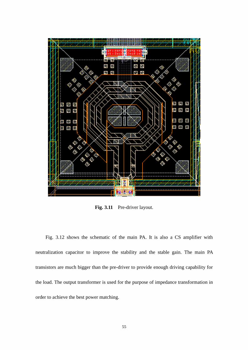
Fig. 3.11 Pre-driver layout.
Fig. 3.12 shows the schematic of the main PA. It is also a CS amplifier with
neutralization capacitor to improve the stability and the stable gain. The main PA
transistors are much bigger than the pre-driver to provide enough driving capability for
the load. The output transformer is used for the purpose of impedance transformation in
order to achieve the best power matching.
Page 70
56
Fig. 3.12 Main PA schematic.
The output capacitor is added to resonate the inductance of the output transformer
at the desired frequency. On the input side, there is also a transformer for the impedance
transformation, which provides the power matching at the source to further extend the
driving capability. The input capacitors are also added to resonate the inductance of the
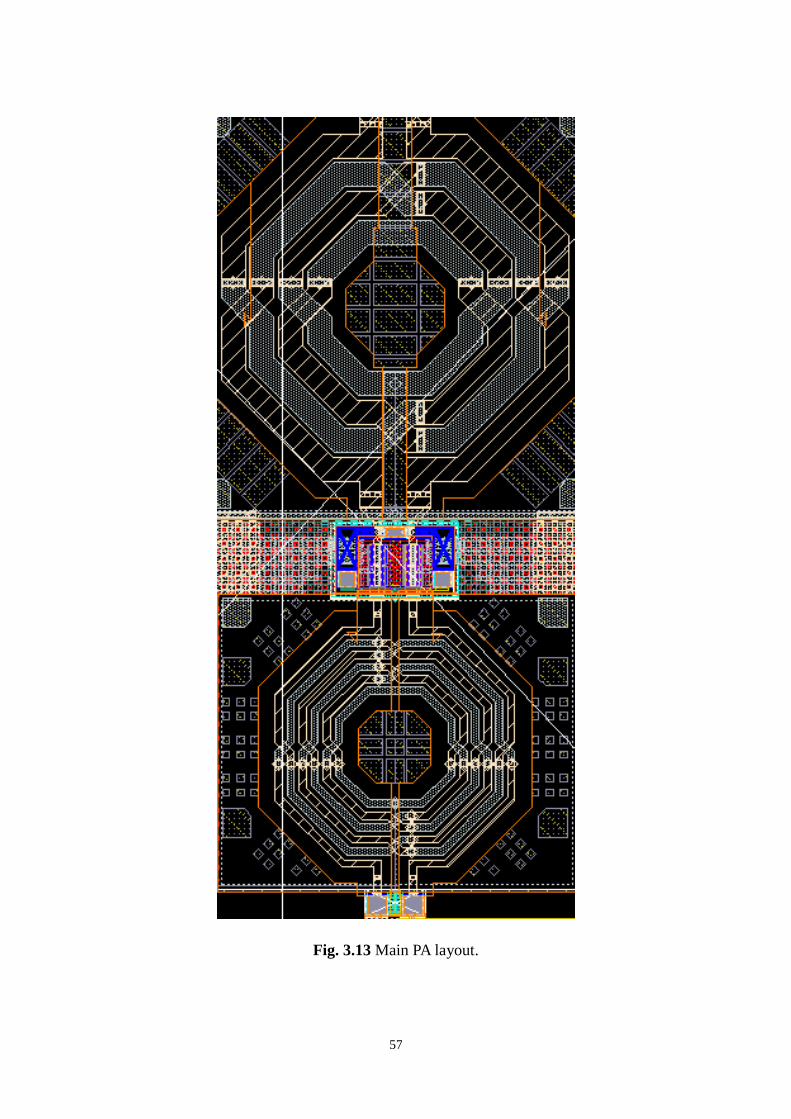
transformer at desired frequency. Fig. 3.13 shows the layout of the main PA. The metal
width of the output transformer is enlarged to accommodate the high current of the main
PA.
Page 71
57
Fig. 3.13 Main PA layout.
Page 72
58
Fig. 3.14 shows the simulation results of the power amplifier. The maximum power
gain is 10dB in high-gain mode and down to 6dB in low-gain mode shown in Fig. 3.14
(a), which demonstrates the capability of the PA gain tuning by the calibration DACs.
The 3-dB bandwidth is around 3.3GHz that is wide enough to cover the entire usable
bandwidth in both high-gain and low-gain modes. Fig. 3.14 (b) shows the linearity of
the PA with left y-axis as gain and right y-axis as output power (Pout). The output P1dB is
6.4dBm and the saturation power level is 11.5 dBm. Fig. 3.14 (c) shows the S11 of the
PA. The S11 is better than -10dB for the entire usable bandwidth.
Fig. 3.14 (a) Power amplifier simulation results: power gain.
Page 73
59
Fig. 3.14 (b) Power amplifier simulation results: linearity.
Fig. 3.14 (c) Power amplifier simulation results: S11.
Page 74
60
3.1.3 Radar Platform
Fig. 3.15 shows the implemented FH radar measurement platform. EHC code
generator produces the encoded EHC data and clock to the radar module. The data
receiver, serial-to-parallel demux, and mapping decoder are integrated on chip to drive a
FH waveform generator. The total bandwidth of the FH signal is 1GHz with 8-bit
frequency step resolution. The on-chip TX radiates at 24GHz through the horn antenna.
The RX horn antenna receives the reflected signal from the metal plate target placed 2m
away. The down-converted baseband signals are captured by oscilloscope for further
post processing on PC.
Fig. 3.16 shows the microwave radar module. This microwave module is 8cm by
4cm including the connectors, which carries the 24GHz signals, analog baseband
Fig. 3.15 Radar platform setup.
Page 75
61
signals, and high-speed digital signaling. The 24GHz signals run at top (TX), bottom
(RX), and right (LO), and each signal is connected through a dedicated high frequency
SMA connector that can work up to 26.5GHz. The baseband signals go to bottom (BB)
running with differential to minimized the coupling from other signals. The high-speed
digital signals come from top (DATA and CLK) running with lowest amplitude to
maintain the signal quality as well as minimize the interference to other signals. The test
pins monitoring the signals are build at the bottom right corner with a switch to
manually debug the DATA and CLK. The digital control interface is build with a header
(Control) to control the function of the CMOS chip. The radar IC fabricated by 65nm
CMOS includes frequency hopping generator, digital control serial interface, RF
transceiver, and calibration circuitry.
Fig. 3.16 Microwave radar module and CMOS chip.
Page 76
62
In order to get the 24GHz out from the printed circuit board (PCB), the assembly is
the major issue to deal with shown in Fig. 3.17. This PCB combines two types of
different substrates, which includes the Rogers (RO) microwave substrate on the top
and the commercial FR4 low-cost substrate for the electrical power supplies as well as
the mechanical support shown in Fig. 3.17 (a). The low loss tangent RO substrate
carries the microwave signals with low dielectric loss and good integrity. Moreover,
choosing high dielectric constant minimizes the dimension of the transmission lines
smoothing the transition between the chip and the board. The RO substrate is milled
down by the depth equal to the thickness of the CMOS chip, which minimizes the
bondwire connections as well as their parasitics.
Fig. 3.17 (a) Assembly: Rogers with FR4
Page 77
63
Fig. 3.17 (b) Assembly: milling down space.
The milling down space shown in Fig. 3.17 (b) has the ground plane to dissipate
the heat. All the 24GHz signals are carried by the coplanar waveguide (CPW) shown in
Fig. 3.17 (c) to isolate the microwave signals from other signal sources. The ground vias
of the CPW have to close to the chip as much as possible to maintain the electrical
property of the CPW at microwave frequency. The spacing of the first two ground vias
also needs to be minimized for better microwave grounding. Exposing the metal of the
CPW to the air controls the impedance well at microwave frequency. The size of both
Page 78
64
Fig. 3.17 (c) Assembly: CPW ground vias.
bonding pads on the chip and on the board are enlarged to accommodate double
bondwire on each pad to further reduce the parasitic inductance by half shown in Fig.
3.17 (d).
Fig. 3.17 (d) Assembly: double bondwire.
Page 79
65
The radar system parameters are summarized in Table 3.1. The carrier frequency is
24GHz with FM bandwidth of 1GHz corresponding to 15cm resolution. The number of
frequency step is 23 for 22 users, and the signal length is chosen so that the maximum
unambiguous range is long enough for mid-range automotive radar operation. The
measured transmit power is 4dBm and the measured NF is 9dB with the receiver gain of
22dB. These parameters are the overall system performance measured from the output
of the connectors. That is, the transmit power, conversion gain, and noise figure include
all the assembly and transition loss from the bondwires, traces, and connectors. The
bandwidth of the system also counts in the parasitics of the assembly other than the chip
itself.
Page 80
66
Parameter Value
Frequency 24GHz
Frequency Steps 23
Bandwidth 1 GHz
Frequency Steps 23
Symbol Rate 45 MHz
EHC Code Length 0.5 us
Number of Users 22
Resolution 15 cm
Maximum Unambiguous Range 75 m
Transmit Power 4 dBm
Receiver Conversion Gain 22 dB
Receiver Noise Figure 9 dB
Sideband Rejection -30 dBc@ 500 MHz
Power Consumption 143 mW
Table 3.1 Summary of FH Radar System Parameters
Page 81
67
3.2 Measurement Results
Fig. 3.18 shows the TX output spectrum of EHC FH radar at 24GHz. The
bandwidth of the FH signal is 1GHz with the sideband rejection of 30dBc at 500MHz
offset, which is the primary inherited advantage of the FH signal. There is no need for
sideband cancellation technique in direct sequence SS radars shown in Fig. 3.19 [18].
Fig. 3.18 EHC FH radar TX output spectrum at 24GHz.
Page 82
68
Fig. 3.19 DSSS Radar frequency spectrum.
In Fig. 3.19, the green curve is without sideband cancelation technique and the black
curve has it. Without sideband cancellation technique, this DSSS radar only has 13dBc
rejection due to the wideband code spreading. The sideband level goes down to 20dBc
when applying special circuit and system technique. However, in FHSS radar, it is very
easy to get 30dBc rejection due to the narrow bandwidth of frequency hopping at each
sub-band.
Page 83
69
Fig. 3.20 Measured radar SNR in multi-user environment.
Fig. 3.20 shows the signal-to-noise (SNR) versus the number of users. The SNR
decreases due to the increase of radar users and corresponding interferences.
Nevertheless, the SNR stays above 13dB (dashed line) to maintain the detection
probability Pd = 0.9 with the false alarm rate Pfa = 10−6
according to the radar cookbook,
which shows the typical detection probability versus SNR in a radar system shown in
Fig. 3.21 [19].
Page 84
70
Fig. 3.21 Typical detection probability versus SNR in a radar system.
Fig. 3.22 shows the measured range plot of the EHC FH radar in multi-user
environment. There are three different test scenarios. The first one is a single-user
environment where reference correlates with the delay version of itself, which expresses
an auto-correlation function. The red curve in Fig. 3.22 (a) is an auto-correlation
function with a peak at 2m with average -32dB noise level normalized to the signal in a
single-user environment. Obviously, the signal can be detected correctly in a single user
scenario. The maximum unambiguous range of the radar is 75m due to the 0.5us code
length.
Page 85
71
Second is that the radar receives both target and interference together. In a 2-user
environment as the cyan curve shown in Fig. 3.22 (a), the average noise level goes up to
-25dB due to the interference introduced by the second user. The peak still appears at
2m with the average noise level of -14dB, which corresponds to the sum of all
interference from other 21 users. The blue curve in Fig. 3.22 (a) shows the reference
correlates with the sum of all 22 users, including the target. In fact, the overall average
noise level is actually the sum of the auto-correlation function and the cross-correlation
function.
In order to further verify the system, the last scenario shown in Fig. 3.22 (b) is that
Fig. 3.22 (a) Measured range plot: auto-correlation in single-user (red) environment and
correlation in 2-user (cyan) and 22-user (blue) environment.
Page 86
72
the radar receives only the interference from other users but no signals from the target.
In this scenario, the reference signal correlates with other users that have different EHC
codes, i.e., the cross-correlation function. The average interference level is around
-26dB in a 2-user environment and -14dB in a 22-user environment, which matches to
the results shown in Fig. 3.22 (a). Therefore, the result that the interference level is
well-managed in EHC FH radar system has been verified. From these measurement
results, this code-division FH radar can detect targets correctly in a multi-users scenario
up to 22 of them. These results prove that EHC FH code has the needed interference
immunity property for intended multi-user radar system.
Fig. 3.22 (b) Measured range plot: cross-correlation in 2-user (cyan) and 22-user (blue)
environment.
Page 87
73
Chapter 4
Conclusions
In this dissertation, the potential radar interference issue for future multi-vehicle
autonomous driving system has been addressed. An extended hyperbolic congruential
(EHC) code as the one-coincidence frequency hopping (FH) code has been
implemented in the CMOS radar prototype at 24GHz and its excellent performance has
been validated. The interference level is well-managed in this EHC FH radar system
with optimal Hamming correlation property.
An interference-tolerant multi-user radar system, based on the EHC FH code in a
multi-vehicle environment for autonomous driving applications, has been realized. Up
to 22 vehicles can co-operate at the same time/area with 1GHz bandwidth and with
minimum 15cm range resolution.
Page 88
74
References
[1] “Look, No Hands,” The Economist, Sep. 12, 2012.
http://www.economist.com/node/21560989
[2] Josie Garthwaite “Sharing the Road With Driverless Cars,” Beacon, May 12,
2014.
https://www.beaconreader.com/climate-confidential/sharing-the-road-with-drive
rless-cars
[3] M. Steinhauer, H. O. Ruob, H. Irion and W. Menzel, “Millimeter-Wave-Radar
Sensor Based on a Transceiver Array for Automotive Applications,” IEEE Trans.
Microw. Theory Techn., vol. 56, no. 2, pp. 261-269, Feb. 2008.
[4] S. T. Nicolson et al., "A Low-Voltage SiGe BiCMOS 77-GHz Automotive
Radar Chipset," IEEE Trans. Microw. Theory Techn., vol. 56, no. 5, pp.
1092-1104, May 2008.
[5] R. Feger, C. Wagner, S. Schuster, S. Scheiblhofer, H. Jager and A. Stelzer, "A
77-GHz FMCW MIMO Radar Based on an SiGe Single-Chip Transceiver,"
IEEE Trans. Microw. Theory Techn., vol. 57, no. 5, pp. 1020-1035, May 2009.
[6] N. Pohl, T. Jaeschke and K. Aufinger, "An Ultra-Wideband 80 GHz FMCW
Radar System Using a SiGe Bipolar Transceiver Chip Stabilized by a
Fractional-N PLL Synthesizer," IEEE Trans. Microw. Theory Techn., vol. 60, no.
3, pp. 757-765, March 2012.
[7] S. Trotta et al., "An RCP Packaged Transceiver Chipset for Automotive LRR
and SRR Systems in SiGe BiCMOS Technology," IEEE Trans. Microw. Theory
Techn., vol. 60, no. 3, pp. 778-794, March 2012.
[8] J. Hasch, E. Topak, R. Schnabel, T. Zwick, R. Weigel and C. Waldschmidt,
"Millimeter-Wave Technology for Automotive Radar Sensors in the 77 GHz
Frequency Band," IEEE Trans. Microw. Theory Techn., vol. 60, no. 3, pp.
845-860, March 2012.
[9] J. Yu et al., "An X-Band Radar Transceiver MMIC with Bandwidth Reduction
in 0.13 µm SiGe Technology," IEEE J. Solid-State Circuits, vol. 49, no. 9, pp.
Page 89
75
1905-1915, Sept. 2014.
[10] B. H. Ku et al., "A 77–81-GHz 16-Element Phased-Array Receiver With ±50∘
Beam Scanning for Advanced Automotive Radars," IEEE Trans. Microw.
Theory Techn., vol. 62, no. 11, pp. 2823-2832, Nov. 2014.
[11] T. Jaeschke, C. Bredendiek, S. Küppers and N. Pohl, "High-Precision D-Band
FMCW-Radar Sensor Based on a Wideband SiGe-Transceiver MMIC," IEEE
Trans. Microw. Theory Techn., vol. 62, no. 12, pp. 3582-3597, Dec. 2014.
[12] T. Mitomo, N. Ono, H. Hoshino, Y. Yoshihara, O. Watanabe and I. Seto, "A 77
GHz 90 nm CMOS Transceiver for FMCW Radar Applications," IEEE J.
Solid-State Circuits, vol. 45, no. 4, pp. 928-937, April 2010.
[13] J. Lee, Y. A. Li, M. H. Hung and S. J. Huang, "A Fully-Integrated 77-GHz
FMCW Radar Transceiver in 65-nm CMOS Technology," IEEE J. Solid-State
Circuits, vol. 45, no. 12, pp. 2746-2756, Dec. 2010.
[14] C. Cui, S. K. Kim, R. Song, J. H. Song, S. Nam and B. S. Kim, "A 77-GHz
FMCW Radar System Using On-Chip Waveguide Feeders in 65-nm CMOS,"
IEEE Trans. Microw. Theory Techn., vol. 63, no. 11, pp. 3736-3746, Nov. 2015.
[15] T.-N. Luo et al., “A 77-GHz CMOS FMCW Frequency Synthesizer with
Reconfigurable Chirps,” IEEE Trans. Microw. Theory Techn., vol. 61, no. 7, pp.
2641-2647, July 2013.
[16] L. Bin, “One-Coincidence Sequences with Specified Distance Between Adjacent
Symbols for Frequency-Hopping Multiple Access,” IEEE Trans. Commun., vol.
45, no. 4, pp. 408-410, Apr 1997.
[17] L. Wronski et al., “Extended Hyperbolic Congruential Frequency Hop Code:
Generation and Bounds for Cross- and Auto-Ambiguity Function,” IEEE Trans.
Commun., vol. 44, no. 3, pp. 301-305, Mar 1996.
[18] V. Giannini et al., “A 79 GHz Phase-Modulated 4 GHz-BW CW Radar
Transmitter in 28 nm CMOS,” IEEE J. Solid-State Circuits, vol. 49, no. 12, pp.
2925-2937, Dec 2014.
Page 90
76
[19] Robert M. O’Donnell, courtesy of IEEE New Hampshire Section Guest Lecturer,
Jan 2011.